Minimal $n$-Noids in hyperbolic and anti-de Sitter 3-space

Abstract.

We construct minimal surfaces in hyperbolic and anti-de Sitter 3-space with the topology of a $n$-punctured sphere by loop group factorization methods. The end behavior of the surfaces is based on the asymptotics of Delaunay-type surfaces, i.e., rotational symmetric minimal cylinders. The minimal surfaces in $\mathrm{H}^{3}$ extend to Willmore surfaces in the conformal 3-sphere $S^{3}=\mathrm{H}^{3}\cup\mathrm{S}^{2}\cup\mathrm{H}^{3}$.

Introduction

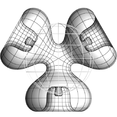
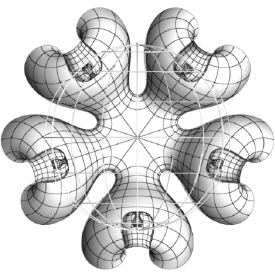
Figure 1. Cutaway views of equilateral minimal noids in $\mathrm{H}^{3}\cup\mathrm{S}^{2}\cup\mathrm{H}^{3}$ with end counts and cyclic symmetry orders $3$ and $5$. In all figures, the surface is stereographically projected to $\mathbb{R}^{3}$, the wireframe designates the ideal boundary, and the lines on the surface are curvature lines.

The AdS/CFT correspondence predicts that the physics of the gravitational theory of anti-de Sitter (AdS) spacetime is equivalent to the physics of conformal field theory (CFT) on the boundary of that spacetime [23]. A particularly important instance is the computation of the Wilson loop expectation value, which by work of Maldacena is given by the (regularized) area of a spacelike minimal surface in AdS spacetime with the loop as boundary [11, 1, 2, 28]. The aim of this paper is to provide new examples of minimal surfaces in anti-de Sitter spaces of non-trivial topological type and with several boundary components.

It is well known that the equations for minimal surfaces in anti-de Sitter space are related to Hitchin self-duality equations [19, 2]. In particular, minimal surfaces in $\mathrm{AdS}_{3}$ are given by solutions corresponding to points in the Hitchin component for rank 2, and minimal surfaces in a totally geodesic $\mathrm{H}^{3}\subset\text{AdS}_{4}$ are given by rank 2 solutions of the self-duality equations with nilpotent Higgs field. As those, they fall into the class of integrable PDEs, and there are powerful tools for computing large classes of examples [29, 24, 9]. On the other hand, it is hard to construct surfaces with non-trivial finitely generated topology which are complete, i.e., the surface can be continued to the boundary at infinity of the anti-de Sitter space, and the intersection is a finite number of topological circles. It is worth remarking that surfaces given by global solutions of the self-duality equations are not of that much interest in the AdS/CFT correspondence as the extrinsic monodromy is always non-trivial and the intersection with the boundary at infinity gets very complicated. By finite gap integration, cylindrical solutions have been constructed; see for example [4]. In [12] a detailed numerical study for surfaces bounded by a finite number of special curves (including circles, (super)ellipses and boundaries of spherocylinders) is carried out, and the holographic entanglement entropy and the holographic mutual information for those entangling curves have been numerically computed.

For the construction of meaningful examples via loop group factorization methods, two main problems need to be solved: The first is the proof of existence of potentials depending on a loop parameter on a surface with non-trivial monodromy which satisfy a certain reality condition (see remark 1.8). This reality condition is given explicitly only by solving ODEs along non-trivial curves. We solve this problem for a large class of examples. The second problem is concerned with the construction of the minimal surfaces from potentials satisfying the reality conditions: this problem is based on the fact that the generalized Iwasawa factorization is not global, i.e., there exit loops which do not admit an Iwasawa factorization (remark 1.7). It is hard to determine the curves on the surface along which the factorization breaks down, and to characterize the behavior of the minimal surface along those curves in general. On the other hand, under a mild assumption on the degeneracy of the Iwasawa decomposition, the minimal surface intersects the boundary at infinity transversally; see for example [16, section 5] for technical details and figures 2(a) and 1 for visualizations. It is this failure of the global Iwasawa decomposition which allows us to produce minimal surfaces in anti-de Sitter spaces with non-trivial (finitely generated) topology and predicted topological intersections with the boundary at infinity, at least numerically. We plan to investigate the remaining theoretical questions concerning the intersections at infinity in forthcoming work.

The structure of the paper is as follows: In section 1 we briefly describe a unified loop group approach for constant mean curvature surfaces in the symmetric spaces $\mathrm{S}^{3}$, $\mathrm{AdS}_{3}$, $\mathrm{H}^{3}\cup\mathrm{H}^{3}$ and $\mathrm{dS}_{3}$, including the case of minimal surfaces. In section 2 we first recall the conformal surface geometry in the lightcone model, with special emphasis on minimal surfaces in hyperbolic space. We discuss some simple examples of minimal surfaces in $\mathrm{H}^{3}$: the hyperbolic disk as the counterpart of the round sphere, and minimal Delaunay cylinders. We then define $n$-noids and open $n$-noids, motivated by the behavior of Delaunay cylinders at their ends. We prove the existence of open $n$-noids, and conjecture that those surfaces actually give rise to $n$-noids in the strict sense. In section 3, we explain how to modify the techniques of section 2 in order to obtain minimal surfaces in $\mathrm{AdS}_{3}$. In section 4 we study surfaces with three ends more explicitly via the generalized Weierstrass representation (GWR); these investigations have enabled us to perform computer experiments. Among others we construct a family of equilateral trinoids in $\mathrm{H}^{3}$ with mean curvature $|H|<1$. The paper is supplemented by figures visualizing global properties of minimal surfaces in $\mathrm{H}^{3}$, $\mathrm{dS}_{3}$ and $\mathrm{AdS}_{3}$.

1   The loop group method for CMC surfaces in symmetric spaces

1.1   Unitary frames

To construct constant mean curvature (CMC) surfaces in the symmetric spaces $\mathrm{S}^{3}$, $\mathrm{AdS}_{3}$, $\mathrm{H}^{3}\cup\mathrm{H}^{3}$ and $\mathrm{dS}_{3}$ we use the following matrix models in $\mathrm{SL}_{2}(\mathbb{C})$:

(1.1) $$\begin{array}[]{l|l|l}\text{space}&\text{matrix model}&\hphantom{-}\langle x,\,y\rangle\\ \hline\cr\mathrm{S}^{3}&\mathrm{SU}_{2}&\hphantom{-}\tfrac{1}{2}\operatorname{tr}x\hat{y}\\ \mathrm{AdS}_{3}&\mathrm{SU}_{11}&-\tfrac{1}{2}\operatorname{tr}x\hat{y}\\ \mathrm{H}^{3}\cup\mathrm{H}^{3}&\{X\in\mathrm{SL}_{2}(\mathbb{C})\mid{{\overline{X}}^{\mathrm{t}}}=X\}&-\tfrac{1}{2}\operatorname{tr}x\hat{y}\\ \mathrm{dS}_{3}&\{X\in\mathrm{SL}_{2}(\mathbb{C})\mid{{\overline{X}}^{\mathrm{t}}}=e_{0}Xe_{0}^{-1}\}&\hphantom{-}\tfrac{1}{2}\operatorname{tr}x\hat{y}\end{array}$$

where $e_{0}=\operatorname{diag}(\mathbbm{i},\,-\mathbbm{i})$. The third column of the table specifies the inner product on $\mathrm{M}_{2\times 2}(\mathbb{C})$ extending the metric on the symmetric space, with sign chosen so that the signature of the tangent space is $(\pm,\,+\,+)$. Here $\hat{y}=\bigl{[}\begin{smallmatrix}d&-b\\ -c&a\end{smallmatrix}\bigr{]}$ for $y=\bigl{[}\begin{smallmatrix}a&b\\ c&d\end{smallmatrix}\bigr{]}$.

To use integrable systems methods we introduce the loop group $\Lambda\mathrm{SL}_{2}(\mathbb{C})$ of real analytic maps $\mathrm{S}^{1}\to\mathrm{SL}_{2}(\mathbb{C})$, and the subgroup $\Lambda_{+}\mathrm{SL}_{2}(\mathbb{C})$ of loops which extend holomorphically to the interior of the unit disk. The four involutions of $\Lambda\mathrm{SL}_{2}(\mathbb{C})$

(1.2) $$\begin{array}[]{l|l}\mathrm{S}^{3}&X^{\ast}(\lambda)={{\overline{X(1/\overline{\lambda})}}^{\mathrm{t}}}^{-1}\\ \mathrm{AdS}_{3}&X^{\ast}(\lambda)=e_{0}{{\overline{X(1/\overline{\lambda})}}^{\mathrm{t}}}^{-1}e_{0}^{-1}\\ \mathrm{H}^{3}&X^{\ast}(\lambda)={{\overline{X(-1/\overline{\lambda})}}^{\mathrm{t}}}^{-1}\\ \mathrm{dS}_{3}&X^{\ast}(\lambda)=e_{0}{{\overline{X(-1/\overline{\lambda})}}^{\mathrm{t}}}^{-1}e_{0}^{-1}\end{array}$$

determine four real forms $\{X\in\Lambda\mathrm{SL}_{2}(\mathbb{C})\mid X^{\ast}=X\}\subset\Lambda\mathrm{SL}_{2}(\mathbb{C})$. By an abuse of terminology, we call elements of such a subgroup unitary, or emphasizing the involution e.g. $\mathrm{H}^{3}$-unitary. We will also denote by ^∗ the corresponding involutions of the Lie algebra $\Lambda\mathrm{sl}_{2}(\mathbb{C})$.

Given a choice of one of the real forms induced by (1.2), a unitary connection is a $\Lambda\mathrm{sl}_{2}(\mathbb{C})$-valued $1$-form $\eta$ on a Riemann surface $\Sigma$ with the following properties:

• $\eta$ is flat for all $\lambda$.

• $\eta=\eta^{\ast}$.

• $\eta$ has a simple pole at $\lambda=0$, $\eta_{-1}:=\operatorname*{res}_{\lambda=0}\eta$ has no $(0,\,1)$ part, $\det\eta_{-1}=0$, and $\langle\eta_{-1},\,\eta_{-1}^{\ast}\rangle\neq 0$.

A unitary frame $F$ is a unitary solution to the ODE $\mathrm{d}F=F\eta$.

The evaluation formula maps a unitary frame to the symmetric space:

(1.3) $$f=\left.F\right|_{\lambda_{0}}\left.F^{-1}\right|_{\lambda_{1}}$$

where $\lambda_{0},\,\lambda_{1}\in\mathbb{C}^{\ast}$ are the evaluation points as follows:

(1.4) $$\begin{array}[]{l|l|l}\text{space}&\text{evaluation points}&\text{mean curvature $H$}\\ \hline\cr\mathrm{S}^{3}\text{ and }\mathrm{AdS}_{3}&\lambda_{0},\,\lambda_{1}\in\mathrm{S}^{1}\text{ distinct}&\frac{\mathbbm{i}(\lambda_{1}+\lambda_{0})}{\lambda_{1}-\lambda_{0}}\\ \mathrm{H}^{3}\text{ and }\mathrm{dS}_{3}&\lambda_{0},\,\lambda_{1}\in\mathbb{C}^{\ast}\text{ with }\lambda_{0}\overline{\lambda_{1}}=-1&\frac{\lambda_{1}+\lambda_{0}}{\lambda_{1}-\lambda_{0}}\end{array}$$

The third column of the table lists the mean curvature $H$ of the induced immersion $f$ up to sign, derived in theorem 1.1. Note that $H$ satisfies $|H|<1$ for the symmetric spaces $\mathrm{H}^{3}$ and $\mathrm{dS}_{3}$. Formula (1.3) was first derived in [5] for CMC surfaces in $\mathrm{H}^{3}$ and $\mathrm{S}^{3}.$

Theorem 1.1.

Let $\eta$ be a unitary connection on a Riemann surface $\Sigma$ with respect to one of the four real forms (1.2). Let $F$ be a unitary frame satisfying $\mathrm{d}F=F\eta$. Then the evaluation formula (1.3) evaluated at evaluation points (1.4) yields a spacelike conformal CMC immersion $f$ into the corresponding symmetric space with metric

(1.5) $$v^{2}\mathrm{d}z\otimes\mathrm{d}\bar{z},\quad v^{2}=2(\lambda_{0}^{-1}-\lambda_{1}^{-1})(\lambda_{0}-\lambda_{1})\langle\alpha,\,\alpha^{\ast}\rangle$$

and constant mean curvature as in (1.4).

Remark 1.2.

The unitary connection $\eta$ is usually referred to as the associated family of flat connections of the surface $f$.

Proof.

We prove the theorem for $\mathrm{AdS}_{3}$; the proof for the other symmetric spaces is similar with sign changes. The unitary connection decomposes as

(1.6) $$\eta=(\alpha\lambda^{-1}+\beta)\mathrm{d}z+(\beta^{\ast}+\alpha^{\ast}\lambda)\mathrm{d}\bar{z}.$$

The flatness of $\eta$ is equivalent to

(1.7) $$[\alpha,\,\beta^{\ast}]=\alpha_{\bar{z}},\quad[\alpha,\,\alpha^{\ast}]+[\beta,\,\beta^{\ast}]=\beta_{\bar{z}}-{(\beta^{\ast})}_{z},\quad[\beta,\,\alpha^{\ast}]={(\alpha^{\ast})}_{z}.$$

Let $F_{0}=\left.F\right|_{\lambda_{0}}$ and $F_{1}=\left.F\right|_{\lambda_{1}}$. To compute the metric

(1.8) $$f_{z}=(\lambda_{0}^{-1}-\lambda_{1}^{-1})F_{0}\alpha F_{1}^{-1},\quad f_{\bar{z}}=(\lambda_{0}-\lambda_{1})F_{0}\alpha^{\ast}F_{1}^{-1}.$$

Since $\langle f_{z},\,f_{z}\rangle=\langle f_{\bar{z}},\,f_{\bar{z}}\rangle=0$ the metric is $v^{2}\mathrm{d}z\otimes\mathrm{d}\bar{z}$ with

(1.9) $$v^{2}=2\langle f_{z},\,f_{\bar{z}}\rangle=2(\lambda_{0}^{-1}-\lambda_{1}^{-1})(\lambda_{0}-\lambda_{1})\langle\alpha,\,\alpha^{\ast}\rangle.$$

Since $\lambda_{0}\neq\lambda_{1}$ and $\langle\alpha,\,\alpha^{\ast}\rangle\neq 0$, the metric is nonzero, so the evaluation formula induces a conformal immersion.

The normal is $N=F_{0}\gamma F_{1}^{-1}$ where

(1.10) $$\gamma=-\frac{\mathbbm{i}}{2}\frac{[\alpha,\,\alpha^{\ast}]}{\langle\alpha,\,\alpha^{\ast}\rangle}.$$

Using flatness,

(1.11) $$f_{z\bar{z}}=(\lambda_{0}^{-1}-\lambda_{1}^{-1})F_{0}(\lambda_{0}\alpha^{\ast}\alpha-\lambda_{1}\alpha\alpha^{\ast})F_{1}^{-1}.$$

Using that $\langle\alpha\alpha^{\ast}+\alpha^{\ast}\alpha,\,\gamma\rangle=0$, the mean curvature of $f$ is

(1.12) $$H=2v^{-2}\langle f_{z\bar{z}},\,N\rangle=-\tfrac{1}{2}v^{2}(\lambda_{0}^{-1}-\lambda_{1}^{-1})(\lambda_{0}+\lambda_{1})\langle[\alpha,\,\alpha^{\ast}],\,\gamma\rangle=\mathbbm{i}\frac{\lambda_{1}+\lambda_{0}}{\lambda_{1}-\lambda_{0}}.\qed$$

Remark 1.3.

With other choices of evaluation formulas and evaluation points, CMC surfaces can also be constructed from unitary connections in the symmetric spaces related by the Lawson correspondence:

(1.13) corresponding to $$\mathrm{S}^{3} :\ \quad\text{$\mathrm{H}^{3}$ ($|H|>1$) and $\mathbb{R}^{3}$}$$

(1.14) corresponding to $$\mathrm{AdS}_{3} :\quad\text{$\mathrm{dS}_{3}$ ($|H|>1$) and $\mathbb{R}^{2,1}$}.$$

Remark 1.4.

In the case the Hopf differential is $\mathrm{d}z^{2}$, after a coordinate change the flatness of the unitary connection is Gauss equation on the metric $v^{2}=e^{2u}$:

(1.15) $$\mathrm{S}^{3} :\ \Delta u+2\sinh 2u=0 \mathrm{H}^{3}\ (|H|<1) :\ \Delta u-2\cosh 2u=0$$

(1.16) $$\mathrm{AdS}_{3} :\ \Delta u-2\sinh 2u=0 \mathrm{dS}_{3}\ (|H|<1) :\ \Delta u+2\cosh 2u=0.$$

1.2   Holomorphic frames

To construct CMC immersions by theorem 1.1, one is required to produce a flat unitary connection. The flatness is the Gauss equation, a partial differential equation on the metric. This section introduces the generalized Weierstrass representation (GWR) [10]. In this construction, the PDE is replaced by an ordinary differential equation together with a Iwasawa loop group factorization. For a more comprehensive treatment of real forms of loop groups see [22]. The case $\mathbb{R}^{2,1}$ was considered in [7].

A GWR potential $\xi$ is a $\Lambda\mathrm{sl}_{2}(\mathbb{C})$-valued $(1,\,0)$-form on a Riemann surface $\Sigma$ satisfying the following condition: $\xi$ has a simple pole at $\lambda=0$, and $\xi_{-1}:=\operatorname*{res}_{\lambda=0}\xi$ satisfies $\det\xi_{-1}=0$ and is nowhere zero. A GWR frame $\Phi$ for $\xi$ is a holomorphic map from the domain to $\Lambda\mathrm{sl}_{2}(\mathbb{C})$ satisfying $\mathrm{d}\Phi=\Phi\xi$. Choosing a real form, an Iwasawa factorization of $\Phi$ is

(1.17) $$\Phi=FB,\quad F^{\ast}=F\text{ and }B\in\Lambda_{+}\mathrm{SL}_{2}(\mathbb{C}).$$

The Iwasawa factorization can be computed via the Birkhoff factorization as follows. When in the big cell, ${\Phi^{\ast}}^{-1}\Phi$ has a Birkhoff factorization

(1.18) $${\Phi^{\ast}}^{-1}\Phi={X_{+}^{\ast}}^{-1}X_{+},\quad X_{+}\in\Lambda_{+}\mathrm{SL}_{2}(\mathbb{C}).$$

Then the desired Iwasawa factorization of $\Phi$ is

(1.19) $$\Phi=FB,\quad F:=\Phi X_{+}^{-1},\quad B:=X_{+}$$

because $F^{\ast}=F$.

Theorem 1.5.

Let $\xi$ be a GWR potential, and $\Phi$ a corresponding GWR frame. If $\Phi$ has an Iwasawa factorization, then $F$ is a unitary frame. Hence by theorem 1.1 $F$ induces a conformal CMC immersion.

Proof.

Since $\mathrm{d}\Phi=\Phi\xi$, $\mathrm{d}F=F\eta$, and $\Phi=FB$, then

(1.20) $$\eta=\xi.(B^{-1})$$

where the dot denotes the gauge action $\xi.g:=g^{-1}\xi g+g^{-1}\mathrm{d}g$. Since $B\in\Lambda\mathrm{SL}_{2}(\mathbb{C})$ and $\xi$ has a simple pole in $\lambda$, then $\eta$ has a simple pole in $\lambda$. Since $\xi$ has no $(0,\,1)$ part, then $\eta_{-1}:=\operatorname*{res}_{\lambda=0}\eta$ has no $(0,\,1)$ part. Since $F^{\ast}=F$, then $\eta^{\ast}=\eta$, hence $\eta$ is a unitary connection. ∎

Remark 1.6.

The Hopf differential of CMC immersion induced by a GWR potential $\xi$ is of the form $c(\lambda)Q\mathrm{d}z^{2}$ where $c$ is $z$-independent and $Q$ is the leading term (coefficient of $\lambda^{-1})$ of $\det\xi$.

Remark 1.7.

In the case of the spaceform $\mathrm{S}^{3}$, the GWR frame always has an Iwasawa factorization. For the other three real forms, the GWR frame may fail to have an Iwasawa factorization, generally on some real analytic subset of the domain. On this set the surface is singular, in many cases going to the ideal boundary.

If the domain is not simply connected, $\Phi$ has monodromy and the induced CMC immersion on the universal cover does not generally close, that is, descend to an immersion of the domain. A sufficient condition for closing is the following:

Remark 1.8.

The induced CMC immersion closes if the monodromy $M$ of $\Phi$ is unitary (intrinsic closing), and at the evaluation points $M(\lambda_{0})=M(\lambda_{1})\in\{\pm 1\}$ (extrinsic closing).

2   Minimal $n$-noids in hyperbolic 3-space

We study minimal surfaces in hyperbolic 3-space $\mathrm{H}^{3}$ which intersect the boundary at infinity perpendicularly. A convenient setup from a geometric point of view is conformal surface geometry in the lightcone model of the 3-sphere.

2.1   The lightcone model for $\mathrm{H}^{3}$

The lightcone approach to conformal surface geometry is classical; for details we refer to [8, 26] and the references therein. We consider Minkowski space $V=\mathbb{R}^{4,1}$ with its standard inner product $(\cdot,\,\cdot)$ inducing the quadratic form

(2.1) $$q(x_{0},\dots,x_{4})=-x_{0}^{2}+x_{1}^{2}+\dots+x_{4}^{2}.$$

The lightcone

(2.2) $$\mathcal{L}=\{\mathbb{R}x\in PV\mid x\neq 0,\;q(x)=0\}$$

is diffeomorphic to the 3-sphere $\mathrm{S}^{3}$ via

(2.3) $$(x_{1},\dots,x_{4})\in\mathrm{S}^{3}\ \mapsto\ \mathbb{R}(1,x_{1},\dots,x_{4})\in\mathcal{L}.$$

Thus $\mathcal{L}$ inherits a conformal structure from the round metric on $\mathrm{S}^{3}$. It is well known that the group $\mathrm{SO}(4,1)$ acts on $\mathcal{L}$ by conformal transformations. In fact,

(2.4) $$\mathrm{SO}_{+}(4,1)=\{g\in\mathrm{SO}(4,1)\mid(g(e_{0}),e_{0})>0\}$$

is the group of (orientation preserving) conformal diffeomorphisms of $\mathrm{S}^{3}$ (equipped with the round conformal structure).

2.1.1   Hyperbolic 3-space

Taking the spacelike vector $v_{\infty}=e_{4}$ we obtain two copies of hyperbolic 3-space as

(2.5) $$\mathcal{L}\setminus(\mathcal{L}\cap P(e_{4}^{\perp}))=\{(x_{0},x_{1},x_{2},x_{3},-1)\mid-x_{0}^{2}+x_{1}^{2}+x_{2}^{2}+x_{3}^{2}=-1\}.$$

This space is naturally equipped with the metric of constant curvature $-1$. The subgroup $\mathrm{SO}_{+}(3,1)\subset\mathrm{SO}_{+}(4,1)$ (defined by fixing the vector $e_{4}$) realizes the isometry group of hyperbolic 3-space.

2.1.2   Surfaces in the lightcone model

We consider conformal immersions

(2.6) $$f\colon\Sigma\to\mathrm{S}^{3}$$

from a Riemann surfaces $\Sigma$ into the conformal 3-sphere. The map $f$ is equivalent (in conformal geometry) to the line bundle of light-like vectors

(2.7) $$\sigma^{\ast}\mathcal{L}\to\Sigma$$

for $\sigma=(1,f)$. The fact that $f$ is an immersion means that for any (local) lift $\tilde{\sigma}=g\sigma$ and (local) pointwise independent vector fields $X,Y$ on $\Sigma$

(2.8) $$\text{span}(\tilde{\sigma},\,X\cdot\tilde{\sigma},\,Y\cdot\tilde{\sigma})$$

is a (real) 3-dimensional bundle (where $\cdot$ denotes the derivative). Conformality of $f$ means that for a local holomorphic chart $z$ on $\Sigma$ we have

(2.9) $$(\tilde{\sigma}_{z},\tilde{\sigma}_{z})=0=(\tilde{\sigma}_{\bar{z}},\tilde{\sigma}_{\bar{z}})$$

where $g_{z}:=\frac{\partial}{\partial z}\cdot g$ and $g_{\bar{z}}:=\frac{\partial}{\partial\bar{z}}\cdot g$ for any (vector-valued) function $g$.

A fundamental object in conformal surface theory is the mean curvature sphere congruence. The mean curvature sphere is defined locally by

(2.10) $$\mathcal{S}=\text{span}(\tilde{\sigma},\,\tilde{\sigma}_{z},\,\sigma_{\bar{z}},\,\tilde{\sigma}_{z,\bar{z}}).$$

Proposition 2.1.

The surface $f$ considered as a surface in hyperbolic 3-space defined by $v_{\infty}=e_{4}$ is of constant mean curvature $H$ if and only if

(2.11) $$H=(e_{4}^{\perp},\,e_{4}^{\perp})$$

is constant, where $(e_{4}^{\perp})_{p}$ is the projection of $e_{4}$ to $\mathcal{S}_{p}$. Consequently, $f$ is minimal if and only if $e_{4}$ is contained (as a constant section) in $\mathcal{S}$.

In the following, we are interested in conformally parametrized surfaces $f\colon\Sigma\to\mathrm{S}^{3}$ into the conformal 3-sphere such that its intersection with

(2.12) $$\mathrm{H}^{3}\cup\mathrm{H}^{3}\ =\ \mathrm{S}^{3}\setminus\mathrm{S}^{2}\ =\ \mathcal{L}\setminus(\mathcal{L}\cap P(e_{4}^{\perp}))$$

is a minimal surface. In order to apply the GWR approach we need an explicit isometry

(2.13) $$\Psi\colon\mathcal{L}\setminus(\mathcal{L}\cap P(e_{4}^{\perp}))\to\{X\in\mathrm{SL}_{2}(\mathbb{C})\mid{{\overline{X}}^{\mathrm{t}}}=X\}.$$

This is provided by

(2.14) $$\Psi([x_{0},x_{1},x_{2},x_{3},x_{4}])\mapsto\frac{1}{x_{4}}\begin{bmatrix}x_{0}+x_{1}&x_{2}+ix_{3}\\ x_{2}-ix_{3}&x_{0}-x_{1}\end{bmatrix}.$$

Note that the two copies of $\Psi(\mathcal{L}\setminus(\mathcal{L}\cap P(e_{4}^{\perp})))$ are given by the sets of positive definite and negative definite symmetric $\mathrm{SL}_{2}$-matrices.

2.2   Basic examples

We first illustrate the GWR approach for some basic surfaces. Recall that for $\mathrm{H}^{3}$, the real involution on $\Lambda\mathrm{SL}_{2}(\mathbb{C})$ is given by

(2.15) $$X^{\ast}(\lambda)=e_{0}\overline{X(-1/\bar{\lambda})}^{-1}e_{0}^{-1},$$

and unitary connections are flat connections of the form

(2.16) $$d+\eta(\lambda)=d+\eta_{0}+\lambda^{-1}\eta_{-1}+\lambda\eta_{1}$$

with ${\overline{\eta_{0}}}^{\mathrm{t}}=-\eta_{0}$ and ${\overline{\eta_{-1}}}^{\mathrm{t}}=\eta_{1}$ where $\eta_{-1}$ is a nowhere vanishing $(1,0)$-form with values in the nilpotents.

2.2.1   The sphere in $\mathrm{H}^{3}$

The simplest example of a GWR potential is given by

(2.17) $$\xi(\lambda)=\begin{bmatrix}0&\lambda^{-1}\\ 0&0\end{bmatrix}dz$$

on the complex plane, with GWR frame

(2.18) $$\Phi(\lambda)=\begin{bmatrix}1&\lambda^{-1}z\\ 0&1\end{bmatrix}.$$

The $\mathrm{H}^{3}$ Iwasawa factorization is given by

(2.19) $$\Phi(\lambda)=F(\lambda)B(\lambda)=\frac{1}{\sqrt{1-z\bar{z}}}\begin{bmatrix}1&\lambda^{-1}z\\ \lambda\bar{z}&1\end{bmatrix}\frac{1}{\sqrt{1-z\bar{z}}}\begin{bmatrix}1&0\\ -\lambda\bar{z}&1-z\bar{z}\end{bmatrix}$$

and taking $\lambda_{0}=1$ and $\lambda_{1}=-1$ we obtain

(2.20) $$f=F(1)F(-1)^{-1}=\frac{1}{1-z\bar{z}}\begin{bmatrix}1+z\bar{z}&2z\\ 2\bar{z}&1+z\bar{z}\end{bmatrix}.$$

Restricting to the unit disk $D\subset\mathbb{C}$, this is just a conformally parametrized totally geodesic hyperbolic disk inside hyperbolic 3-space, with induced metric

(2.21) $$\frac{1}{1-z\bar{z}}\mathrm{d}z\otimes\mathrm{d}\bar{z}.$$

Note that this example is rather special as we are able to write down both the GWR frame and its factorization in terms of elementary functions.

Remark 2.2.

The surface $f$ has the same GWR potential as the round minimal 2-sphere in $\mathrm{S}^{3}$, and serves as the simplest example of a minimal surface in $\mathrm{H}^{3}$. On the other hand, as a map to $\mathrm{H}^{3}$, $f$ is not well-defined on the whole plane $\mathbb{C}$ or projective line, but crosses the ideal boundary at $\infty$

(2.22) $$\mathrm{S}^{2}_{\infty}=\mathcal{L}\cap P(e_{4}^{\perp})$$

along the unit circle $\mathrm{S}^{1}\subset\mathbb{C}$ where the Iwasawa decomposition breaks down. By (2.20) and (2.14) (or by geometric reasoning) $f$ can be extended as a conformal surface into the conformal 3-sphere $\mathcal{L}$, a phenomena which turns out to be typical in the examples below. In the case at hand, we obtain a conformally parametrized totally umbilic sphere

(2.23) $$z\in\mathbb{C}\mathrm{P}^{1}\mapsto[1+z\bar{z},\,0,\,z+\bar{z},\,\mathbbm{i}(\bar{z}-z),\,1-z\bar{z}]\in\mathcal{L}.$$

2.2.2   Delaunay cylinders in $\mathrm{H}^{3}$

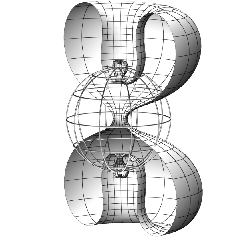
(a) Delaunay surface in $\mathrm{H}^{3}\cup\mathrm{S}^{2}\cup\mathrm{H}^{3}.$ Each of the two ends of this surface of revolution oscillates between the two copies of $\mathrm{H}^{3}$, crossing the ideal boundary infinitely often.

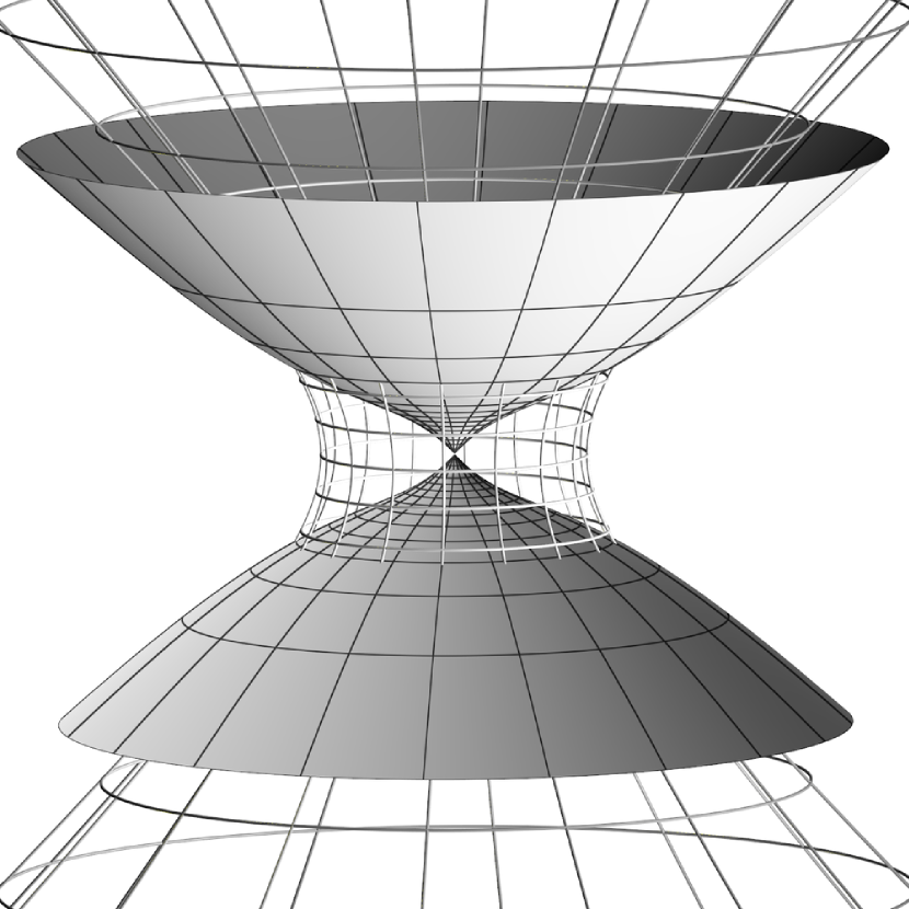
(b) Minimal Delaunay surface in $\mathrm{AdS}_{3}.$ At the cone point (center of image), the profile curve of this surface of revolution crosses the revolution axis and the surface fails to be immersed.

Figure 2.

A less trivial class of surfaces is given by Delaunay surfaces in $\mathrm{H}^{3}$. Minimal Delaunay cylinders in $\mathrm{H}^{3}$ (figure 2(a)) were first described in [3] in terms of their elliptic spectral data. They come in a real 1-dimensional family of geometrically distinct surfaces. On $\mathbb{C}/(2\pi i\mathbb{Z})$, the Hopf differential of a Delaunay cylinder is a constant multiple of $(\mathrm{d}w)^{2}$, and the conformal factor is a solution of the cosh-Gordon equation (remark 1.4). The conformal factor can be given explicitly in terms of the Weierstrass $\wp$-function on a rectangular elliptic curve; see for example [3, 4]. The surface is rotational symmetric, and the conformal factor only depends on one (real) variable and is periodic — but blows up once each period where the surface intersects the ideal boundary at $\infty$ (figure 2(a)).

We consider the Delaunay cylinders parametrized on the two-punctured sphere $\mathbb{C}^{\ast}$, whose Hopf differential is a constant multiple of $(\mathrm{d}z)^{2}/z^{2}$. To construct this 1-dimensional family on the domain $\mathbb{C}^{\ast}$ via the GWR approach take evaluation points

(2.24) $$\lambda_{0}=-\lambda_{1}=1$$

determined by the mean curvature $H=0$ in the last column of table (1.4). The GWR potential on the domain $\mathbb{C}^{\ast}$ is $\mathbbm{i}A\mathrm{d}z/z$ where $A$ is a $z$-independent loop with the following properties (remark 1.8):

• $q\in\mathbb{R}^{\ast}$ is a branch-point of the spectral curve: $\det A(q)=0$;

• intrinsic closing condition: $A=A^{\ast}$; see the third row of (1.2);

• extrinsic closing condition: eigenvalues of $A(\lambda_{0})$ are $\pm\mathbbm{i}/2$.

It follows that the eigenvalues of the frame monodromy around the puncture $z=0$ are $\exp(\pm 2\pi\nu)$ where

(2.25) $$\nu=\tfrac{\mathbbm{i}}{2}\sqrt{\tfrac{(\lambda-q)(-\lambda^{-1}-q)}{q^{2}-1}}.$$

More explicitly, for $\mathrm{H}^{3}$ we may take $A$ to be

(2.26) $$\quad\tfrac{1}{2\sqrt{q^{2}-1}}\begin{bmatrix}0&\lambda^{-1}+q\\ \lambda-q&0\end{bmatrix}$$

constrained by the condition that the term under the square root is positive, i.e., $|q|>1$.

The GWR frame $\Phi$ is based at $z=1$, i.e., $\Phi(1)=\mathbbm{1}$. Hence $\Phi=\exp(\mathbbm{i}A\log z)$.

Theorem 2.3.

The GWR construction applied to the above data gives Delaunay cylinders.

Proof.

The GWR frame for the potential $\xi$ is $\Phi=\exp(\mathbbm{i}A\log z)$. The monodromy of $\Phi$ around the puncture $z=0$ is $M=\exp(2\pi A)$, satisfying the intrinsic closing condition $M^{\ast}=M$ due to the symmetry of $A$, and the extrinsic closing condition (on the cylinder) $M(\lambda_{0})=M(\lambda_{1})=-\mathbbm{1}$ due to the fact that the eigenvalues of $A$ are $\pm\mathbbm{i}/2$ at each evaluation point. Hence the surface closes on $\mathbb{C}^{\ast}$.

To show that the induced surface is a surface of revolution, changing coordinates $x+\mathbbm{i}y=\mathbbm{i}\log z$, then $\Phi=\exp((x+\mathbbm{i}y)A)=\exp(xA)\exp(\mathbbm{i}yA)$. Since $\exp(xA)$ is unitary, then the unitary factor in the Iwasawa decomposition of $\Phi$ is $F(x,\,y)=\exp(xA)G(y)$, where $G$ is the unitary factor of $\exp(\mathbbm{i}yA)$. Hence $F$ is equivariant. Hence the surface $F_{\lambda_{0}}F^{-1}_{\lambda_{1}}$ is equivariant with equivariant action on the profile curve $X=X(y)=G_{\lambda_{0}}G^{-1}_{\lambda_{1}}$ given by

(2.27) $$X\mapsto\exp(xA(\lambda_{0}))X\exp(-xA(\lambda_{1})).$$

This action has closed orbits with period $x\in[0,\,2\pi]$ because the eigenvalues of $A(\lambda_{0})$ and $A(\lambda_{1})$ are $\pm\mathbbm{i}/2$. ∎

Remark 2.4.

It is possible to compute the unitary factor $G$ of $\exp(\mathbbm{i}yA)$ explicitly in terms of elliptic functions. It turns out that $G$ is quasiperiodic in $y$ (i.e., it is equivariant, and the period depends on $q$), and that the Iwasawa decomposition fails twice in each period. On the other hand, using (2.14) it is possible to extend the Delaunay surface to a conformal immersion of the cylinder $\mathbb{C}^{\ast}$ into $\mathrm{S}^{3}$; see also [3, $\S 6$] and figure 2(a).

Remark 2.5.

It is worth noting that the intersection of a Delaunay cylinder with the boundary at infinity is the disjoint union of circles. This follows from the fact that Delaunay cylinders are equivariant. If we restrict to one component of the Delaunay cylinder inside $\mathrm{H}^{3}$ we obtain exactly two boundary circles, which define a Riemann surface of annulus type. It would be interesting to work out in detail the relation between the free parameter $q$ and the modulus of the annulus.

2.3   $n$-noids

An $n$-noid in $\mathbb{R}^{3}$ is a minimal immersion of a $n$ punctured Riemann sphere, each of whose end monodromies has Delaunay eigenvalues, that is, the same eigenvalues as those of a Delaunay cylinder.

In the previous example we have seen that a Delaunay end in $\mathrm{H}^{3}$ cannot be defined on a punctured disk when we consider the surface lying only in $\mathrm{H}^{3}$. We therefore have to modify our definition:

Definition 2.6.

An $n$-noid in $\mathrm{H}^{3}$ is a conformal immersion

(2.28) $$f\colon\mathbb{C}\mathrm{P}^{1}\setminus\{p_{1},\dots,,p_{n}\}\to\mathcal{L}\cong\mathrm{S}^{3}$$

such that

1. the intersection

   (2.29) $$\text{image}(f)\setminus(\mathcal{L}\cap P(e_{4})^{\perp}))=\text{image}(f)\setminus S^{2}=\text{image}(f)\cap(\mathrm{H}^{3}\cup\mathrm{H}^{3})$$

   is a (not necessarily connected) minimal surface;

2. the surface has Delaunay eigenvalues around each end $p_{k}$.

Remark 2.7.

It is necessary to explain the second condition in more detail. In general, if the surface passes through the boundary at infinity, the associated family of flat connections (remark 1.2) does not exist on the $n$-punctured sphere $\mathbb{C}\mathrm{P}^{1}\setminus\{p_{1},\dots,p_{n}\}$ and it is therefore not obvious in which sense one should test the second condition. For example, one should expect that the intersection of $\text{image}(f)\cap(\mathrm{H}^{3}\cup\mathrm{H}^{3})$ around an end $p_{k}$ is defined on a nested union of disjoint topological annuli, and a priori it is unclear why the eigenvalues of the monodromy on all annuli are the same. On the other hand, using condition (1), the surface $f$ is a Willmore surface in $\mathrm{S}^{3}$ and has an associated family of flat $\mathrm{SL}(4,\mathbb{C})$-connections which reduces (in a $\lambda$-dependent way) to the associated family of rank 2 connections of the minimal surface in $\mathrm{H}^{3}$ on the corresponding subset. In this way, it can be shown that the monodromy representation up to conjugation is well-defined; for details see [17].

On the other hand, for minimal surfaces constructed from GWR potentials the monodromies of the potential and the associated family agree up to conjugation, and the eigenvalue condition can therefore be checked directly on the potential.

Example 2.8.

All minimal Delaunay cylinders are 2-noids. In fact, it follows from [3] that these surfaces can be extended through the boundary at infinity to give a (Moebius-)periodic surface into $\mathrm{S}^{3}$ from the two-punctured sphere.

So far we only have numerical evidence of the existence of $n$-noids in $\mathrm{H}^{3}$ (figures 1, 3 and 7). We are therefore forced to give the following weaker definition.

Definition 2.9.

An open $n$-noid in $\mathrm{H}^{3}$ is a conformal minimal immersion of a $n$-holed sphere

(2.30) $$f\colon\mathbb{C}\mathrm{P}^{1}\setminus(D_{1}\cup\cdots\cup D_{n})\to\mathrm{H}^{3}$$

for non-intersecting topological disks $D_{k}\subset\mathbb{C}\mathrm{P}^{1}$, such that the monodromy eigenvalues around each hole $D_{k}$ are the monodromy eigenvalues of a Delaunay cylinder for some $q\in\mathbb{R}$ with $|q|>1$.

Remark 2.10.

Not every $n$-noid in $\mathrm{H}^{3}$ is an open $n$-noid in the above sense. For example, it might be the case that two or more ends of the $n$-noid start in each of the two $\mathrm{H}^{3}$ copies inside the conformal 3-sphere, while the two pieces are joined by a surface which is close to a part of a round sphere. In fact, such examples can be constructed by the methods below. On the other hand, we will construct open $n$-noids in theorem 2.13. We conjecture that those surfaces are $n$-noids in the sense of definition 2.6 (figures 1, 3 and 7).

2.3.1   3-noids

A potential for trinoids is

(2.31) $$\begin{bmatrix}0&\lambda^{-1}\\ f(\lambda)Q&0\end{bmatrix}\mathrm{d}z,$$

where $Q\mathrm{d}z^{2}$ is a holomorphic quadratic differential with three double poles and real quadratic residues, $\lambda_{0},\,\lambda_{0}^{-1}$ are the evaluation points, and for the ambient space $\mathrm{H}^{3}$

(2.32) $$\quad f=(\lambda-1)(\lambda+1).\quad$$

Since at each of its poles the potential is gauge equivalent to a perturbation of a Delaunay potential, by the theory of regular singular points, each monodromy around a puncture has Delaunay eigenvalues. This potential constructs CMC trinoids if the closing conditions of remark 1.8 are satisfied, as shown by the following theorem.

Theorem 2.11.

There exists a real 1-parameter family of GWR potentials on the 3-punctured sphere satisfying the intrinsic and extrinsic closing conditions for minimal surfaces in $\mathrm{H}^{3}$.

The technical proof of the theorem is given in section 4 below.

2.4   Existence of $n$-noid potentials with small necksize

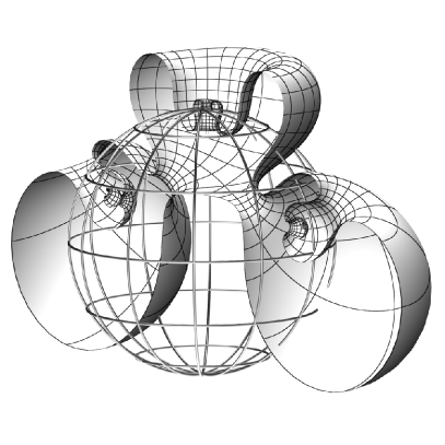
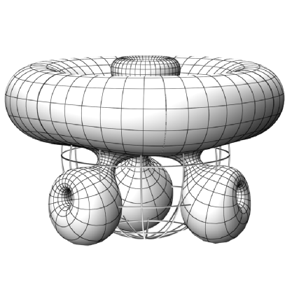
Figure 3. Trinoid and fournoid in $\mathrm{H}^{3}\cup\mathrm{S}^{2}\cup\mathrm{H}^{3}$ with respective cyclic symmetries of orders $2$ and $3$ about the vertical axis. Neither surface is equilateral.

We adopt the techniques of Traizet [33] to prove the existence of open $n$-noids in $\mathrm{H}^{3}$. We conjecture that these surfaces are $n$-noids in the sense of definition 2.9 as well.

In [33], Traizet showed the existence of GWR potentials for constant mean curvature $n$-noids in $\mathbb{R}^{3}$ by deforming the GWR potential of the round sphere. His method of solving the monodromy problem for the intrinsic and extrinsic closing conditions can be easily translated to our setup, with basically identical proofs up to minor changes. Additionally, one can deduce that the Iwasawa factorization works on a subset homeomorphic to a $n$-holed sphere, which yields actually examples of open $n$-noids in $\mathrm{H}^{3}$. A formally similar method of deforming surfaces in $\mathrm{S}^{3}$ and $\mathrm{H}^{3}$ has been introduced in [18] and [16] respectively.

We start with a potential

(2.33) $$\xi_{t}(z):=\begin{bmatrix}0&\lambda^{-1}\mathrm{d}z\\ t(\lambda^{2}+1)\omega(z)\end{bmatrix}$$

where

(2.34) $$\omega=\sum_{k=1}^{n}\bigg{(}\frac{a_{k}}{(z-z_{k})^{2}}+\frac{b_{k}}{z-z_{k}}\bigg{)}\mathrm{d}z.$$

We call $\mathbf{x}=(a_{1},\dots,z_{n})$ the parameter of the potential. Note that in (2.33) we take the evaluation points to be $\lambda_{0}=\mathbbm{i}$ and $\lambda_{1}=-\mathbbm{i}$ in order to have more natural reality conditions. As in [33], we need to allow that the coefficients $a_{k},\,b_{k},\,z_{k}$ are holomorphic functions in $\lambda$, i.e., they are holomorphic on an open neighborhood of the closed unit disk in the $\lambda$-plane. They need to be adjusted for small $t>0$ such that the intrinsic closing condition is satisfied: we want to find for small $t>0$ holomorphic functions $a_{k},\,b_{k},\,z_{k}$, which are close to constant functions (satisfying a constraint related to some balancing formula) , such that the monodromy based at $z=0$ of the potential (2.33) is in the unitary loop group determined by (1.2) corresponding to the symmetric space $\mathrm{H}^{3}$. As we suppose that the functions $z_{k}$ are close enough to constants, the potential is well-defined on a $n$-holed sphere for all $\lambda\in\{\lambda\in\mathbb{C}^{\ast}\mid 0<|\lambda|<1+\epsilon\}$ for some $\epsilon>0$, and the monodromy is computed on this $n$-holed sphere. We call $\mathbf{x}=(t,a_{1},\dots,z_{1},\dots)$ the parameter of the potential, even in the case when $a_{1},\dots,z_{1},\dots$ depend on $\lambda$.

For $\epsilon>0$, we denote by $\mathcal{B}^{\epsilon}$ the Banach space of holomorphic functions on

(2.35) $$\{\lambda\in\mathbb{C}\mid|\lambda|<1+\epsilon\},$$

equipped with the generalized Wiener norm as in [33, $\S$4].

Lemma 2.12.

For $k=1,\dots,n$ let $\tau_{k}\in\mathbb{R}\setminus\{0\}$ and $p_{k}\in\mathbb{C}\setminus(\{0\}\cup\mathrm{S}^{1}$ such that

(2.36) $$0=\sum_{k=1}^{n}\frac{2\tau_{k}\overline{p_{k}}}{1-|p_{k}|^{2}}=\sum_{k=1}^{n}\tau_{k}\frac{1+|p_{k}|^{2}}{1-|p_{k}|^{2}}=\sum_{k=1}^{n}\frac{2\tau_{k}p_{k}}{1-|p_{k}|^{2}}.$$

Then there exists $\epsilon$, $T>0$ and unique smooth maps

(2.37) $$b_{k},z_{k}\colon[0;T[\ \to\ \mathcal{B}^{\epsilon},\quad k=1,\dots,n$$

with

(2.38) $$b_{k}(0)=\frac{2\tau_{k}\overline{p_{k}}}{1-|p_{k}|^{2}},\quad z_{k}(0)=p_{k}$$

for $k=1,\dots,n$, and $z_{k}(0)(0)=p_{k}$ for $k=1,\dots,n$, and a smooth functions $\tau_{k}\colon[0,T[\to\mathbb{R}$ with $\tau_{k}(0)=\tau_{k},$ $k=1,\dots,n$ such that for $t\in[0;T[$ the potential (2.33) with parameter

(2.39) $$\mathbf{x}=(t,\tau_{1},\dots,\tau_{n},a_{n}(t),b_{1}(t),\dots,z_{n}(t))$$

has $\mathrm{H}^{3}$-unitary monodromy at $z=0$.

Proof.

The proof is analogous to the proof of [33, Proposition 3], under the extra assumption that $|p_{k}|\neq 1$ for $k=1,\dots,n$, and using the adapted $\ast$-operator on functions, i.e. $f^{\ast}(\lambda)=\overline{f(-1/\bar{\lambda})}$. The proof that the functions $\tau_{k}$ are independent of $\lambda$ and real-valued can be done similarly to the proof of [33, Proposition 4] by looking at the eigenvalues of the local monodromies. ∎

As a corollary we obtain our main theorem:

Theorem 2.13.

For every $n>1$ there exist open minimal $n$-noids in $\mathrm{H}^{3}$.

Proof.

For $n=2$ we have seen the existence of Delaunay cylinders. For $n\neq 3$ it is easy to see the existence of $n$ pairwise distinct points $p_{k}\in\mathbb{C}^{\ast}$ with $0<|b_{l}|<1$ for $l=1,\dots,n-1$ and $|p_{n}|>1$ and $n$ positive real numbers $\tau_{k}$ satisfying the balancing formula (2.36).

To construct an open minimal $n$-noid we consider for $T>t>0$ the potential provided by Lemma 2.12, and the solution $\Phi$ of

(2.40) $$d\Phi=\Phi\xi_{t};\quad\Phi(0)=\mathbbm{1}.$$

The Iwasawa decomposition (for the real involution corresponding to $\mathrm{H}^{3}$) does exist on an open subset of the loop group $\Lambda\mathrm{SL}_{2}(\mathbb{C})$, containing the constant loop $\mathbbm{1}$. As for $\delta>0$ small enough and $t$ small enough $\xi_{t}$ is arbitrarily close to $\xi_{0}$ on

(2.41) $$\Sigma=\{z\in\mathbb{C}\mid|z|<1-\delta;|z-p_{k}|>\delta\text{ for }k=1,\dots,n-1\}$$

the loop $\Phi(z)$ admits an Iwasawa decomposition on the $n$-holed sphere $\Sigma$, and theorem 1.5 for the evaluation points $\lambda_{0}=\mathbbm{i}$, $\lambda_{1}=-\mathbbm{i}$ provides a minimal surface

(2.42) $$f\colon\Sigma\to\mathrm{H}^{3}.$$

By construction (and for $\delta$ small enough), the monodromies around the holes have Delaunay eigenvalues since at each of its poles the potential is gauge equivalent to a perturbation of a Delaunay potential. ∎

Figure 4 presents an equilateral minimal 16-noid. This is a surfaces with dihedral symmetry. Our numerical experiments show that such surfaces stay embedded for an arbitrary number of ends.

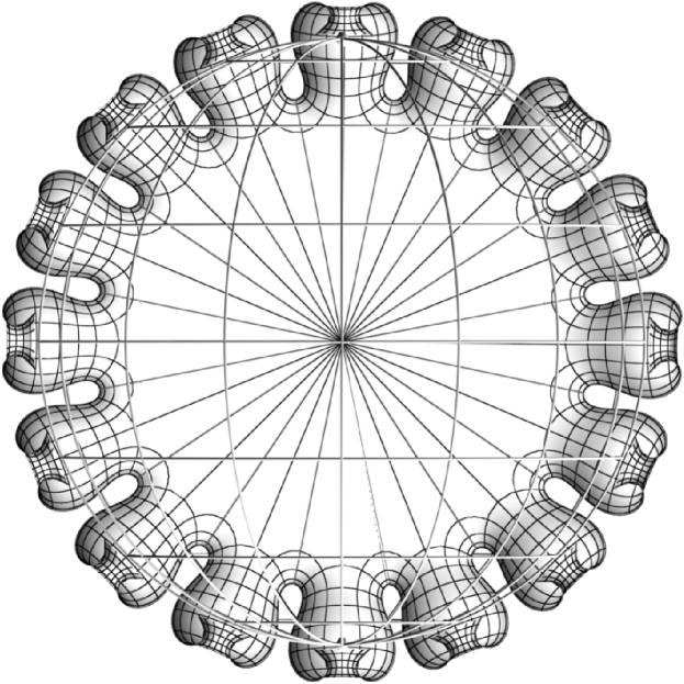
Figure 4. An equilateral minimal 16-noids in $\mathrm{H}^{3}\cup\mathrm{S}^{2}\cup\mathrm{H}^{3}$ with cyclic symmetry of order $16$.

Conjecture 2.14.

There exist embedded minimal $n$-noids in $H^{3}$ for any $n\in\mathbb{N}^{\geq 2}$.

3   Minimal $n$-noids in anti-de Sitter space $\mathrm{AdS}_{3}$

3.1   The lightcone model for $\mathrm{AdS}_{3}$

We set

(3.1) $$\mathrm{AdS}_{3}=\mathrm{SU}_{11}$$

equipped with the natural biinvariant Lorentzian metric associated to the quadratic form given by the trace. As for hyperbolic space, anti-de Sitter space can be defined as the complement of the boundary at infinity

(3.2) $$S_{\infty}=\{\mathbb{R}(x_{0},\,x_{1},\,x_{2},\,x_{3},\,0)\mid x_{0}^{2}+x_{1}^{2}-x_{2}^{2}-x_{3}^{2}=0\}$$

of the lightcone

(3.3) $$\mathcal{L}=\{\mathbb{R}(x_{0},\,x_{1},\,x_{2},\,x_{3},\,x_{4})\mid x_{0}^{2}+x_{1}^{2}-x_{2}^{2}-x_{3}^{2}-x_{4}^{2}=0\}$$

via

(3.4) $$\mathbb{R}(x_{0},\,x_{1},\,x_{2},\,x_{3},\,x_{4})\in\mathcal{L}\setminus S_{\infty}\mapsto\frac{1}{x_{4}}\begin{bmatrix}x_{0}+ix_{1}&x_{2}-ix_{3}\\ x_{2}+ix_{3}&x_{0}-ix_{1}\end{bmatrix}\in\mathrm{SU}_{11}.$$

For visualization, we make use of the stereographic projection

(3.5) $$[x_{0},\,x_{1},\,x_{2},\,x_{3},\,x_{4}]\in\mathcal{L}^{0}\mapsto\frac{1}{x_{0}+x_{4}}(x_{1},\,x_{2},\,x_{3})\in\mathbb{R}^{1,2}$$

defined on

(3.6) $$\mathcal{L}^{0}=\mathcal{L}\setminus\{\mathbb{R}(x_{0},\,x_{1},\,x_{2},\,x_{3},\,-x_{0})\mid x_{1}^{2}-x_{2}^{2}-x_{3}^{2}=0\}.$$

This map is a conformal diffeomorphism onto an open subset of Minkowski space $\mathbb{R}^{1,2}$.

3.2   Basic examples

We first describe some simple surfaces in terms of the GWR approach.

3.2.1   The sphere in $\mathrm{AdS}_{3}$

As in the case of $\mathrm{S}^{3}$ and $\mathrm{H}^{3}$ the easiest example of a GWR potential is given by

(3.7) $$\xi(\lambda)=\begin{bmatrix}0&\lambda^{-1}\\ 0&0\end{bmatrix}dz$$

on the complex plane, with GWR frame

(3.8) $$\Phi(\lambda)=\begin{bmatrix}1&\lambda^{-1}z\\ 0&1\end{bmatrix}.$$

The factorization for $\mathrm{AdS}_{3}$ is given by

(3.9) $$\Phi(\lambda)=F(\lambda)B(\lambda)=\frac{1}{\sqrt{1-z\bar{z}}}\begin{bmatrix}1&\lambda^{-1}z\\ \lambda\bar{z}&1\end{bmatrix}\frac{1}{\sqrt{1-z\bar{z}}}\begin{bmatrix}1&0\\ -\lambda\bar{z}&1-z\bar{z}\end{bmatrix}$$

and taking evaluation points $\lambda_{0}=1$ and $\lambda_{1}=-1$ we obtain

(3.10) $$f=F(1)F(-1)^{-1}=\frac{1}{1-z\bar{z}}\begin{bmatrix}1+z\bar{z}&2z\\ 2\bar{z}&1+z\bar{z}\end{bmatrix}.$$

Restricted to the unit disk $D\subset\mathbb{C}$ this is just a conformally parametrized totally geodesic hyperbolic disk inside $\mathrm{SU}_{11}=\mathrm{AdS}_{3}$ with induced metric

(3.11) $$\frac{1}{1-z\bar{z}}\mathrm{d}z\otimes\mathrm{d}\bar{z}.$$

Remark 3.1.

The surface $f$ is not well-defined on the whole plane $\mathbb{C}$ or projective line, but crosses the ideal boundary at infinity $S_{\infty}$ along the unit circle $\mathrm{S}^{1}\subset\mathbb{C}$. By (3.10) $f$ can be continued on the complement of the closed unit disk as a map into $\mathrm{SU}_{11}$. Again, this phenomena turns out to be typical in the examples below (figures 2(b) and 6).

3.2.2   Minimal planes

Besides the trivial example of the hyperbolic disk, there is an interesting class of minimal surfaces with trivial topology in $\mathrm{AdS}_{3}$ which have been investigated in detail in [2], and are parametrized by null polygonal boundaries. In the special case of regular polygons the Hopf differential is given by a homogeneous polynomial on the complex plane. The metric is rotationally invariant and given by a global solution of the Painlevé III equation.

Analogous to the GWR description [6] of Smyth surfaces in $\mathbb{R}^{3}$ with rotationally symmetric metric [31] these minimal planes can be constructed via the GWR potential of the form

(3.12) $$\begin{bmatrix}0&\lambda^{-1}\\ cz^{n}&0\end{bmatrix}\mathrm{d}z,\quad n\in\mathbb{N},\quad c\in\mathbb{R}$$

for appropriate $c\in\mathbb{R}\setminus\{0\}$. The surface (with initial condition at $z=0$ given by $\mathbbm{1}$) has discrete ambient cyclic symmetry of order $n+2$. The Iwasawa decomposition is global only for one special value $\hat{c}$ (depending on $n$); see for example the detailed investigations in [14]. In figure 5(a) a surface for $n=1$ with $c$ numerically close to $\hat{c}$ is shown. A systematic investigation of this boundary behavior of solutions of the underlying Gauss equation, i.e., the generalized sinh-Gordon equation, on punctured Riemann surfaces with Hopf differentials having higher order poles is carried out in [15], under the name crowned Riemann surfaces.

3.2.3   Delaunay cylinders in $\mathrm{AdS}_{3}$

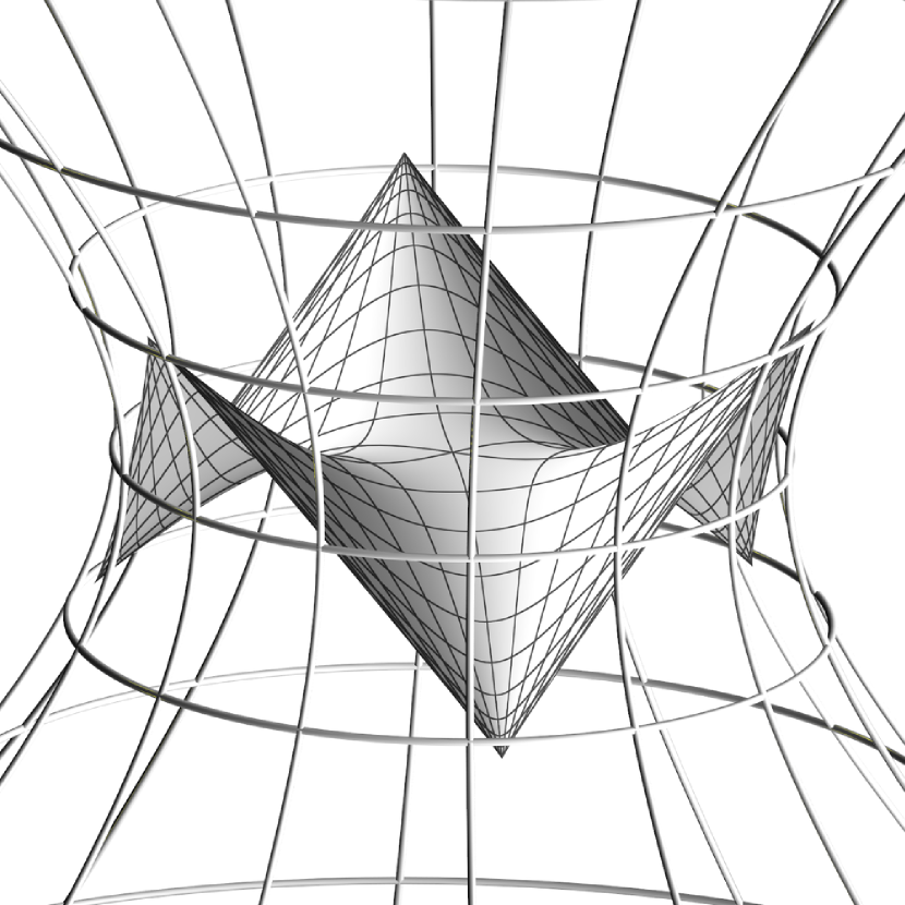
(a) Minimal Smyth surface in $\mathrm{AdS}_{3}$ with cyclic symmetry of order three.

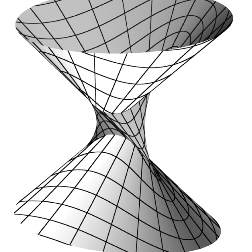
(b) Swallowtail singularity on a minimal surface in $\mathrm{AdS}_{3}$.

Figure 5.

Minimal Delaunay planes in $\mathrm{AdS}_{3}$ have been described in [4] in terms of their elliptic spectral data. By imposing the extrinsic closing condition along the equivariant direction they form a real 1-dimensional family of geometrically distinct surfaces. The conformal factor with respect to the coordinate $\mathrm{d}w$ on $\mathbb{C}/(2\pi\mathbbm{i}\mathbb{Z})$ is a solution of the sinh-Gordon equation with opposite sign as for CMC surfaces in $\mathrm{S}^{3}$ (1.15), and the Hopf differential is a constant multiple of $(\mathrm{d}w)^{2}$. The conformal factor can be given explicitly in terms of the Weierstrass $\wp$-function on a rectangular elliptic curve; see [4]. The surface is rotationally symmetric, and the conformal factor depends only on one (real) variable and is periodic, but blows up once each (intrinsic) period where the surface intersects the ideal boundary at infinity. Moreover, the conformal factor $v^{2}=e^{2u}$ vanishes to second order once in each (intrinsic) period. Geometrically this means that one tangent direction is mapped to a lightlike vector, while the orthogonal tangent direction (with respect to the Riemann surface structure) spans the kernel of the differential of the CMC surface. In the equivariant case, at the singular points, the kernel of the differential of the CMC surface coincides with the kernel of the differential of the conformal factor $v^{2}$, giving us a cone point (figure 2(a)). This phenomena does not happen generally, where a swallowtail like singularity is expected (figure 5(b)).

In the following, we consider the Delaunay cylinders parametrized on the 2-punctured sphere $\mathbb{C}^{\ast}$, where the Hopf differential is a constant multiple of $(\mathrm{d}z)^{2}/z^{2}$. These can be constructed via theorem 1.5 analogously to Delaunay cylinders in $\mathrm{H}^{3}$.

A family of GWR potentials inducing Delaunay surfaces on $\mathbb{C}^{\ast}$ with initial condition $\Phi(1)=\mathbbm{1}$ is

(3.13) $$A\frac{\mathbbm{i}\mathrm{d}z}{z},\quad A=B+B^{\ast},\quad B=\begin{bmatrix}\tfrac{\mathbbm{i}c}{2}&a\lambda^{-1}\\ b&-\tfrac{\mathbbm{i}c}{2}\end{bmatrix},\quad a\in\mathbb{R}^{\ast},\quad b,\,c\in\mathbb{R}.$$

Imposing the extrinsic closing condition with $\lambda_{0}=\mathbbm{i}$, a $1$-parameter family of potentials is given by

(3.14) $$B=\frac{1}{2\sqrt{q^{2}+1}}\begin{bmatrix}\mathbbm{i}\sqrt{2(q^{2}+1)}&\lambda^{-1}+q\\ \lambda+q&-\mathbbm{i}\sqrt{2(q^{2}+1)}\end{bmatrix}\\$$

for $q\in\mathbb{R}$. The meromorphic frame $\Phi$ is based at $z=1$ with $\Phi(1)=\mathbbm{1}$. As in the previous section we obtain:

Theorem 3.2.

The GWR construction applied to the above data gives Delaunay cylinders in $\mathrm{AdS}_{3}$.

An example is shown in figure 2(b).

3.3   $n$-noids in $\mathrm{AdS}_{3}$

We may define $n$-noids and open $n$-noids in $\mathrm{AdS}_{3}$ in an analogous way as for surfaces in $\mathrm{H}^{3}$. We can also adopt Traizet’s construction [33] as done for the case of minimal surfaces in $\mathrm{H}^{3}$ above to prove the existence of open $n$-noids in $\mathrm{AdS}_{3}$. It would be nice to prove that these examples are actually $n$-noids in the strong sense; a proof of this conjecture might build up on the techniques developed in [27].

Theorem 3.3.

For every $n>1$ there exist open minimal $n$-noids in $\mathrm{AdS}_{3}$.

The proof is analogous to the proof of theorem 2.13, taking the appropriate $\ast$-operator on $\mathrm{SL}_{2}(\mathbb{C})$ and on holomorphic functions. Rather than repeating the details of the arguments we give in the next section a general proof of existence of 3-noid potentials for surfaces in $\mathrm{S}^{3}$, $\mathrm{H}^{3}$, $\mathrm{AdS}_{3}$ and $\mathrm{dS}_{3}$.

4   $3$-noids in symmetric spaces

In this last section we extend slightly the class of surfaces and consider CMC surfaces in the symmetric spaces $\mathrm{S}^{3}$, $\mathrm{H}^{3}$, $\mathrm{AdS}_{3}$ and $\mathrm{dS}_{3}$. Recall from section 1 that these can also be described by the GWR approach. We present a general proof of existence for GWR potentials on a 3-punctured sphere, denoted as trinoids in the following.

The main motivation for giving an explicit proof of existence for trinoids is that the so constructed surfaces can be numerically computed and visualized directly (figures 1, 3, 7 and 6). In particular, the proof might help the reader to perform computer experiments via GWR method. Also, in the case of a 3-punctured sphere, the range of end weights $q$ (determined by the quadratic residues at the ends) is more tractable here than in the implicit function theorem proof of theorem 2.13.

The construction of trinoids is particularly simple because the conjugacy class of the monodromy group in this case is determined by the individual conjugacy classes of the generators. In the case of the involution $\lambda\mapsto 1/\overline{\lambda}$ the closing conditions can be read off from the monodromy eigenvalues, which by the theory of regular singular points, can be read off from the potential.

Each pole of our potential will be a Fuchsian singularity which is GWR gauge equivalent to a perturbation of a Delaunay potential. By the theory of regular singular points, each monodromy around a puncture has Delaunay eigenvalues. This potential constructs CMC trinoids if the closing conditions of remark 1.8 are satisfied. The following theorem constructs trinoids in $\mathrm{AdS}_{3}$, $\mathrm{H}^{3}$ with $|H|<1$, and $\mathrm{dS}_{3}$ with $|H|<1$, in analogy to the construction of trinoids in $\mathrm{S}^{3}$ in [30].

To show that the trinoid closes it is necessary to compute a unitarizer $X$ of the monodromy. Unlike the case of $\mathrm{S}^{3}$, for the other spaceforms the unitarizer could fail to have an Iwasawa factorization. Then the frame with unitary monodromy $X\Phi$ likewise fails to have an Iwasawa factorization, and hence does not construct a trinoid. Hence it is necessary to find a unitarizer which has an Iwasawa factorization, or equivalently, a unitarizer in $\Lambda_{+}\mathrm{SL}_{2}(\mathbb{C})$.

To solve the technical problem of the existence of a monodromy unitarizer in $\Lambda_{+}\mathrm{SL}_{2}(\mathbb{C})$ we make the simplifying restriction to isosceles trinoids, for which two of the three end parameters are equal. As seen in theorem 4.3, under this restriction, a diagonal monodromy unitarizer can be computed explicitly via a scalar Birkhoff factorization.

4.1   Real forms

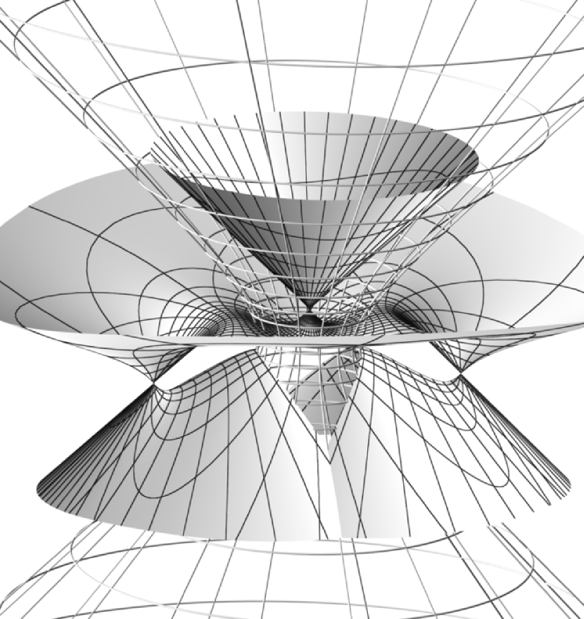
(a) Minimal trinoid in $\mathrm{AdS}_{3}$

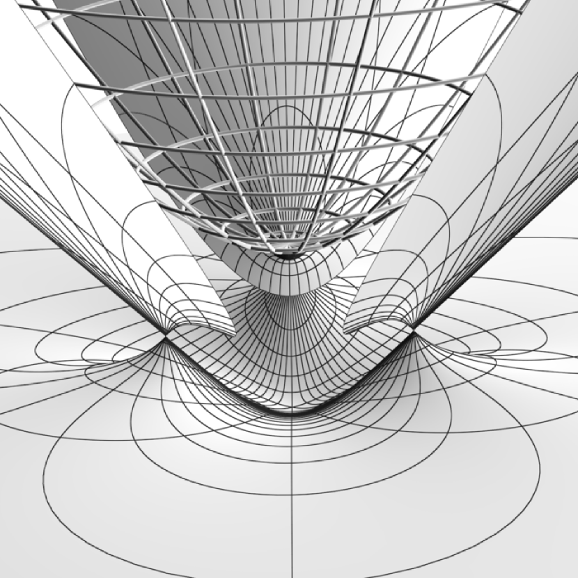
(b) Minimal trinoid in $\mathrm{dS}_{3}$

Figure 6. Minimal trinoids in $\mathrm{AdS}_{3}$ and $\mathrm{dS}_{3}$: three Delaunay half-cylinders glued to a minimal two-sphere (horizontal plane). A swallowtail singularity (figure 5(b)) appears on each Delaunay end.

The four involutions (1.2) on loops $X:\mathrm{S}^{1}\to\mathrm{SL}_{2}\mathbb{C}$ can be indexed by $\delta\in\{\pm 1\}$ and $\epsilon\in\{\pm 1\}$:

(4.1) $$X^{\ast}(\lambda)={{\overline{\eta X(\delta/\overline{\lambda})\eta^{-1}}}^{\mathrm{t}}}^{-1},\quad\eta=\begin{cases}\mathbbm{1}&\text{if $\epsilon=1$}\\ \operatorname{diag}(\mathbbm{i},\,-\mathbbm{i})&\text{if $\epsilon=-1$}.\end{cases}$$

The subgroup of loops $X$ satisfying $X^{\ast}=X$ is the real form for the symmetric spaces as tabulated:

(4.2) $$\begin{array}[]{c|c|c}&\epsilon=1&\epsilon=-1\\ \hline\cr\delta=1&\mathrm{S}^{3}&\mathrm{AdS}_{3}\\ \delta=-1&\mathrm{H}^{3}\ (|H|<1)&\mathrm{dS}_{3}\ (|H|<1)\end{array}$$

A loop $M:\mathrm{S}^{1}\to\mathrm{SL}_{2}\mathbb{C}$ is unitary if $M^{\ast}=M$. A monodromy group is unitarizable if there exists a map $X:\mathcal{D}_{+}\to\mathrm{SL}_{2}\mathbb{C}$ such that for each $M$ in the group $XMX^{-1}$ extends holomorphically to $\mathrm{S}^{1}$ and is unitary.

For scalar loops define

(4.3) $$f^{\ast}(\lambda)=\overline{f(\delta/\overline{\lambda})}.$$

4.2   Trinoids potentials

A potential for trinoids is

(4.4) $$o\begin{bmatrix}0&\lambda^{-1}\\ f(\lambda)Q&0\end{bmatrix}\mathrm{d}z,$$

where $Q\,\mathrm{d}z^{2}$ is a holomorphic quadratic differential with three double poles and real quadratic residues, $f$ satisfying $(f/\lambda)^{\ast}=f/\lambda$ is

(4.5a) $$\mathrm{S}^{3}\text{ and }\mathrm{AdS}_{3} :\quad f=(\lambda-\lambda_{0})(\lambda-\lambda_{0}^{-1}),\quad\lambda_{0}\in\mathrm{S}^{1}\setminus\{\pm 1\}$$

(4.5b) $$\mathrm{H}^{3}\text{ and }\mathrm{dS}_{3} :\quad f=(\lambda-\lambda_{0})(\lambda+\lambda_{0}^{-1}),\quad\lambda_{0}\in\mathbb{R}\setminus\{0\},$$

and $\lambda_{0},\,\lambda_{0}^{-1}$ are the evaluation points $\lambda_{0},\lambda_{1}$ are determined by

(4.6) $$\mathrm{S}^{3}\text{ and }\mathrm{AdS}_{3}:\ \lambda_{1}=1/\lambda_{0}\in\mathrm{S}^{1}\setminus\{\pm 1\};\quad\quad\mathrm{H}^{3}\text{ and }\mathrm{dS}_{3}:\ \lambda_{1}=-1/\lambda_{0}\in\mathbb{R}^{\ast}.$$

For isosceles trinoids choose ends $z=1,\,-1,\,\infty$ and

(4.7) $$Q=\frac{4a+b(z^{2}-1)}{{(z^{2}-1)}^{2}}$$

satisfying $\operatorname*{qres}_{z=\pm 1}Q\,\mathrm{d}z^{2}=a$ and $\operatorname*{qres}_{z=\infty}Q\,\mathrm{d}z^{2}=b$.

4.3   Unitarization

The isosceles trinoid potential (4.4)–(4.7) has symmetries

(4.8a) $$\sigma^{\ast}\xi(\lambda)=\xi(\lambda).g_{1}\quad\sigma(z)=-z,\quad g_{1}=\operatorname{diag}(\mathbbm{i},\,-\mathbbm{i})$$

(4.8b) $$\overline{\tau^{\ast}\xi(\delta/\overline{\lambda})}=\xi(\lambda).g_{2},\quad\tau(z)=\overline{z},\quad g_{2}=\operatorname{diag}(\sqrt{\delta}/\lambda,\,\lambda/\sqrt{\delta}).$$

Let $M_{0}$ and $M_{1}$ be the monodromies around $z=1$ and $z=-1$ respectively, with basepoint $\Phi(0)=\mathbbm{1}$. The symmetries of the potential imply

(4.9) $$M_{0}=\begin{bmatrix}r&p\lambda\\ -q\lambda^{-1}&r^{\ast}\end{bmatrix},\quad M_{1}=\begin{bmatrix}r&-p\lambda\\ q\lambda^{-1}&r^{\ast}\end{bmatrix}$$

for some holomorphic functions $p,\,q,\,r:\mathbb{C}^{\ast}\to\mathbb{C}$ satisfying $rr^{\ast}+pq=1$ and

(4.10) $$p^{\ast}=\delta p\quad\text{and}\quad q^{\ast}=\delta q.$$

Lemma 4.1.

If $q/p^{\ast}$ in (4.9) has a Birkhoff factorization

(4.11) $$q/p^{\ast}=\delta\epsilon x_{+}^{\ast}x_{+},\quad x_{+}:\mathcal{D}_{+}\to\mathbb{C}^{\ast}$$

then $M_{0}$ and $M_{1}$ are unitarizable in the sense of (4.1).

Proof.

If $q/p^{\ast}=\delta\epsilon x_{+}^{\ast}x_{+}$, then $x_{+}:\mathcal{D}_{+}\to\mathbb{C}^{\ast}$ has a single-valued square root $\mathcal{D}_{+}\to\mathbb{C}^{\ast}$, so $X:=\operatorname{diag}(\sqrt{x_{+}},\,1/\sqrt{x_{+}})$ is a single-valued map $\mathcal{D}_{+}\to\mathrm{SL}_{2}(\mathbb{C})$. Then

(4.12) $$P_{0}:=XM_{0}X^{-1}=\begin{bmatrix}r&s\\ -\epsilon s^{\ast}&r^{\ast}\end{bmatrix},\quad P_{1}:=XM_{1}X^{-1}=\begin{bmatrix}r&-s\\ \epsilon s^{\ast}&r^{\ast}\end{bmatrix},\quad s:=px_{+}\lambda$$

extend holomorphically to $\mathrm{S}^{1}$ and satisfy $P_{0}=P_{0}^{\ast}$ and $P_{1}=P_{1}^{\ast}$ in the sense of (4.1). ∎

4.4   Scalar Birkhoff factorization

To unitarize the trinoid monodromy via lemma 4.1 we need a more detailed analysis of the scalar Birkhoff factorization. With $\mathrm{P}^{1}=\mathcal{D}_{+}\sqcup\mathrm{S}^{1}\sqcup\mathcal{D}_{-}$,

(4.13) $$\mathcal{D}_{+}:=\{\lambda\in\mathbb{C}\mid|\lambda|<1\}\quad\mathcal{D}_{-}:=\{\lambda\in\mathbb{C}\mid|\lambda|>1\}\cup\{\infty\}$$

let

(4.14a) $$\Lambda =\{\text{real analytic loops on $\mathrm{S}^{1}\to\mathbb{C}^{\ast}$}\}$$

(4.14b) $$\Lambda_{+} =\{f\in\Lambda\mid\text{$f$ is the boundary of a holomorphic map $\mathcal{D}_{+}\to\mathbb{C}^{\ast}$}\}$$

(4.14c) $$\Lambda_{-} =\{f\in\Lambda\mid\text{$f$ is the boundary of a holomorphic map $\mathcal{D}_{-}\to\mathbb{C}^{\ast}$}\}.$$

1. By [25], every loop $f\in\Lambda$ has a unique Birkhoff factorization

(4.15a) $$f=c\lambda^{n}f_{-}f_{+},\quad n\in\mathbb{Z},\quad c\in\mathbb{C}^{\ast},\quad$$

(4.15b) $$f_{+}\in\Lambda_{+},\quad f_{-}\in\Lambda_{-},\quad f_{+}(0)=1,\quad f_{-}(\infty)=1.$$

Let star be as in (4.3) for either choice of $\delta\in\{\pm 1\}$.

2. If $f\in\Lambda$ satisfies $f=f^{\ast}$, then $f$ has a unique Birkhoff factorization

(4.16) $$f=\epsilon f_{+}^{\ast}f_{+},\quad\epsilon\in\{\pm 1\},\quad f_{+}\in\Lambda_{+},\quad f_{+}(0)\in\mathbb{R}_{+}.$$

This defines an homomorphism

(4.17) $$\operatorname{sign}:\{f\in\Lambda\mid f=f^{\ast}\}\to\{\pm 1\},\quad f\mapsto\epsilon.$$

A meromorphic loop on $\mathrm{S}^{1}$ is meromorphic in a neighborhood of $\mathrm{S}^{1}$. Let $\Lambda^{\ast}$ be the subgroup of meromorphic loops on $\mathrm{S}^{1}$

(4.18) $$\Lambda^{\ast}=\{\text{$f\mid f^{\ast}=f$ and $\mathrm{div}_{\mathrm{S}^{1}}f$ even}\},$$

where $\mathrm{div}_{\mathrm{S}^{1}}f$ even means that the order of each zero and pole of $f$ on $\mathrm{S}^{1}$ is even.

3. Every $f\in\Lambda^{\ast}$ has a unique Birkhoff factorization

(4.19) $$f=\epsilon f_{+}^{\ast}f_{+},\quad\epsilon\in\{\pm 1\},\quad\mathrm{div}_{\mathrm{S}^{1}}f_{+}=\tfrac{1}{2}\mathrm{div}_{\mathrm{S}^{1}}f$$

where $f_{+}$ is the boundary of a holomorphic map $\mathcal{D}_{+}\to\mathbb{C}^{\ast}$. This extends the homomorphism (4.17) to an homomorphism

(4.20) $$\operatorname{sign}:\Lambda^{\ast}\to\{\pm 1\},\quad f\mapsto\epsilon.$$

4. For every meromorphic loop $f$ on $\mathrm{S}^{1}$ with $f=f^{\ast}$

(4.21) $$\operatorname{sign}[f^{2}]=1.$$

4.5   The trace polynomial

Given a monodromy representation $M_{0},\,M_{1},\,M_{2}$ with $M_{0}M_{1}M_{2}=\mathbbm{1}$ on the three-punctured sphere, define the polynomial [13]

(4.22) $$\varphi=1-t_{0}^{2}-t_{1}^{2}-t_{2}^{2}+2t_{0}t_{1}t_{2},\quad t_{k}=\tfrac{1}{2}\operatorname{tr}(M_{k}),\quad k\in\{0,\,1,\,2\}.$$

The trace polynomial vanishes precisely where the monodromy representation is reducible. In the case of the involution $\lambda\mapsto 1/\overline{\lambda}$, if the halftraces are in $(-1,\,1)$, then the monodromy is $\mathrm{SU}_{2}$-unitarizable if $\varphi>0$ and $\mathrm{SU}_{11}$-unitarizable if $\varphi<0$.

For the trinoid potential (4.4) with quadratic residues $(q_{0},\,q_{1},\,q_{2})\in\mathbb{R}^{3}$ of $Q$, and $f$ as in (4.5),

(4.23) $$t_{k}=\cos(2\pi\nu_{k}),\quad\nu_{k}=\tfrac{1}{2}-\tfrac{1}{2}\sqrt{1+q_{k}\kappa},\quad\kappa=4\lambda^{-1}f(\lambda),\quad k\in\{0,\,1,\,2\}.$$

The function $\kappa:\mathrm{S}^{1}\to\mathbb{C}$ satisfies $\kappa^{\ast}=\kappa$.

The trace polynomial $\varphi:\mathrm{S}^{1}\to\mathbb{C}$ for the monodromies of the trinoid potential satisfies $\varphi^{\ast}=\varphi$. Putting together (4.22) and (4.23), its series expansion in $\kappa$ at $\kappa=0$ is

(4.24) $$\varphi(\kappa)=c\kappa^{4}+\mathrm{O}(\kappa^{5}),\quad c=\frac{\pi^{4}}{64}(q_{0}+q_{1}+q_{2})(-q_{0}+q_{1}+q_{2})(q_{0}-q_{1}+q_{2})(q_{0}+q_{1}-q_{2}).$$

Lemma 4.2.

Choose $(q_{0},\,q_{1},\,q_{2})\in\mathbb{R}^{3}$ with $c\neq 0$. For $s$ in a small enough interval $(0,\,s_{0})$, $\varphi_{sq}\in\Lambda^{\ast}$ and $\operatorname{sign}[\varphi_{sq}]=\operatorname{sign}(c)$.

Proof.

From the series expansion (4.24),

(4.25) $$|\varphi_{q}/\kappa^{4}-c|<|c/2|\quad\text{for all}\quad|\kappa|<\kappa_{0}.$$

Let $m=1+\max_{\lambda\in\mathrm{S}^{1}}|\kappa(\lambda)|$. Then for all $|\kappa|<m$ and $s\in(0,\,\kappa_{0}/m)$, we have $|s\kappa|<\kappa_{0}$, so

(4.26) $$|\varphi_{sq}(\kappa)/\kappa^{4}-c|=|\varphi_{q}(s\kappa)/\kappa^{4}-c|<|c/2|$$

Hence $\varphi_{sq}/\kappa^{4}$ maps $\mathrm{S}^{1}$ into the disk centered at $c$ with radius $|c/2|$. This implies that $\varphi_{sq}$ has no zeros on $\mathrm{S}^{1}$, except at the zeros of $\kappa$ in the case $\kappa$ has zeros on $\mathrm{S}^{1}$. Since these zeros are of order $4$, then $\varphi\in\Lambda^{\ast}$.

Since $\operatorname{sign}(c)\varphi_{sq}/\kappa^{4}$ takes values in the open right halfplane, it has a single-valued square root $f:\mathrm{S}^{1}\to\mathbb{C}^{\ast}$ satisfying $f^{\ast}=f$. By (4.21), $\operatorname{sign}[\varphi_{sq}]=\operatorname{sign}(c)\operatorname{sign}[\kappa^{4}f^{2}]=\operatorname{sign}(c)$. ∎

In the case of isosceles trinoids, for which $(q_{0},\,q_{1},\,q_{2})=(a,\,a,\,b)$ with $a$, $b$ as in (4.7), then $c=\frac{\pi^{4}}{64}b^{2}(4a^{2}-b^{2})$, so $\operatorname{sign}[\varphi]=+1$ in a subregion of $\{|b|<2|a|\}$. and $\operatorname{sign}[\varphi]=-1$ in a subregion of $\{|b|>2|a|\}$.

4.6   Trinoids

Theorem 4.3.

For each of the four symmetric spaces tabulated in (4.2) there exists a two real parameter family of conformal CMC isosceles trinoid potentials satisfying the closing conditions with prescribed mean curvature $H$.

Proof.

Choose a symmetric space, $\epsilon\in\{\pm 1\}$ and $\delta\in\{\pm 1\}$ as tabulated in (4.2), and a isosceles trinoid potential (4.4)–(4.7).

By lemma 4.2, there exists a subregion of $\{(a,\,b)\in\mathbb{R}^{2}\}$ with $(a,\,b)$ as in (4.7), in which $\varphi\in\Lambda^{\ast}$ and $\operatorname{sign}[\varphi]=\delta\epsilon$.

Let $M_{0}$ and $M_{1}$ be the monodromies of the meromorphic frame $\Phi$ based at $\Phi(0)=\mathbbm{1}$ as in (4.9). The respective halftraces $t_{0},\,t_{1},\,t_{2}$ of $M_{0},\,M_{1},\,M_{2}=M_{1}^{-1}M_{0}^{-1}$ are

(4.27) $$t_{0}=t_{1}=\tfrac{1}{2}(r+r^{\ast})\quad\text{and}\quad t_{2}=\tfrac{1}{2}(r^{2}-2pq+{r^{\ast}}^{2})$$

so the trace polynomial (4.22) is

(4.28) $$\varphi={(\mathbbm{i}(r-r^{\ast}))}^{2}pq.$$

Since $\varphi\in\Lambda^{\ast}$ and ${(\mathbbm{i}(r-r^{\ast}))}^{2}\in\Lambda^{\ast}$, then $pq\in\Lambda^{\ast}$. Since $p^{\ast}p\in\Lambda^{\ast}$ then $q/p^{\ast}=(pq)/(p^{\ast}p)\in\Lambda^{\ast}$. By (4.21) $\operatorname{sign}[{(\mathbbm{i}(r-r^{\ast}))}^{2}]=1$ and $\operatorname{sign}[p^{\ast}p]=1$, so

(4.29a) $$\operatorname{sign}[q/p^{\ast}] =\operatorname{sign}[(pq)/(p^{\ast}p)]=\operatorname{sign}[pq]\operatorname{sign}[p^{\ast}p]=\operatorname{sign}[pq]$$

(4.29b) $$=\operatorname{sign}[{(\mathbbm{i}(r-r^{\ast}))}^{2}]\operatorname{sign}[pq]=\operatorname{sign}[\varphi]=\delta\epsilon.$$

By the definition of $\operatorname{sign}$, $p/q^{\ast}$ has a factorization $p/q^{\ast}=\delta\epsilon x_{+}^{\ast}x_{+}$, where $x_{+}:\mathcal{D}_{+}\to\mathbb{C}^{\ast}$. By lemma 4.1 there exists a unitarizer $X$ of the monodromy in the sense of (4.1).

By theorem 1.5 the immersion induced by $X\Phi$ via $r$-Iwasawa factorization is conformal and CMC, and by remark 1.8 it closes around each of its three Delaunay ends. ∎

Remark 4.4.

1. In the case of $\mathrm{S}^{3}$ theorem 4.3 reconstructs a two-dimensional subfamily of the three-dimensional family of trinoids constructed in [30] without the isosceles constraint.

2. In the other three symmetric spaces, where the Iwasawa factorization can leave the big cell, the domain of the trinoids constructed by theorem 4.3 is not known, but numerical experiments indicate that in general the whole punctured Riemann sphere is mapped into the light cone, intersecting the ideal boundary along curves (figures 1, 3, 7 and 6).

3. Noids with more than three ends can be constructed using a cyclic branched cover of the Riemann sphere (figures 1 and 3).

4.7   Dressing

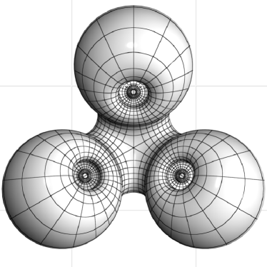
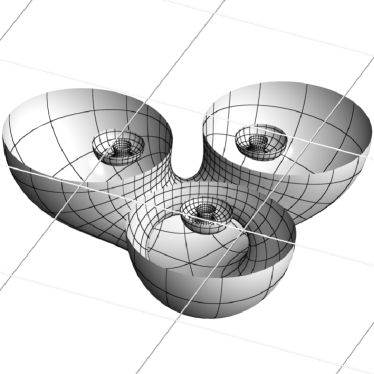
Figure 7. Two views of an equilateral minimal trinoid in $\mathrm{H}^{3}\cup\mathrm{S}^{2}\cup\mathrm{H}^{3}$ stereographically projected to $\mathbb{R}^{3}$ via the Poincaré halfspace model. The cutaway view (right) shows the intersection of the surface with the ideal boundary along nested topological circles.

By theorem 4.3 we can construct equilateral trinoids in $\mathrm{dS}_{3}$ (figure 6(b)), and isosceles non-equilateral trinoids in $\mathrm{H}^{3}$ (figure 3). In this section we construct equilateral trinoids in $\mathrm{H}^{3}$ (figure 1) by dressing equilateral trinoids in $\mathrm{dS}_{3}$. The dressing action interchanges the real forms for $\mathrm{dS}_{3}$ and $\mathrm{H}^{3}$.

More explicitly, the dressing action of a loop $g$ (defined on an a circle of radius $r\in(0,\,1]$) on a frame $F$, written $g\operatorname{\#}F$, is by definition the $r$-unitary factor of $gF$ of its $r$-Iwasawa factorization. In analogy to [32] we take $g$ to be a diagonal simple factor

(4.30) $$g=\operatorname{diag}(p^{1/2},\,p^{-1/2}),\quad p=\frac{\lambda-\mu}{\overline{\mu}\lambda+1},\quad p^{\ast}=-\frac{1}{p}$$

on an $r$-circle, $r<|\mu|$.

Lemma 4.5.

Diagonal simple factor dressing $F\mapsto g\operatorname{\#}F$ interchanges the real form for $\mathrm{dS}_{3}$ with the real form for $\mathrm{H}^{3}$.

Proof.

The dressing action of the simple factor $g$ on a frame $F$ in the real form for $\mathrm{dS}_{3}$ is computed explicitly and algebraically as

(4.31) $$g\operatorname{\#}F=gFk^{-1}g^{-1},\quad k=\tfrac{1}{\sqrt{{|u|}^{2}-{|v|}^{2}}}\big{[}\begin{smallmatrix}u&\overline{v}\\ v&\overline{u}\end{smallmatrix}\big{]},\quad\big{[}\begin{smallmatrix}u\\ v\end{smallmatrix}\big{]}=F^{-1}(\mu)\ell,\quad\ \ell=\big{[}\begin{smallmatrix}1\\ 0\end{smallmatrix}\big{]}.$$

We have

(4.32) $$Fk^{-1}=\begin{bmatrix}s&t\\ t^{\ast}&s^{\ast}\end{bmatrix}\quad\Longrightarrow\quad g\operatorname{\#}F=gFk^{-1}g^{-1}=\begin{bmatrix}s&tp\\ t^{\ast}p^{\ast}&s^{\ast}\end{bmatrix}.$$

Hence $g\operatorname{\#}F$ is in the real form for $\mathrm{H}^{3}$. The proof for the other direction is the same except for a sign change. ∎

Theorem 4.6.

There exists a real $1$-parameter family of equilateral trinoids in $\mathrm{H}^{3}$ for each mean curvature $|H|<1$ (figure 1).

Proof.

Let $F$ be a unitary frame for a trinoid in the $1$-parameter family of equilateral trinoids in $\mathrm{dS}_{3}$ with specified mean curvature $|H|<1$ (theorem 4.3). The dressed frame $g\operatorname{\#}F$ is in the real form for $\mathrm{H}^{3}$ (lemma 4.5) so it satisfies the intrinsic closing condition for $\mathrm{H}^{3}$.

To satisfy the extrinsic closing condition we choose the simple factor $g$ as follows. The subset of the $\lambda$ plane along which the monodromy group of $F$ is reducible is the zero set of the trace polynomial $\varphi$ (4.22). With $t$ the halftrace of the monodromy of $F$ around each end, we have $\varphi={(1-t)}^{2}(1+2t)$ with zero set

(4.33) $$\big{\{}\mu\in\mathbb{C}^{\ast}\mid\tfrac{1}{2}-\tfrac{1}{2}\sqrt{1+4q\mu^{-1}f(\mu)}\in\mathbb{Z}/3\big{\}},\quad\text{$f$ as in~{}\eqref{eq:trinoid-f2}},$$

a discrete subset of $\mathbb{C}^{\ast}$ which accumulates at $0$ and $\infty$. Using (4.9) and (4.28), $\mu$ can be found in this zero set away from the evaluation points such that $\ell$ is a common eigenvalue of the monodromy group. This choice of $\mu$ implies that the monodromy of $g\operatorname{\#}F$ is $gMg^{-1}$, where $M$ is a monodromy of $F$ (in analogy to [20] for noids in $\mathbb{R}^{3}$). Hence $g\operatorname{\#}F$ satisfies the extrinsic closing conditions for $\mathrm{H}^{3}$, so it is the frame for an equilateral trinoid in $\mathrm{H}^{3}$. ∎

Remark 4.7.

The GWR construction of trinoids (theorem 4.3) is as follows:

1. In terms of a potential (4.4) on the three-punctured sphere, compute a dressing $C$ which unitarizes the monodromy group of the corresponding holomorphic frame $\Phi$ based at $\Phi(z_{0})=\mathbbm{1}$.

2. Show that the dressed holomorphic frame $C\Phi$ is in the big cell of the Iwasawa decomposition in some subregion of the domain.

3. Construct a CMC immersion of that subregion into $\mathrm{H}^{3}$ via the evaluation formula (1.3) applied to the unitary Iwasawa factor of $C\Phi$.

Following this program with gauge equivalent trinoid potentials, Kobayashi in [21, Theorem 4.1] gives an incomplete construction of equilateral trinoids in $\mathrm{H}^{3}$ with mean curvature $|H|<1$, failing to address step (2). Our theorem 4.6 fills this gap by constructing a dressing $C$ in the loop group $\Lambda_{+}\mathrm{SL}_{2}(\mathbb{C})$. Thus $C\Phi$ is in the big cell of the Iwasawa decomposition at, and hence in a neighborhood of the basepoint $z_{0}$. Moreover, it follows from Theorem 2.13 that for small necksizes $C\Phi$ is in the big cell of the Iwasawa decomposition on the 3-holed sphere obtained by removing 3 discs around the punctures of the 3-punctured sphere.

Dorfmeister, Inoguchi and Kobayashi further state without proof in [9, §10.5] that the theorem of Kobayashi mentioned above constructs CMC immersions of the three-punctured sphere into $\mathrm{H}^{3}$. On the contrary, in light of the numerical evidence of figures 1, 3, 7 and 6, we conjecture that in analogy to 2-noids (Delaunay surfaces), the incompletely constructed trinoids in [21] map the three-punctured sphere not into $\mathrm{H}^{3}$ but into $\mathrm{H}^{3}\cup\mathrm{S}^{2}\cup\mathrm{H}^{3}$.

References

• [1] L. Alday and J. Maldacena, Gluon scattering amplitudes at strong coupling, J. High Energy Phys. (2007), no. 6, 064, 26.
• [2] by same author, Null polygonal Wilson loops and minimal surfaces in anti-de-Sitter space, J. High Energy Phys. (2009), no. 11, 082, 59.
• [3] M. Babich and A. I. Bobenko, Willmore tori with umbilic lines and minimal surfaces in hyperbolic space, Duke Math. J. 72 (1993), no. 1, 151–185.
• [4] I. Bakas and G. Pastras, On elliptic string solutions in $\rm AdS_{3}$ and $\rm dS_{3}$, J. High Energy Phys. (2016), no. 7, 070.
• [5] A. I. Bobenko, Surfaces of constant mean curvature and integrable equations, Uspekhi Mat. Nauk 46 (1991), no. 4 (280), 3–42; translation in Russian Math. Surveys 46 (1991), no. 4, 1–45.
• [6] A. I. Bobenko, A. R. Its, The Painlevé III Equation and the Iwasawa Decomposition, Manuscripta Math. 87 (1995), no. 3, 369–377.
• [7] D. Brander, W. Rossman, and N. Schmitt, Holomorphic representation of constant mean curvature surfaces in Minkowski space: consequences of non-compactness in loop group methods, Adv. Math. 223 (2010), no. 3, 949–986.
• [8] F. Burstall, F. Pedit, and U. Pinkall, Schwarzian derivatives and flows of surfaces, Differential geometry and integrable systems (Tokyo, 2000), Contemp. Math., vol. 308, Amer. Math. Soc., Providence, RI, 2002, pp. 39–61.
• [9] J. Dorfmeister, J. Inoguchi, and S. Kobayashi, Constant mean curvature surfaces in hyperbolic 3-space via loop groups, J. Reine Angew. Math. 686 (2014), 1–36.
• [10] J. Dorfmeister, F. Pedit, and H. Wu, Weierstrass type representation of harmonic maps into symmetric spaces, Comm. Anal. Geom. 6 (1998), no. 4, 633–668.
• [11] N. Drukker, D. Gross, and H. Ooguri, Wilson loops and minimal surfaces, Phys. Rev. D (3) 60 (1999), no. 12, 125006, 20.
• [12] P. Fonda, L. Giomi, A. Salvio, and E. Tonni, On shape dependence of holographic mutual information in ${\rm AdS}_{4}$, J. High Energy Phys. (2015), no. 2, 005, front matter+50.
• [13] W. Goldman, Topological components of spaces of representations, Invent. Math. 93 (1988), no. 3, 557–607.
• [14] M. Guest, A. Its, and C. Lin, Isomonodromy aspects of the $\mathrm{tt}^{\ast}$ equations of Cecotti and Vafa III. Iwasawa factorization and asymptotics, arXiv:1707.00259, 2018.
• [15] S. Gupta, Harmonic maps and wild Teichmüller spaces, arXiv:1708.04780, 2018.
• [16] L. Heller and S. Heller, Higher solutions of Hitchin’s self-duality equations, arXiv:1801.02402, 2018.
• [17] L. Heller, S. Heller, and Ch. Ndiaye, Constrained Willmore minimizers, preprint, 2018.
• [18] L. Heller, S. Heller, and N. Schmitt, Navigating the space of symmetric CMC surfaces, J. Differential Geom. 110 (2018), no. 3, 413–455.
• [19] N. Hitchin, The self-duality equations on a Riemann surface, Proc. London Math. Soc. (3) 55 (1987), no. 1, 59–126.
• [20] M. Kilian, N. Schmitt, and I. Sterling, Dressing CMC $n$-noids, Math. Z. 246 (2004), no. 3, 501–519.
• [21] S. Kobayashi, Totally symmetric surfaces of constant mean curvature in hyperbolic 3-space, Bull. Aust. Math. Soc. 82 (2010), no. 2, 240–253.
• [22] by same author, Real forms of complex surfaces of constant mean curvature, Trans. Amer. Math. Soc. 363 (2011), no. 4, 1765–1788.
• [23] J. Maldacena, The large $N$ limit of superconformal field theories and supergravity, Adv. Theor. Math. Phys. 2 (1998), no. 2, 231–252.
• [24] Y. Ogata, The DPW method for constant mean curvature surfaces in 3-dimensional Lorentzian spaceforms, with applications to Smyth type surfaces, Hokkaido Math. J. 46 (2017), no. 3, 315–350.
• [25] A. Pressley and G. Segal, Loop groups, Oxford Mathematical Monographs, The Clarendon Press, Oxford University Press, New York, 1986, Oxford Science Publications.
• [26] A. Quintino, Constrained Willmore surfaces, Ph.D. thesis, University of Bath, 2009, arXiv:0912.5402.
• [27] T. Raujouan, On Delaunay ends in the DPW method, arXiv:1710.00768, 2018.
• [28] S.-J.. Rey and J.-T. Yee, Macroscopic strings as heavy quarks: large-$N$ gauge theory and anti-de Sitter supergravity, Eur. Phys. J. C Part. Fields 22 (2001), no. 2, 379–394.
• [29] K. Sakai and Y. Satoh, Constant mean curvature surfaces in ${\rm AdS}_{3}$, J. High Energy Phys. (2010), no. 3, 077, 18.
• [30] N. Schmitt, M. Kilian, S. Kobayashi, and W. Rossman, Unitarization of monodromy representations and constant mean curvature trinoids in 3-dimensional space forms, J. Lond. Math. Soc. (2) 75 (2007), no. 3, 563–581.
• [31] B. Smyth, A generalization of a theorem of Delaunay on constant mean curvature surfaces, Statistical thermodynamics and differential geometry of microstructured materials (Minneapolis, MN, 1991), IMA Vol. Math. Appl., vol. 51, Springer, New York, 1993, pp. 123–130.
• [32] C. Terng and K. Uhlenbeck, Bäcklund transformations and loop group actions, Comm. Pure Appl. Math. 53 (2000), no. 1, 1–75.
• [33] M. Traizet, Construction of constant mean curvature $n$-noids using the DPW method, arXiv:1709.00924, 2017.