Unusual broadening of wave packets on lattices

Abstract

The broadening of one-dimensional Gaussian wave packets is presented in all textbooks on quantum mechanics. It is used as an example to elucidate Heisenberg’s uncertainty relation. The behaviour on a lattice is drastically different if the amplitude and (or) phase of the wave packet varies on the scale of the lattice constant. Important examples are very narrow wavepackets or wavepackets with an average velocity comparable to the maximum velocity on the lattice. Analytical and numerical results for the time dependence of wave packets on a one-dimensional lattice are presented. The long-time limit of the shape of the wave packet is discussed.

I Introduction

Even before treating how the probability amplitudes in quantum mechanics vary in continuous space Richard Feynman Feynman in volume III of his famous “Lectures on Physics” addresses what happens if one puts a single electron on a line of atoms. He arrives at the one-dimensional time independent Schödinger equation by studying the limit where the lattice constant $a$ goes to zero. The one-dimensional model studied by Feynman is usually called the “nearest neighbour tight-binding model” and is treated in solid state physics textbooks.AM More recently in the field of quantum computing this model is called a “continuous time quantum walk”. Farhi Here the solid state physics point of view is taken.

Feynman discusses the dynamics of wave packets on the lattice and shows that if they have a predominant wave number $k_{0}$ they move through the lattice with the group velocity $d\omega/dk$. In a footnote he adds “Provided we do not try to make the packet too narrow”. It is one goal of this paper to elucidate what happens in this case. We examine the effects which occur for “too narrow” wave packets. They are drastically different from the behaviour in continuous space. The second important difference between the lattice case and continuous space concerns the time dependence of the shape of the wave packet on its average velocity. As discussed in section II, on one-dimensional lattices the wave number $k$ of a plane wave state is restricted to the interval $-\pi/a$ to $\pi/a$, were $a$ is the lattice constant and the corresponding velocity has a maximum value in this first Brilloin zone. AM This maximum velocity e.g. largely determines the time dependence of the wavepacket when the electron initially is put on a single lattice site. This is similar to the spreading of the information about a local perturbation in spin systems with finite range interactions. Lieb and Robinson LiebRobinson showed that for such systems a finite bound for the group velocity exist, with which the information propagates in the system. The topic of Lieb-Robinson bounds has become a useful tool when studying nonequlibrium phenomena in quantum many body systems. Everts The behaviour of a wave packet of a single electron initially localized in a finite region of the lattice, is a simple example of a similar physics.

Various aspects of the dynamics of wave packets were treated in this journal for the case of a one dimensional continuum Mita but not on lattices.

The paper is structured as follows. In section II we present the basic concepts of the quantum mechanics of a particle on a one-dimensional lattice. The corresponding dynamics is addressed in section III in the Schrödinger as well as the Heisenberg picture. It is shown that on the lattice the uncertainty relation for the position and the velocity differs from the continuum case. The uncertainty product can even be zero in the lattice case as the position operator has a discrete spectrum.

Numerical results for the dynamics of narrow and more extended wave packets are presented in section IV. If the initial state is confined to one or a few lattice sites the results differ drastically from the continuum case discussed in textbooks. For Gaussian initial states of sufficiently large width the behaviour on the continuum is recovered for small average velocity. For average velocities of the order of the maximum velocity again large differences to the continuum case occur.

In the discussion of the long-time limit the probability distribution of the velocity in the initial state plays the central role.

II One-dimensional lattice

An infinite one-dimensional lattice is considered with lattice sites at positions $na$, were $a$ is the lattice constant and the integer $n$ runs from $-\infty$ to $\infty$. The state for the particle at position $an$ is denoted by $|n\rangle$. The states are assumed to be orthonormal and to span the infinite Hilbert space

$$\langle m|n\rangle=\delta_{mn},~{}~{}~{}\sum_{n}|n\rangle\langle n|=\hat{1}.$$ (1)

A general normalized state for the particle on the lattice takes the form

$$|\phi\rangle=\sum_{n}c_{n}|n\rangle~{},$$ (2)

where the complex weights $c_{n}$ fulfill $\sum_{n}|c_{n}|^{2}=1$. The $c_{n}=\langle n|\phi\rangle$ play the role of the wave function $\phi(x)=\langle x|\phi\rangle$ in the continuum at position $x=na$.

The position operator $\hat{x}$ on the lattice is defined as

$$\hat{x}=\sum_{n}|n\rangle na\langle n|.$$ (3)

It is useful to introduce translation operators $\hat{T}_{\pm a}$ by one lattice spacing

$$\hat{T}_{\pm a}|n\rangle=|n\pm 1\rangle~{}.$$ (4)

Multiplying from the right by $\langle n|$ yields after summation over $n$ using Eq. (1)

$$\hat{T}_{\pm a}=\sum_{n}|n\pm 1\rangle\langle n|~{}.$$ (5)

As $\hat{T}_{a}\hat{T}_{-a}|n\rangle=\hat{T}_{-a}\hat{T}_{a}|n\rangle$ the operators $\hat{T}_{a}$ and $\hat{T}_{-a}$ commute and one easily shows that $\hat{T}_{\pm a}^{\dagger}=T_{\mp a}$ holds.

The eigenstates of the unitary operators $\hat{T}_{\pm a}$ are plane wave states $|k\rangle$

$$|k\rangle=c\sum_{n}e^{ikan}|n\rangle~{},$$ (6)

with a constant $c$ to be fixed later. As $e^{i(k+2\pi m/a)an}=e^{ikan}$ for all integers $m$ the complete set of eigenstates $|k\rangle$ is obtained by restricting the $k$ values to the interval from $-\pi/a$ to $\pi/a$, in solid state physics called the first Brillouin zone. In order to have the completeness relation

$$\int_{-\pi/a}^{\pi/a}|k\rangle\langle k|dk=\hat{1},$$ (7)

the constant $c$ has to be properly fixed. Assuming this completeness relation to hold, one obtains

$$1=\langle n|n\rangle=\int_{-\pi/a}^{\pi/a}\langle n|k\rangle\langle k|n\rangle dk=|c|^{2}2\pi/a.$$ (8)

This implies $c=\sqrt{(a/(2\pi)}$, if $c$ is chosen as a positive real number. The $k$-components of $|\phi\rangle$ are therefore given by

$$\langle k|\phi\rangle=\sqrt{\frac{a}{2\pi}}\sum_{n}e^{-ikan}c_{n}~{}.$$ (9)

This is a $(2\pi/a)$-periodic function of the wave number $k$.

The eigenvalues of the translation operators $\hat{T}_{\pm a}$ can easily be read off Eq. (6) using the definition Eq. (4)

$$\hat{T}_{\pm a}|k\rangle=e^{\mp ika}|k\rangle~{}.$$ (10)

With the wave number operator $\hat{k}$

$$\hat{k}=\int_{-\pi/a}^{\pi/a}|k\rangle k\langle k|dk$$ (11)

the translation operators therefore take the form

$$\hat{T}_{\pm a}=e^{\mp i\hat{k}a}~{}.$$ (12)

The operator $\hbar\hat{k}$ is called the quasi-momentum operator.

The position operator has simple commutation relations with the translation operators. For an arbitrary basis state $|n\rangle$ one has

$$(\hat{x}\hat{T}_{\pm a}-\hat{T}_{\pm a}\hat{x})|n\rangle=a(n\pm 1-n)|n\pm 1\rangle=\pm a\hat{T}_{\pm a}|n\rangle~{},$$ (13)

which implies

$$[\hat{x},\hat{T}_{\pm a}]=\pm a\hat{T}_{\pm a}~{}.$$ (14)

This result will be used in Section III.

For the Hamiltonian which allows the particle to propagate in the lattice by hopping via neighbouring sites we use identical real hopping matrix elements $\epsilon_{01}$ between all neighbouring sites

$$\hat{H} = \epsilon_{0}\sum_{n}|n\rangle\langle n|+\epsilon_{01}\sum_{n}(|n+1\rangle\langle n|+|n\rangle\langle n+1|),$$ (15)

$$= \epsilon_{0}\hat{1}+\epsilon_{01}(\hat{T}_{a}+\hat{T}_{a}^{\dagger})~{}.$$

The value of the site energy $\epsilon_{0}$ is irrelevant for the broadening of wave packets.

As $\hat{H}$ depends linearly on the translation operators $\hat{T}_{\pm a}$ the states $|k\rangle$ are also the eigenstates of $\hat{H}$

$$\hat{H}|k\rangle=\epsilon_{k}|k\rangle,~{}~{}~{}\epsilon_{k}=\epsilon_{0}+2\epsilon_{01}\cos(ka)~{}.$$ (16)

The energy eigenvalues $\epsilon_{k}$ lie in a band of (total) bandwidth $B=4|\epsilon_{01}|$. If one defines an effective mass $m_{\rm eff}$ via

$$\epsilon_{01}=-\frac{\hbar^{2}}{2m_{\rm eff}a^{2}}$$ (17)

the energy dispersion for $|ka|\ll 1$ is given by

$$\epsilon_{k}=V_{0}+\frac{\hbar^{2}k^{2}}{2m_{\rm eff}}+O(k^{4}a^{4})$$ (18)

with $V_{0}=\epsilon_{0}+2\epsilon_{01}$. If one takes the limit $a\to 0$ for fixed $m_{\rm eff}$ the nonrelativistic energy dispersion of a particle on a continuous one dimensional line (in a constant potential $V_{0}$) is obtained. This can also be seen in the site representation

$$\langle n|\hat{H}|\phi\rangle=V_{0}c_{n}-\frac{\hbar^{2}}{2m_{\rm eff}}(c_{n+1}-2c_{n}+c_{n-1})/a^{2}~{}.$$ (19)

The parenthesis devided by $a^{2}$ goes over to the second derivative in the continuum limit, leading to the well known kinetic energy term of the particle.

III Dynamics of wave packets on a one-dimensional lattice

In this section we present general results for the dynamics of wave packets on lattices. The wave packet at time $t=0$ is of the general form of Eq. (2) and assumed to be located near the the origin ($n=0$). To study the time dependence we first present the solution of the time dependent Schrödinger equation. To address directly the time dependence of the width of the wave packet we also use the Heisenberg picture. As Heisenberg’s uncertainty relation is useful for the discussion of the width on the continuum, its state dependent form for the lattice is discussed.

As it only would lead to irrelevant phase factors we put $\epsilon_{0}=0$ in the following.

III.1 Schrödinger picture

If one takes the state in Eq. (2) as the initial state at time $t=0$, the coefficients at $t>0$ become time dependent: $c_{n}\to c_{n}(t)$. As the Hamiltonian is time independent the formal result for the $c_{n}(t)$ is straightforward

$$c_{n}(t)=\langle n|\phi(t)\rangle=\sum_{m}c_{m}\langle n|e^{-i\hat{H}t/\hbar}|m\rangle$$ (20)

The calculation of the matrix elements of the evolution operator in the site representation can be reduced to an integration using the completeness relation Eq. (7)

$$\langle n|e^{-i\hat{H}t/\hbar}|m\rangle = \int_{-\pi/a}^{\pi/a}\langle m|k\rangle\langle k|n\rangle e^{-i\epsilon_{k}t/\hbar}dk$$

$$= \frac{a}{2\pi}\int_{-\pi/a}^{\pi/a}e^{ika(m-n)}e^{-i\epsilon_{k}t/\hbar}dk~{}.$$

The second line explicitely shows the discrete translational invariance

$$\langle n|e^{-i\hat{H}t/\hbar}|m\rangle=\langle n-m|e^{-i\hat{H}t/\hbar}|0\rangle~{}.$$ (22)

As $\epsilon_{k}$ is an even function of $k$ the factor $e^{ika(m-n)}$ in Eq. (III.1) can be replaced by $\cos[ka(m-n)]$. Switching to dimensionless units $\tilde{k}=ka$ and $\tilde{t}=-2\epsilon_{01}t/\hbar$ one obtains

$$\langle n|e^{-i\hat{H}t/\hbar}|0\rangle=\frac{1}{\pi}\int_{0}^{\pi}\cos(n\tilde{k})e^{i\tilde{t}\cos\tilde{k}}d\tilde{k}\equiv g_{n}(t)~{}.$$ (23)

As shown in the appendix the function $g_{n}(t)$ is real for even values of $n$ and purely imaginary for odd values of $n$. As it is an even function of $n$ it is sufficient to consider values $n\geq 0$. Apart from an additional factor $i^{n}$, $g_{\pm n}(t)$ equals the Bessel function of integer order $J_{n}(\tilde{t})$. This result was discussed earlier in the context of continuous time quantum walks. Blumen

If the characterization of the initial state $|\phi\rangle$ is presented in terms of the wave number amplitudes $\langle k|\phi\rangle$ a more direct way to calculate $c_{n}(t)$ is to expand $|\phi(t)\rangle$ in terms of the $k$-states

$$\langle n|\phi(t)\rangle=\sqrt{\frac{a}{2\pi}}\int_{-\pi/a}^{\pi/a}e^{ikan}e^{-i\epsilon_{k}t/\hbar}\langle k|\phi\rangle dk~{}.$$ (24)

If $|\langle k|\phi\rangle|$ is strongly peaked around a value $k=k_{0}$ the integral can be performed by expanding $\epsilon_{k}$ (for arbitrary dispersion) around $k_{0}$. Then the average velocity of the wave packet is determined by the group velocity $v_{k}=(d\epsilon_{k}/dk)/\hbar$ at $k=k_{0}$, as discussed by Feynman.Feynman

In section IV results for the time dependence of wave packets will be presented by numerically calculating the integral in Eq. (23) as a function of $\tilde{t}$ and $n$.

III.2 Heisenberg picture

For an analytical understanding of the average position and the width of the wave packet it is useful to switch to the Heisenberg picture. For a general observable described by the time independent operator $\hat{A}$ the time dependent expectation value is given by

$$\langle\hat{A}\rangle_{t}=\langle\phi|e^{i\hat{H}t/\hbar}\hat{A}e^{-i\hat{H}t/\hbar}|\phi\rangle=\langle\phi|\hat{A}_{H}(t)|\phi\rangle~{}.$$ (25)

Taking the time derivative of the Heisenberg operator $\hat{A}_{H}(t)$ yields the equation of motion in the form

$$i\hbar\frac{d}{dt}\hat{A}_{H}(t)=e^{i\hat{H}t/\hbar}[\hat{A},\hat{H}]e^{-i\hat{H}t/\hbar}.$$ (26)

For $\hat{A}=\hat{x}$ the commutator $[\hat{x},\hat{H}]$ is proportional to $[\hat{x},\hat{T}_{a}+\hat{T}_{-a}]$. With Eq. (14) one obtains

$$\frac{d\hat{x}_{H}(t)}{dt}=\hat{v}_{H}(t)~{},$$ (27)

with the velocity operator

$$\hat{v}=\frac{1}{i\hbar}a\epsilon_{01}(\hat{T}_{a}-\hat{T}_{-a})=-2a\epsilon_{01}\sin(\hat{k}a)/\hbar$$ (28)

In the position representation one has with Eq. (17)

$$\langle n|m_{\rm eff}\hat{v}|\phi\rangle=\frac{\hbar}{i}\frac{c_{n+1}-c_{n-1}}{2a}~{}.$$ (29)

In the continuum limit this leads to the familiar result $\langle x|\hat{p}|\phi\rangle=(\hbar/i)\phi^{\prime}(x)$.

The eigenstates of $\hat{v}$ are the plane wave states $|k\rangle$

$$\hat{v}|k\rangle=v_{k}|k\rangle,~{}~{}~{}v_{k}=v_{\rm max}\sin(ka),$$ (30)

with

$$v_{\rm max}=-2a\epsilon_{01}/\hbar=\hbar/(am_{\rm eff})$$ (31)

Note that $v_{k}=(d\epsilon_{k}/dk)/\hbar$ for $\epsilon_{10}=-|\epsilon_{10}|$ has its maximal value $2|\epsilon_{10}|a/\hbar$ at $k=\pi/(2a)$.

As $\hat{T}_{a}$ and $\hat{T}_{-a}$ commute with each other $T_{\pm a,H}(t)=\hat{T}_{\pm a}$ for the Hamiltonian $\hat{H}$ in Eq. (15). This implies the time independent expectation value

$$\langle\hat{T}_{\pm a}\rangle_{t}=\sum_{n}c_{n\pm 1}^{*}c_{n}~{}.$$ (32)

$T_{\pm a,H}(t)=\hat{T}_{\pm a}$ also leads to $\hat{v}_{H}(t)=\hat{v}$. Therefore Eq. (27) can be trivially integrated

$$\hat{x}_{H}(t)=\hat{x}+\hat{v}t~{}.$$ (33)

Squaring leads to

$$\hat{x}^{2}_{H}(t)=\hat{x}^{2}+(\hat{x}\hat{v}+\hat{v}\hat{x})t+\hat{v}^{2}t^{2}~{}.$$ (34)

The last two equations have the same form as for a particle on a continuous line. In that case one has the familiar result that the velocity operator $\hat{v}$ is given by the momentum operator $\hat{p}$ devided by the mass $m$ of the particle. Using $\hat{v}$ instead of $\hat{p}$ the Born-Heisenberg commutation relation reads $[\hat{x},\hat{v}]=(i\hbar/m)\hat{1}$. For the lattice Hamiltonian in Eq. (15) the velocity operator is given by the expression in Eq. (28). Using Eq. (14) one sees that the commutator for the lattice is not proportional to the unit operator

$$[\hat{x},\hat{v}] = \frac{a\epsilon_{01}}{i\hbar}[\hat{x},\hat{T}_{a}-\hat{T}_{-a}]=\frac{a^{2}\epsilon_{01}}{i\hbar}(\hat{T}_{a}+\hat{T}_{-a})~{}.$$

$$= \frac{i\hbar}{m_{\rm eff}}(\hat{T}_{a}+\hat{T}_{-a})/2~{}.$$

For a Hamiltonian with hopping matrix elements not only to nearest neighbours additional terms appear in the result for $[\hat{x},\hat{v}]$. The commutator of $\hat{x}$ and the quasi-momentum operator $\hbar\hat{k}$ is also not proportional to the unit operator. KS Here the focus is on the velocity operator defined as the time derivative of the position operator. In Eq. (34) it enters the description of the broadening of the wavepacket.

For the general intial state $|\phi\rangle$ in Eq. (2) the expectation value of the commutator is given by

$$\langle[\hat{x},\hat{v}]\rangle=\frac{i\hbar}{m_{\rm eff}}{\rm Re}\sum_{n}c_{n+1}^{*}c_{n}~{}.$$ (36)

For a single site initial state $|\phi\rangle=|m\rangle$ this expectation value vanishes. This is in sharp contrast to a very broad and smooth initial state with $c_{n+1}\approx c_{n}$ where it approaches the continuum value $i\hbar/m_{\rm eff}$.

Equations (33) and (34) allow to express the time dependence of the average position $\langle\hat{x}\rangle_{t}$ and the width

$$(\Delta x)_{t}=\sqrt{\langle\hat{x}^{2}\rangle_{t}-\langle\hat{x}\rangle_{t}^{2}}$$ (37)

of the wave packet in terms of the initial state expectation values of the operators $\hat{x}$ and $\hat{v}$ and the products of them appearing in Eq. (34). For the average of $\hat{v}$ and $\hat{v}^{2}$ one obtains

$$\langle\hat{v}\rangle = -v_{\rm max}{\rm Im}\sum_{n}c_{n+1}^{*}c_{n},$$ (38)

$$\langle\hat{v}^{2}\rangle = \frac{v_{\rm max}^{2}}{2}\left(1-{\rm Re}\sum_{n}c_{n+2}^{*}c_{n}\right)~{}.$$ (39)

Also required to obtain $(\Delta x)_{t}$ is the expectation value

$$\langle\hat{x}\hat{v}\rangle+\langle\hat{v}\hat{x}\rangle=-av_{\rm max}{\rm Im}\sum_{n}(2n+1)c_{n+1}^{*}c_{n}$$ (40)

For the initial states treated in the following $\langle\hat{x}\hat{v}\rangle+\langle\hat{v}\hat{x}\rangle-2\langle\hat{x}\rangle\langle\hat{v}\rangle$ vanishes and the time dependence of the width of the wave packet is given by

$$(\Delta x)_{t}=\sqrt{(\Delta x)^{2}+t^{2}(\Delta v)^{2}}~{}.$$ (41)

The product of the initial state uncertainties obeys the uncertainty relation Merzbacher

$$\Delta x\Delta v\geq\frac{1}{2}|\langle[\hat{x},\hat{v}]\rangle|~{}.$$ (42)

For the discussion of the results in section IV it is helpful to also consider the (time-independent) probability distribution of the velocity

$$p_{\rm vel}(v)=\langle\delta(v-\hat{v})\rangle=\int_{-\pi/a}^{\pi/a}|\langle k|\phi\rangle|^{2}\delta(v-v_{\rm max}\sin{ka})dk~{}.$$ (43)

The integral can be performed using the general formula

$$\int f(k)\delta(g(k))dk=\sum_{i}\frac{f(k_{i})}{|g^{\prime}(k_{i})|}~{},$$ (44)

where the $k_{i}$ are the positions of the zeros of $g(k)$ in the integration range. For $|v|<v_{\rm max}$ there are two zeros $ak_{1}(v)=\arcsin(v/v_{\rm max})$ and $ak_{2}(v)={\rm sign}(v)\pi-ak_{1}(v)$, implying $\cos ak_{1}(v)=-\cos ak_{2}(v)$. This yields with $|\cos(k_{i}(v))|=\sqrt{1-(v/v_{\rm max})^{2}}$

$$p_{\rm vel}(v)=\frac{1}{av_{\rm max}\sqrt{1-(v/v_{\rm max})^{2}}}(|\langle k_{1}(v)|\phi\rangle|^{2}+|\langle k_{2}(v)|\phi\rangle|^{2})~{},$$ (45)

and $p_{\rm vel}(v)$ vanishes for $|v|>v_{\rm max}$. The explicit expressions for $p_{\rm vel}(v)$ presented in section IV hold for $|v|\leq v_{\rm max}$.

A look at the higher moments $\langle\hat{x}^{n}_{H}(t)\rangle$ in the long time limit turns out to be useful. For the localized initial states $|\phi\rangle$ considered in this paper they all exist and $\hat{x}_{H}(t)=\hat{x}+\hat{v}t$ implies for all integers $n$

$$\lim_{t\to\infty}\langle(\hat{x}_{H}(t)/t)^{n}\rangle=\langle\hat{v}^{n}\rangle~{},$$ (46)

i.e. the continuous probability distribution $p_{\rm vel}$ determines all scaled moments in the long time limit. At arbitrary time $t$ the moments $\langle\hat{x}^{n}_{H}(t)\rangle$ are determined by the discrete probabilities $|c_{m}(t)|^{2}$. As discussed in section IV the convergence of the probability distributions is more delicate than that of the moments.

III.3 Shape dependence of the wave packet on the average velocity

In this subsection we compare the time dependence of the shape of the wave packets for the initial state $|\phi\rangle$ in Eq. (2) and the “boosted” state

$$|\phi\rangle^{(k_{0})}=e^{ik_{0}\hat{x}}|\phi\rangle~{},$$ (47)

with $k_{0}$ a real number. The corresponding expansion coefficients are given by $c_{n}^{(k_{0})}=e^{ik_{0}an}c_{n}$. Using Eq. (33) the time dependent boosted state is given by

$$|\phi(t)\rangle^{(k_{0})} = e^{-iHt/\hbar}e^{ik_{0}\hat{x}}|\phi\rangle=e^{ik_{0}\hat{x}_{H}(t)}|\phi(t)\rangle$$

$$= e^{ik_{0}(\hat{x}+\hat{v}t)}|\phi(t)\rangle~{}.$$

The prefactor of the form $e^{\hat{A}+\hat{B}}$ is difficult to simplify in the lattice case. This is different for the continuum where the Baker-Haussdorf formula Merzbacher can be used. It reads

$$e^{\hat{A}+\hat{B}}=e^{\hat{A}}e^{\hat{B}}e^{-\frac{1}{2}[\hat{A},\hat{B}]},~{}~{}\mbox{if}~{}~{}[\hat{A},[\hat{A},\hat{B}]]=0=[\hat{B},[\hat{A},\hat{B}]].$$ (49)

As $[\hat{x},\hat{v}]$ is proportional to the unit operator in the continuum case the condition is fulfilled and with $v_{0}=\hbar k_{0}/m$ it reads

$$e^{ik_{0}(\hat{x}+\hat{v}t)}=e^{ik_{0}\hat{x}}e^{iv_{0}t\hat{p}/\hbar}e^{ik_{0}^{2}\hbar t/(2m)}~{}.$$ (50)

The second factor is the translation operator Merzbacher by the distance $v_{0}t$. Applying it to the position state $\langle x|$ to the left yields $\langle x|e^{iv_{0}t\hat{p}/\hbar}=\langle x-v_{0}t|$. Squaring leads to the important result

$$|\langle x|\phi(t)\rangle^{(k_{0})}|^{2}=|\langle x-v_{0}t|\phi(t)\rangle|^{2}~{}.$$ (51)

The boost does not change the shape of the time dependent wave packet. It only gets the time dependent shift as expected from Galilean invariance in the continuum case. This well known result for the Gaussian case holds for arbitrary shapes of $|\phi\rangle$.

As the commutator $[\hat{x},\hat{v}]$ is not proportional to the unit operator in the lattice case (see Eq. (III.2)) this shape independence does not hold on the lattice as confirmed by the numerical results in section IV. As no simple result for $e^{ik_{0}(\hat{x}+\hat{v}t)}$ can be obtained we analytically only show in section IV.B (see Eq. (68)) that the time independent velocity uncertainty depends on $k_{0}$.

IV Numerical results and their interpretation

As mentioned in the introduction the broadening of wavepackets on a lattice differs strongly from the continuum case discussed in quantum mechanics textbooks when in the coefficients $c_{n}=\tilde{c}_{n}e^{i\phi_{n}}$, with $\tilde{c}_{n}$ and $\phi_{n}$ real, the $\tilde{c}_{n}$ and (or) $\phi_{n}$ vary rapidly on the scale of the lattice distance $a$. In subsection A the phases are put to zero, implying zero average velocity of the packet. The case of nonzero phases is discussed in subsection B.

In this section we work with dimensionless units $\hbar=1$ and $a=1$. In order for $\tilde{t}=t$ to hold we choose $\epsilon_{10}=-1/2$, which implies

$$\epsilon_{k}=-\cos k~{},~{}~{}~{}~{}v_{k}=\sin k~{},$$ (52)

i.e. $v_{\rm max}=1$. The small $k$ curvature of $\epsilon_{k}$ corresponds to an effective mass $m_{\rm eff}=1$.

IV.1 Initial state with real expansion coefficients $c_{n}$

In this subsection we discuss wave packets with real coefficients $c_{n}$ in Eq. (2). According to Eq. (38) they have zero average velocity.

We start by discussing a single site initial state. Because of the discrete translational invariance we can choose $|\phi\rangle=|0\rangle$, i.e the initial state is localized at the origin. As $\langle k|0\rangle=1/\sqrt{2\pi}$ all $k$ states contribute equally. One can therefore expect the deviation from the behaviour of wave packets in the continuum to be strongest for a single site initial state.

Equation (39) leads to $\langle\hat{v}^{2}\rangle=1/2$. As $(\Delta x)_{t=0}=0$ the width of the wave packet increases linearly with time $(\Delta x)_{t}=t/\sqrt{2}$ and the uncertainty product is given by $(\Delta x)_{t}\Delta v=t/2$.

The probability to find the particle at site $|n\rangle$ at time $t$ is given by (see the discussion following Eq. (23))

$$|c_{n}(t)|^{2}=|\langle n|e^{-i\hat{H}t/\hbar}|0\rangle|^{2}=J^{2}_{n}(t)~{}.$$ (53)

In Fig.1 we show the probability $|c_{n}(t)|^{2}$ as a function of $n$ for two different times.

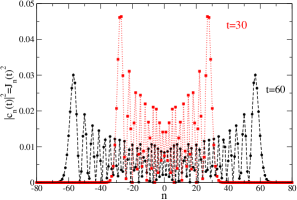
Figure 1: Probability to find the particle at site $n$ if it was localized in the state $|0\rangle$ at $t=0$ for two different times: t=30, squares on the dotted line; t=60, circles on the dashed line.

We have connected the discrete points at integer $n$ by a dotted line for $t=30$ and a dashed line for $t=60$. The result is drastically different from the broadening of a wave packet in the continuum. The dominant peaks indicate that the particle has a high probability to move with the maximum velocity in both directions. This can be understood using the probability distribution of the velocities in Eq. (45). For $|\phi\rangle=|0\rangle$ one has $|\langle k_{i}(v)|\phi\rangle|^{2}=1/2\pi$ leading

$$p_{\rm vel}(v)=\frac{1}{\pi}\frac{1}{\sqrt{1-v^{2}}}~{}.$$ (54)

The divergence of this function when approaching $\pm v_{\rm max}=\pm 1$ is responsible for the large weight near $n\approx\pm t$ in Fig. 1. The approach of the discrete probability density $|c_{n}(t)|^{2}$ to the continuous distribution $p_{\rm vel}(n/t)/t$ one would expect from Eq. (46) is obviously not a smooth one . weaklimit A simple averaging procedure better shows the importance of $p_{\rm vel}(n/t)/t$ for large enough $t$. We define

$$p_{\rm av}(n,t;n_{0})=\frac{1}{2n_{0}+1}\sum_{j=-n_{0}}^{n_{0}}|c_{n+j}(t)|^{2}~{}.$$ (55)

In Fig. 2 the continuous $p_{\rm vel}(n/t)/t$ is compared to the discrete averaged probability $p_{\rm av}(n,t;n_{0})$ for $t=60$ and $n_{0}=3$.

Figure 2: Averaged probability distribution $p_{\rm av}(n,t;n_{0})$ for $t=60$ and $n_{0}=3$ for the initial state $|0\rangle$. The dashed line shows $p_{\rm vel}(n/t)/t$.

To further elucidate the rather well defined edges of the packet in Fig. 1 at $n\approx\pm t$ we show the probability $|c_{n}(t)|^{2}$ for $n=30$ and $n=60$ as a function of time in Fig. 3.

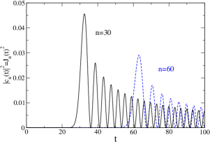
Figure 3: Probability to find the particle at two different sites as a function of time time $t$, if it was localized in the state $|0\rangle$ at $t=0$: $n=30$ (full line) and $n=60$ (dashed line).

The short time behaviour of $g_{n}(t)$ is discussed in the appendix (see Eq. (74)). This shows that $|c_{n}(t)|^{2}=J_{n}^{2}(t)$, is strongly suppressed for times $t$ small compared to $n$. Therefore the information that the particle was located at the origin at time $t=0$ arrives at site $n$ not before the time determined by $tv_{\rm max}=an$, which for $v_{\rm max}=1$ and $a=1$ is given by $t=n$. This is similar to the spread of information in spin systems on a lattice with finite range interactions. LiebRobinson ; Everts

For times $t\gg n$ the probability $|c_{n}(t)|^{2}=J_{n}^{2}(t)$ decays like $1/t$ in an oscillatory manner

$$J_{n}^{2}(t) \to \frac{2}{\pi t}\cos^{2}(t-\pi/4),~{}{\rm for}~{}n~{}~{}{\rm even}$$ (56)

$$\to \frac{2}{\pi t}\sin^{2}(t-\pi/4),~{}{\rm for}~{}n~{}~{}{\rm odd}~{}.$$ (57)

This follows from the large time behaviour of the Bessel functions of integer order discussed in the appendix. It describes the oscillatory behaviour of $|c_{n}(t)|^{2}$ very close to the origin in Fig. 1. For $t=n_{t}\pi$ with $n_{t}$ integer these small $n$ oscillations are suppressed and $|c_{n}(t)|^{2}\to 1/(\pi t)=p_{\rm vel}(0)/t$ for $n/t\to 0$, with $p_{\rm vel}$ presented in Eq.(54).

Next we show results where the initial state is Gaussian centered at the origin

$$c_{n}=\frac{1}{\sqrt{S}}e^{-n^{2}/(4d^{2})}~{},~{}~{}~{}S=\sum_{n}e^{-n^{2}/(2d^{2})}$$ (58)

where $d$ determines the width of the discrete Gaussian distribution $c_{n}^{2}$. The numerical evaluation of the corresponding sums shows that for increasing $d$ the width of the Gaussian wave packet on the lattice quickly approaches the continuum value $\Delta x=d$. Already for $d=1$ the deviation is extremely small. The expectation value $\langle\hat{v}^{2}\rangle$ can be calculated analytically. Using $n^{2}+(n+2)^{2}=2(n+1)^{2}+2$ in Eq. (39) yields

$$\langle\hat{v}^{2}\rangle=(1-e^{-2\tilde{d}^{2}})/2~{},$$ (59)

with $\tilde{d}=1/(2d)$. The convergence to the continuum value $\Delta v=\tilde{d}$ with increasing $d$ is slower than the approach of $\Delta x$ to $d$.

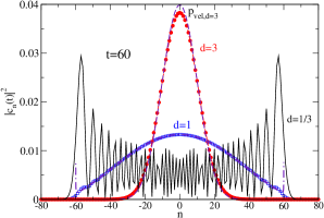
Figure 4: Probability to find the particle at site $n$ at time $t=60$ if the initial state was a Gaussian wave packet centered around the origin: $d=1/3$ (full line), $d=1.0$ (squares) and $d=3$ (full circles). Also shown is $p_{\rm vel}(n/60)/60$ for $d=1$ (dashed-dotted line) and $d=3$ (dashed line) with $|n|<60$ treated as a continuous variable.

In Fig. 4 we show the time dependent probability $|c_{n}(t)|^{2}$ as function of $n$ for $t=60$ and three different values of $d$. In contrast to Fig. 1 only the connecting curves of the values at integer $n$ are shown for $d=1/3$. This probability distribution differs little from the $t=60$ curve in Fig. 1. The $d=3$ result looks qualitatively similar to the broadening of a Gaussian wave packet on the continuum. The $d=1$ curve shows intermediate behaviour discussed below.

It is again useful to consider the corresponding $p_{\rm vel}(v)$. This requires to calculate $|\langle k|\phi\rangle|^{2}$, using Eq. (9). For large values of $d$ replacing the $n$-sum by an integral is a good approximation. This Gaussian integral leads to

$$|\langle k|\phi\rangle|^{2}_{\rm appr}=\left(\frac{2d^{2}}{\pi}\right)^{1/2}e^{-2d^{2}k^{2}}~{}.$$ (60)

Obviously one has lost the $2\pi/a$ periodicity of $|\langle k|\phi\rangle|^{2}$, where in this section we have put $a=1$. This is a minor problem if $|\langle k|\phi\rangle|^{2}_{\rm appr}$ differs from zero in a range smaller than $2\pi$.

Equation (43) allows to understand the crossover from the result for $|\phi\rangle=|0\rangle$ to the continuum like curve for $d=3$ in Fig. 4. For $v\to\pm 1$ the roots $k_{i}(v)$ approach the value $\pm\pi/2$. Therefore the value of $|\langle k=\pm\pi/2|\phi\rangle|^{2}$ is a measure for the suppression of the square root singularities of $p_{\rm vel}(v)$. They are almost completely suppressed for $d=3$, definitely present for $d=1/3$, and $d=1$ is an intermediate case. In Fig. 4 also $p_{\rm vel}(n/t)/t$ is shown for $d=1$ and $d=3$, treating $n$ as a continuous variable. For $d=1$ this provides an excellent approximation except for $|n|$ approaching $60$. For $d=3$ the deviations for small values of $n$ are larger, as $\Delta x/\Delta v$ is larger.

IV.2 Wave packets with finite average velocity

In order for the wave packet to have a finite average velocity $\langle\hat{v}\rangle$ the initial state has to have at least one pair of neighbouring sites with nonvanishing coefficients $c_{n}$, with a least one of them being a complex number. More generally we consider two-sites states

$$|\phi\rangle_{m}^{(k_{0})}=\frac{1}{\sqrt{2}}\left(|0\rangle+e^{imk_{0}}|m\rangle\right)$$ (61)

with $m\neq 0$.

Numerical results for $|c_{n}(t)|^{2}$ for $m=1$ are shown in Fig. 5. For the finite velocity case $k_{0}=1.0$ the probability distribution shows a clear asymmetry with respect to the origin. As for the single site initial state $p_{\rm vel}(v)$ for the two site states can easily be calculated. With

$$|\langle k|\phi\rangle_{m}^{(k_{0})}|^{2}=\frac{1}{2\pi}\left[1+\cos(m(k-k_{0}))\right]$$ (62)

one obtains using Eq. (45) for $m=1$

$$p_{\rm vel}(v)=\frac{1+v\sin k_{0}}{\pi\sqrt{1-v^{2}}}~{}.$$ (63)

For $k_{0}=\pm\pi/2$ the singularity at the lower (upper) edge of the distribution is suppressed completely. Fig. 5 also shows $p_{\rm vel}(n/t)/t$ for $k_{0}=1.0$.

Figure 5: Probability to find the particle at site $n$ at time $t$ if it was localized at the $m=1$ state in Eq. (61) at $t=0$ for two different values of $k_{0}$: $k_{0}=0$ (full line), $k_{0}=1$ (dotted line). The dashed line shows $p_{\rm vel}(n/t)/t$ for $p_{\rm vel}$ presented in Eq. (63) for $k_{0}=1.0$.

The probability distribution $p_{\rm vel}$ for $m=2$ is given by

$$p_{\rm vel}(v)=\frac{1}{\pi\sqrt{1-v^{2}}}\left[1+\cos(2k_{0})-2\cos(2k_{0})v^{2}\right]~{}.$$ (64)

For $k_{0}=0$ it reduces to $p_{\rm vel}(v)=2\sqrt{1-v^{2}}/\pi$, i.e. both singularities are suppressed as shown in Fig. 6. This example would also have fitted to section IV.A as the coefficients $c_{n}$ are real and $\langle v\rangle=0$.

Figure 6: Probability to find the particle at site $n$ at time $t=60$ for the $m=2,k_{0}=0$ initial state in Eq. (61) (circles). The squares show $p_{\rm av}(n,t;3)$ and the dashed curve $p_{\rm vel}(n/t)/t$.

Next we discuss boosted Gaussian initials state as in Eq. (47)

$$c^{(k_{0})}_{n}=e^{ik_{0}n}\frac{e^{-n^{2}/(4d^{2})}}{\sqrt{S}}~{}.$$ (65)

The expectation value $\langle\hat{v}^{2}\rangle^{(k_{0})}$ can again be calculated analytically using $n^{2}+(n+2)^{2}=2(n+1)^{2}+2$ in Eq. (39)

$$\langle\hat{v}^{2}\rangle^{(k_{0})}=(1-\cos 2k_{0}e^{-2\tilde{d}^{2}})/2.$$ (66)

For $d$ larger than the lattice constant it is a good approximation to replace the summation in Eq. (38) by an integration. Using $n^{2}+(n+1)^{2}=2(n+1/2)^{2}+1/2$ one obtains

$$\langle\hat{v}\rangle^{(k_{0})}\approx\sin k_{0}e^{-\tilde{d}^{2}/2},~{}~{}$$ (67)

The velocity uncertainty follows as

$$(\Delta v)^{(k_{0})}\approx\sqrt{(1+e^{-\tilde{d}^{2}}\cos 2k_{0})(1-e^{-\tilde{d}^{2}})/2}~{},$$ (68)

which explicitely shows the $k_{0}$ dependence. For large $d$ this uncertainty reaches the continuum value $\tilde{d}=1/(2d)$ for $k_{0}=0$. For $k_{0}=\pi/2$ it is proportional to $\tilde{d}^{2}$, i.e. the uncertainty product $\Delta x\Delta v$ vanishes like $1/d$. This implies that also for very broad wave packets the deviations from the Heisenberg uncertainty product can be large when the average velocity approaches the maximum velocity on the lattice as shown in Fig. 7

Figure 7: Uncertainty product $\Delta x\Delta v$ as a function of $k_{0}$ for different values of $d$: $d=1/3$ (dotted line), $d=1$ (dashed-dotted line), $d=3$ (dashed line), $d=30$ (full line).

For symmetry reasons it is sufficient to consider positive values of $k_{0}$ in the first Brillouin zone. Due to the properties of the functions $g_{n}(t)$ mentioned after Eq. (23) the probabilities $|c_{n}(t)|^{2}$ are identical for $k_{0}$ and $\pi-k_{0}$. Therefore the largest value we consider is $k_{0}=\pi/2$.

The corresponding amplitudes $\langle k|\phi\rangle$ follow from Eq. (9) by a shift of the $k$-value.

$$\langle k|\phi\rangle_{k_{0}}=\langle k-k_{0}|\phi\rangle_{k_{0}=0}~{}.$$ (69)

For $k_{0}>0$ this leads to $|\langle-\pi/2|\phi\rangle_{k_{0}}|^{2}<|\langle\pi/2|\phi\rangle_{k_{0}}|^{2}$. Therefore the singularity of $p_{\rm vel}(v)$ at $v=-1$ is stronger suppressed than the one at $v=1$, like in Eq. (61) for the two-site example.

In Fig. 8 we show results for $k_{0}=\pi/4,t=60$ and the same three values of $d$ as in Fig. 4. The average velocities are $0.141,0.604$ and $0.676$ for $d=1/3,1$ and $3$. Except for a slight asymmetry the $d=3$ curve again looks similar to the continuum case.

Figure 8: Probability to find the particle at site $n$ at time $t=60$ for the complex Gaussian initial state with $k_{0}=\pi/4$ in Eq. (65): $d=1/3$ (full line), $d=1.0$ (dashed dotted line) and $d=3$ (full circles). Also shown for $d=3$ is the corresponding $p_{\rm vel}(n/60)/60$ (dashed line).

In Fig. 9 the exact results for $d=1$ are compared to the corresponding $p_{\rm vel}(n/60)/60$.

Figure 9: Probability to find the particle at site $n$ at time $t=60$ for the complex Gaussian initial state with $d=1$ and $k_{0}=\pi/4$ in Eq. (65): exact results (full circles) and the corresponding $p_{\rm vel}(n/60)/60$ (dashed line).

The value of $|c_{n}(t)|^{2}$ for $n=60$ as a function of time is shown in Fig. 10 for the complex Gaussian initial state with $k_{0}=\pi/4$ for the same values of $d$ as in Fig. 8.

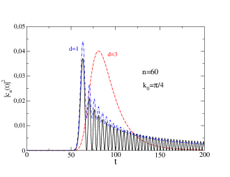
Figure 10: Probability to find the particle at site $n=60$ as a function of time $t$, if it was in a complex Gaussian initial state of width $d$ and $k_{0}=\pi/4$: $d=1/3$ (full line), $d=1$ (dashed-dotted line) and $d=3$ (dashed line).

For all three values of $d$ the probability to find the particle at site $n=60$ for times smaller than $t=n/v_{\rm max}=60$ is very small.

We finally consider the case $k_{0}=\pi/2$, which is very special. For all positive values of $k_{0}$ smaller than $\pi/2$ it is possible to suppress the square root singularity at $v=1$ in $p_{\rm vel}(v)$ by choosing $d$ large enough. For $k_{0}=\pi/2$ the maximum of $|\langle k|\phi\rangle|^{2}$ is right at $k=\pi/2$. The average velocity takes the largest value. For $d\to\infty$ it reaches the value $v_{\rm max}=1$. For $d=3$ and $k_{0}=\pi/2$ the average velocity is $\langle\hat{v}\rangle=0.986$.

As $\epsilon_{\pi/2+\tilde{k}}=\sin\tilde{k}$ the energy dispersion is approximately linear around $k_{0}=\pi/2$ and $v_{\pi/2+\tilde{k}}\approx 1-\tilde{k}^{2}/2$. It is shown in Fig. 11 that the deviations from a strictly linear energy dispersion become important for large enough times.

Figure 11: Probability distribution $|c_{n}(t)|^{2}$ for $k_{0}=\pi/2$ and $d=3$ as a function of $n-t$ for different times : $t=0$ circles (full line), $t=100$ squares (dashed line) and $t=500$ diamonds (dashed-dotted line). For $t=500$ also $p_{\rm vel}(n/t)/t$ is shown (dashed line).

As the results are shown as a function of $n-t$ there is a visible shift of the distribution to smaller values for increasing time. The oscillatory behaviour clearly visible for $n-t<15$ for the $t=500$ distribution is an effect that does not occur in the continuum case for a strictly linear dispersion. It is smoothed out in the velocity distribution function, for $d\gg 1$ and $v$ approaching $1$ given by

$$p_{\rm vel}(v)\approx 2\sqrt{\frac{2d^{2}}{\pi}}\frac{\exp{[-4d^{2}(1-v)]}}{\sqrt{1-v^{2}}}~{}.$$ (70)

It is also shown in Fig. 11.

V Summary

Several aspects of the propagation of wave packets in a one-dimensional tight-binding chain with nearest neighbour hopping were presented. For an initial state localized at a single site a totally different time dependence shows up compared to the well known behaviour of a narrow Gaussian wave packet in the continuum. An important quantity for the understanding of the large probabilities to find the particle at time $t$ near positions $\pm v_{\rm max}t$ is the divergence of the probability distribution $p_{\rm vel}(v)$ at the values $\pm v_{\rm max}$. For strongly localized initial states the probabilities $|c_{n}(t)|^{2}$ to find the particle at site $n$ is strongly varying with $n$. Introducing an appropriate local averaging procedure one can obtain smoother functions of $n$. In the long-time limit these functions approach $p_{\rm vel}(n/t)/t$.

In order for the wave packet to have a finite average velocity at least a two-site initial state involving a complex amplitude is necessary. For an initial state with symmetric nearest neighbour site occupancies this leads at finite times to an asymmetry in the site probability distribution. This can easily be understood by again analytically calculating $p_{\rm vel}$.

Gaussian initial states with zero and finite average velocity were studied in detail. Even for initial widths much larger than the lattice constant clear differences to the continuum case arise for average velocities close to $\pm v_{\rm max}$.

The generalization to higher dimensional lattices is straightforward. For a single site initial state in the origin of a square lattice with nearest neighbour hopping the probability to find the particle at position $n_{x},n_{y}$ is given by $J_{n_{x}}(t)^{2}J_{n_{y}}(t)^{2}$ if the hopping matrix elements in the $y$-direction are identical to the one in the $x$-direction.

VI Acknowledgements

The author would like to thank Gerhard Hegerfeldt, Reiner Kree, Salvatore Manmana and Volker Meden for a critical reading of the manuscript and useful comments.

Appendix A Bessel functions of integer order

In this appendix we present a simple new way to calculate $g_{n}(t)=\langle n|e^{-i\hat{H}t/\hbar}|0\rangle$ which directly shows that it is proportional to the Bessel function $J_{n}(\tilde{t})$.

The starting point is to write the time evolution operator $e^{-i\hat{H}t/\hbar}$ in product form using $\hat{H}=\epsilon_{01}(\hat{T}_{\pm a}+T^{\dagger}_{\pm a})$. As the translation operators $\hat{T}_{a}$ and $\hat{T}_{-a}$ commute one has using Eq. (49)

$$e^{-i\hat{H}t/\hbar}=e^{i\tilde{t}\hat{T}^{\dagger}_{\pm a}/2}e^{i\tilde{t}\hat{T}_{\pm a}/2}$$ (71)

with $\tilde{t}=-2\epsilon_{01}t/\hbar$. This allows a simple calculation of $g_{n}(t)$ without the use of the eigenstates of the Hamiltonian.

For $n\geq 0$ one obtains applying the second factor to the right and the first one to left

$$e^{i\tilde{t}\hat{T}_{\pm a}/2}|0\rangle = \sum_{l=0}^{\infty}\frac{(i\tilde{t}/2)^{l}}{l!}|\pm l\rangle$$

$$\langle\pm n|e^{i\tilde{t}\hat{T}^{\dagger}_{\pm a}/2} = \sum_{m=0}^{\infty}\langle\pm(n+m)|\frac{(i\tilde{t}/2)^{m}}{m!}~{}.$$ (72)

Taking the scalar product yields the power series

$$g_{\pm n}(t)=i^{n}\left(\frac{\tilde{t}}{2}\right)^{n}\sum_{m=0}^{\infty}\frac{(-\tilde{t}^{2}/4)^{m}}{(m+n)!m!}=i^{n}J_{n}(\tilde{t})~{}.$$ (73)

The power series for $J_{n}(x)$ is usually obtained by solving the Bessel differential equation by a power series ansatz. AS

Alternatively the power series for $g_{\pm n}(t)$ can be obtained by performing the $\tilde{k}$ integration in Eq. (23) after expanding $e^{i\tilde{t}\cos\tilde{k}}$ in the integrand.

The short time approximation for $g_{\pm n}(t)$ follows from Eq. (73) as

$$g_{\pm n}(t)=i^{n}\frac{(t/2)^{n}}{n!}\left(1-\frac{t^{2}/4}{n+1}+...\right)~{}.$$ (74)

The long time approximation for $J_{n}(t)$ can be obtained using the stationary phase method for the integral in Eq. (23). For fixed $n$ this yields AS

$$J_{n}(t)\to\sqrt{\frac{2}{\pi t}}\cos{\left(t-\frac{\pi}{4}-\frac{n\pi}{2}\right)}~{}.$$ (75)

A detailed discussion of $J_{n}(t)$ for large $n$ and $t\approx n$ can be found in reference 12.

References

- (1) R.P. Feynman, R.B. Leighton, M. Sands, The Feynman Lectures on Physics, Vol. 3, Chapter 12; Adison-Wesley, Reading Massachusetts (1965)
- (2) N.W. Ashcroft and N.D. Mermin, Solid State Physics, Chapter 11, Harcourt College Publishers, Fort Worth (1976)
- (3) E. Farhi and S. Gutmann, “ Quantum computation and decision trees”, Phys. Rev. A 58, 915-928 (1998)
- (4) E.H. Lieb and D. W. Robinson, “ The finite group velocity of quantum spin systems”, Commun. math. Phys. 28, 251-257 (1972)
- (5) M. Ganahl, E. Rabel, F.L. Essler, and H.G. Everts, “Observation of Complex Bound States in the Spin-1/2 Heisenberg XXZ Chain”, Phys. Rev. Lett. 108, 077206 (1-5) (2012)
- (6) K. Mita, Dispersion of non-Gaussian free particle wave packets, Am. J. Phys. 75, 950-953, (2007). This paper presents a list of some earlier papers published in Am. J. Phys. on wave packets in a one-dimensional continuum.
- (7) K. Schönhammer, “Canonically conjugate pairs and phase operators”, Phys. Rev. A66, 041101 (1-4) (2002)
- (8) O. Mülken and A. Blumen, “Spacetime structures and continuous time quantum walks”, Phys. Rev. E 71, 036128 (1-5) (2005). In this paper additional references are given.
- (9) E. Merzbacher, Quantum Mechanics 3rd edition (John Wiley and Sons, New York, 2000)
- (10) M. Abramowitz and I. Stegun, Handbook of Mathematical Functions , Dover Publications, New York (1965). The Bessel functions of integer order are presented in chapter 9. The integral representation has the number 9.1.21
- (11) There is only weak convergence of the probability distributions: N.Konno, “Limit theorem for continuous-time quantum walks”, Phys. Rev. E 72, 026133 (2005), A.D. Gottlieb, “Convergence of continuous-time quantum walks on the line” Phys. Rev. E 72, 047102 (2005)
- (12) F.W.J. Olver, “Some new asymptotic expansions for Bessel functions of large order”, Math. Proc. Camb. Philos. Soc. 48, 418-427 (1952)