Pégase.3: A code for modeling the UV-to-IR/submm spectral
and chemical evolution of galaxies with dust

A code computing consistently the evolution of stars, gas and dust, as well as the energy they radiate, is required to derive reliably the history of galaxies by fitting synthetic spectral energy distributions (SEDs) to multiwavelength observations. The new code Pégase.3 described in this paper extends to the far-infrared/submillimeter the ultraviolet-to-near-infrared modeling provided by previous versions of Pégase. It first computes the properties of single stellar populations at various metallicities. It then follows the evolution of the stellar light of a galaxy and the abundances of the main metals in the interstellar medium (ISM), assuming some scenario of mass assembly and star formation. It simultaneously calculates the masses of the various grain families, the optical depth of the galaxy and the attenuation of the SED through the diffuse ISM in spiral and spheroidal galaxies, using grids of radiative transfer precomputed with Monte Carlo simulations taking scattering into account. The code determines the mean radiation field and the temperature probability distribution of stochastically heated individual grains. It then sums up their spectra to yield the overall emission by dust in the diffuse ISM. The nebular emission of the galaxy is also computed, and a simple modeling of the effects of dust on the SED of star-forming regions is implemented.

The main outputs are ultraviolet-to-submillimeter SEDs of galaxies from their birth up to $20\mathclose{}\,\mathopen{}\mathrm{Gyr}$, colors, masses of galactic components, ISM abundances of metallic elements and dust species, supernova rates. The temperatures and spectra of individual grains are also available. The paper discusses several of these outputs for a scenario representative of Milky Way-like spirals.

Pégase.3 is fully documented and its Fortran 95 source files are public. The code should be especially useful for cosmological simulations and to interpret future mid- and far-infrared data, whether obtained by JWST, LSST, Euclid or e-ELT.

1 Introduction

Multiwavelength observations of galaxies from the far-ultraviolet to the far-infrared and submillimeter – the spectral domain in which ordinary galaxies emit almost all their light – should allow reconstruction of their history and that of their stars, gas and dust. Many deep surveys have already been carried out to derive the evolution on cosmological timescales of the stellar mass for a large number of objects of various types. In particular, determining the history of mass assembly of galaxies might help to assess the respective contributions of hierarchical merging and early dissipative collapse to the formation of galaxies, and, ultimately, to settle the long-standing astrophysical debate over which was the dominant process.

To this purpose, several teams have built codes to synthesize panchromatic spectral energy distributions (SEDs), fit them to observations of galaxies, whether individual or in surveys, and derive their ages, masses, star formation rates, chemical compositions, and opacities (e.g., the code Beagle by Chevallard & Charlot, 2016, to name a recent one). A first difficulty is to jointly follow the evolution of gas and dust in the interstellar medium (ISM) and that of the stellar populations that form from the latter and enrich it. Another difficulty is to model properly the attenuation and scattering by dust grains of the light emitted by stars in the ultraviolet (UV) and the optical, as well as the re-emission at longer wavelengths of the energy these grains absorbed. As discovered by IRAS and confirmed by ISO, Spitzer and Herschel, this process dominates at all wavelengths from the mid- to the far-infrared (IR). It is therefore essential to model it consistently to put reliable constraints on the evolution of galaxies using synthetic SEDs. This is the main objective of the code Pégase.3 described in this paper.

A large variety of spectral synthesis codes already exist (for review papers, see Walcher et al., 2011 and Conroy, 2013). Some, such as Starburst99 (Leitherer et al., 1999, 2014) and codes based on it (e.g., Steidel et al., 2016), focus on the modeling of young stellar populations ($\mathord{\la}\,100\mathclose{}\,\mathopen{}\mathrm{Myr}$) and their nebular environment; they are typically applied to the analysis of the continuum and of emission lines at UV–optical wavelengths. The code of Dopita et al. (2005), which couples Starburst99 and Mappings, also computes the infrared emission produced by the dust cloud surrounding a star cluster. Although these codes are very appropriate to study current or recent starbursts, they are not suitable for evolved galaxies.

The first code following the evolution of the stellar light emitted by a galaxy on cosmological timescales was built by Tinsley (1972). It computed the mass and overall metallicity of the interstellar medium as a function of time, and implemented laws relating the star formation rate to the gas content. This code produced however only optical colors.

The spectral evolution code of Bruzual (1983) was a significant improvement, not only with regard to the photometric evolution codes of Tinsley (1972) and Rocca-Volmerange et al. (1981), but also when compared to then-existing spectral population synthesis codes (e.g., Alloin et al., 1971), which simply fitted the SEDs of galaxies with linear combinations of observed SEDs of stars or star clusters.

The extension to the near-infrared was a difficult challenge, because it required to follow the rapid stellar phases (the late asymptotic giant branch, mainly) dominating these wavelengths. This problem was solved by Charlot & Bruzual (1991) through the method of isochrones, also used since the first version of code Pégase (Fioc & Rocca-Volmerange, 1997). Another solution, based on the fuel consumption theorem (see Renzini & Buzzoni, 1983, for instance), was implemented by Maraston (2005).

Many other developments occurred meanwhile. To cite a few, Guiderdoni & Rocca-Volmerange (1987) modeled the metallicity-dependent attenuation of a galaxy SED by dust grains distributed in a slab; Worthey (1994) considered the effect of non-solar abundance ratios of metals on the spectrum of a single stellar population; Fioc & Rocca-Volmerange (1999b; Pégase.2) computed consistently the metallicity and the spectral evolution, from the UV to the near-IR, using metallicity-dependent stellar spectra, evolutionary tracks and yields; Devriendt et al. (1999) developed the code Stardust and used it in Galics (Hatton et al., 2003; Cousin et al., 2015) to run semi-analytic simulations of galaxy formation; Boissier & Prantzos (1999) modeled in detail the radial dependency of the spectrochemical evolution of spiral galaxies; Eldridge et al. (2008, 2017) explored the effects of binaries.

To extend spectral evolution codes to longer wavelengths, it was necessary to model properly dust grains and their effects in attenuation and emission. Fits of the Milky Way’s extinction curve by Mathis et al. (1977) initially suggested that dust was a mixture of silicate and graphite grains with sizes larger than $0.005\mathclose{}\,\mathopen{}\mathrm{\muup m}$, but the analysis of the mid-IR features observed in reflection nebulae led Sellgren (1984) to propose that these were caused by much smaller, stochastically heated particles. Léger & Puget (1984) subsequently identified these particles as polycyclic aromatic hydrocarbons (PAHs); these molecules are now commonly included in models of dust composition and grain size distribution (e.g., Zubko et al., 2004; Weingartner & Draine, 2001). The evolution of the two main families of grains, namely carbonaceous and silicate ones, was modeled by Dwek (1998), taking into account their formation, destruction and accretion on preexisting grains.

Several galaxy evolution models compute the attenuation by dust of the UV–optical light using global effective attenuation curves such as the ones proposed by Calzetti et al. (1994; recently updated by Battisti et al., 2016), Charlot & Fall (2000) or Conroy (2010). Effective attenuation curves were also used by Lo Faro et al. (2017) to fit the UV–IR SED of galaxies with Cigale (Buat et al., 2014), a code enforcing the energy balance between dust absorption and dust emission.

The energy balance argument is also invoked in the codes Stardust (Devriendt et al., 1999) and Magphys (da Cunha et al., 2008) to estimate the integrated emission by dust; this emission is then apportioned among predefined SEDs corresponding to PAHs, small and big graphite and silicate grains with temperatures fixed beforehand. These codes do not, however, compute the temperature distribution of individual grains stochastically heated by the radiation field. Neither do they follow the evolution of the dust content in the ISM.

True radiative transfer codes are required to determine the attenuation and emission by dust more reliably. Several techniques have been developed to this purpose: Grasil (Granato et al., 2000; Lacey et al., 2008), for instance, is based on Monte Carlo simulations; on the other hand, the recent modeling by Cassarà et al. (2015) uses the ray-tracing method.

All codes have to make compromises between efficiency, completeness, accuracy and consistency. Some of the codes listed above are more physical than Pégase.3 in some respects, but are so numerically intensive that they are restricted in practice to the study of single objects or specific categories of galaxies. Others are more phenomenological and, while they may be very handy to analyze large surveys, give little insight on the evolution of galaxies because the various components, in particular stars and dust, are modeled separately; they have therefore little predicting power.

Pégase.3 aims to reconcile efficiency, consistency and realistic modeling in a general-purpose code, appropriate for studies of the chemical and far-UV-to-submillimeter (submm) spectral evolution of Hubble sequence galaxies from their formation up to now. The variety of the inputs used to compute galaxy models, the wealth of its outputs and its modular structure should make it particularly suited to cosmological simulations. Its source files, written in Fortran 95, are moreover entirely public and may be freely adapted by the user. For technical details, see the documentation (Fioc & Rocca-Volmerange, 2019).

Section 2 of this paper first describes the system considered by Pégase.3, and how the code consistently computes the spectral evolution of a galaxy’s stellar component and the chemical evolution of its interstellar medium (ISM) for a given scenario of mass assembly and star formation. We detail in particular the inputs used to model single stellar populations. Section 3 is devoted to the characteristics of grains – their optical properties and size distribution – and to their evolution in the ISM. Section 4 focuses on the radiative transfer of the stellar light through the dusty diffuse ISM in spiral and spheroidal galaxies. The computation of dust emission, taking into account the stochastic heating of grains by the radiation field, is treated in Sect. 5. The modeling of nebular emission and of star-forming clouds is dealt with in Sect. 6. In Sect. 7, we highlight some outputs of Pégase.3, taking as an example a scenario representative of Milky Way-like galaxies. Finally, Sect. 8 concludes on the strengths and limitations of the code, its existing and potential applications, and lists some intended improvements.

2 Emission of stellar populations and chemical evolution

2.1 The system

The system considered in the code is formed of the galaxy proper, of reservoirs furnishing the gas falling onto the galaxy (infall), and of interstellar matter ejected by the galaxy into the intergalactic medium (outflow): so, the galaxy is modeled as an open box, but the total mass of the system, $M_{\mathrm{sys}}$, is constant. The evolution of the galaxy from its initial state is determined by a scenario providing, among others, the parameters from which the star formation, infall and outflow rates are computed as a function of time. All the parameters defining a scenario are described in detail in the code’s documentation (Fioc & Rocca-Volmerange, 2019); they are organized in trees for convenience.

The code follows the evolution of the interstellar medium (ISM; both gas and dust), of the stars it contains and of the mass locked in compact stellar remnants (black holes and neutron stars). Two regions are distinguished in the ISM: the diffuse medium and star-forming clouds (see Silva et al., 1998 and Charlot & Fall, 2000 for other instances of this distinction).

2.2 Modeling of single stellar populations

2.2.1 Overview

The basic unit of a galaxy evolution model is a single stellar population (SSP), that is, a set of stars, with the same initial chemical composition, created by an instantaneous star-forming event. The monochromatic luminosity (or “spectral flux”, in radiometric terminology; denoted by $L_{\lambda}$ hereafter) per unit wavelength of an SSP with an initial chemical composition $\{\chi_{0}\}\coloneqq\{\chi_{0}(\mathrm{H}),\chi_{0}(\mathrm{He}),\ldots\}$ is, per unit initial mass of the SSP,

$$L_{\lambda}^{\textsc{ssp}}(t,\{\chi_{0}\})=\int L_{\lambda}^{\mathrm{star}}(m,t,\{\chi_{0}\})\mathclose{}\,\mathopen{}\phi(m)\mathclose{}\,\mathopen{}\mathrm{d}(\ln m)$$ (1)

at age $t$ and wavelength $\lambda$, where $L_{\lambda}^{\mathrm{star}}(m,t,\{\chi_{0}\})$ is the monochromatic luminosity at this age of a star with an initial mass $m$ and initial composition $\{\chi_{0}\}$, and $\phi$ is the initial mass function (IMF): $\phi(m)\mathclose{}\,\mathopen{}\mathrm{d}(\ln m)$ is the number of stars, per unit initial mass of the SSP, born with a mass in the interval $[m,m+\mathrm{d}m\mathclose{[}$; this function is normalized, that is, $\int m\mathclose{}\,\mathopen{}\phi(m)\mathclose{}\,\mathopen{}\mathrm{d}(\ln m)=1$. A large number of IMFs are available in the code.

The luminosity $L_{\lambda}^{\mathrm{star}}$ is computed as

$$L_{\lambda}^{\mathrm{star}}(m,t,\{\chi_{0}\})=\mathcal{L}_{\mathrm{star}}(m,t,\{\chi_{0}\})\mathclose{}\,\mathopen{}\ell_{\lambda}^{\mathrm{star}}(\{\chi_{\mathrm{surf}}\},T_{\mathrm{eff}},g)\,,$$ (2)

where $\mathcal{L}_{\mathrm{star}}$ is the bolometric luminosity (or “radiant flux”, in radiometric terminology; all integrated luminosities are denoted by $\mathcal{L}$ hereafter) of the star, that is, the amplitude of the stellar spectrum, and the function $\lambda\mapsto\ell_{\lambda}^{\mathrm{star}}$ is the shape of this spectrum. This shape depends mainly on three quantities: the surface composition $\{\chi_{\mathrm{surf}}\}$ of the star, its effective temperature $T_{\mathrm{eff}}$ and its surface gravity $g$. Because of limitations in the input data, we use a single number, the initial metallicity $Z$ of a star – its mass fraction of metals at birth –, as a substitute for both the initial and surface sets of abundances, $\{\chi_{0}\}$ and $\{\chi_{\mathrm{surf}}\}$. The quantities $\mathcal{L}_{\mathrm{star}}$, $T_{\mathrm{eff}}$ and $g$ are given by stellar evolutionary tracks as a function of $m$, $t$ and $Z$. The shape is interpolated as a function of $Z$, $T_{\mathrm{eff}}$ and $g$ from the elements of a metallicity-dependent library of stellar spectra. To compute $L_{\lambda}^{\textsc{ssp}}$ from Eq. (1), we derive from the evolutionary tracks the isochrone of an SSP at age $t$, that is, the locus of all the stars in the $(\mathcal{L}_{\mathrm{star}},T_{\mathrm{eff}},g)$ ($\mathord{\approx}\,$Hertzsprung & Russell; HR) diagram.

2.2.2 Stellar evolutionary tracks

Stellar evolutionary tracks provide the evolution of the bolometric luminosity, effective temperature and surface gravity as a function of age for a range of initial masses. They should ideally be available for all the initial compositions (or initial metallicities, at least) occurring during the evolution of a galaxy, cover all the masses in the IMF and all the evolutionary phases of a star.

The default set is based on the classical “Padova” tracks (Bressan et al., 1993; Fagotto et al., 1994a, b, c; Girardi et al., 1996), from $Z=0.0001$ up to $Z=0.1$. For stars undergoing the helium flash, the mass loss along the red (or “first”) giant branch (RGB) and early asymptotic giant branch (AGB) phases is modeled with the law of Reimers (1975) and multiplied by an efficiency $\eta$ (Renzini, 1981); we take $\eta=0.4$, as recommended by the authors of the Padova tracks. Pseudo-tracks are then computed for the thermally pulsing AGB phase, using the equations proposed by Groenewegen & de Jong (1993) with $\eta=4$ (van den Hoek & Groenewegen, 1997). Hydrogen-burning post-AGB and CO white dwarf tracks are derived from Blöcker (1995), Schönberner (1983), Koester & Schönberner (1986) and Paczyński (1971). For low-mass stars becoming helium white dwarfs, the Althaus & Benvenuto (1997) models are used, while the nearly unevolving positions of low-mass stars ($m<0.6\mathclose{}\,\mathopen{}M_{\odot}$) in the HR diagram come from Chabrier & Baraffe (1997).

2.2.3 Stellar yields

Stars eject matter in the interstellar medium (ISM) through stellar winds and when they explode as supernovae. When the code computes the chemical evolution of a galaxy, it is assumed that the ejection of matter by a star happens only at the end of its life: this approximation is justified by the short life of high-mass stars, compared to the age of a galaxy, and by the late onset of intense winds in low-mass stars. The recycling of matter in galaxies modeled by Pégase is therefore not instantaneous.

For low-mass stars ($m/M_{\odot}\leqslant 5$ or $6$ in Padova tracks), stellar winds occur mainly during the RGB and AGB phases; the final remnant is a white dwarf. We used the yields in tables A7 to A12 of Marigo (2001), given for a mixing-length parameter $\alpha=1.68$ at $Z\in\{0.004,0.008,0.019\}$, and extrapolated them at the metallicities of the Padova tracks.

Higher-mass stars undergo strong stellar winds during their whole life and usually end as core-collapse supernovae (i.e., of type II, Ib or Ic); the final remnant is a neutron star or a stellar black hole, depending on the progenitor’s mass. For these stars, the code’s default yields are from Portinari et al. (1998). The choice of the supernova yields, with no winds, from model B of Woosley & Weaver (1995) is also possible, but we had to extrapolate them above an initial mass of $40\mathclose{}\,\mathopen{}M_{\odot}$ and below $11\mathclose{}\,\mathopen{}M_{\odot}$. Files containing all the computed yields are available with the code.

Although more-recent yields have been published (see the review by Nomoto et al., 2013, in particular for high-mass stars, and, for low-mass stars, Karakas, 2010), the yields of Marigo (2001) and Portinari et al. (1998) have the advantage that they were computed consistently with the classical Padova tracks. Another merit of the latter is that they distinguish the wind and core-collapse phases, which is needed when dust ejecta by stars are computed using the sophisticated model described in Sect. 3.2.

According to the favorite model, type Ia supernovae occur in close binaries where the primary star becomes a CO white dwarf ending in a thermonuclear explosion. We use the prescriptions of Greggio & Renzini (1983) and Matteucci & Greggio (1986) to model the number of close binaries and the rate of type Ia supernovae. The ejecta produced by the exploding CO white dwarf are those of model W7 of Thielemann et al. (1986). As an example, we show in Fig. 1 the ejection rate of various elements by a single stellar population with a metallicity $Z=0.02$, and the ejecta cumulated since the birth of the SSP.

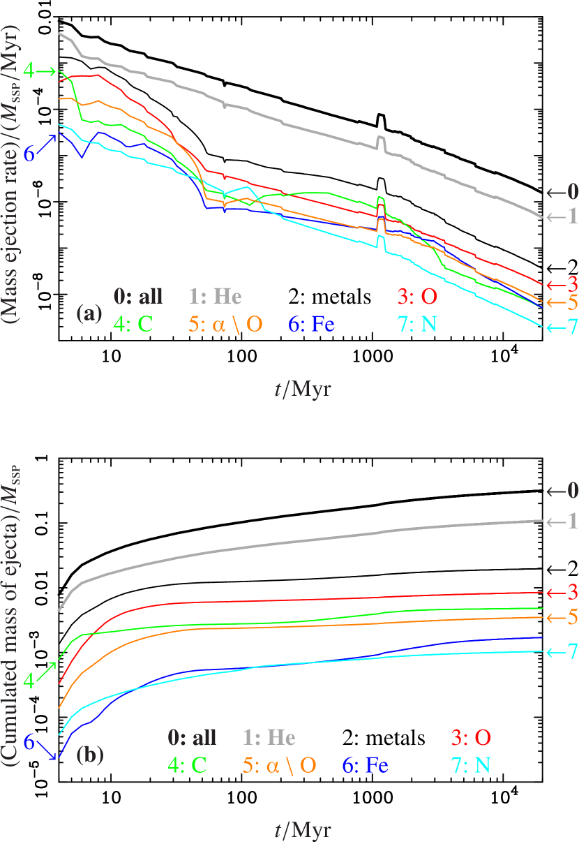
Figure 1: Ejecta produced at or until age $t$ by a single stellar population with an initial metallicity $Z=0.02$ (in mass fraction), the Kroupa et al. (1993) IMF and Portinari et al. (1998) yields for massive stars; the fraction of close binary stellar systems is $0.05$.(a) Ejection rate in mass of ejecta per unit time per unit initial mass of the SSP: “all” denotes the sum on all ejected elements; “metals”, the sum on all metals; “$\alphaup\setminus\mathrm{O}$”, the sum on the main $\alphaup$-elements except oxygen (i.e., Ne, Mg, Si, S and Ca). The bump after $1\mathclose{}\,\mathopen{}\mathrm{Gyr}$ is due to RGB stars undergoing the helium flash. (b) Cumulated mass of ejecta per unit initial mass of the SSP.

2.2.4 Libraries of stellar spectra

The main aim of Pégase.3 is to model the effects of dust on the spectral energy distribution of a galaxy. To do this, the library of stellar spectra must have a large and continuous wavelength coverage, from the far-UV to the near-IR (at least), but a high spectral resolution is not required. The library of stellar spectra used in Pégase.3 is made of two blocks: BaSeL’s spectra for stars with an effective temperature $T_{\mathrm{eff}}<50\mkern 2.0mu000\mathclose{}\,\mathopen{}\mathrm{K}$; the spectra from Rauch (2003), rebinned to the wavelengths of BaSeL, for hotter stars (available only at $[\mathrm{Fe}/\mathrm{H}]\in\{-1,0\}$). The emission rate of Lyman continuum photons by stars is computed from these spectra.

The BaSeL library is based on theoretical spectra, from Kurucz (1979) mostly, corrected to fit in the near-UV–near-IR domain the observed colors of stars and star clusters with various metallicities. Two versions are implemented in the code: the default one, v2.2 (Lejeune et al., 1998), and v3.1 (Westera et al., 2002).

2.3 Star formation history, mass assembly and chemical evolution

The stellar content of a galaxy is composed of SSPs with various ages and metallicities. The unattenuated stellar monochromatic luminosity of a galaxy, at age $t$ and wavelength $\lambda$, is

$$L_{\lambda}^{\star,\,0}(t)=\int_{t^{\prime}=0}^{t}\psi(t-t^{\prime})\mathclose{}\,\mathopen{}L_{\lambda}^{\textsc{ssp}}(t^{\prime},Z[t-t^{\prime}])\mathclose{}\,\mathopen{}\mathrm{d}t^{\prime}\,\!,$$ (3)

where $\psi(t-t^{\prime})$ is the star formation rate (SFR) at time $t-t^{\prime}$, and $Z(t-t^{\prime})$ is the metallicity of the interstellar medium at that time.

In the code, the star formation rate is computed from the star formation law the user chose for the scenario. The parameters determining the infall rate of gas from the reservoirs onto the galaxy and the outflow rate of matter from the galaxy into the intergalactic medium – that is, the mass assembly history of the galaxy – are also set by the scenario. A large variety of scenarios may be built from the trees of parameters described in the code’s documentation. In particular, one or more instantaneous or extended, overlapping or consecutive episodes of star formation may occur, and the same holds for infall and outflow.

The first reason why, since Fioc (1997) and Rocca-Volmerange & Fioc (1999), open-box models are preferred in Pégase is that simpler, closed-box models predict the presence of a large proportion of low-metallicity stars, which is detected neither in spiral galaxies (Prantzos & Silk, 1998) – the “G-dwarf problem” – nor in ellipticals (Henry & Worthey, 1999) and would lead to bluer UV-to-near-IR galaxy SEDs and colors than what is observed. Closed-box models also fail to account for the age-metallicity relation in the Milky Way (see, e.g., Twarog, 1980; Tosi, 1988). Conversely, Boissier & Prantzos (2000) and Tantalo et al. (1996) respectively modeled late-type and early-type galaxies satisfactorily with infall (see also Sommer-Larsen et al., 2003). As emphasized by Larson (1972) and Lynden-Bell (1975), it is unrealistic to postpone the beginning of star formation in a model until the complete assembly in the galaxy proper of all its gas.

As regards outflows of matter, whatever their cause (e.g., large-scale galactic winds driven by supernovae, as in Mathews & Baker, 1971), they are required to explain the enrichment of the intergalactic medium and are a possible explanation for the star formation quenching observed in early-type galaxies (Pozzetti et al., 2010; Ciesla et al., 2016). For a recent review of the many theoretical and observational motivations to consider exchanges of matter between galaxies and their circumgalactic environment, see Tumlinson et al. (2017).

The chemical evolution of a galaxy is likewise determined by the scenario. For the evolution of the mass of metals, for instance,

$$\begin{split}\!\frac{\mathrm{d}(M_{\textsc{ism}}\mathclose{}\,\mathopen{}Z_{\textsc{ism}})}{\mathrm{d}t}&=-(\psi\mathclose{}\,\mathopen{}Z_{\textsc{ism}})(t)\\ &\mathrel{\phantom{=}}\mathord{}\mskip-4.0mu plus -2.0mu minus -4.0mu+\sum_{j=1}^{n_{\mathrm{res}}}\dot{M}_{\mathrm{in},\,j}(t)\mathclose{}\,\mathopen{}Z_{\mathrm{in},\,j}-(\dot{M}_{\mathrm{out}}\mathclose{}\,\mathopen{}Z_{\textsc{ism}})(t)\\ &\mathrel{\phantom{=}}\mathord{}\mskip-4.0mu plus -2.0mu minus -4.0mu+\int_{t^{\prime}=0}^{t}\psi(t-t^{\prime})\mathclose{}\,\mathopen{}\dot{M}_{\mathrm{ej},\,Z}^{\textsc{ssp}}(t^{\prime},Z[t-t^{\prime}])\mathclose{}\,\mathopen{}\mathrm{d}t^{\prime}\,\!,\end{split}$$ (4)

where $M_{\textsc{ism}}$ and $Z_{\textsc{ism}}$ are the mass of matter and the metallicity in the ISM, $n_{\mathrm{res}}$ is the number of reservoirs, $\dot{M}_{\mathrm{in},\,j}$ and $Z_{\mathrm{in},\,j}$ are the infall rate from reservoir $j$ and its metallicity, $\dot{M}_{\mathrm{out}}$ is the outflow rate into the intergalactic medium, and $\dot{M}_{\mathrm{ej},\,Z}^{\textsc{ssp}}$ is the mass ejection rate of metals by an SSP into the ISM. The code computes in the same way the evolution of the ISM abundances of He, C, N, O, Ne, Mg, Si, S, Ca and Fe. These equations assume that stellar ejecta are instantaneously and homogeneously mixed with the ISM once in it, and that the composition of galactic outflows is the same as that of the ISM.

3 Properties of grains and dust evolution

3.1 Grain sizes and optical properties

Two families of dust grains are considered. The first family contains only one species, silicate grains. The other family, the carbonaceous grains, is subdivided in three species: graphites, neutral polycyclic aromatic hydrocarbons (PAHs) and ionized PAHs.

In the code, the weights of grain species within their family and the size distribution of grains in a given species are assumed to be constant. The following models of these properties are implemented: (1) the “bare_gr_s” model of Zubko et al. (2004) (by default); (2) model number $7$ in table 1 of Weingartner & Draine (2001), used in Li & Draine (2001); (3) the outdated model, without PAHs, of Mathis et al. (1977).

The global optical properties of dust species are computed as a function of wavelength from the size distributions and from the optical properties of individual grains given by Laor & Draine (1993), Draine & Lee (1984) and Li & Draine (2001). The extinction opacity in surface per unit mass (also called the “mass extinction coefficient”) of dust species $i$ at wavelength $\lambda$ is

$$\kappa_{i,\,\lambda}^{\mathrm{ext}}=\int_{a}\pi\mathclose{}\,\mathopen{}a^{2}\mathclose{}\,\mathopen{}\Bigl{(}Q_{i,\,\lambda}^{\mathrm{abs}}[a]+Q_{i,\,\lambda}^{\mathrm{sca}}[a]\Bigr{)}\mathclose{}\,\mathopen{}\frac{\mathrm{d}n_{i}}{\mathrm{d}a}\mathclose{}\,\mathopen{}\mathrm{d}a\,,$$ (5)

where $\pi\mathclose{}\,\mathopen{}a^{2}\mathclose{}\,\mathopen{}Q_{i,\,\lambda}^{\mathrm{abs}}(a)$ (resp. $\pi\mathclose{}\,\mathopen{}a^{2}\mathclose{}\,\mathopen{}Q_{i,\,\lambda}^{\mathrm{sca}}(a)$) is the absorption (resp. scattering) cross-section of a grain with radius $a$, and $\mathrm{d}n_{i}/\mathrm{d}a$ is the number of grains per unit radius per unit mass of dust.

The overall optical properties of dust at galactic age $t$ are computed as a linear combination of the properties of grain species, weighted by the mass of each species at $t$. For instance, the overall extinction opacity of dust is given by

$$\kappa_{\lambda}^{\mathrm{ext}}(t)=\sum_{i}w_{i}(t)\mathclose{}\,\mathopen{}\kappa_{i,\,\lambda}^{\mathrm{ext}}\,,$$ (6)

where $w_{i}(t)$ is the mass fraction of dust species $i$ relative to the overall mass of dust. Similarly, the overall albedo is given by

$$\omega_{\lambda}(t)=\frac{\sum_{i}w_{i}(t)\mathclose{}\,\mathopen{}\kappa_{i,\,\lambda}^{\mathrm{sca}}}{\kappa_{\lambda}^{\mathrm{ext}}(t)}\,,$$ (7)

and the overall asymmetry parameter by

$$g_{\lambda}(t)=\frac{\sum_{i}w_{i}(t)\mathclose{}\,\mathopen{}\kappa_{i,\,\lambda}^{\mathrm{sca}}\mathclose{}\,\mathopen{}g_{i,\,\lambda}}{\kappa_{\lambda}^{\mathrm{ext}}(t)\mathclose{}\,\mathopen{}\omega_{\lambda}(t)}\,,$$ (8)

where $g_{i,\,\lambda}$ is the asymmetry parameter of species $i$.

3.2 Dust evolution

While grain size distributions and the relative masses of the three species of carbonaceous grains are assumed to be constant, the overall masses of silicate and carbonaceous dust in the ISM evolve with time. To compute these, we propose two models: a basic one and a more sophisticated one. (The default values of the parameters of these models are given in the code’s documentation.)

In the basic model, the mass of dust is simply proportional to the mass of its constituents in the ISM. The mass of carbonaceous grains in the ISM at galactic age $t$ is thus given by

$$M_{\mathrm{carb}}^{\textsc{ism}}(t)=\delta_{\mathrm{carb}}^{\textsc{ism}}\mathclose{}\,\mathopen{}M_{\mathrm{C}}^{\textsc{ism}}(t)\,,$$ (9)

where $M_{\mathrm{C}}^{\textsc{ism}}$ is the mass of carbon in the ISM (including dust grains) and $\delta_{\mathrm{carb}}^{\textsc{ism}}$ is a constant depletion factor. (The mass of hydrogen atoms in carbonaceous grains is neglected.) The mass of silicate grains in the ISM is derived in a similar way:

$$M_{\mathrm{sil}}^{\textsc{ism}}(t)=\delta_{\mathrm{sil}}^{\textsc{ism}}\mathclose{}\,\mathopen{}\sum_{i=1}^{n_{\mathrm{sil}}}{M_{i}^{\textsc{ism}}(t)\mathclose{}\,\mathopen{}(1+\Xi\mathclose{}\,\mathopen{}A_{\mathrm{O}}/A_{i})}\,,$$ (10)

where $\delta_{\mathrm{sil}}^{\textsc{ism}}$ is a constant; the $n_{\mathrm{sil}}$ elements referred to by the index $i$ are Mg, Si, S, Ca and Fe; $M_{i}^{\textsc{ism}}$ is the mass of element $i$ in the ISM (including dust grains), $A_{i}$ its atomic mass and $A_{\mathrm{O}}$ that of oxygen; $\Xi$ is the number of oxygen atoms in silicate dust per atom of any of the $n_{\mathrm{sil}}$ elements.

The sophisticated model was developed by Dwek (1998; later improved by Galliano et al., 2008) and is extensively described in the code’s documentation. It is more physical as it attempts to follow the formation of dust in the late phases of stellar evolution, whether in the winds of mass-losing stars or in the ejecta of supernovae, its destruction in the ISM by the blast waves generated by supernovae, and the accretion of dust constituents on grains already present in the ISM. Although it agrees reasonably well with observational data on the dust content of the Milky Way (MW), it depends on several poorly constrained parameters: depletion factors of carbonaceous and silicate grains in either stellar winds or supernova ejecta; formation efficiency of CO molecules in these environments; mass of the ISM swept by a single supernova explosion; accretion timescale on grains in the ISM. For this reason, the results presented in the following were obtained with the basic model.

4 Attenuation by dust grains in the diffuse ISM

At any wavelength, the attenuation of the stellar emission by dust in the diffuse interstellar medium (DISM) depends not only on the masses of dust species and their overall optical properties, but also on the relative spatial distributions – the geometry – of stars and dust, and on the viewing angle $\iota$ toward the galaxy. We precomputed grids of the transmittance $\Theta_{\lambda}=L_{\lambda}/L^{0}_{\lambda}$, where $L^{0}_{\lambda}$ is the unattenuated monochromatic luminosity and $L_{\lambda}$ the attenuated one, for a wide range of extinction optical depths $\tau^{\mathrm{ext}}_{\lambda}$, albedos $\omega_{\lambda}$, asymmetry parameters $g_{\lambda}$ (from which the scattering angle of photons by grains is drawn using the probability distribution of Henyey & Greenstein, 1941) and, for spirals, viewing angles. Monte Carlo simulations of radiative transfer taking scattering into account and based on the method of virtual interactions (Városi & Dwek, 1999) were used for this. Besides the simplistic slab model already implemented in Pégase.2, two geometries are available: one for spiral galaxies, the other for spheroidal galaxies. All these grids of transmittance are provided with the code’s source files.

4.1 Spiral galaxies

In this geometry, stars are distributed in a disk and a bulge. The mass density of stars in the disk is modeled as

$$\mu_{\star}^{\mathrm{disk}}(x,y,z,t)\propto\exp\!\left(-\frac{\rho}{R^{\mathrm{disk}}_{\star}}-\frac{\lvert z\rvert}{h^{\mathrm{disk}}_{\star}}\right),$$ (11)

where $x$, $y$, $z$ are Cartesian coordinates and $\rho=\sqrt{x^{2}+y^{2}}$. For the mass density of stars in the bulge, we take

$$\mu_{\star}^{\mathrm{bulge}}(x,y,z,t)\propto\left(\frac{r}{b}\right)^{-q}\mathclose{}\,\mathopen{}\exp\!\left(-\left[\frac{r}{b}\right]^{1/n_{\mathrm{S}}}\right),$$ (12)

where $r=\sqrt{x^{2}+y^{2}+z^{2}}$. As shown by Lima Neto et al. (1999), the projection of $\mu_{\star}^{\mathrm{bulge}}$ on the $(x,y)$ plane is very close to a Sérsic profile of parameter $n_{\mathrm{S}}$ and effective radius $R^{\mathrm{bulge}}_{\star}$ for appropriate values of $q$ and $b$.

Dust is distributed in a disk, with a mass density

$$\mu_{\mathrm{d}}^{\mathrm{spir}}(x,y,z,t)=\mu_{0,\,\mathrm{d}}^{\mathrm{spir}}(t)\mathclose{}\,\mathopen{}\exp\!\left(-\frac{\rho}{R_{\mathrm{d}}}-\frac{\lvert z\rvert}{h_{\mathrm{d}}}\right).$$ (13)

The central density $\mu_{0,\,\mathrm{d}}^{\mathrm{spir}}$ is fixed by the total mass of dust in the galaxy, computed from the scenario at age $t$,

$$M_{\mathrm{d}}^{\mathrm{spir}}(t)=4\mathclose{}\,\mathopen{}\pi\mathclose{}\,\mathopen{}\mu_{0,\,\mathrm{d}}^{\mathrm{spir}}(t)\mathclose{}\,\mathopen{}R_{\mathrm{d}}^{2}\mathclose{}\,\mathopen{}h_{\mathrm{d}}.$$ (14)

The central column density of dust through the whole galaxy, computed perpendicularly to the plane of the disk, is then given by

$$\sigma_{0,\,\mathrm{d}}^{\mathrm{spir}}(t)=2\mathclose{}\,\mathopen{}\mu_{0,\,\mathrm{d}}^{\mathrm{spir}}(t)\mathclose{}\,\mathopen{}h_{\mathrm{d}}\,,$$ (15)

in mass per unit surface. The corresponding extinction optical depth is thus

$$\tau^{\mathrm{ext}}_{\lambda}(t)=\sigma_{0,\,\mathrm{d}}^{\mathrm{spir}}(t)\mathclose{}\,\mathopen{}\kappa_{\lambda}^{\mathrm{ext}}(t)=\frac{M_{\mathrm{d}}^{\mathrm{spir}}(t)}{2\mathclose{}\,\mathopen{}\pi\mathclose{}\,\mathopen{}R_{\mathrm{d}}^{2}}\mathclose{}\,\mathopen{}\kappa_{\lambda}^{\mathrm{ext}}(t).$$ (16)

Grids of the transmittances $\Theta_{\lambda}^{\mathrm{disk}}$ and $\Theta_{\lambda}^{\mathrm{bulge}}$, through the dust disk, of the light emitted by the stellar disk and bulge were computed, as a function of $\tau^{\mathrm{ext}}_{\lambda}$, $\omega_{\lambda}$, $g_{\lambda}$ and $\iota$, for the geometrical model described in Table 1. Grids of the transmittances $\bar{\Theta}_{\lambda}^{\mathrm{disk}}$ and $\bar{\Theta}_{\lambda}^{\mathrm{bulge}}$ averaged over all viewing angles were also produced.

Table 1: Geometric parameters used for disks and bulges in the radiative transfer Monte Carlo simulations run for spirals.

$h^{\mathrm{disk}}_{\star}\mkern-3.0mu/R^{\mathrm{disk}}_{\star}=0.1$	From Xilouris et al. (1999).
$R_{\mathrm{d}}/R^{\mathrm{disk}}_{\star}=1.4$
$h_{\mathrm{d}}/h^{\mathrm{disk}}_{\star}=0.5$
$n_{\mathrm{S}}=2$	From Graham & Worley (2008).
$R^{\mathrm{bulge}}_{\star}\mkern-3.0mu/R^{\mathrm{disk}}_{\star}=0.2$

Since the bulge and the disk are distinguished in the code only in their attenuation but not their evolution, the monochromatic luminosity of the whole galaxy, as seen from a viewing angle $\iota$, is given after attenuation through the diffuse medium by

$$\!L_{\lambda}(t,\iota) =\Theta_{\lambda}^{\mathrm{disk}}(t,\iota)\mathclose{}\,\mathopen{}L_{\lambda}^{\mathrm{disk},\,0}(t)+\Theta_{\lambda}^{\mathrm{bulge}}(t,\iota)\mathclose{}\,\mathopen{}L_{\lambda}^{\mathrm{bulge},\,0}(t)$$

$$=\left([1-\Gamma]\mathclose{}\,\mathopen{}\Theta_{\lambda}^{\mathrm{disk}}[t,\iota]+\Gamma\mathclose{}\,\mathopen{}\Theta_{\lambda}^{\mathrm{bulge}}[t,\iota]\right)\mathclose{}\,\mathopen{}L^{0}_{\lambda}(t)\,,$$ (17)

where $L_{\lambda}^{\mathrm{disk},\,0}$ and $L_{\lambda}^{\mathrm{bulge},\,0}$ are the unattenuated luminosities of the disk and the bulge, and $\Gamma$ is the constant bulge-to-total mass ratio.

A final parameter is required to compute the attenuation by the diffuse medium, but contrary to the quantities listed in Table 1, this parameter must involve absolute sizes and masses. The code uses $M_{\mathrm{sys}}^{\mathrm{spir}}/R_{\mathrm{d}}^{2}$, where $M_{\mathrm{sys}}^{\mathrm{spir}}$ is the mass of the system for a spiral geometry.

The default values for this parameter and for the bulge-to-total mass ratio are $M_{\mathrm{sys}}^{\mathrm{spir}}/R_{\mathrm{d}}^{2}=2915\mathclose{}\,\mathopen{}M_{\odot}/\mathrm{pc}^{2}$ and $\Gamma=1/7$. We derived them from the Milky Way model in table I-2 of Binney & Tremaine (2008). Contrary to the values listed in Table 1, the user may change them.

4.2 Spheroidal galaxies

The spatial distribution of stars in spheroidal galaxies is modeled with a King profile: the mass density of stars is given by

$$\mu_{\star}^{\mathrm{sph}}(x,y,z,t)=\cases{\mu}_{0,\,\star}^{\mathrm{sph}}(t)\mathclose{}\,\mathopen{}\Bigl{(}1+[r/R_{\mathrm{c}}]^{2}\Bigr{)}^{-3/2}&\text{for }r\leqslant R_{\mathrm{t}}\,,\\ 0\text{for }r>R_{\mathrm{t}}\,,{}$$ (18)

where $R_{\mathrm{c}}$ is the core radius and $R_{\mathrm{t}}$ is the truncation radius (Tsai & Mathews, 1995).

For dust, we follow Fröhlich (1982) and model the mass density as

$$\!\mu_{\mathrm{d}}^{\mathrm{sph}}(x,y,z,t) \propto\Bigl{(}\mu_{\star}^{\mathrm{sph}}[x,y,z,t]\Bigr{)}^{n_{\mathrm{F}}}$$

for r⩽Rt, (19)

0 for r>Rt. (20)

The central density $\mu_{0,\,\mathrm{d}}^{\mathrm{sph}}$ is fixed by the total mass of dust in the galaxy, computed from the scenario at age $t$,

$$M_{\mathrm{d}}^{\mathrm{sph}}(t)=4\mathclose{}\,\mathopen{}\pi\mathclose{}\,\mathopen{}R_{\mathrm{c}}^{3}\mathclose{}\,\mathopen{}\mu_{0,\,\mathrm{d}}^{\mathrm{sph}}(t)\mathclose{}\,\mathopen{}\int_{s=0}^{R_{\mathrm{t}}/R_{\mathrm{c}}}{s^{2}\mathclose{}\,\mathopen{}\bigl{(}1+s^{2}\bigr{)}^{-3\mathclose{}\,\mathopen{}n_{\mathrm{F}}/2}\mathclose{}\,\mathopen{}\mathrm{d}s}\,,$$ (21)

where $s=r/R_{\mathrm{c}}$. The central column density of dust through the whole galaxy, in mass per unit surface, is then given by

$$\sigma_{0,\,\mathrm{d}}^{\mathrm{sph}}(t)=2\mathclose{}\,\mathopen{}R_{\mathrm{c}}\mathclose{}\,\mathopen{}\mu_{0,\,\mathrm{d}}^{\mathrm{sph}}(t)\mathclose{}\,\mathopen{}\int_{s=0}^{R_{\mathrm{t}}/R_{\mathrm{c}}}{\bigl{(}1+s^{2}\bigr{)}^{-3\mathclose{}\,\mathopen{}n_{\mathrm{F}}/2}\mathclose{}\,\mathopen{}\mathrm{d}s}.$$ (22)

The corresponding extinction optical depth is therefore

$$\tau^{\mathrm{ext}}_{\lambda}(t)=\frac{\int_{s=0}^{R_{\mathrm{t}}/R_{\mathrm{c}}}{\bigl{(}1+s^{2}\bigr{)}^{-3\mathclose{}\,\mathopen{}n_{\mathrm{F}}/2}\mathclose{}\,\mathopen{}\mathrm{d}s}}{2\mathclose{}\,\mathopen{}\pi\mathclose{}\,\mathopen{}\int_{s=0}^{R_{\mathrm{t}}/R_{\mathrm{c}}}{s^{2}\mathclose{}\,\mathopen{}\bigl{(}1+s^{2}\bigr{)}^{-3\mathclose{}\,\mathopen{}n_{\mathrm{F}}/2}\mathclose{}\,\mathopen{}\mathrm{d}s}}\mathclose{}\,\mathopen{}\frac{M_{\mathrm{d}}^{\mathrm{sph}}(t)}{R_{\mathrm{c}}^{2}}\mathclose{}\,\mathopen{}\kappa_{\lambda}^{\mathrm{ext}}(t).$$ (23)

A grid of the transmittance $\Theta^{\mathrm{sph}}_{\lambda}$ was computed for spheroidal galaxies as a function of $\tau^{\mathrm{ext}}_{\lambda}$, $\omega_{\lambda}$ and $g_{\lambda}$, taking $n_{\mathrm{F}}=1/2$, as recommended by Tsai & Mathews (1995), and using the value $R_{\mathrm{t}}/R_{\mathrm{c}}=397.92$ of their model b. One has then

$$\tau^{\mathrm{ext}}_{\lambda}(t)=7.587\times 10^{-5}\mathclose{}\,\mathopen{}\frac{M_{\mathrm{d}}^{\mathrm{sph}}(t)}{R_{\mathrm{c}}^{2}}\mathclose{}\,\mathopen{}\kappa_{\lambda}^{\mathrm{ext}}(t).$$ (24)

As with spirals, a final parameter, involving absolute sizes and masses, is required to compute the attenuation by the diffuse medium. The code uses $M_{\mathrm{sys}}^{\mathrm{sph}}/R_{\mathrm{c}}^{2}$, where $M_{\mathrm{sys}}^{\mathrm{sph}}$ is the mass of the system for a spheroidal geometry. The default value of this ratio, $M_{\mathrm{sys}}^{\mathrm{sph}}/R_{\mathrm{c}}^{2}=7.73\times 10^{6}\mathclose{}\,\mathopen{}M_{\odot}\mathclose{}\,\mathopen{}\mathrm{pc}^{-2}$, was computed from the values in model b of Tsai & Mathews (1995), taking the current mass of stars in this model for $M_{\mathrm{sys}}^{\mathrm{sph}}$. The user may change it, contrary to the values of $n_{\mathrm{F}}$ and $R_{\mathrm{t}}/R_{\mathrm{c}}$ used in the simulations.

5 Emission of light by dust grains in the diffuse ISM

5.1 Mean radiation field

The emission of a dust grain at a position $\@vec{r}$ in the galaxy and age $t$ depends on its optical properties, related to its species $i$ and its size $a$, and on the local interstellar radiation field (ISRF) $u_{\lambda}(\@vec{r},t)$ at $\@vec{r}$ and $t$. Computing the ISRF at each point in the galaxy and the resulting grain emission would however be excessively time-consuming. Instead of this, the code uses the mean radiation field in the diffuse ISM, $\langle u_{\lambda}\rangle(t)$, which is calculated as follows:

$$\!L^{0}_{\lambda}(t)-\bar{L}_{\lambda}(t)\hskip-40.00006pt$$

$$=\sum_{i}\iiint_{\@vec{r}}\int_{a}c\mathclose{}\,\mathopen{}u_{\lambda}(\@vec{r},t)\mathclose{}\,\mathopen{}\pi\mathclose{}\,\mathopen{}a^{2}\mathclose{}\,\mathopen{}Q_{i,\,\lambda}^{\mathrm{abs}}(a)\mathclose{}\,\mathopen{}\frac{\mathrm{d}n_{i}}{\mathrm{d}a}\mathclose{}\,\mathopen{}\mu_{i}(\@vec{r},t)\mathclose{}\,\mathopen{}\mathrm{d}^{3}\@vec{r}\mathclose{}\,\mathopen{}\mathrm{d}a$$

$$=c\mathclose{}\,\mathopen{}\langle u_{\lambda}\rangle(t)\mathclose{}\,\mathopen{}\kappa^{\mathrm{abs}}_{\lambda}(t)\mathclose{}\,\mathopen{}M_{\mathrm{d}}(t)\,,$$ (25)

where $L^{0}_{\lambda}$ is the unattenuated monochromatic luminosity of the galaxy, and $\bar{L}_{\lambda}$ the attenuated luminosity averaged over all viewing angles; $\sum_{i}$ is a sum on all dust species, $\iiint_{\@vec{r}}$ an integral on the whole galaxy and $\int_{a}$ an integral on all grain sizes; $c$ is the speed of light; $Q_{i,\,\lambda}^{\mathrm{abs}}(a)$ and $\mathrm{d}n_{i}/\mathrm{d}a$ have already been defined after Eq. (5); $\kappa^{\mathrm{abs}}_{\lambda}$ is the overall absorption opacity, computed in the same way as the extinction opacity $\kappa^{\mathrm{ext}}_{\lambda}$ from Eqs. (5) and (6), but without the scattering term; $\mu_{i}(\@vec{r},t)$ is the spatial density of dust species $i$ in the ISM (not the inner density of a grain) at $\@vec{r}$ and $t$ and is computed as $\mu_{i}(\@vec{r},t)=w_{i}(t)\mathclose{}\,\mathopen{}\mu_{\mathrm{d}}(\@vec{r},t)$, where $w_{i}$ has been defined after Eq. (6), and the spatial density of dust $\mu_{\mathrm{d}}$ is given by Eq. (13) or (4.2), depending on the geometry of the galaxy; $M_{\mathrm{d}}$ is the mass of dust in the diffuse medium and is computed as detailed in Sect. 3.2.

Finally,

$$\langle u_{\lambda}\rangle(t)=\frac{\bigl{(}1-\bar{\Theta}_{\lambda}[t]\bigr{)}\mathclose{}\,\mathopen{}L^{0}_{\lambda}(t)}{c\mathclose{}\,\mathopen{}\kappa^{\mathrm{abs}}_{\lambda}(t)\mathclose{}\,\mathopen{}M_{\mathrm{d}}(t)}\,,$$ (26)

where $\bar{\Theta}_{\lambda}$ is the transmittance through the diffuse ISM of the light emitted by the galaxy in all directions. (In the case of spirals, $\bar{\Theta}_{\lambda}=(1-\Gamma)\mathclose{}\,\mathopen{}\bar{\Theta}_{\lambda}^{\mathrm{disk}}+\Gamma\mathclose{}\,\mathopen{}\bar{\Theta}_{\lambda}^{\mathrm{bulge}}$; see Eq. (17). For spheroidals, $\bar{\Theta}_{\lambda}=\Theta^{\mathrm{sph}}_{\lambda}$.) Although using the mean interstellar radiation field instead of the local ISRF at each point in the galaxy automatically respects the conservation of energy, it is clear that this narrows the probability distribution of dust grain temperatures and the dust emission spectrum.

5.2 Stochastic heating

The probability distribution $\mathrm{d}P/\mathrm{d}T$ of the temperatures $T$ of dust grains in the diffuse ISM is then computed from the mean interstellar radiation field $\langle u_{\lambda}\rangle$, taking into account stochastic heating. The procedure described in Guhathakurta & Draine (1989), which assumes that the cooling of grains is continuous, was adopted: only the heating due to photons is considered, so collisions and grain sublimation are neglected. The internal energies of grains are calculated from the prescriptions in Draine & Li (2001) and Li & Draine (2001).

The overall monochromatic luminosity of dust is given by

$$\begin{split}\!L^{\mathrm{d}}_{\lambda}(t)=M_{\mathrm{d}}(t)\mathclose{}\,\mathopen{}\sum_{i}w_{i}(t)\mathclose{}\,\mathopen{}\int_{a}&4\mathclose{}\,\mathopen{}\pi\mathclose{}\,\mathopen{}a^{2}\mathclose{}\,\mathopen{}Q_{i}^{\mathrm{abs}}(a)\mathclose{}\,\mathopen{}\frac{\mathrm{d}n_{i}}{\mathrm{d}a}\\ &\times\int_{T}\frac{\mathrm{d}P_{i}}{\mathrm{d}T}(a,T,t)\mathclose{}\,\mathopen{}X_{\lambda}(T)\mathclose{}\,\mathopen{}\mathrm{d}T\mathclose{}\,\mathopen{}\mathrm{d}a\,,\end{split}$$ (27)

where

$$X_{\lambda}(T)=\pi\mathclose{}\,\mathopen{}\frac{2\mathclose{}\,\mathopen{}h\mathclose{}\,\mathopen{}c^{2}}{\lambda^{5}\mathclose{}\,\mathopen{}\Bigl{(}\exp\Bigl{[}\frac{h\mathclose{}\,\mathopen{}c}{\lambda\mathclose{}\,\mathopen{}k_{\mathrm{B}}\mathclose{}\,\mathopen{}T}\Bigr{]}-1\Bigr{)}}$$ (28)

is the spectral exitance of a blackbody, and $h$ and $k_{\mathrm{B}}$ are the Planck and Boltzmann constants. Figure 2 illustrates the effects of stochastic heating on the SED of the $13\mathclose{}\,\mathopen{}\mathrm{Gyr}$-old Milky Way model described in Sect. 7.1.

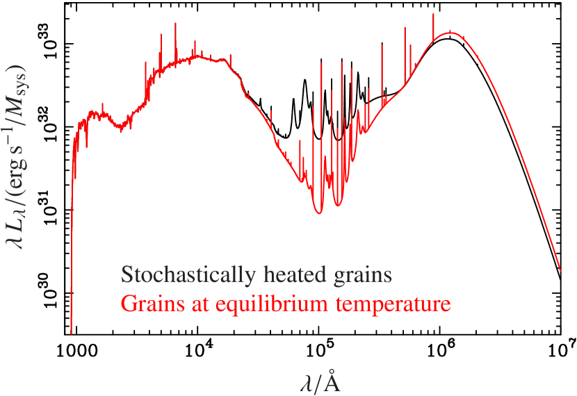
Figure 2: Effects of stochastic heating on the SED of the $13\mathclose{}\,\mathopen{}\mathrm{Gyr}$-old Milky Way model (see Sect. 7.1). All the SEDs shown hereafter were averaged over all viewing angles. For emission lines, only the peak was plotted; its height was computed assuming a Gaussian profile with a full width at half maximum of $160\mathclose{}\,\mathopen{}\mathrm{km/s}$ (Mocz et al., 2012). Black line: stochastically heated grains. Red line: all grains were assumed to have reached their equilibrium temperature.

By default, the self-absorption by dust grains of dust-emitted light is neglected. So, if one forgets star-forming clouds for the moment, the luminosity of a galaxy observed from an angle $\iota$ would just be $\Theta_{\lambda}(t,\iota)\mathclose{}\,\mathopen{}L^{0}_{\lambda}(t)+L^{\mathrm{d}}_{\lambda}(t)$ at time $t$. To assess the effects of self-absorption, a crude modeling of this phenomenon was however implemented in the code (see the documentation).

6 Star-forming regions and nebular emission

The code processes the clouds of interstellar matter surrounding star-forming regions separately from the diffuse interstellar medium (DISM). Star-forming clouds are modeled as homogeneous spherical shells of gas and dust, at the center of each of which resides a point-like cluster of young stars. The size of clouds is considered as negligible compared to that of the diffuse medium in which they are embedded; the emission emerging from any star-forming cloud is therefore subjected to the same processing by the DISM as that of the old stars scattered through the latter.

Because of the impact of massive stars on their surrounding, either through their intense radiation, stellar winds or supernova explosions, the life duration of star-forming clouds is a few million years at most. Young stars may also escape from their birth cloud before it is destroyed. The fraction $\varphi(t^{\prime})$ of stars aged $t^{\prime}$ still in their parent cloud is modeled as

$$\varphi(t^{\prime})=\varphi_{0}\mathclose{}\,\mathopen{}(1-t^{\prime}/\theta)^{\beta}\,\!,$$ (29)

where $\varphi_{0}$, $\theta$ and $\beta$ are constant parameters; $\varphi$ may also represent the covering factor of the cluster by the cloud, in which case a fraction $1-\varphi$ of the photons emitted by the cluster leak directly into the diffuse medium.

At any galactic age $t$, the code computes from the star formation rate $\psi(t-t^{\prime})$ the number of clusters with an age $t^{\prime}\leqslant\theta$ and the emission rate of Lyman continuum photons produced by each cluster, taking a typical initial stellar mass $M_{\textsc{sc}}$ for the clusters; this mass and the parameters $\varphi_{0}$, $\theta$ and $\beta$ mentioned above may be changed by the user.

6.1 Nebular emission from star-forming clouds. Dust effects on their SED

6.1.1 Nebular emission in the dust-free case

The modeling of nebular emission implemented in previous versions of Pégase dated back, for most of the emission lines, to Guiderdoni & Rocca-Volmerange (1987). The intensities of these lines were taken from Stasińska (1984), and only UV-to-near-IR lines at solar metallicity were considered. An upgrade was clearly needed.

We therefore computed a grid of models of dust-free H ii regions with version c17.01 of the code Cloudy (Ferland et al., 2017) as a function of the metallicity of the ISM, $Z_{\mathrm{mod}}$, and of the number rate of Lyman continuum (LC) photons emitted by the central ionizing source, $N_{\mathrm{mod}}$. The values considered ranged from $\mathord{\approx}\,0$ to $0.1$ for $Z_{\mathrm{mod}}$, and from $10^{46}$ to $10^{53}\mathclose{}\,\mathopen{}\mathrm{s}^{-1}$ for $N_{\mathrm{mod}}$.

The geometry adopted in these computations was radiation-bounded, spherical and with an inner cavity of radius $r_{\mathrm{c}}=1\mathclose{}\,\mathopen{}\mathrm{pc}$ centered on the ionizing source. The filling and covering factors were set to $1$ (their default value in Cloudy). The number density $n_{\mathrm{H}}$ of hydrogen atoms, be they neutral, ionized, isolated or in molecules, was assumed to be constant throughout the cloud. We took $n_{\mathrm{H}}=10^{2}\mathclose{}\,\mathopen{}\mathrm{cm}^{-3}$.

In addition to the amplitude of the ionizing radiation, characterized here by $N_{\mathrm{mod}}$, Cloudy needs its spectral shape. Because the exact shape only has a secondary impact on nebular emission, we did not use that of the star cluster at age $t^{\prime}$: this would have been very inconvenient as it would have required to precompute a huge grid of models for all ages and possible stellar initial mass functions. Instead, we took the unattenuated stellar emission produced by a constant star formation rate at fixed metallicity $Z_{\mathrm{mod}}$ and at an age $\mathord{\ga}\,10\mathclose{}\,\mathopen{}\mathrm{Myr}$. The reason for this is that the number rate of LC photons emitted by a single stellar population, $N_{\textsc{ssp}}(t^{\prime})$, drops very rapidly at $t^{\prime}>4\mathclose{}\,\mathopen{}\mathrm{Myr}$; so, the SED produced by a constant star formation rate does almost not evolve in the Lyman continuum at any age larger than $\mathord{\approx}\,10\mathclose{}\,\mathopen{}\mathrm{Myr}$. The resulting shape is a time-average of the ionizing SEDs, weighted by $N_{\textsc{ssp}}(t^{\prime})$; it should therefore be representative of the typical ionizing SED at the metallicity considered.

By default, Cloudy stops its calculations at the distance from the central source where the electronic temperature falls below $4000\mathclose{}\,\mathopen{}\mathrm{K}$. This criterion is not appropriate for low values of $N_{\mathrm{mod}}$ or high values of $Z_{\mathrm{mod}}$, as already mentioned in Moy (2000, sect. 3.4.4) and Gutkin et al. (2016), because this event occurs then well inside the H ii region: a large number of LC photons are not absorbed there yet, and the nebular emission predicted by the code with this criterion would therefore be unreliable. We instead required that Cloudy computes the state of the region up to the distance where the number density of free protons drops below $10^{-2}\mathclose{}\,\mathopen{}n_{\mathrm{H}}$.

For each model in the grid, we extracted from Cloudy’s outputs the integrated luminosity of emergent emission lines, out of which we selected all those brighter than $10^{-4}\leavevmode\nobreak\ \mathord{\times}$ the luminosity of Lyman $\alphaup$ in at least one of the models of the grid; this resulted in a final set of $\mathord{\approx}\,400$ lines, including many IR lines which were absent from Pégase.2. We also extracted the SED of the pure nebular continuum, uncontaminated by emission lines, and the value of the Strömgren radius of the model, $r_{\mathrm{S},\,0}^{\mathrm{mod}}$, defined as the distance to the cluster where the fraction of neutral hydrogen to all forms of hydrogen reaches $1/2$.

For each star cluster, Pégase.3 computes, in the dust-free case, the number rate of LC photons it emits at age $t^{\prime}$ which are absorbed by gas in the birth cloud as

$$N_{\textsc{bc}}(t^{\prime})=\varphi(t^{\prime})\mathclose{}\,\mathopen{}M_{\textsc{sc}}\mathclose{}\,\mathopen{}\left(\frac{N_{\textsc{ssp}}[t^{\prime}]}{M_{\textsc{ssp}}}\right)\!\,,$$ (30)

where $(N_{\textsc{ssp}}[t^{\prime}]/M_{\textsc{ssp}})$ is the number rate of LC photons emitted at age $t^{\prime}$ by an SSP, per unit mass of the SSP. It then interpolates in the $\{N_{\mathrm{mod}}\}\times\{Z_{\mathrm{mod}}\}$ space of cloud models at the point $(N_{\textsc{bc}}[t^{\prime}],Z[t])$ to compute, in the dust-free case, the Strömgren radius $r_{\mathrm{S},\,0}$ of the H ii region created in the cloud by the cluster, as well as the luminosities of the emission lines and of the nebular continuum produced there. More precisely, the code interpolates the nebular luminosities normalized to the LC luminosity (i.e., integrated over the Lyman continuum) of the model ionizing source, and scales these normalized luminosities by the fraction of the LC luminosity radiated by the cluster at age $t^{\prime}$ which is absorbed by gas in the birth cloud (this fraction is computed in the same way as the quantity $N_{\textsc{bc}}(t^{\prime})$ in Eq. (30)).

6.1.2 Dust effects

The H ii region surrounding a star cluster is also filled with dust which, because of the competition between gas and grains to absorb Lyman continuum photons, reduces the radius of the region from $r_{\mathrm{S},\,0}$ to $r_{\mathrm{S}}$. We assume that all the LC photons emitted by stars still in their parent cloud (or the photons not leaking directly in the diffuse medium, if $\varphi$ is interpreted as the covering factor of the cluster) are absorbed, either by gas or by dust, in the H ii region of the cloud. The volume reduction factor $\Upsilon$ is computed in a way similar to that in sect. 5.1.c of Spitzer (1978). Because the calculations in this book do no include any central cavity whereas Cloudy requires one, we had to adapt them; detailed explanations are provided in App. A. The intensities, when dust is present, of the nebular continuum and emission lines emerging from the cloud’s H ii region are then computed as $\Upsilon\leavevmode\nobreak\ \mathord{\times}$ their values in the dust-free case, while a fraction $1-\Upsilon$ of LC photons heat dust grains in this region.

However, because the Lyman $\alphaup$ line is resonant and has thus a large scattering optical depth in hydrogen, we assume that, as soon as any dust is present, all the photons emitted in this emission line are absorbed by grains, either in the cloud’s H ii region or in the neutral, H i region just surrounding it. The absorption of other emission lines and of the nebular continuum by dust in the H ii and H i regions of clouds is neglected.

Grains in the cloud’s H ii region also absorb a fraction of the non-ionizing photons emitted by the cluster. Because scattering by grains is mainly forward at the ultraviolet wavelengths where the cluster emits most of its light, we may estimate the fraction of stellar photons emerging from the H ii region, at a wavelength $\lambda$ longwards of the Lyman limit, as

$$\Theta_{\lambda}^{\textsc{bc}}\approx\exp\Bigl{(}-\kappa_{\lambda}^{\mathrm{abs}}[t]\mathclose{}\,\mathopen{}[r_{\mathrm{S}}-r_{\mathrm{c}}]\Bigr{)}.$$ (31)

The code finally determines the interstellar radiation field averaged over all star-forming clouds, using Eq. (26) with appropriate substitutions, and computes the emission of dust grains in clouds in the same way as explained in Sect. 5.2. Except for Lyman $\alphaup$, the very unconstrained absorption of the stellar and nebular emission by dust in the H i regions of clouds is not taken into account. As an example, we compare in Fig. 3 the mean radiation field in the diffuse ISM and in star-forming clouds for the Milky Way model described in Sect. 7.1.

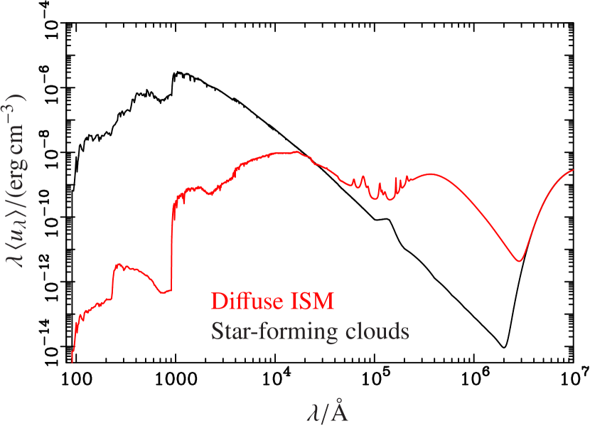
Figure 3: Mean radiation field of the $13\mathclose{}\,\mathopen{}\mathrm{Gyr}$-old Milky Way model in star-forming clouds (black line) and in the diffuse interstellar medium (red line). The quantity $\langle u_{\lambda}\rangle$ is the energy density. The bump at long wavelengths is the cosmic microwave background.

6.2 Nebular emission by the diffuse ISM

A fraction $1-\varphi(t^{\prime})$ of the Lyman continuum photons emitted by a single stellar population with an age $t^{\prime}$ are produced in the diffuse interstellar medium (or have leaked into it, if $\varphi$ is interpreted as the covering factor of the cluster by the birth cloud). We assume that all these photons are absorbed in the DISM. The spherical geometry adopted to model star-forming clouds is obviously not suitable to compute the nebular emission of the diffuse medium. However, because the ionization parameter $U$ is the main determinant (besides metallicity) of the intensity of emission lines and of the nebular continuum (Davidson, 1977), we may reuse the results obtained for dust-free clouds and take, as a proxy and with some appropriate scaling, the nebular emission of a cloud with a mean value of $U$ equal to that of the DISM. A typical value of the latter is $U_{\textsc{dism}}\approx 10^{-3.5}$, according to Flores-Fajardo et al. (2011) (see also Dopita et al., 2006).

So, for each model of cloud in the grid described in Sect. 6.1.1, we computed the average $\langle U_{\mathrm{mod}}\rangle$ of the ionization parameter over the volume of the H ii spherical shell surrounding the central cluster (Charlot & Longhetti, 2001) as follows: at a distance $r$ from the central source, the ionization parameter is

$$U_{\mathrm{mod}}(r)=\frac{N_{\mathrm{mod}}}{4\mathclose{}\,\mathopen{}\pi\mathclose{}\,\mathopen{}r^{2}\mathclose{}\,\mathopen{}n_{\mathrm{H}}\mathclose{}\,\mathopen{}c}\,,$$ (32)

so

$$\langle U_{\mathrm{mod}}\rangle=\frac{3\mathclose{}\,\mathopen{}N_{\mathrm{mod}}}{4\mathclose{}\,\mathopen{}\pi\mathclose{}\,\mathopen{}n_{\mathrm{H}}\mathclose{}\,\mathopen{}c}\mathclose{}\,\mathopen{}\frac{r_{\mathrm{S},\,0}^{\mathrm{mod}}-r_{\mathrm{c}}}{\Bigl{(}r_{\mathrm{S},\,0}^{\mathrm{mod}}\Bigr{)}^{3}-r_{\mathrm{c}}^{3}}.$$ (33)

Pégase.3 interpolates then in the $\{\langle U_{\mathrm{mod}}\rangle\}\times\{Z_{\mathrm{mod}}\}$ space of cloud models at the point $(U_{\textsc{dism}},Z[t])$ to compute the nebular emission produced by a cloud in nearly the same state as the diffuse medium at age $t$; this typically corresponds to a cloud model with $N_{\mathrm{mod}}\approx 10^{47}\mathclose{}\,\mathopen{}\mathrm{s}^{-1}$. Finally, to obtain the overall nebular emission of the DISM, the code scales the luminosities of the emission lines and of the nebular continuum emerging from the “interpolated” cloud by the ratio of the LC luminosity radiated at time $t$ by stars in the diffuse medium to that of the ionizing source of the cloud.

As with star-forming clouds, we assume that all the photons emitted in the Lyman $\alphaup$ line by the DISM are absorbed by grains as soon as any dust is present. The other emission lines and the nebular continuum produced in the diffuse medium are attenuated in the same way as stars in the latter.

7 Main outputs

For each scenario, the code provides a large number of outputs as a function of galactic age: masses and SEDs of various components, chemical abundances, star formation and supernova rates. We refer to the code’s documentation for a detailed list of all the quantities. In the following, we present some outputs obtained for a scenario fitted to observed colors of nearby spiral galaxies of Sbc Hubble type. As this is the most likely type for the Milky Way (de Vaucouleurs & Pence, 1978; Hodge, 1983), we also constrained this scenario using observed properties of the MW’s local ISM and call it the “MW model”.

7.1 Abundances of metallic elements

Figure 4 shows the evolution of the ISM abundances of several elements for the MW model. These abundances are compared at $\mathord{\approx}\,13\mathclose{}\,\mathopen{}\mathrm{Gyr}$ with observed abundances in the solar neighborhood from Anders & Grevesse (1989).

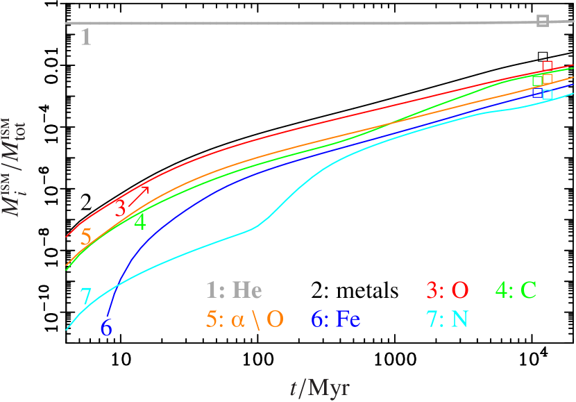
Figure 4: Evolution of ISM abundances as a function of galactic age $t$ for the Milky Way model (lines): $M_{i}^{\textsc{ism}}$ is the mass in the ISM of the element (or elements) referred to by the index $i$, and $M_{\mathrm{tot}}^{\textsc{ism}}$ is the total mass of the ISM; “metals” denotes the sum on all metals, and “$\alphaup\setminus\mathrm{O}$”, the sum on Ne, Mg, Si, S and Ca. Squares are the corresponding observed abundances of Anders & Grevesse (1989) (shuffled around $13\mathclose{}\,\mathopen{}\mathrm{Gyr}$ for the sake of clarity).

The scenario used for the MW model was the following: the galaxy assembles by infall at an exponentially decreasing rate, with a timescale of $6\mathclose{}\,\mathopen{}\mathrm{Gyr}$; there are no galactic outflows; the star formation rate is proportional to the current mass of the ISM, with an efficiency of $(6\mathclose{}\,\mathopen{}\mathrm{Gyr})^{-1}$; the IMF is from Kroupa et al. (1993); the chemical yields by massive stars are from Portinari et al. (1998); the values adopted to model star-forming clouds are $M_{\textsc{sc}}=10^{4}\mathclose{}\,\mathopen{}M_{\odot}$, $\varphi_{0}=1$, $\theta=10\mathclose{}\,\mathopen{}\mathrm{Myr}$ and $\beta=1$.

7.2 SEDs and colors

Galaxy SEDs are computed on the wavelength domain defined jointly by the library of stellar spectra and the model of grains, continuously from the far-UV to the far-IR and submm. The spectral resolution decreases from $\lambda/\Delta\lambda\approx 100$ in the far-UV to $\mathord{\approx}\,20$ in the submm.

More than $60$ calibrated filter passbands are provided with the code. Other filters may easily be added to this list, as long as the reference spectrum used for the calibration (e.g., Vega, AB) and the passband transmission (whether in energy or in number of photons) are known. Magnitudes are calculated from the galaxy SED through all these passbands. The user may freely select the magnitudes, luminosities, colors and line equivalent widths printed by the code.

As an illustration, we compare, in Table 2 and Fig. 5, the near-UV-to-near-IR colors and spectrum of the Milky Way model at $t=13\mathclose{}\,\mathopen{}\mathrm{Gyr}$ with typical total observed colors of nearby Sbc galaxies. The model spectrum was computed with the BaSeL-2.2 library of stellar spectra and averaged over all viewing angles. The observed $B-H$, $J-H$ and $H-K$ colors were compiled by Fioc & Rocca-Volmerange (1999a), corrected for aperture and redshift, and gathered in eight types covering the whole Hubble sequence, one of which being the Sbc type discussed here; the authors also averaged these colors within each of these types according to a procedure (described in their paper) taking into account uncertainties and the intrinsic scatter. The $U-B$ and $B-V$ (resp. $V-R_{\mathrm{c}}$ and $V-I_{\mathrm{c}}$) mean observed colors of the same morphological types were computed from the data in de Vaucouleurs (1991) (resp. Buta & Williams, 1995); we submitted them to the same averaging procedure than $B-H$ and near-IR colors.

Table 2: Comparison of near-UV-to-near-IR colors of the MW model at $t=13\mathclose{}\,\mathopen{}\mathrm{Gyr}$ with typical total observed colors of nearby Sbc galaxies computed by Fioc & Rocca-Volmerange (1999a). (See Sects. 7.1 and 7.2 for details.)

Color	Average observed Sbc	MW model
$B-V$	$0.63$	$0.634$
$U-B$	$0.04$	$0.056$
$V-R_{\mathrm{c}}$	$0.48$	$0.509$
$V-I_{\mathrm{c}}$	$1.01$	$1.088$
$J-H$	$0.77$	$0.750$
$H-K$	$0.22$	$0.307$
$B-H$	$3.33$	$3.408$

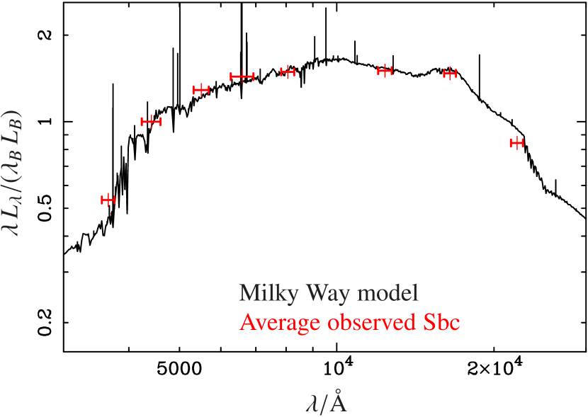
Figure 5: Near-UV-to-near-IR spectral energy distribution of the $13\mathclose{}\,\mathopen{}\mathrm{Gyr}$-old Milky Way model (black line), compared with the mean observed fluxes of local Sbc galaxies (red crosses) in the $U$, $B$, $V$, $R_{\mathrm{c}}$, $I_{\mathrm{c}}$, $J$, $H$ and $K$ passbands (see Sects. 7.1 and 7.2 for details). All fluxes were normalized to the $B$ band. The red horizontal segments correspond to the width of the passbands. See also Table 2.

7.3 Evolution of the SED and of galactic components

In addition to the overall SED of a galaxy, the code may on request separately output the SEDs of its several components – stars, ionized gas, dust species –, whether in the diffuse medium or in star-forming regions. This is illustrated by Fig. 6 for the Milky Way model at $t=13\mathclose{}\,\mathopen{}\mathrm{Gyr}$.

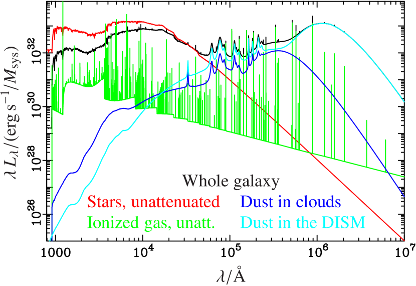
Figure 6: Spectral energy distribution of the $13\mathclose{}\,\mathopen{}\mathrm{Gyr}$-old Milky Way model (black line) and of its components: unattenuated nebular continuum and lines produced by the ionized gas (green line); dust emission from star-forming clouds (dark blue line); dust emission from the diffuse ISM (light blue line). The unattenuated stellar continuum is plotted in red.

At this late age, UV-to-near-IR wavelengths are dominated by the attenuated light of stars, with a negligible contribution from the nebular continuum, and mid-IR-to-submm wavelengths are dominated by dust grains. Whereas the emission of grains in star-forming clouds is of the same order of magnitude in the mid-IR as that of grains in the diffuse ISM, the contribution of the latter is overwhelming in the far-IR/submm domain and in the overall emission of dust, as may be seen in Fig. 7.

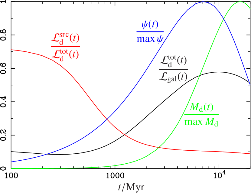
Figure 7: Evolution, as a function of galactic age $t$, of the following quantities for the Milky Way model: star formation rate $\psi(t)$ (relative to its maximal value); dust mass $M_{\mathrm{d}}(t)$ (idem); ratio of the bolometric luminosity emitted by dust in the whole galaxy, $\mathcal{L}_{\mathrm{d}}^{\mathrm{tot}}(t)$, to the overall bolometric luminosity of the galaxy, $\mathcal{L}_{\mathrm{gal}}(t)$; ratio of the bolometric luminosity emitted by dust in star-forming clouds, $\mathcal{L}_{\mathrm{d}}^{\textsc{sfc}}(t)$, to $\mathcal{L}_{\mathrm{d}}^{\mathrm{tot}}(t)$.

The evolution of the Milky Way model’s SED is plotted in Fig. 8 from the far-UV to submm wavelengths.

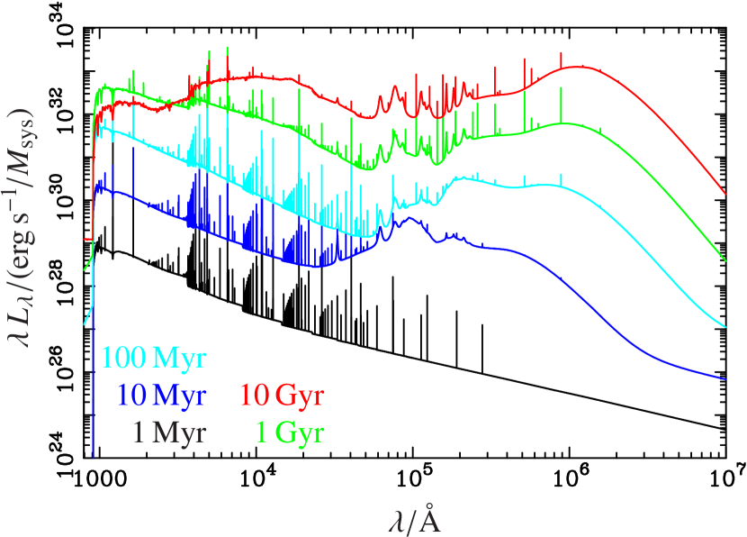
Figure 8: Spectral energy distribution of the Milky Way model at various ages (color coded on the plot).

We analyze it below with the help of Fig. 7, where we have plotted, for the same scenario, the evolution as a function of age of the following quantities: the ratio of the bolometric luminosity radiated by dust grains in all regions of the galaxy, $\mathcal{L}_{\mathrm{d}}^{\mathrm{tot}}(t)$, to the bolometric luminosity of the whole galaxy (stars, gas and dust), $\mathcal{L}_{\mathrm{gal}}(t)$; the ratio of the bolometric luminosity radiated by grains in star-forming clouds, $\mathcal{L}_{\mathrm{d}}^{\textsc{sfc}}(t)$, to $\mathcal{L}_{\mathrm{d}}^{\mathrm{tot}}(t)$; the dust mass $M_{\mathrm{d}}(t)$; the star formation rate $\psi(t)$. (The last two quantities are normalized to their maximal values.)

Three trends appearing in Fig. 8 deserve to be especially emphasized: Firstly, the luminosity increases in the UV and, even more, in the optical–near-IR domain until late ages. This happens because the modeled galaxy assembles by infall on a long timescale: the star formation rate (SFR) being regulated by the mass of gas available in the ISM, it initially increases during several $\mathrm{Gyr}$ (see Fig. 7) and then decreases only slowly; as a result, in this model, the rapid decline of the luminosity of a single stellar population is more than balanced by the accumulation of successive stellar generations, and the overall luminosity grows steadily at wavelengths dominated by stars.

Secondly, the spectrum progressively reddens from the UV to the near-infrared, due to the aging of the bulk of the stellar population and to the increasing metallicity of the ISM from which stars form. In parallel, the discontinuities of the nebular continuum are more and more swamped in the stellar emission, up to the point, after $1\mathclose{}\,\mathopen{}\mathrm{Gyr}$, where they are not discernible anymore.

Lastly, at longer wavelengths, the most noticeable feature is the shift of the infrared peak from $\lambda\simeq 10\mathclose{}\,\mathopen{}\mathrm{\muup m}$ at an age of $10\mathclose{}\,\mathopen{}\mathrm{Myr}$ to more than $100\mathclose{}\,\mathopen{}\mathrm{\muup m}$ at $10\mathclose{}\,\mathopen{}\mathrm{Gyr}$. (Note that this peak is distinct from the near-IR peak observed around $\lambda\in[1,2]\mathclose{}\,\mathopen{}\mathrm{\muup m}$ at late ages (see Fig. 8): the latter is caused by evolved low-mass cold giant stars.) At young ages, most of the emission by dust comes from grains in star-forming regions, heated to very high temperatures by the UV photons produced by nearby young luminous stars, and reradiating in the mid-IR. After $1\mathclose{}\,\mathopen{}\mathrm{Gyr}$, most of the dust emission is due to grains in the diffuse ISM and radiating in the far-IR (see the red curve in Fig. 7).

The reasons for this behavior are the following: As time progresses, the total mass in the old and intermediate-age stars dominating optical wavelengths and scattered through the whole galaxy grows. The radiation field produced by these stars becomes therefore more intense. It is however softer than in star-forming regions (see Fig. 3), so grains in the diffuse medium reach colder temperatures and emit at longer wavelengths. In parallel, the ISM is enriched by the ejecta of previous stellar generations, and its metallicity constantly increases. The mass of the ISM grows until $\mathord{\approx}\,7\mathclose{}\,\mathopen{}\mathrm{Gyr}$ (see the blue curve in Fig. 7: we remind the reader that, for the star formation law adopted in the Milky Way model, the ISM mass is proportional to the SFR $\psi(t)$). The mass of metals in the ISM, which is equal to the product of the metallicity of the ISM by the mass of the latter, peaks therefore later than the SFR. The same holds consequently for the mass of dust (green curve in Fig. 7). The ratio of $\mathcal{L}_{\mathrm{d}}^{\mathrm{tot}}(t)$ to $\mathcal{L}_{\mathrm{gal}}(t)$ (black curve) – which depends on recent star formation, on the mass in older stars and on that of dust – reaches its maximum at an age between the peak ages of the SFR and of the mass of dust.

7.4 Temperatures and SEDs of grains

Pégase.3 may optionally provide the temperature probability distribution of stochastically heated individual grains and their emission spectrum. As an illustration, Fig. 9 shows these properties for silicate grains with various radii in the diffuse ISM of the Milky Way model at $13\mathclose{}\,\mathopen{}\mathrm{Gyr}$.

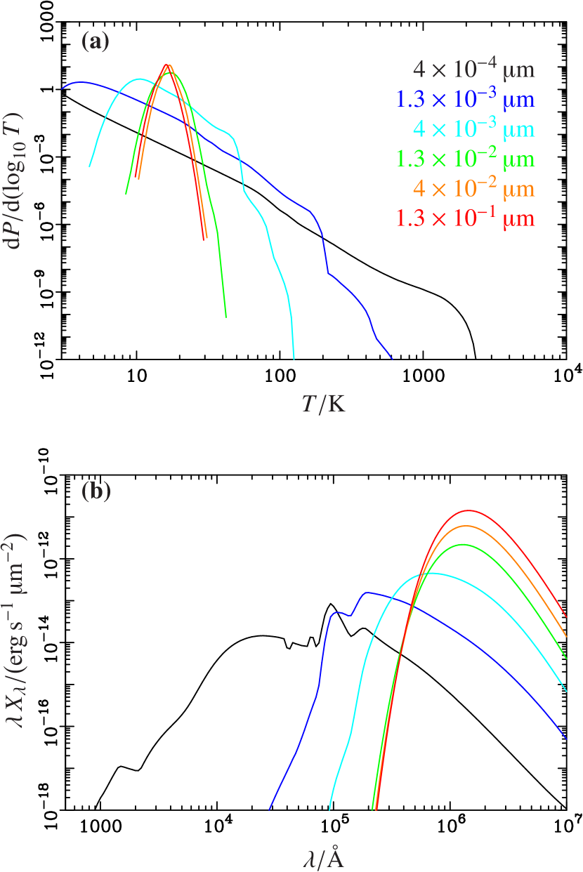
Figure 9: (a) Temperature probability distribution of silicate grains in the diffuse medium of the $13\mathclose{}\,\mathopen{}\mathrm{Gyr}$-old Milky Way model. Grain radii are color coded as indicated on the plot. (b) Emission spectra of these grains (same color coding for grain radii as in previous subfigure). The quantity $X_{\lambda}$ is the spectral exitance (luminosity per unit surface of the grain).

This figure highlights that small grains have a large range of temperatures and emit significantly at short wavelengths. For bigger and bigger grains, the temperature distribution narrows around the equilibrium value, and the emission spectrum becomes similar to that of a blackbody peaking in the far-IR.

The SEDs of the several species of dust grains – silicates, graphites and PAHs – are plotted in Fig. 10 for the same model. While PAH features are prominent in the mid-IR, graphites dominate at longer wavelengths. Only in the submillimeter domain are silicates major contributors to the global SED.

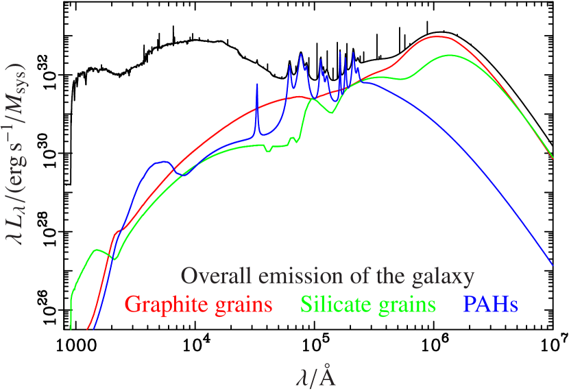
Figure 10: Spectral energy distributions of the several species of dust grains (graphites, red line; silicates, green line; PAHs, blue line) and of the whole galaxy (black line) for the $13\mathclose{}\,\mathopen{}\mathrm{Gyr}$-old Milky Way model.

8 Conclusion and prospects

This paper presents Pégase.3, a new version of the code Pégase specifically aimed to model the spectrochemical evolution of galaxies at all redshifts. The most important outputs of the code are synthetic SEDs from the far-UV to the submillimeter, from which colors may be determined in a large number of photometric systems. Because the star formation history and the chemical evolution are computed consistently, this large wavelength range should help to lessen the degeneracy between the parameters (e.g., stellar mass, current SFR, age, metallicity) derived from fits of model SEDs to galaxy observations.

The main improvement, with respect to previous versions of the code, is the extension to the mid- and far-infrared, which required to model the evolution of the dust content and its effects on the light radiated by a galaxy. The computation of the nebular emission, in particular of metallic and infrared lines, has also been entirely upgraded using Cloudy.

To determine the amount of carbonaceous and silicate grains, Pégase now follows the detailed evolution of the abundances of the most important elements in the interstellar medium. To this purpose, two models are proposed in the code: a phenomenological one in which the mass of grains is directly related to the amount of their constituents in the ISM; a more physical one, based on Dwek (1998) and fitted by him to Milky Way data, in which dust grains form in the circumstellar envelopes of stars and around supernovae, accrete on grains already present in the ISM and are destroyed by supernovae blast waves in the ISM.

The overall optical properties of dust are then computed, assuming some size distributions for the various species of grains. These optical properties are used to obtain the attenuation through the diffuse interstellar medium of the stellar and nebular light at all wavelengths, using grids of radiative transfer for geometries appropriate to either spheroidal galaxies or spiral disks and bulges. All these grids were computed beforehand with Monte Carlo simulations based on the method of virtual interactions. The attenuation by dust in their birth cloud of the light emitted by young stars, in particular in the Lyman continuum, is also estimated.

The advantage of this procedure is that it also provides the mean radiation field in the diffuse medium and the one averaged over all star-forming clouds. The re-emission by dust of the energy it absorbed is then computed from the optical properties of individual grains, taking into account their stochastic heating by the mean radiation field in the two regions.

In spite of some limitations (use of mean radiation fields, self-absorption by dust grains not rigorously treated), the method implemented in Pégase to compute far-UV-to-submm SEDs is more physical than in other codes, where the shape of the radiation field does not evolve (e.g., Galliano et al., 2011), or which use template attenuation curves unrelated to the dust content (for instance, the one determined for starbursts by Calzetti et al., 1994) or template infrared SEDs (e.g., graybodies, as in da Cunha et al., 2008, or the semi-empirical SEDs of Dale et al., 2014). It is beyond the scope of this paper to compare Pégase.3 to all these codes, but, to highlight the specifities of ours, let us just consider a recent one, Cigale (Boquien et al., 2019, in its last version). The working principle of this code is quite different from that of Pégase.3, despite similar goals, as, when fitting modeled SEDs to an object’s observed spectral data, Cigale employs a powerful Bayesian method to derive the likelihood of the input parameters. However, in this procedure, the various galactic components – stars, gas and dust – are treated independently. For instance, the metallicity of stellar populations is constant, and the star formation history is quite arbitrary since neither the evolution of the ISM nor the history of mass assembly of the galaxy are considered. The only theoretical constraint is that the energy balance between the absorption of stellar and nebular light by dust and its re-emission must be respected. This data-driven approach provides a lot of suppleness but does not ensure the internal consistency of the models. On the other hand, although Pégase.3 does not incorporate a fitting procedure of the code’s scenarios to observed data, it strives to model simultaneously the evolution of stellar populations and of gas and dust in the ISM, in particular the abundances of various metals and types of grains, as well as the contributions of these components to the SED. Finally, Cigale relies on libraries of single stellar populations computed by either Bruzual & Charlot (2003) or Maraston (2005); in contrast to Pégase, users of this code do not, therefore, have full control of these inputs and are restricted to a limited number of initial mass functions.

Codes more sophisticated than Pégase in some respects also exist. For instance, Grasil (Granato et al., 2000) takes into account the radiation field at each point in the galaxy and the self-absorption by dust grains. This, however, requires users to run anew Monte Carlo simulations of radiative transfer at all ages, for each modeled galaxy, which seems impractical to simulate the evolution of a large number of objects on cosmological timescales. To fulfill this aim, the choice made in Pégase.3 was rather to try to strike the right balance between computational efficiency and physical correctness, while still maintaining consistency of the modeling.

The code provides a wealth of outputs, besides SEDs and derived quantities (colors, equivalent widths of emission lines, etc.): among others, the masses in stars, compact stellar remnants, the ISM and dust grains; the abundances of the most important elements; the rates of star formation, ionizing photon emission and supernova explosions, both for core-collapse and type Ia objects. Because of the large amount of space they would occupy, other outputs are only optional, such as the separate SEDs emitted by dust species, the mean radiation fields in the diffuse medium and in star-forming clouds, or, even more, the temperature distributions and SEDs of individual grains. Some of these outputs were illustrated in this paper for the “Milky Way” model.

Preliminary versions of Pégase.3 were also used to study spheroidal galaxies. In particular, Rocca-Volmerange et al. (2013) analyzed the SEDs of radiogalaxy hosts observed by HST, Spitzer and Herschel at redshifts $z\in[1,5]$; the authors showed that these distant objects were already old then ($\text{age}\geqslant 1\mathclose{}\,\mathopen{}\mathrm{Gyr}$), massive (stellar mass $\mathord{\sim}\,10^{11}$ to $10^{12}\mathclose{}\,\mathopen{}M_{\odot}$) and that they had recently undergone an extended burst of star formation. Drouart et al. (2016) and Podigachoski et al. (2016) also used Pégase.3, in combination with models of AGNs, to disentangle the contributions of an active nucleus and of dust heated by young stars to the mid- and far-IR emission.

Because of its large spectral coverage, the code provides a nearly “bolometrically”-complete modeling for standard galaxies. This will make it possible to study in a more consistent way the star formation history, the dust attenuation and emission and the chemical evolution in these objects, and to build more-reliable indicators of the recent star formation rate, stellar mass, age, metallicity and dust content.

The flexibility of the code and the variety of the scenarios that may be input should be of particular interest for cosmological simulations. For instance, the stellar initial mass function and the parameters of the laws giving the star formation, infall and outflow rates may easily be changed. Users may also provide a file giving these rates at some ages, from which the code interpolates at intermediate ages. They may even define several episodes of star formation, infall and outflow, whether consecutive or overlapping, and modulate the star formation rate stochastically.

The current spectral resolution of model SEDs is low but will be improved in the near future by our team. We also intend to implement in Pégase more-realistic models of dust grain composition and evolution, such as the one built with Themis (Jones et al., 2017), and more-modern sets of stellar evolutionary tracks, spectra and chemical yields. However, in view of analyzing forthcoming infrared data, for example those that the SPICA space observatory will provide (Fernández-Ontiveros et al., 2017) if selected for launch, our main effort will concentrate on the modeling of star-forming regions, in particular the competition between gas and dust in H ii regions to absorb ionizing photons and the effects of grains on nebular emission.

Appendix A Adaptation of the calculations by Spitzer (1978) to the case of an inner cavity

Here, we consider the H ii region created by a point-like star cluster in a cloud of gas and dust. Except for a spherical inner cavity of radius $r_{\mathrm{c}}$ centered on the cluster, the cloud is assumed to be homogeneous: the overall number density $n_{\mathrm{H}}$ of hydrogen atoms, whether neutral or ionized, is constant, as is the dust-to-gas ratio. In the dust-free case, we already know from the Cloudy results (see Sect. 6.1.1) the value of the Strömgren radius $r_{\mathrm{S},\,0}$, that is, the outer radius of the spherical shell of ionized hydrogen. Our goal here is to estimate the Strömgren radius $r_{\mathrm{S}}$ ($\mathord{<}\,r_{\mathrm{S},\,0}$) when dust is present, and, from that, the fraction $\Upsilon$ of Lyman continuum photons absorbed in the cloud by gas rather than by dust. To this purpose, we have adapted to the case where an inner cavity is present in the H ii region the calculations in sect. 5.1.c of Spitzer (1978); we refer in the following to the equations in this work by prefixing the characters “Sp.” to the equation number.

Let us first restate the most important assumptions and simplifications made in Spitzer (1978):

1. The H ii region contains only hydrogen and dust;

2. The H ii region is ionization-bounded, and the transition zone from the almost fully ionized medium to the neutral one is very thin;

3. All Lyman continuum photons are considered to be at a frequency just above the Lyman limit;

4. The standard case B (see Osterbrock & Ferland 2006, sect. 4.2) holds for the recombination of hydrogen.

Because the asymmetry parameter is close to $1$ at short wavelengths, we moreover assume here that dust scattering is only forward. This does not make the calculations more complicated since one just has to replace the mass extinction coefficient of dust, $\kappa_{\mathrm{d}}^{\mathrm{ext}}$, by the absorption one, $\kappa_{\mathrm{d}}^{\mathrm{abs}}$. Some of these approximations and assumptions are highly debatable, but, given all the uncertainties on the physics of dusty H ii regions (the sublimation of grains, among others), a more complicated modeling does not seem to be worthwhile for this paper.

The probability per unit time that a given hydrogen atom at a distance $r$ from the cluster becomes ionized is

$$p(r)=\frac{\kappa_{\mathrm{H}}\mathclose{}\,\mathopen{}N\mathclose{}\,\mathopen{}\mathrm{e}^{-\tau(r)}}{4\mathclose{}\,\mathopen{}\pi\mathclose{}\,\mathopen{}r^{2}}\,,\qquad\text{(Sp.\leavevmode\nobreak\ 5-24)}$$ (42)

where $\kappa_{\mathrm{H}}$ is the ionizing cross-section of an hydrogen atom, $N$ is the number rate of Lyman continuum photons emitted by the central source, and $\tau(r)$ is the absorption optical depth by both hydrogen and dust from the source up to the distance $r$. The ionization balance is given by

$$(1-\xi[r])\mathclose{}\,\mathopen{}p(r)=\xi(r)\mathclose{}\,\mathopen{}n_{\mathrm{e}}(r)\mathclose{}\,\mathopen{}\alpha_{\mathrm{B}}(r)\,,\qquad\text{(Sp.\leavevmode\nobreak\ 5-2)}$$ (43)

where $\xi(r)$ is the fraction of ionized hydrogen atoms, $n_{\mathrm{e}}(r)$ is the number density of electrons, and $\alpha_{\mathrm{B}}(r)$ is the case B recombination coefficient for hydrogen. Since $n_{\mathrm{e}}(r)=\xi(r)\mathclose{}\,\mathopen{}n_{\mathrm{H}}$ and $\xi(r)\approx 1$ in the H ii region, one may rewrite Eq. (43) as

$$(1-\xi[r])\mathclose{}\,\mathopen{}p(r)\approx n_{\mathrm{H}}\mathclose{}\,\mathopen{}\alpha_{\mathrm{B}}\,,$$ (44)

where $\alpha_{\mathrm{B}}$ is now treated as a constant throughout the ionized medium.

The absorption optical depth by hydrogen $\tau_{\mathrm{H}}(r)$ from the source up to the distance $r$ obeys the relation

$$\mathrm{d}\tau_{\mathrm{H}}=(1-\xi[r])\mathclose{}\,\mathopen{}n_{\mathrm{H}}\mathclose{}\,\mathopen{}\kappa_{\mathrm{H}}\mathclose{}\,\mathopen{}\mathrm{d}r.\qquad\text{(Sp.\leavevmode\nobreak\ 5-16)}$$ (45)

With an inner cavity, eq. (Sp. 5-21) becomes

$$N=\frac{4\mathclose{}\,\mathopen{}\pi}{3}\mathclose{}\,\mathopen{}\Bigl{(}r_{\mathrm{S},\,0}^{3}-r_{\mathrm{c}}^{3}\Bigr{)}\mathclose{}\,\mathopen{}\langle n_{\mathrm{e}}\mathclose{}\,\mathopen{}n_{\mathrm{p}}\mathclose{}\,\mathopen{}\alpha_{\mathrm{B}}\rangle\approx\frac{4\mathclose{}\,\mathopen{}\pi}{3}\mathclose{}\,\mathopen{}\Bigl{(}r_{\mathrm{S},\,0}^{3}-r_{\mathrm{c}}^{3}\Bigr{)}\mathclose{}\,\mathopen{}n_{\mathrm{H}}^{2}\mathclose{}\,\mathopen{}\alpha_{\mathrm{B}}\,,$$ (46)

where $\langle\cdot\rangle$ denotes a volume-average and $\xi$ has been approximated to $1$ in the H ii region.

Combining Eqs. (42), (44) and (46), one obtains

$$(1-\xi[r])\mathclose{}\,\mathopen{}\kappa_{\mathrm{H}}\mathclose{}\,\mathopen{}n_{\mathrm{H}}\mathclose{}\,\mathopen{}r_{\mathrm{S},\,0}=\frac{3\mathclose{}\,\mathopen{}\mathrm{e}^{\tau(r)}\mathclose{}\,\mathopen{}\gamma^{2}(r)}{1-\gamma_{\mathrm{c}}^{3}}\,,$$ (47)

with $\gamma(r)\coloneqq r/r_{\mathrm{S},\,0}$ and $\gamma_{\mathrm{c}}\coloneqq\gamma(r_{\mathrm{c}})$. Since

$$\mathrm{d}\tau_{\mathrm{H}}=(1-\xi[r])\mathclose{}\,\mathopen{}\kappa_{\mathrm{H}}\mathclose{}\,\mathopen{}n_{\mathrm{H}}\mathclose{}\,\mathopen{}r_{\mathrm{S},\,0}\mathclose{}\,\mathopen{}\mathrm{d}\gamma$$ (48)

from Eq. (45) and the definition of $\gamma$, one obtains from Eqs. (47) and (48) that

$$\mathrm{d}\tau_{\mathrm{H}}=\frac{3\mathclose{}\,\mathopen{}\mathrm{e}^{\tau(r)}\mathclose{}\,\mathopen{}\gamma^{2}(r)}{1-\gamma_{\mathrm{c}}^{3}}\mathclose{}\,\mathopen{}\mathrm{d}\gamma.$$ (49)

Let $\tau_{\mathrm{d}}(r)$ be the absorption optical depth by dust from the source up to the distance $r$. One has

$$\tau_{\mathrm{d}}(r)=\kappa_{\mathrm{d}}^{\mathrm{abs}}\mathclose{}\,\mathopen{}\mu_{\mathrm{d}}\mathclose{}\,\mathopen{}(r-r_{\mathrm{c}})=(\gamma[r]-\gamma_{\mathrm{c}})\mathclose{}\,\mathopen{}\zeta\,,$$ (50)

where $\mu_{\mathrm{d}}$ is the mass density of dust in the H ii region (related to $n_{\mathrm{H}}$ by the dust-to-hydrogen ratio derived from the evolution of the galaxy), and

$$\zeta\coloneqq\kappa_{\mathrm{d}}^{\mathrm{abs}}\mathclose{}\,\mathopen{}\mu_{\mathrm{d}}\mathclose{}\,\mathopen{}r_{\mathrm{S},\,0}.$$ (51)

Since $\tau(r)=\tau_{\mathrm{H}}(r)+\tau_{\mathrm{d}}(r)$, Eq. (49) gives

$$\mathrm{e}^{-\tau_{\mathrm{H}}(r)}\mathclose{}\,\mathopen{}\mathrm{d}\tau_{\mathrm{H}}=\frac{3\mathclose{}\,\mathopen{}\mathrm{e}^{\tau_{\mathrm{d}}(r)}\mathclose{}\,\mathopen{}\gamma^{2}(r)}{1-\gamma_{\mathrm{c}}^{3}}\mathclose{}\,\mathopen{}\mathrm{d}\gamma.$$ (52)

To compute $r_{\mathrm{S}}$, let us integrate this equation from $r_{\mathrm{c}}$ to $r_{\mathrm{S}}$, as in Spitzer (1978). The left-hand side is

$$\int_{\tau_{\mathrm{H}}(r)=\tau_{\mathrm{H}}(r_{\mathrm{c}})}^{\tau_{\mathrm{H}}(r_{\mathrm{S}})}\mathrm{e}^{-\tau_{\mathrm{H}}(r)}\mathclose{}\,\mathopen{}\mathrm{d}\tau_{\mathrm{H}}=\mathrm{e}^{-\tau_{\mathrm{H}}(r_{\mathrm{c}})}-\mathrm{e}^{-\tau_{\mathrm{H}}(r_{\mathrm{S}})}\approx 1\,,$$ (53)

since $\tau_{\mathrm{H}}(r_{\mathrm{c}})=0$ and (by definition of $r_{\mathrm{S}}$) $\tau_{\mathrm{H}}(r_{\mathrm{S}})\gg 1$. The value of $\gamma_{\mathrm{S}}\coloneqq\gamma(r_{\mathrm{S}})$ is therefore the unique solution in the interval $[\gamma_{\mathrm{c}},1]$ of $f(\gamma_{\mathrm{S}})=0$, with

$$\!f(\gamma_{\mathrm{S}}) \coloneqq\frac{3\mathclose{}\,\mathopen{}\mathrm{e}^{-\gamma_{\mathrm{c}}\mathclose{}\,\mathopen{}\zeta}}{1-\gamma_{\mathrm{c}}^{3}}\mathclose{}\,\mathopen{}\int_{\gamma=\gamma_{\mathrm{c}}}^{\gamma_{\mathrm{S}}}\mathrm{e}^{\gamma\mathclose{}\,\mathopen{}\zeta}\mathclose{}\,\mathopen{}\gamma^{2}\mathclose{}\,\mathopen{}\mathrm{d}\gamma-1$$

$$=3\mathclose{}\,\mathopen{}\frac{\mathrm{e}^{\varepsilon_{\mathrm{S}}-\varepsilon_{\mathrm{c}}}\mathclose{}\,\mathopen{}\bigl{(}\varepsilon_{\mathrm{S}}^{2}-2\mathclose{}\,\mathopen{}\varepsilon_{\mathrm{S}}+2\bigr{)}-\bigl{(}\varepsilon_{\mathrm{c}}^{2}-2\mathclose{}\,\mathopen{}\varepsilon_{\mathrm{c}}+2\bigr{)}}{\bigl{(}1-\gamma_{\mathrm{c}}^{3}\bigr{)}\mathclose{}\,\mathopen{}\zeta^{3}}-1\,,$$ (54)

where $\varepsilon_{\mathrm{S}}\coloneqq\gamma_{\mathrm{S}}\mathclose{}\,\mathopen{}\zeta$ and $\varepsilon_{\mathrm{c}}\coloneqq\gamma_{\mathrm{c}}\mathclose{}\,\mathopen{}\zeta$. For $\zeta\ll 1$, the evaluation of $f(\gamma_{\mathrm{S}})$ is numerically unstable. It is then safer to use instead its first-order expansion in $\zeta$ near $0$,

$$f_{1}(\gamma_{\mathrm{S}})=\frac{1}{1-\gamma_{\mathrm{c}}^{3}}\mathclose{}\,\mathopen{}\Biggl{(}\gamma_{\mathrm{S}}^{3}-1+\frac{\zeta/4}{\gamma_{\mathrm{c}}^{4}-4\mathclose{}\,\mathopen{}\gamma_{\mathrm{c}}\mathclose{}\,\mathopen{}\gamma_{\mathrm{S}}^{3}+3\mathclose{}\,\mathopen{}\gamma_{\mathrm{S}}^{4}}\Biggr{)}.$$ (55)

Finally, the fraction of Lyman continuum photons absorbed in the H ii region by hydrogen atoms and not grains is the volume reduction factor caused by dust,

$$\Upsilon=\frac{4\mathclose{}\,\mathopen{}\pi\mathclose{}\,\mathopen{}\Bigl{(}r_{\mathrm{S}}^{3}-r_{\mathrm{c}}^{3}\Bigr{)}/3}{4\mathclose{}\,\mathopen{}\pi\mathclose{}\,\mathopen{}\Bigl{(}r_{\mathrm{S},\,0}^{3}-r_{\mathrm{c}}^{3}\Bigr{)}/3}=\frac{\gamma_{\mathrm{S}}^{3}-\gamma_{\mathrm{c}}^{3}}{1-\gamma_{\mathrm{c}}^{3}}.$$ (56)