A structure-preserving Fourier pseudo-spectral linearly implicit scheme for the space-fractional nonlinear Schrödinger equation
Abstract.
We propose a Fourier pseudo-spectral scheme for the space-fractional nonlinear Schrödinger equation. The proposed scheme has the following features: it is linearly implicit, it preserves two invariants of the equation, its unique solvability is guaranteed without any restrictions on space and time step sizes. The scheme requires solving a complex symmetric linear system per time step. To solve the system efficiently, we also present a certain variable transformation and preconditioner.
1. Introduction
The Schrödinger equation, a fundamental equation in quantum mechanics, can be derived by using Feynman path integrals over Brownian trajectories [9]. Around 2000, Laskin coined the fractional Schrödinger equation by replacing the Feynman path integrals by the Lévy ones [15, 16, 17]. For example, the space-fractional nonlinear Schrödinger (FNLS) equation with the cubic nonlinearity is formulated as
| (1) |
where , the subscript denotes the differentiation with respect to time variable , and denotes the fractional Laplacian with the Lévy index . In one-dimensional cases, the fractional Laplacian is defined by
| (2) |
with the Fourier transform . The fractional Laplacian is a nonlocal operator in general except for the standard Laplacian .
The fractional Schrödinger equation has found several applications in physics [13, 14, 21, 35]. Besides, from mathematical viewpoints, several properties such as the well-posedness have been established [4, 11, 12]. Further, there has been a growing interest in constructing reliable and efficient numerical schemes. For the conventional NLS equation, it has been proved and is now well-known that structure-preserving schemes such as symplectic integrators, multi-symplectic integrators and invariants-preserving integrators, have substantial advantages over general-purpose methods such as explicit Runge–Kutta-type methods with standard finite difference spatial discretization: structure-preserving schemes often produce qualitatively better numerical solutions over a long-time interval with a relatively large time step size (see, e.g. [6, 8]). Therefore, it is no wonder that recent papers on the FNLS equation have mainly focused on the construction of structure-preserving schemes. For example, based on a Hamiltonian or generalized multi-symplectic structure, symplectic or multi-symplectic schemes were presented in [33]. The fractional Schrödinger equation has mass (probability) and energy conservation laws, and several invariant(s)-preserving schemes have been developed: schemes preserving the mass [18, 30, 32] and schemes preserving both the mass and energy [7, 19, 20, 31, 34]. Most of these schemes are generalizations of existing schemes developed for the case . For example, the scheme [19] can be seen as a generalization of the so-called relaxation scheme [1] (see [2] for the theoretical analysis).
In this paper, we are concerned with invariants-preserving numerical schemes. Most of the aforementioned numerical schemes preserving both invariants are nonlinear, and thus computationally expensive. Therefore, it is hoped that those schemes are linearized without deteriorating the mass and energy conservations. However, there are two challenges for this aim. First, standard approaches to the linearization of nonlinear schemes often lose conservation properties. In fact, linearly implicit schemes derived in [18, 30] only preserve the mass. Second, even if we are succeeded in designing intended linearly implicit schemes, they result in solving dense linear systems due to the fractional Laplacian, which is nonlocal. Although some of the papers mentioned above contribute to the treatment of the fractional Laplacian in the discrete settings, no matter how we discretize the fractional Laplacian a matrix representing a discrete fractional Laplacian is a dense matrix. Thus, the computation of such dense linear systems is an important issue. In fact, the computational complexity of direct solvers applied to dense linear systems is of , where is the size of the system. Even if we consider iterative solvers, each iteration usually requires operations.
With these backgrounds, we aim to derive a linearly implicit numerical scheme preserving discrete mass and energy simultaneously, and then discuss the implementation issues for the proposed scheme. In our problem setting, imposing the periodic boundary condition, we mainly focus on the FNLS equation of the form [11]
| (3) |
with the initial condition , where denotes the one-dimensional torus of length . The fractional Laplacian is now defined by
| (4) |
where denotes the Fourier coefficients
| (5) |
and . The mass (probability) and energy for the FNLS equation (3) are defined by
| (6) | ||||
| (7) |
respectively, and these quantities are constant along the solution [11].
We employ the pseudo-spectral method for the space discretization. In this approach, the treatment of the fractional Laplacian is rather straightforward, as will be explained in Section 2.2. Time discretization of the proposed scheme is the same as the one proposed for the coupled FNLS equation [29]. However, our derivation is a bit more systematic, and to illustrate this we also show that invariants-preserving linearly implicit schemes can be constructed for the FNLS equation with stronger nonlinearity. We note that our approach is motivated by the discrete variational derivative method [5, 10].
When we implement the proposed scheme, we need to choose a linear solver carefully. Krylov subspace methods seem suitable because the multiplication of a vector by the coefficient matrix can be efficiently computed with operations thanks to the fast Fourier transform. The coefficient matrix of the linear system appearing in the scheme is found to be complex and symmetric (thus, non-Hermitian), and varies as time passes. For non-Hermitian systems, the Bi-CGSTAB method [27] is a standard choice, but this method requires two matrix-vector products per iteration. As alternative choices, we test the conjugate orthogonal conjugate gradient (COCG) method and conjugate orthogonal conjugate residual (COCR) method, which were specially designed for solving complex symmetric linear systems [26, 28] and require only a single matrix-vector product per iteration. We will observe that these methods work well when a relatively small time step size is used. But since one of the advantages of structure-preserving schemes is that they can give qualitatively correct numerical solutions with relatively large time step sizes, the convergence of these methods for the case the time step size is not small enough is of interest. Unfortunately, however, our preliminary experiments show that if the time step size is relatively large, the coefficient matrix tends to be ill-conditioned, and the number of matrix-vector products required to reach convergence tends to become large even if the COCG or COCR method is employed (although the results remain better than those by the Bi-CGSTAB method). To address such situations, we consider preconditioning issues. We propose a certain preconditioner, which can be incorporated into the Bi-CGSTAB method. Numerical experiments show that the number of iterations to reach convergence for the preconditioned Bi-CGSTAB method is almost independent of the size of the linear system.
The paper is organized as follows. In Section 2, our notation and several preliminary results are summarized. In Section 3, our intended scheme is presented, and its properties are discussed. The preconditioning issues are also addressed. Several numerical studies are conducted in Section 4, and finally concluding remarks are given in Section 5.
2. Preliminaries
In this section, our notation and several preliminary results are summarized.
2.1. Mass and energy preservations for the FNLS equation
The mass and energy conservation laws follow in a straightforward way, but we here sketch the proof since it will be mimicked in the discrete settings in Section 3.
Proof.
First, we prove the mass preservation.
The first equality is just the chain rule. The fourth equality is due to the integration-by-parts formula: for any -periodic complex-valued functions and , we have
| (9) |
Next, we prove the energy preservation.
| (10) | ||||
| (11) | ||||
| (12) |
∎
2.2. Discrete settings
2.2.1. Notation
The period is divided by equal grids, which means . We denote the numerical solution for by . We often write the solutions as a vector . To treat the periodic boundary condition, we consider , an infinitely long vector, and then its -dimensional restriction by the discrete periodic boundary condition: for all . The space to which such periodic vectors belong is denoted by .
2.2.2. Discrete fractional Laplacian
We define a discrete fractional Laplacian and show its properties. For simplicity, we assume that is an odd number keeping in mind that the following discussion can be extended to an even number straightforwardly. We employ the Fourier pseudo-spectral approach for the space discretization.
We define a function space by
| (13) |
where is a trigonometric polynomial defined by
| (14) |
Note that , where denotes the Kronecker delta. We define the interpolation operator by
| (15) |
so that , where and denotes the set of square integrable functions on . Applying the fractional Laplacian to the interpolated function (15) yields
| (16) |
and thus
where
We then define a discrete fractional Laplacian by
By using the notation of the discrete Fourier transform and its inverse:
| (17) |
the discrete fractional Laplacian can also be expressed as
| (18) |
where
| (19) |
We shall abuse notation and write instead of .
The next lemma shows that the discrete fractional Laplacian is a Hermitian operator. This property will be used to prove the unique solvability of our proposed scheme.
Lemma 1.
The discrete fractional Laplacian is Hermitian, i.e. self-adjoint:
| (20) |
where the symbol denotes the Hermitian adjoint.
Proof.
The operator defined by (19) is Hermitian () since it is a real diagonal matrix. Due to the unitarity of the discrete Fourier transform : , we have . Therefore, it follows that
| (21) |
∎
Note that is also Hermitian, and . Thus, as an immediate consequence of Lemma 1, we have the following summation-by-parts formula that corresponds to the integration-by-parts formula (9).
Lemma 2.
For any two vectors , we have
| (22) |
Remark 1.
It can be readily checked that is a real matrix, but this property does not hold if we replace with a general real diagonal matrix.
3. Linearly implicit scheme
In this section, we present a linearly implicit scheme for the FNLS equation (3), show several properties of the scheme, and discuss the implementation with an emphasis on preconditioning issues.
3.1. Linearly implicit scheme
We propose the following linearly implicit scheme: given an initial approximation and starting approximation , we compute by
| (23) | |||
| (24) |
The initial approximation is usually set to . The starting value can be prepared in several ways, and this issue will be discussed later. The scheme (23) can be written in the following form:
| (25) |
where ; therefore a linear system with the coefficient matrix needs to be solved per each time step. We note that the coefficient matrix is complex and symmetric because is a real symmetric matrix according to Lemma 1 and Remark 1.
Below, we show that the scheme (23) preserves the following discrete mass and energy:
| (26) | ||||
| (27) |
Note that though the discrete energy depends on two solution vectors, it seems a reasonable one since if it becomes a more straightforward definition
| (28) |
Theorem 2.
The scheme (23) conserves the discrete mass and the discrete energy in the sense that
| (29) |
Proof.
First, we prove the discrete mass preservation.
| (30) | |||
| (31) | |||
| (32) | |||
| (33) | |||
| (34) | |||
| (35) |
where . The first equality is just the factorization, which corresponds to the chain rule. In the second equality, we have substituted the scheme (23). The fourth equality is due to the summation-by-parts formula (22).
Next, we prove the discrete energy preservation.
| (36) | |||
| (37) | |||
| (38) | |||
| (39) | |||
| (40) | |||
| (41) | |||
| (42) | |||
| (43) | |||
| (44) | |||
| (45) | |||
| (46) |
In the second equality, we have used the identity , and in the third equality, we have substituted the scheme (23). ∎
Remark 2.
In the above discussion, defining the discrete quantities is the most crucial part, since if we employ other definitions, the corresponding schemes vary and might be nonlinear. In particular, the key to defining (27) is that it is at most quadratic with respect to both vectors and . For more details, we refer the reader to [5, 10, 22].
In general, while the computational complexity of the time integration of linearly implicit schemes is much cheaper than that of nonlinear schemes, the former often suffers from the strict restriction on step sizes to ensure the solvability (see, e.g. [23]). Fortunately, the following theorem shows that the scheme (23) is unconditionally solvable without any restriction on the time and space step sizes.
Theorem 3 (Unique solvability).
For , let and be given. Then, the scheme (23) has a unique solution without any restriction on the time and space step sizes.
Proof.
3.2. Starting procedure
The starting approximation can be computed in many different ways. Among several possibilities, in this paper we employ the Crank–Nicolson scheme
| (47) | |||
| (48) |
As is the case with the finite difference scheme applied to the case [6], it is easily verified that the scheme (47) conserves the discrete mass and the discrete energy in the sense that
| (49) |
As long as this nonlinear scheme (47) or a mass-preserving one-step scheme is used to obtain the starting approximation , it follows that () for the solution to the linearly implicit scheme (23). However, even if the nonlinear scheme (47) is employed to obtain , in general. In Section 4.2, we shall numerically investigate to what extent remains close to .
3.3. Linearly implicit schemes for the FNLS with strong nonlinearity
In addition to the FNLS equation with cubic nonlinearity, which is the main focus of this paper, we briefly explain that similar structure-preserving linearly implicit schemes can be constructed for the FNLS equation with stronger nonlinearity. We consider
| (50) |
where . For this equation, while the mass (6) remains an invariant, the definition of the energy is modified to
| (51) |
Note that this reduces to (7) when . We have already discussed the case in the above subsections. Observe that the scheme (23) is a two-step method. If , an intended scheme requires more steps so that the resulting scheme is linear in terms of the unknown solution vector. Our intended scheme is defined by
| (52) | ||||
| (53) | ||||
| (54) |
which is a ()-step method. This scheme is mass-preserving and further energy-preserving in the sense that , where the discrete energy is defined by
| (55) | |||
| (56) |
Note that this quantity is quadratic with respect to each vector (). The proof of the preservations is similar to that of Theorem 2 and thus omitted.
3.4. Preconditioning
The coefficient matrix of the linear system (25) is complex and symmetric because is a real symmetric matrix according to Lemma 1 and Remark 1. It is hoped that the linear system is solved efficiently per each time step.
As explained in Section 1, the multiplication of a vector by the coefficient matrix can be efficiently computed with operations thanks to the fast Fourier transform, and hence Krylov subspace methods seem suitable choices for solving (25). For non-Hermitian systems, the Bi-CGSTAB method [28] is a standard choice, but this requires two matrix-vector products per iteration. As alternative choices, we test the conjugate orthogonal conjugate gradient (COCG) method [27] and the conjugate orthogonal conjugate residual (COCR) method [26], which were specially designed for solving complex and symmetric linear systems. These methods require only a single matrix-vector product per iteration. As will be seen later, they work better than the Bi-CGSTAB method. However, when relatively large step size or large is used, both the COCG/COCR and Bi-CGSTAB methods tend to require a large number of iterations because the coefficient matrix becomes ill-conditioned, and this behaviour is problematic especially when we consider multi-dimensional problems. Therefore, it is worth considering the preconditioning issues for one-dimensional problems.
We need to understand why the convergence behaviour is deteriorated (some numerical results will be illustrated in Section 4.3). To simplify the notation, we rewrite (25) as
| (57) |
where and is given in (19). The smallest and largest eigenvalues of the sum of the first two terms are and , respectively, which indicates that the sum of the first two terms tends to be ill-conditioned for large , and . On the other hand, since the third term, i.e. the diagonal matrix , represents the shape of the solution, its condition number remains nearly unaffected by the choice of . Therefore, the third term can be seen as a perturbation. As will be illustrated in Section 4.3, the convergence is deteriorated for large , and , and the sum of the first two terms is certainly the cause of the deterioration. Note that for large the influence of the last term could be substantial, and this influence further worsens the convergence.
Below, we consider the preconditioning issues. Our idea is a combination of a certain variable transformation and preconditioner.
For , the preconditioned COCG and preconditioned Bi-CGSTAB methods with a matrix (preconditioner) are summarized in Algorithms 1 and 2, where . The preconditioner is ideally chosen such that has a smaller condition number than . The simplest approach is to extract the diagonal part of the coefficient matrix as a preconditioner . However, in our situation, each diagonal element in the coefficient matrix of (57) has almost the same value, because all diagonal elements of the dominant part are the same. Therefore, this approach does not improve the convergence behaviour (in fact our preliminary numerical experiments support this discussion).
Let us consider a variable transformation . By a similarity transformation, the linear system (57) can be rewritten as
| (58) |
For the solution to the transformed linear system (58), the following property holds.
Proof.
This property indicates that we only have to monitor the relative error for the transformed linear system (58) during the iterations and calculate only after the error meets the convergence criteria. As a preconditioner, we use
| (60) |
It should be noted that the coefficient matrix of the transformed linear system (58) is still complex but no longer symmetric because is not real (it is skew-Hermite). Therefore, the transformed linear system is out of the range of application of the COCG/COCR method. Therefore, it is natural to apply the Bi-CGSTAB method to the transformed linear system. We will observe the performance of the preconditioned Bi-CGSTAB method. We note that although the coefficient matrix of the transformed linear system is no longer symmetric, the sum of the first two terms remains symmetric and the third term could be regarded as a perturbation. It is thus still of interest to investigate what happens if we aggressively apply the COCG/COCR method to the transformed linear system (58) with the preconditioner (60). In Section 4.3, we will also see how this approach works.
4. Numerical experiments
We now test our linearly implicit scheme (23). First, we check the qualitative behaviour of the numerical solutions obtained from the linearly implicit scheme (23) by comparing the results with those from the fully nonlinear scheme (47). We also check to what extent remains close to . Next, we discuss the efficiency of the scheme with particular emphasis on linear solvers, and observe how the preconditioned methods work.
All the computations were performed in a computation environment: 1.6 GHz Intel Core i5, 16GB memory, OS X 10.14. We use Julia version 1.1.1.
4.1. Numerical behaviour
We check the numerical behaviour of the proposed scheme (23) and compare the results with reference solutions which are computed by the nonlinear scheme (47). The linear system in (25) is solved by the conjugate orthogonal conjugate gradient (COCG) method [28] in this subsection (Algorithm 1 summarizes the preconditioned COCG method, but it reduces to the COCG method with ). As an initial guess of the COCG method, we use the numerical solution at the current time step. The convergence criteria is set to in terms of the relative -norm residual. The nonlinear system (47) is solved by nlsolve111The function nlsolve is a typical nonlinear solver in Julia. https://pkg.julialang.org/docs/NLsolve/ with the tolerance .
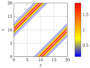
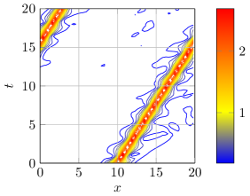
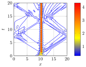
As an example, we set , and . The initial value is set to , which is a snapshot of a solitary wave solution for the case .
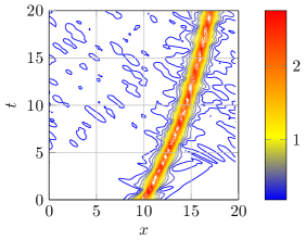
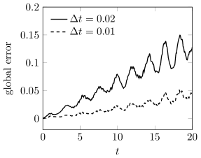
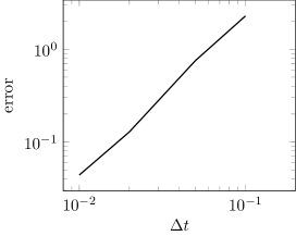
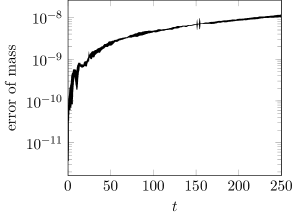
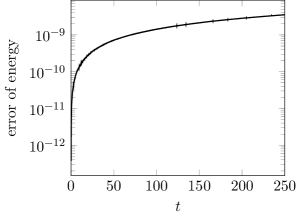
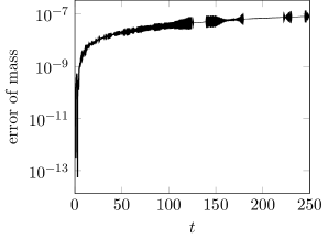
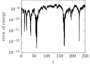
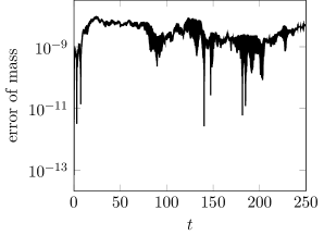
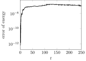
Figs. 1, 2 and 3 show the contour of the absolute value of numerical results for several obtained by the linearly implicit scheme (23) and the nonlinear scheme (47). It is observed that the linearly implicit scheme exhibits qualitatively comparable results to the expensive nonlinear scheme. We note that if gets further small the behaviour is deteriorated as shown in Fig. 4. This figure shows the result for the case and . It is observed that the speed of the wave tends to be slower than that of the reference solution. Let us also check the behaviour in terms of the choice of the time step size in more detail for the case . The results are displayed in Fig. 5. From the left figure, it is observed that the global error becomes small as the time step sizes gets small. Since the scheme is symmetric we expect the second order convergence. From the right figure it seems that the scheme is actually of order two. Figs. 6, 7 and 8 show errors of the discrete mass and energy. For the discrete mass is plotted and for the discrete energy is plotted. Both discrete quantities are well-preserved as expected (note that the tolerance of the linear and nonlinear solvers are set to and the scheme is computed times until ).


4.2. Preservation of the standard energy
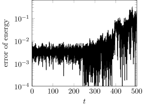
While the discrete mass defined on a single time step is preserved, the discrete energy defined in (28) is not a conserved quantity. We here investigate to what extent remains close to because the value could be a good barometer when we consider the long-time stability. It seems quite challenging to obtain an a priori estimate for the scheme (23), and thus we consider this numerically. Fig. 9 shows the results for the case . It is observed that is bounded by when . However, when exceeds , the error becomes large with strong oscillation, and thus we cannot expect an error bound for for all . With other choices of parameters, qualitatively similar behaviour is observed. These observations indicate that the instability might be caused for a very long-time integration. This could be a drawback of the proposed linearly implicit scheme compared with the nonlinear scheme (47). However, we emphasize that since is easily monitored during the time integration, we could easily detect a sign of the instability.
4.3. Performance of the preconditioning
We here discuss the performance of linear solvers for solving (25).
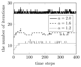
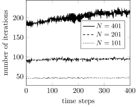
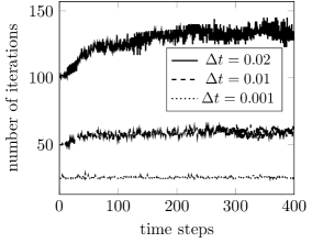
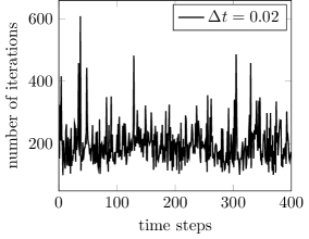
First, we consider solving the original system (25) by the COCG method. Fig. 10 shows the number of iterations required to the convergence for several settings. It is observed that more iterations are required for large , , . In particular, there is a significant gap when we change or . However, we would also like to emphasize that even in the worst case (, and ), the result is much better than that by the Bi-CGSTAB method, which is illustrated in Fig. 11. We thus conclude that when we solve the original system (25) directly, the COCG method seems an appropriate choice. We also note that the COCR method gives comparable results to the COCG method.
Although the COCG method is preferred for solving (25), it is hoped that the convergence behaviour is improved. Thus, we next discuss how the variable transformation and preconditioner proposed in Section 3.4 work. In the following numerical experiments, we consider the case . Table 1 shows the maximum, minimum and average number of iterations of the preconditioned Bi-CGSTAB method for several , where with the time step size and the initial value is set to . The convergence behaviour is outstandingly improved for the case compared with Fig. 11, and furthermore, the results are notable in that for all cases the preconditioned Bi-CGSTAB method requires only three iterations. In this problem setting, the CPU time is shown in Table 2. The computation time seems to be almost proportional to (in the sense that it is a bit worse than , but much better than ). Let us change the time step size to . The results are shown in Table 3. By comparing Table 3 with Table 1, we observe that the convergence behaviour depends on , but the results still remain outstanding. Let us also change the initial value. The results are shown in Table 4, which indicate that the dependency on the shape of solutions is subtle.
| maximum | |||
|---|---|---|---|
| minimum | |||
| average |
| CPU time |
|---|
| maximum | |||
|---|---|---|---|
| minimum | |||
| average |
| maximum | |||
|---|---|---|---|
| minimum | |||
| average |
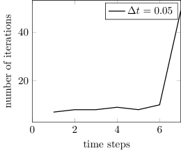
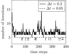
As discussed in Section 3.4, it is also of interest to investigate the behaviour when the COCG method is aggressively applied to the transformed system (58) with the preconditioner (60), since the coefficient matrix in (58) can be seen as a complex symmetric matrix plus a perturbation. Fig. 12 shows the results. From the left figure, it is observed that, when and , the preconditioned COCG method actually work and the results are significantly improved compared with the bottom figure in Fig. 10.
Unfortunately, however, if we use a larger time step size , the preconditioned COCG method requires 50 iterations at the th time step as shown in the right figure of Fig. 12, and the iteration does not converge within iterations at the th time step. This observation indicates that with the step size the influence of the perturbation term is not negligible.
Let us change the initial condition to . This function has a steeper slope. The results are displayed in Fig. 13. It is observed that even if a much larger time step size is employed, the preconditioned COCG method works fine. Conversely, a more gradual initial condition with the time step size was also considered as our preliminary experiments, and it was observed that in this case the preconditioned COCG method did not converge at th time step. These observations indicate that the convergence of the preconditioned COCG method strongly depends on and the shape of the solution (in other words, the influence of ). They make the effect of the perturbation term in (58) significant.
For the problem considered in this paper, it is highly recommended to use the Bi-CGSTAB method with the proposed variable transformation and preconditioner, but it is of interest to understand the behaviour of the preconditioned COCG method, which will be investigated in our future work.

5. Concluding remarks
In this paper, we proposed the linearly implicit scheme (23) for the FNLS equation preserving two invariants: mass and energy. The scheme exhibited qualitatively comparable results to the expensive nonlinear scheme (47). The preconditioning issues were also discussed: the preconditioned Bi-CGSTAB method is a preferable choice.
We note several directions for future work.
-
•
It is hoped that the proposed scheme is used to investigate more challenging problems such as multi-dimensional problems. When we consider the multi-dimensional problems, the computational complexity and preconditioning issues become increasingly important, and thus the discussion on the preconditioning considered for the one-dimensional problem would be helpful.
-
•
The linearly implicit scheme does not preserve , which is defined on a numerical solution of a single time step. The results presented in Fig. 9 should be theoretically investigated in more detail. Note that structure-preserving linearly implicit schemes preserving a certain quantity have also been proposed for other partial differential equations (see, e.g. [5, 23, 24]), and similar behaviour might also have to be reconsidered as well.
-
•
The discussion in Section 4.3 indicates that the COCG/COCR method is applicable to complex but non-symmetric matrices if the non-symmetric term can be regarded as a perturbation in some sense. This behaviour will be investigated theoretically in more detail.
References
- [1] C. Besse, A relaxation scheme for the nonlinear Schrödinger equation, SIAM J. Numer. Anal., 42 (2004), 934–952.
- [2] C. Besse, S. Descombes, G. Dujardin and I. Lacroix-Violet, Energy preserving methods for nonlinear Schrödinger equations, arXiv, 2018.
- [3] E. Celledoni, V. Grimm, R. I. McLachlan, D. I. McLaren, D. O’Neale, B. Owren and G. R. W. Quispel, Preserving energy resp. dissipation in numerical PDEs using the “average vector field” method, J. Comput. Phys., 231 (2012), 6770–6789.
- [4] Y. Cho, G. Hwang, S. Kwon and S. Lee, Well-posedness and ill-posedness for the cubic fractional Schrödinger equations, Discrete Contin. Dyn. Syst., 35 (2015), 2863–2880.
- [5] M. Dahlby and B. Owren, A general framework for deriving integral preserving numerical methods for PDEs, SIAM J. Sci. Comput., 33 (2011), 2318–2340.
- [6] M. Delfour, M. Fortin and G. Payre, Finite-difference solutions of a non-linear Schrödinger equation, J. Comput. Phys., 44 (1981), 277–288.
- [7] S. Duo and Y. Zhang, Mass-conservative Fourier spectral methods for solving the fractional nonlinear Schrödinger equation, Comput. Math. Appl., 71 (2016), 2257–2271.
- [8] E. Faou, Geometric Numerical Integration and Schrödinger Equations, Zurich Lectures in Advanced Mathematics, European Mathematical Society (EMS), Zürich, 2012.
- [9] R. P. Feynman and A. R. Hibbs, Quantum Mechanics and Path Integrals, McGraw-Hill, New York, 1965.
- [10] D. Furihata and T. Matsuo, Discrete Variational Derivative Method: A Structure-Preserving Numerical Method for Partial Differential Equations, Chapman & Hall/CRC, Boca Raton, 2011.
- [11] B. Guo, Y. Han and J. Xin, Existence of the global smooth solution to the period boundary value problem of fractional nonlinear Schrödinger equation, Appl. Math. Comput., 204 (2008), 468–477.
- [12] B. Guo and Z. Huo, Global well-posedness for the fractional nonlinear Schrödinger equation, Comm. Partial Differential Equations, 36 (2011), 247–255.
- [13] X. Guo and M. Xu, Some physical applications of fractional Schrödinger equation, J. Math. Phys., 47 (2006), 082104, 9.
- [14] K. Kirkpatrick, E. Lenzmann and G. Staffilani, On the continuum limit for discrete NLS with long-range lattice interactions, Comm. Math. Phys., 317 (2013), 563–591.
- [15] N. Laskin, Fractional quantum mechanics, Phys. Rev. E, 62 (2000), 3135–3145.
- [16] N. Laskin, Fractional Schrödinger equation, Phys. Rev. E (3), 66 (2002), 056108, 7.
- [17] N. Laskin, Fractional quantum mechanics and Lévy path integrals, Phys. Lett. A, 268 (2000), 298–305.
- [18] M. Li, X.-M. Gu, C. Huang, M. Fei and G. Zhang, A fast linearized conservative finite element method for the strongly coupled nonlinear fractional Schrödinger equations, J. Comput. Phys., 358 (2018), 256–282.
- [19] M. Li, C. Huang and W. Ming, A relaxation-type Galerkin FEM for nonlinear fractional Schrödinger equations, to appear in Numer. Algorithms.
- [20] M. Li, C. Huang and P. Wang, Galerkin finite element method for nonlinear fractional Schrödinger equations, Numer. Algorithms, 74 (2017), 499–525.
- [21] S. Longhi, Fractional Schrödinger equation in optics, Opt. Lett., 40 (2015), 1117.
- [22] T. Matsuo and D. Furihata, Dissipative or conservative finite-difference schemes for complex-valued nonlinear partial differential equations, J. Comput. Phys., 171 (2001), 425–447.
- [23] Y. Miyatake and T. Matsuo, Conservative finite difference schemes for the Degasperis-Procesi equation, J. Comput. Appl. Math., 236 (2012), 3728–3740.
- [24] Y. Miyatake, T. Matsuo and D. Furihata, Invariants-preserving integration of the modified Camassa–Holm equation, Jpn. J. Ind. Appl. Math., 28 (2011), 351–381.
- [25] G. R. W. Quispel and D. I. McLaren, A new class of energy-preserving numerical integration methods, J. Phys. A, 41 (2008), 045206, 7.
- [26] T. Sogabe and S.-L. Zhang, A COCR method for solving complex symmetric linear systems, J. Comput. Appl. Math., 199 (2007), 297–303.
- [27] H. A. van der Vorst, Bi-CGSTAB: a fast and smoothly converging variant of Bi-CG for the solution of nonsymmetric linear systems, SIAM J. Sci. Statist. Comput., 13 (1992), 631–644.
- [28] H. A. van der Vorst and J. B. Melissen, A Petrov–Galerkin type method for solving , where is symmetric complex, IEEE Trans. Mag., 26 (1990), 706–708.
- [29] D. Wang, A. Xiao and W. Yang, A linearly implicit conservative difference scheme for the space fractional coupled nonlinear Schrödinger equations, J. Comput. Phys., 272 (2014), 644–655.
- [30] P. Wang and C. Huang, A conservative linearized difference scheme for the nonlinear fractional Schrödinger equation, Numer. Algorithms, 69 (2015), 625–641.
- [31] P. Wang and C. Huang, An energy conservative difference scheme for the nonlinear fractional Schrödinger equations, J. Comput. Phys., 293 (2015), 238–251.
- [32] P. Wang and C. Huang, Split-step alternating direction implicit difference scheme for the fractional Schrödinger equation in two dimensions, Comput. Math. Appl., 71 (2016), 1114–1128.
- [33] P. Wang and C. Huang, Structure-preserving numerical methods for the fractional Schrödinger equation, Appl. Numer. Math., 129 (2018), 137–158.
- [34] P. Wang, C. Huang and L. Zhao, Point-wise error estimate of a conservative difference scheme for the fractional Schrödinger equation, J. Comput. Appl. Math., 306 (2016), 231–247.
- [35] Y. Zhang, X. Liu, M. R. Belić, W. Zhong, Y. Zhang and M. Xiao, Propagation dynamics of a light beam in a fractional Schrödinger equation, Phys. Rev. Lett., 115.