ZMCintegral: a Package for Multi-Dimensional Monte Carlo Integration on Multi-GPUs

Abstract

We have developed a Python package ZMCintegral for multi-dimensional Monte Carlo integration on multiple Graphics Processing Units(GPUs). The package employs a stratified sampling and heuristic tree search algorithm. We have built three versions of this package: one with Tensorflow and other two with Numba, and both support general user defined functions with a user-friendly interface. We have demonstrated that Tensorflow and Numba help inexperienced scientific researchers to parallelize their programs on multiple GPUs with little work. The precision and speed of our package is compared with that of VEGAS for two typical integrands, a 6-dimensional oscillating function and a 9-dimensional Gaussian function. The results show that the speed of ZMCintegral is comparable to that of the VEGAS with a given precision. For heavy calculations, the algorithm can be scaled on distributed clusters of GPUs.

PROGRAM SUMMARY

Manuscript Title: ZMCintegral: a Package for Multi-Dimensional Monte Carlo Integration on Multi-GPUs
Authors: Hong-Zhong Wu; Jun-Jie Zhang; Long-Gang Pang; Qun Wang
Program Title: ZMCintegral
Journal Reference:
Catalogue identifier:
Licensing provisions: Apache License Version, 2.0(Apache-2.0)
Programming language: Python
Operating system: Linux
Keywords: Monte Carlo integration; Stratified sampling; Heuristic tree search; Tensorflow; Numba; Ray.
Classification: 4.12 Other Numerical Methods
External routines/libraries: Tensorflow; Numba; Ray
Nature of problem: Easy to use python package for Multidimensional-multi-GPUs Monte Carlo integration
Solution method: Stratified sampling and heuristic tree search using multiple GPUs on distributed clusters

1 Introduction

Integrations of high dimensional functions are frequently encountered in computional physics. For example, the total cross sections for particle scatterings in high energy physics[1, 2], and the transport equations over phase space in many body physics[3, 4, 5], etc. These integrations are usually time consuming due to the so called curse of dimensionality[6, 7]; and often, the ill-behaved integrands make the standard quadrature formulae infeasible. Monte Carlo algorithms, with its non-deterministic intrinsic, is particularly useful for higher-dimensional integrals.

The Monte Carlo integration method usually requires large sample points to increase its calculation precision. One of the most popular Monte Carlo algorithms for integration is VEGAS[8], where the methods of importance sampling and adaptive stratified sampling are applied and implemented on CPU with a user-friendly interface. The newly versioned VEGAS, containing an adaptive multi-channel sampling method (Ref. [9]), improves the accuracy for some typical integrals, without introducing much longer evaluation time. However, as the dimensionality increases, the required number of samples increases exponentially to achieve sufficient precision. Therefore, a parallelization of CPUs is needed to handle these large samples. It is proposed in Ref. [10], that VEGAS, with a semi-micro-parallelization method, can be utilized on multi-CPUs to increase speed.

GPUs originally designed for accelerating high-quality computer video games are proved to be very good at single instruction multiple data parallelizations, where simple computation kernels are executed in parallel on thousands of processing elements/threads that a single GPU of a personal computer would have today. gVEGAS [11], which parallelized VEGAS on GPU using CUDA [12, 13], brought $\approx 50$ times performance boost compared to the CPU version. In the same paper [11], a program called BASES [14] which deals with the integration of singular functions is parallelly performed on GPU as gBASES by KEK (The High Energy Accelerator Research Organization in Japan). However, both gVEGAS and gBASES cannot currently run in multi-GPU devices, and no easy-to-use API has been yet released.

Foam [15], another platform for Monte Carlo integration, based on dividing the integration domain into small cells, is also popular but lacks an official release of GPU supported version. Recently, an improved method using Boosted Decision Trees and Generative Deep Neural Networks suggested an advanced importance-sampling algorithm for Monte Carlo integration [16].

In this paper, we propose an easy-to-use python package, ZMCintegral, for multi-dimensional Monte Carlo integration on distributed multi-GPU devices. The source codes and manual can be found in Ref. [17]. It uses both stratified sampling and heuristic tree search algorithm to perform Monte Carlo integration in each cell of the integration domain. Speed and accuracy are both of our concern. It usually takes about a few minutes to finish the evaluation and outputs an integral result with an estimated standard deviation. The algorithm is scalable as its speed is increased with the number of GPUs being used.

Currently, we have built three versions of ZMCintegral on multi-GPUs, one based on Tensorflow eager mode [18][19][20], the other two based on Numba [21]. The Tensorflow version wrapped the difficulties and complexities of multi-GPU parallelization, such as correctly handle the CPU-GPU data transfer, the synchronization, and dealing with the difference between global, local and private memories of GPUs, deeply under beneath Google Tensorflow, which is a python library developed originally for machine learning studies and provides easy-to-use Python function interfaces. We have demonstrated that this is a very good procedure for multi-GPUs parallelization of scientific programs, especially for inexperienced scientific researchers. The other two versions, based on Numba, are different in their parallelizing methods. One uses python Multiprocessing library and focuses on one node computation with multiple GPUs. The other uses Ray [22] and performs the calculation on multiple nodes. The numba versions are highly optimized and flexible at a deep level, which makes high dimensional integration feasible in a reasonable time. All the above features make ZMCintegral an easy-to-use and high performance tool for multi-dimensional integration.

2 The structure of ZMCintegeral

2.1 Stratified sampling and heuristic tree search

In our calculation, the whole integration domain is divided into $k$ ($k$ is an integer) equal sub-domains, with each sub-domain a hypercube of the same volume. Then the integral in each hypercube is calculated using the direct Monte Carlo method, and the integration process is repeated independently by $n_{1}$ times to get $n_{1}$ independent integration values in each sub-domain. For each integration in one sub-domain, the total number of sampled points is $n_{2}^{D}$, where $n_{2}$ is the number of points in each dimension for every sub-domain and $D$ is the dimension of the integration. If the number of sampled points is big enough, each of these $n_{1}$ integration values is a good approximation of the real value for the specific sub-domain. After $n_{1}$ independent integration value for each sub-domain is calculated, the mean and standard deviation of these $n_{1}$ integration values are computed for all $k$ sub-domains. For some of the sub-domains, the standard deviation of $n_{1}$ integration is larger than the threshold value (one hyper-parameter, and can be determined by the mean and standard deviation of the calculated $k$ standard deviations), indicating that the fluctuation is still too large and the integration precision is not sufficient. As a result, these sub-domains need to be recalculated by recursively being split into $k$ new smaller sub-domains.

For example, if the standard deviation in one sub-domain is larger than the threshold value, the integrand in that sub-domain may strongly fluctuate and the mean integration value may not be trusted, suggesting that the integration has to be recalculated with higher accuracy. For those sub-domains whose standard deviations are lower than the threshold value, their mean integration values are accepted as the real values of the sub-domain integration. For those sub-domains whose integrations have to be recalculated, we divide each sub-domain further into $k$ equal sub-sub-domains (depth 2). The same Monte Carlo calculation is applied to these sub-sub-domains to obtain a new list of integration values and corresponding standard deviations. Then a new threshold value is set to filter out those sub-sub-domains that need to be recalculated. This procedure continues until the standard deviations in all sub(-sub-$\cdots$)-domains are lower than the threshold value or the maximal partition depth is reached. Here the partition depth is defined as the total number of layers the integration domain is divided. For example, if the partition depth is 1, the integration domain would only be divided once and sub-domains would not be further divided. Finally the accepted integration values are collected in all sub-domains or sub(-sub-$\cdots$)-domains to obtain the total integration value. At the same time, the standard deviations are collected to obtain the integration error. The algorithm is illustrated in Fig. 1.

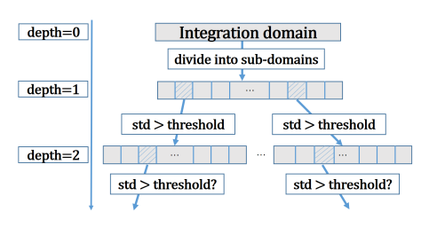
Figure 1: The illustration of the algorithm in ZMCintegral. The integration domain is divided into sub-domains and a threshold value is set to filter out those sub-domains whose integration values are unstable and have to be recalculated. These unstable sub-domains are further divided into sub-sub-domains and the integration in the sub-sub-domains are calculated. The same procedure is continued until the integration values in all sub(-sub-$\cdots$)-domains are accepted or the maximal partition depth is reached.

2.2 Usage of multi-GPUs

One major difficulty to implement multi-dimensional integrations on GPU with the stratified method is the limitation of graphic memory. The reason is that the random numbers generated to calculate the integral occupy a huge memory. The cost of graphic memory increases linearly with the number of sub-domains. To solve this problem, we may apply two methods: the first one is to use multi-GPUs to avoid insufficient memory, where every GPU device only tackles limited sample points. The second one is to modify the way we deal with random numbers generating[23]: instead of producing the random numbers in batch and storing them in the graphic memory for later use, we only produce the random number at the time when using it. For example, in calculating the integral in one sub-domain, we produce the random number and calculate the integral, and then iterate this produce-at-calculation process many times by the number of sample points in the sub-domain. The advantage of the produce-at-calculation method is that it allows a very large number of sub-domains which improves the precision of the integration.

We have three implementations of ZMCintegeral. One uses the functionality of TensorFlow (TensorFlow version) on multi-GPU devices but without improving the treatment of random numbers generating. Hence, when the dimension of the integral is not very high (between 4 and 10) the speed of the integration on multi-GPUs increases significantly; however, when the dimension of the integral is very high (larger than 12), the GPU memory will not be enough. In this case, the method of producing random numbers in real-time becomes more efficient. The other two versions of ZMCintegral, a parallel computing package in python on multi-GPUs, are realized with Numba. The difference between the two numba versions is that one realization with multiprocessing package (Numba-Multiprocessing version) can only be used on one node, and the other with Ray [22] (Numba-Ray version) can be used in distributed clusters. The produce-at-calculation process makes sampling a huge number of points possible so that the integration precision is guaranteed. The speed of two the Numba versions are as fast as the TensorFlow version.

2.3 Parameters

For different integrands with different dimensions, we provide some parameters that can be adjusted by users. The typical hyper-parameters are the number of independent repetitive evaluations for one sub-domain, the threshold value above which the sub-domain has to be recalculated, the maximal depth for tree search, and the number of GPUs that are used for the calculation. Other parameters include the number of sub-domains and the number of sample points in one sub-domain. The product of these two parameters is limited by the computing resources. In the TensorFlow version, it is preferred to increase the number of sample points in one sub-domain, while in the Numba versions, it is preferred to increase the number of sub-domains. The detailed parameters and illustrations can be found in Ref. [17].

3 Results and performance

The performance of ZMCintegral is compared with VEGAS for two typical functions: one is an oscillating function with 6 variables

$$f_{1}=\sin(\sum_{i=1}^{6}x_{i}),$$ (1)

the other is a Gaussian function of 9 variables

$$f_{2}=\frac{1}{\left(\sqrt{2\pi}\sigma\right)^{9}}\exp\left(-\frac{1}{2\sigma^{2}}\sum_{i=1}^{9}x_{i}^{2}\right),$$ (2)

where $\sigma=0.01$ and a high peak is located at $x_{i}=0$ for $i=1,\cdots,9$. The integration domains of $f_{1}$ and $f_{2}$ are chosen to be $\{x_{i}\in[0,10],i=1,\cdots,6\}$ and $\{x_{i}\in[-1,1],i=1,\cdots,9\}$ respectively. As an illustration of the oscillation behavior of $f_{1}$ and the high peak feature of $f_{2}$, we plot the two functions with two variables in Fig. 2.

Figure 2: Schematic plot of sine and Gaussian functions with two variables.

In our numerical experiments, the test platform is kept the same for ZMCintegral and VEGAS. For TensorFlow and Numba-Multiprocessing versions, we test them on one machine that can be treated as a single node. The hardware condition for this node is Intel(R) Xeon(R) CPU E5-2620 v3@2.40GHz CPU with 24 processors + 4 Nvidia Tesla K40m GPUs. What have to be mentioned here is that we only test the VEGAS on this node. For the Numba-Ray version, we have tested it on multiple nodes. The hardware condition for the three nodes are Intel(R) Xeon(R) CPU E5-2620 v3@2.40GHz CPU with 24 processors + 4 Nvidia Tesla K40m GPUs, Intel(R) Xeon(R) CPU E5-2680 V4@2.40GHz CPU with 10 processors + 2 Nvidia Tesla K80 GPUs, and Intel(R) Xeon(R) Silver 4110 CPU@2.10GHz CPU with 10 processors + 1 Nvidia Tesla V100 GPU. The K80 card can be seen as the combination of two K40 cards in physical structure. These three nodes are in a local area network.

3.1 Test on one node

The TensorFlow and Numba-Multiprocessing versions are tested in this section. The test is performed on one node with 4 Nvidia Tesla K40m GPU devices. The calculation results and the total evaluation time is compared with that of VEGAS.

For the integral of $f_{1}$, we use both the TensorFlow and Numba-Multiprocessing versions to carry out the integration and compare the results with VEGAS. The parameters for TensorFlow version are set to the following values: the number of sub-domains in one dimension is $3$, the sample points in one sub-domain in one dimension is $20$, the number of independent repetitive evaluations for one sub-domain is $5$, the maximal depth is $2$, and sub-domains with standard deviations larger than $5\sigma$ will be recalculated. We have sampled totally $20^{6}\times 3^{6}\approx 4.67\times 10^{10}$ points for the 6-dimensional integration. For Numba-Multiprocessing version, the parameters are set to the following values: the number of sub-domains in one dimension is $6$, the sample points in one sub-domain in one dimension is $10$, the number of independent repetitive evaluations for one sub-domain is $5$, the maximal depth is $2$, and sub-domains with standard deviations larger than $5\sigma$ will be recalculated. Threads per block is chosen to be 16 initially, block per grids is calculated via threads per block. The number of sample points is same as the TensorFlow version but with more sub-domains and less sample points in one sub-domain. In VEGAS, the calculation is done on the same machine. We found that in order to obtain the accepted precision, the number of sample points must at least be $10^{9}$, as can be seen in Tab. 1 and Fig. 3. We use three modes in the calculation for VEGAS. One with iteration number set to be $10$ and without discarding operation (normal VEGAS usage), the second with the operation of discarding estimates where the initial several iteration steps are discarded, the last one with both discarding operation and the batch mode [24].

To compare the stability, the total evaluation time and accuracy, we list the averaged results of $10$ independent evaluations in Tab. 1 and in Fig. 3.

Table 1: Results for the integral of $f_{1}$. Each data is the averaged value of $10$ independent evaluations. In the most left column, different versions of the packages are used. ZMC_TF_1K40m means the tensorflow version with 1 K40m being used; and ZMC_numba_2K40m means the Numba-Multiprocessing version with 2 K40m being used. VEGAS_pre_estimate means VEGAS with discarding operation; and VEGAS_batch means the VEGAS discarding operation and the batch mode are being used.

	calculation result	standard deviation	sample points	total time (s)
ZMC_TF_1K40m	-48.96	0.76	$4.67\times 10^{10}$	355.8
ZMC_TF_2K40m	-49.20	1.61	$4.67\times 10^{10}$	187.2
ZMC_TF_3K40m	-49.02	1.36	$4.67\times 10^{10}$	125.9
ZMC_TF_4K40m	-49.05	1.13	$4.67\times 10^{10}$	98.8
ZMC_numba_1K40m	-49.56	1.40	$4.67\times 10^{10}$	313.5
ZMC_numba_2K40m	-49.20	1.15	$4.67\times 10^{10}$	169.4
ZMC_numba_3K40m	-49.58	1.03	$4.67\times 10^{10}$	124.8
ZMC_numba_4K40m	-49.09	0.61	$4.67\times 10^{10}$	96.2
VEGAS	-50.47	2.81	$10^{9}$	10238.5
VEGAS_pre_estimate	-49.96	2.25	$10^{9}$	15647.3
VEGAS_batch	-48.94	1.98	$10^{9}$	3857.2

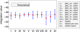
Figure 3: Results for the integral of $f_{1}$. Each data point is the averaged value of $10$ independent evaluations. The data point from left to right: results from the Numba-Multiprocessing version with $4.67\times 10^{6}$ sample points on 1 GPU, 2 GPUs, 3 GPUs, and 4 GPUs, results from the TensorFlow version on 1 GPU, 2 GPUs, 3 GPUs, and 4 GPUs, the results from VEGAS with $10^{9}$ sample points without discarding operation, with $5$ discarding operation, and with $5$ discarding operation and batch mode.

For the integral of $f_{2}$, we only compare the performances of VEGAS and the Numba-Multiprocessing version (the TensorFlow version requires more GPU memory than we can provide). The parameters are: the number of sub-domains in one dimension is $3$, the sample points in one sub-domain in one dimension is $3$, the number of independent repetitive evaluations for one sub-domain is $5$, the maximal depth is $4$, and sub-domains with standard deviations larger than $5\sigma$ will be recalculated. The number of total sample points is $3^{9}\cdot 3^{9}\approx 3.87\times 10^{8}$. In VEGAS, the number of integrand evaluation per iteration is $10^{7}$ such that the evaluation of the integral can be in the lowest cost. The results are shown in 2 and Fig. 4.

Table 2: Results for the integral of $f_{2}$.

	calculation result	standard deviation	sample points	total time (s)
ZMC_numba_1K40m	1.00001	0.00051	$3.87\times 10^{8}$	69.7
ZMC_numba_2K40m	0.99993	0.00048	$3.87\times 10^{8}$	52.8
ZMC_numba_3K40m	1.00016	0.00036	$3.87\times 10^{8}$	45.1
ZMC_numba_4K40m	1.00026	0.00045	$3.87\times 10^{8}$	33.2
VEGAS	0.99987	0.00050	$10^{7}$	510.0

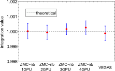
Figure 4: Results for the integral of $f_{2}$. Each data point is the averaged value of $10$ independent evaluations. The data point from left to right: results from the Numba-Multiprocessing version of ZMCintegral on 1 GPU, 2 GPUs, 3 GPUs, and 4 GPUs, the result from VEGAS with 5 steps of discarding operation.

3.2 Test on multiple nodes

The Numba-Ray version supports scalable computations on distributed clusters with Ray [22]. We give the detailed test for this version on one node and multiple nodes. The integrands are choosen to be $f_{1}$ and $f_{2}$ as well.

The parameters for $f_{1}$ is as follows: the number of sub-domains in one dimension is $12$, the sample points in one sub-domain is $10^{4}$, the number of independent repetitive evaluations for one sub-domain is $5$, the maximal depth is $1$. The number of sample points is $12^{6}\times 10^{4}\approx 2.99\times 10^{10}$. Threads per block is choosen to be 32, and we have found very little difference with other values. In our experiments, we have recorded the averaged calculation results, the standard deviation and the total evaluation time. Besides this basic information, we also keep track of the time consumption for tasks allocating and data retrieving between the head node and remote nodes through the network, as well as the evaluation time for single GPU card for one call. The data transfer time between host and device is also recorded. The results are shown in Tab. 3 and in Fig. 5,6,7,8.

Table 3: Integration results for $f_{1}$ with different node configurations. 4 K40m means the calculation is done on one node which uses four K40m. 4 K40m + 2 K80 means the calculation is done using two nodes, one node uses four K40m and the other uses two K80. For evaluations using more than two nodes, the time for Host to Device and Device to Host are monitored seperately for different GPU. For example, 10.7/19.0/20.2 means 10.7 $\mu$s for one K40m per call, 19.0 $\mu$s for one K80 per call and 20.2 $\mu$s for one V100 per call. GPU Calc means the evaluation time per GPU for one call.

	calculation result	standard deviation	total time(s)	allocate(ms)
1K40m	-49.4674	0.8606	298.8	6.5
2K40m	-49.3327	0.4885	122.5	6.7
3K40m	-49.3619	0.5379	57.0	5.9
4K40m	-49.4126	0.7318	35.1	5.9
1V100	-49.3971	0.4845	38.7	3.8
2K80	-49.2317	0.6695	38.9	6.3
4K40m+2K80	-49.4891	0.5896	20.2	7.5
4K40m+2K80+1V100	-49.5273	0.5161	18.4	8.0
	retrieve(ms)	HtoD($\mu$s)	GPU Calc(s)	DtoH(ms)
1K40m	47.0	12.6	2.24	0.87
2K40m	48.9	12.4	2.17	0.81
3K40m	42.6	13.4	2.03	0.90
4K40m	48.8	10.1	1.69	0.62
1V100	45.7	16.3	0.46	0.76
2K80	59.5	15.9	1.83	0.83
4K40m+2K80	761.4	10.5/13.1	1.71/1.82	0.68/0.61
4K40m+2K80+1V100	760.7	10.7/19.0/20.2	1.70/1.86/0.45	0.73/0.68/0.77

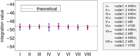
Figure 5: Integration results for $f_{1}$ with different node configurations. Each data point is the averaged value of $10$ independent evaluations. The data point from left to right corresponds to: one node with 4 K40m, one node with 3 K40m, one node with 2 K40m, one node with 1 K40m, one node with 2 K80, one node with 1 V100, two nodes with 4 K40m + 2 K80, three nodes with 4 K40m +2 K80 +1 V100.

Figure 6: Time consumption for different number of GPUs on one node. The left panel shows that when less GPUs are used, the evaluation time per GPU for one call is increasing. This small time deivation will add up to a significant time difference for the total evaluation time, as can be seen in the right panel. The right panel shows that when less GPUs are used, the total evaluation time is not linearly increasing. This non-linearity suggests that more GPUs should be used on one node.

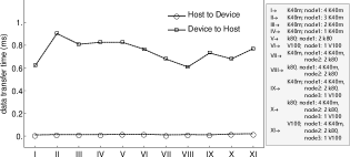
Figure 7: Data transfer time between GPU (device) and CPU (host) with different node configurations. The data point from left to right corresponds to: monitor of each K40m per call when one node with 4 K40m, 3 K40m, 2 K40m or 1 K40m is used, monitor of each K80 per call when one node with 2 K80 is used, monitor of each V100 per call when one node with 1 V100 is used, monitor of each K40m and K80 per call when two nodes with 4 K40m + 2 K80 are used, monitor of each K40m, K80 and V100 per call when three nodes with 4 K40m +2 K80 +1 V100 are used.

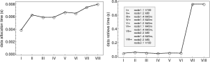
Figure 8: Data allocation and retrieve time from head node to remote nodes with different node configurations. The left panel shows the data allocation time from head to remote nodes via internet connection. It can be seen that more time is needed when more nodes are being involved. The right panel shows the data retrieve time from remote nodes to head node. The “jump” for the last two configurations suggests that when more nodes are used the retrieve time is increased.

For the Gaussian type integration, we test the performance for 9 dimensional integration of $f_{2}$. The parameters are: the number of sub-domains in one dimension is $3$, the sample points in one sub-domain is $10^{4}$, the number of independent repetitive evaluations for one sub-domain is $5$, the maximal depth is $4$, and sub-domains with standard deviations larger than $4\sigma$ will be recalculated. The number of sample points is $3^{9}\times 10^{4}\approx 1.97\times 10^{8}$. The test for the Gaussian type of 12 dimensions is also performed. The results are in Tab. 4 and Fig. 9.

Table 4: Performance on 9-D and 12-D Gaussian integrals. 4 K40m_9D means one node with four K40m are used for 9-D integration and similar for the rest.

	calculation result	standard deviation	total time(s)	allocate(ms)
4K40m_9D	0.99989	0.00059	8.2	0.8
2K80_9D	1.00015	0.00065	9.0	1.2
1V100_9D	1.00035	0.00064	4.8	0.9
1V100_12D	1.00002	0.00079	47.6	1.7
	retrieve(ms)	HtoD(us)	GPU Calc(s)	DtoH(ms)
4K40m_9D	3.9	10.0	0.36	0.50
2K80_9D	4.4	12.1	0.37	0.58
1V100_9D	3.8	15.8	0.16	0.66
1V100_12D	6.9	15.7	0.73	0.72

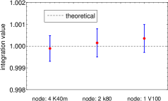
Figure 9: Results for the integral of $f_{2}$ with different node configurations. Each data point is the average value of $10$ independent evaluations. The data point from left to right: 4 K40m as one node, 2 K80 as one node, and V100 as one node.

3.3 Analysis of the results

Under a similar precision, ZMCintegral is much faster in speed than VEGAS in our experiments. We can see in Tab. 1 that for 6 dimensional integration, with the number of sample points being $46$ times larger than that of VEGAS, ZMCintegral is still 10-150 times faster than VEGAS. For the 9 dimensional integration, as is shown in Tab. 2, when the number of sample points is $38$ times larger than that of VEGAS, the speed of ZMCintegral is still 7-15 times faster.

In the test of multiple nodes, we can see that the integration speed is increased when more GPUs (more than 4) are used, as is shown in Tab. 3. From Fig. 6, it is suggested that even on one node more GPUs should be used. The data transfer time between host to device is mainly dominated by the GPU cards. As can be seen from Fig. 7, for different configurations of nodes, the time for HtoD (host to device) and DtoH (device to host) almost kept unchanged.

While VEGAS is more efficient to put sample points in integration domains where the integrand fluctuates dramatically, the GPU backend ZMCintegral with stratified sampling method can put sample points in each sub-domain whose number is comparable to the number of points been put into the emphasized regions of VEGAS. Meanwhile, the use of the heuristic tree search algorithm assures more sample points in sub-domains with more fluctuations. Furthermore, ZMCintegral has an appealing feature: the computation is scalable and its speed is increased with the increasing number of GPUs in usage. While VEGAS often needs a discarding operation process to ensure the reliability of the final result, ZMCintegral only needs an appropriate value of the maximal depth (usually between 2 and 4). In ZMCintegral, we indeed see the effect of the heuristic tree search which yields a more precise result than without the tree search.

A straight forward application of the two Numba version (Numba-Multiprocessing and Numba-Ray) of ZMCintegral is the calculation of the global polarization in heavy ion collisions. There we encounter an oscillating 10-dimensional integration involving three momenta of the two incoming and outgoing particles, where the incoming particles are wave-packets centered at $\mathbf{p}_{A}$ and $\mathbf{p}_{B}$ and the outgoing particles are plane waves with momenta $\mathbf{p}_{1}$ and $\mathbf{p}_{2}$. With proper conservation laws the integration really involves $p_{1,x},p_{1,y},p_{1,z},p_{2,x},p_{2,y},p_{2,z},k_{A,y},k_{A,z},k_{A,y}^{\prime}$ and $k_{A,z}^{\prime}$, where $\mathbf{k}_{A}$ and $\mathbf{k}_{A}^{\prime}$ are the quantum fluctuations about $\mathbf{p}_{A}$. The difficulty for this massive (containing several thousands terms) 10-dimensional integration mainly comes from two aspects. On the one hand, a sufficient number of sample points are required to cover all domains so that the oscillating details should not be smeared out. To be safe, we need around $15^{10}\approx 5.77\times 10^{11}$ sample points, which is almost impossible for normal CPU algorithm. On the other hand, the complexity of the integrand requires a very flexible interface that all the condition checking, pattern matchings and special functions can be easily realized. This we have done with Numba language. The two Numba version of ZMCintegral, with full support of the Numpy and Math packages, is a convenient choice.

4 Conclusion and Discussion

We propose a multi-GPU backend package for Monte Carlo integration using stratified sampling and heuristic tree search algorithm. The package has good performance for integration in large dimensions. As can be seen in our examples, the package is able to control both the time consumption and the accuracy, and it is tens to hundreds times as fast as the traditional CPU based VEGAS. ZMCintegral is really of great help for high dimensional integrations in large scale scientific computation in terms of shortening the period of computing time from months to days.

Instead of manipulating GPU with CUDA directly in C++, we choose the state-of-art multi-GPU parallelization libraries Tensorflow and Numba to build ZMCintegral. Both Tensorflow and Numba are professional and widely used in the community and are easy to use with Python for non-experts.

Though ZMCintegral is able to handle integrations in dimensions up to 16 and even higher, we should also keep in mind its limitation for very high dimensions, for example, above 20. The difficulty lies in the sampling. It was reported by Pan in MIT China submit [25], that we are not even able to deal with $2^{80}$ numbers with all computational resources in the world within a year. So a general Monte Carlo integration based on large scale sampling for very high dimensions has a ceiling, in this case we may need other “renormalization” algorithms to reduce the dimension.

References

-
[1]
M. E. Peskin, D. V. Schroeder,
An Introduction to
quantum field theory, Addison-Wesley, Reading, USA, 1995.
URL http://www.slac.stanford.edu/~mpeskin/QFT.html - [2] J. jie Zhang, R. hong Fang, Q. Wang, X.-N. Wang, A microscopic description for polarization in particle scatteringsarXiv:http://arxiv.org/abs/1904.09152v1.
- [3] S. R. De Groot, Relativistic Kinetic Theory. Principles and Applications, 1980.
- [4] Z. Xu, C. Greiner, Thermalization of gluons in ultrarelativistic heavy ion collisions by including three-body interactions in a parton cascade, Physical Review C 71 (6). doi:10.1103/physrevc.71.064901.
- [5] J.-W. Chen, Y.-F. Liu, Y.-K. Song, Q. Wang, Shear and bulk viscosities of a weakly coupled quark gluon plasma with finite chemical potential and temperature: Leading-log results, Physical Review D 87 (3). doi:10.1103/physrevd.87.036002.
-
[6]
R. E. Bellman,
Dynamic
Programming, PRINCETON UNIV PR, 1957.
URL https://www.ebook.de/de/product/34448612/richard_e_bellman_dynamic_programming.html -
[7]
R. Bellman,
Dynamic
Programming, Dover Publications Inc., 2003.
URL https://www.ebook.de/de/product/3396699/richard_bellman_dynamic_programming.html -
[8]
G. P. Lepage,
A
new algorithm for adaptive multidimensional integration, Journal of
Computational Physics 27 (2) (1978) 192 – 203.
doi:https://doi.org/10.1016/0021-9991(78)90004-9.
URL http://www.sciencedirect.com/science/article/pii/0021999178900049 -
[9]
T. Ohl,
Vegas
revisited: Adaptive monte carlo integration beyond factorization, Computer
Physics Communications 120 (1) (1999) 13 – 19.
doi:https://doi.org/10.1016/S0010-4655(99)00209-X.
URL http://www.sciencedirect.com/science/article/pii/S001046559900209X -
[10]
R. Kreckel,
Parallelization
of adaptive mc integrators, Computer Physics Communications 106 (3) (1997)
258 – 266.
doi:https://doi.org/10.1016/S0010-4655(97)00099-4.
URL http://www.sciencedirect.com/science/article/pii/S0010465597000994 -
[11]
J. Kanzaki, Monte carlo
integration on gpu, The European Physical Journal C 71 (2) (2011) 1559.
doi:10.1140/epjc/s10052-011-1559-8.
URL https://doi.org/10.1140/epjc/s10052-011-1559-8 - [12] I. Buck, T. Purcell, A Toolkit for Computation on GPUs, 2004.
- [13] J. Nickolls, W. J. Dally, The gpu computing era, IEEE Micro 30 (2) (2010) 56–69. doi:10.1109/MM.2010.41.
-
[14]
S. Kawabata,
A
new version of the multi-dimensional integration and event generation package
bases/spring, Computer Physics Communications 88 (2) (1995) 309 – 326.
doi:https://doi.org/10.1016/0010-4655(95)00028-E.
URL http://www.sciencedirect.com/science/article/pii/001046559500028E -
[15]
S. Jadach,
Foam:
A general-purpose cellular monte carlo event generator, Computer Physics
Communications 152 (1) (2003) 55 – 100.
doi:https://doi.org/10.1016/S0010-4655(02)00755-5.
URL http://www.sciencedirect.com/science/article/pii/S0010465502007555 - [16] J. Bendavid, Efficient monte carlo integration using boosted decision trees and generative deep neural networks.
- [17] Location of zmcintegral package, https://github.com/Letianwu/ZMCintegral.git.
- [18] M. Abadi, A. Agarwal, P. Barham, E. Brevdo, Z. Chen, C. Citro, G. Corrado, A. Davis, J. Dean, M. Devin, S. Ghemawat, I. Goodfellow, A. Harp, G. Irving, M. Isard, Y. Jia, L. Kaiser, M. Kudlur, J. Levenberg, X. Zheng, Tensorflow : Large-scale machine learning on heterogeneous distributed systems (01 2015).
-
[19]
M. Abadi, P. Barham, J. Chen, Z. Chen, A. Davis, J. Dean, M. Devin,
S. Ghemawat, G. Irving, M. Isard, M. Kudlur, J. Levenberg, R. Monga,
S. Moore, D. G. Murray, B. Steiner, P. Tucker, V. Vasudevan, P. Warden,
M. Wicke, Y. Yu, X. Zheng,
Tensorflow:
A system for large-scale machine learning, in: 12th USENIX Symposium on
Operating Systems Design and Implementation (OSDI 16), USENIX
Association, Savannah, GA, 2016, pp. 265–283.
URL https://www.usenix.org/conference/osdi16/technical-sessions/presentation/abadi - [20] Tensorflow eager mode, https://www.tensorflow.org/guide/eager.
- [21] S. Kwan Lam, A. Pitrou, S. Seibert, Numba: a llvm-based python jit compiler, 2015, pp. 1–6. doi:10.1145/2833157.2833162.
-
[22]
P. Moritz, R. Nishihara, S. Wang, A. Tumanov, R. Liaw, E. Liang, M. Elibol,
Z. Yang, W. Paul, M. I. Jordan, I. Stoica,
Ray: A
distributed framework for emerging AI applications, in: 13th USENIX
Symposium on Operating Systems Design and Implementation (OSDI 18),
USENIX Association, Carlsbad, CA, 2018, pp. 561–577.
URL https://www.usenix.org/conference/osdi18/presentation/moritz - [23] I. Deák, Uniform random number generators for parallel computers, Parallel Computing 15 (1990) 155–164. doi:10.1016/0167-8191(90)90039-C.
- [24] Vegas tutorial, https://www.vegas.readthedocs.io/en/latest/tutorial.html.
- [25] P. Jian-wei, The quantum computing: Present and future, MIT China Submit (2018).