Filamentous Active Matter:
Band Formation, Bending, Buckling, and Defects

Motor proteins drive persistent motion and self-organisation of cytoskeletal filaments. However, state-of-the-art microscopy techniques and continuum modelling approaches focus on large length and time scales. Here, we perform component-based computer simulations of polar filaments and molecular motors linking microscopic interactions and activity to self-organisation and dynamics from the two-filament level up to the mesoscopic domain level. Dynamic filament crosslinking and sliding, and excluded-volume interactions promote formation of bundles at small densities, and of active polar nematics at high densities. A buckling-type instability sets the size of polar domains and the density of topological defects. We predict a universal scaling of the active diffusion coefficient and the domain size with activity, and its dependence on parameters like motor concentration and filament persistence length. Our results provide a microscopic understanding of cytoplasmic streaming in cells and help to develop design strategies for novel engineered active materials.

Introduction

The key structural and active element operating biological cells is their cytoskeleton, which to a large extent is composed by polar filaments dynamically interconnected by passive and active crosslinkers  (?, ?). The cytoskeleton provides mechanical stability to cells, acts as dynamic force-generating element, and serves as a track network for active intracellular transport  (?, ?). Moreover, internal motion of the cytoplasm, which can be generated by the dynamics of the cytoskeleton, secures nutrient availability and the distribution of organelles  (?). Fundamental knowledge about the relationship between cytoskeleton structure and dynamics is therefore necessary to obtain a deeper understanding of cellular function and dysfunction in vivo, and for design and synthesis of active-gel materials, e.g., artificial cells  (?, ?). In dilute suspensions of freely diffusing filaments and motors, the filaments self-organise into large-scale aster-like structures and vortices  (?, ?). In contrast, in dense suspensions of filaments and motors at an oil-water interface, pioneering experiments  (?, ?, ?, ?) have revealed exciting non-equilibrium behaviours, such as persistent spontaneous flows and turbulence. In particular, the formation of topological defects has been shown to be a clear signature of active nematics  (?).

Component-based computer simulations have greatly advanced the field of passive colloidal systems in the past, as well as the emerging field of active materials in recent times. In the latter, non-equilibrium, energy-consuming processes drive the system, which lead to very rich collective behavior  (?, ?, ?, ?). For example, ensembles of self-propelled rod-like particles form novel liquid-crystalline steady states  (?, ?, ?, ?, ?). Single self-propelled, semiflexible filaments form spirals, while multiple filaments cluster and their dynamics changes from jamming to active turbulence with increasing Peclet number  (?). At high densities, where the equilibrium phase of the corresponding passive system is nematic, continuum models predict spontaneous flows and turbulence  (?, ?, ?, ?, ?, ?). Computational modelling has also been used to study cellular processes connected to cytoskeletal dynamics, like mitosis and contractility  (?, ?).

Important and challenging questions for filament-motor systems include the identification of the roles of hydrodynamic interactions, filament flexibility, and motor and crosslinker properties. While existing continuum models indicate that hydrodynamic interactions are an essential element for the formation of defect structures  (?, ?), this is in contrast with results obtained with models of apolar active elipsoids  (?) and self-propelled filaments  (?), and experiments of vibrated granular rods  (?). In these systems, defect formation and complex dynamics have been observed in the absence of hydrodynamics. Flexibility of the filaments must also be relevant, because in simulations of mixtures of stiff rods and motors topological defects have not been observed  (?, ?, ?). Finally, passive cross-linkers have been demonstrated to be key to change the behavior of a filament-motor mixture from extensile to contractile  (?).

In this paper, we study the emergent structures and persistent dynamics in mixtures of semiflexible filaments and molecular motors using Langevin Dynamics simulations. Our microscopic, filament-based modelling approach for dilute and concentrated systems bridges length scales from nanometer-sized molecular motors to micrometer-long, semiflexible filaments, and time scales from tens of microseconds for single-motor steps to seconds for cytoplasmic streaming  (?, ?). Our two-dimensional simulations correspond to experimental studies for filament-motor suspensions at oil-water interfaces  (?). Our calculations show that the average motor-induced force on antiparallel filaments is a robust measure for the activity in the system. The generated active stresses induce a buckling-type instability in initially nematic filament systems. At steady state, complex flow patterns emerge that lead to continuous creation and annihilation of topological defects, and to active Brownian particle-like filament diffusion at long time scales.

Our simulations are based on a model of semiflexible filaments of contour length $L$ and persistence length $\ell_{\mathrm{p}}$ in two dimensions. Filaments consist of $n_{\mathrm{s}}$ beads of diameter $\sigma$ connected by stiff harmonic springs with rest length $a_{0}=L/(n_{\mathrm{s}}-1)$ where $a_{0}=\sigma$. The filament area fraction $\phi=n_{\mathrm{f}}n_{\mathrm{s}}\pi\sigma^{2}/4L_{\mathrm{box}}^{2}$ is varied by changing the number of filaments, $n_{\mathrm{f}}$, or the box size $L_{\mathrm{box}}$. Molecular motors are modelled by harmonic springs with rest length $r_{0}$ and spring constant $k_{\mathrm{m}}$, and attach to neighbouring filaments with rate $\Gamma_{\mathrm{att}}$. Motors walk in the direction of the filament polarity with step length $a_{0}$. The step rate is proportional to the probability $p_{\mathrm{m}}^{0}$ to move a motor arm, which sets the bare motor velocity $v_{0}=a_{0}p_{\mathrm{m}}^{0}/\Delta t$, where $\Delta t$ is the motor time step. Motors detach when they reach the end of a filament, when they encounter a motor already bound, or when their length exceeds a threshold $r_{\mathrm{off}}$. In the following we use the reduced quantities: filament aspect ratio $\tilde{L}=L/\sigma$, motor-to-filament ratio $\tilde{n}_{\mathrm{m}}=n_{\mathrm{m}}/n_{\mathrm{f}}$, persistence length $\tilde{\ell}_{\mathrm{p}}={\ell}_{\mathrm{p}}/L$, motor spring constant $\tilde{k}_{\mathrm{m}}=k_{\mathrm{m}}r_{0}^{2}/k_{\mathrm{B}}T$ ($k_{\mathrm{B}}T$ is the thermal energy), filament friction $\tilde{\gamma}=\gamma/k_{\mathrm{m}}\delta t$ ($\delta t$ is the simulation time step), box size $\tilde{L}_{\mathrm{box}}=L_{\mathrm{box}}/L$, and time $\tilde{t}=tD_{0}/L^{2}$, with $D_{0}$ the single passive-filament translational diffusion coefficient. For details see Methods.

Results

Activity drives the formation of polar domains

The microscopic origin of filament motion is the active and dynamic crosslinking of filaments by molecular motors. Because filaments are intrinsically polar, the resulting parallel forces depend on the relative orientation of connected filaments. If these two filaments are polar-aligned, and two consecutive motor steps occur on the two different filaments, the motors induce no net filament motion, see Fig. 1a. However, if the filaments are anti-aligned, the motors get stretched and net filament motion results, see Fig. 1b. The $n_{\mathrm{m}}$ motors are classified as $n_{\mathrm{m}}^{\mathrm{p}}$ ’parallel motors’ that connect parallel filaments in the interior of domains, and ${n_{\mathrm{m}}^{\mathrm{ap}}}$ ’anti-parallel motors’ that dynamically crosslink and slide filaments at the interfaces between oppositely oriented domains relative to each other.

An initially disordered nematic suspension of filaments transforms into an ”active polar nematic” when molecular motors are added. The motor-induced sliding forces first lead to a rapid sorting of filaments into narrow polar bands with antiparallel alignment at the domain boundaries, see Fig. 1c. In time, these polar bands coarsen. When the activity is large enough, a buckling instability leads to disordered configurations of polar domains with topological defects, see Fig. 1d. If the activity is too small or the filaments are too stiff, the steady state consists of stable parallel bands, see fig. SI 1. Video 1 illustrates the polarity-sorting process in more detail. Video 2 shows the entire dynamical evolution from the initial nematic state to the stationary state.

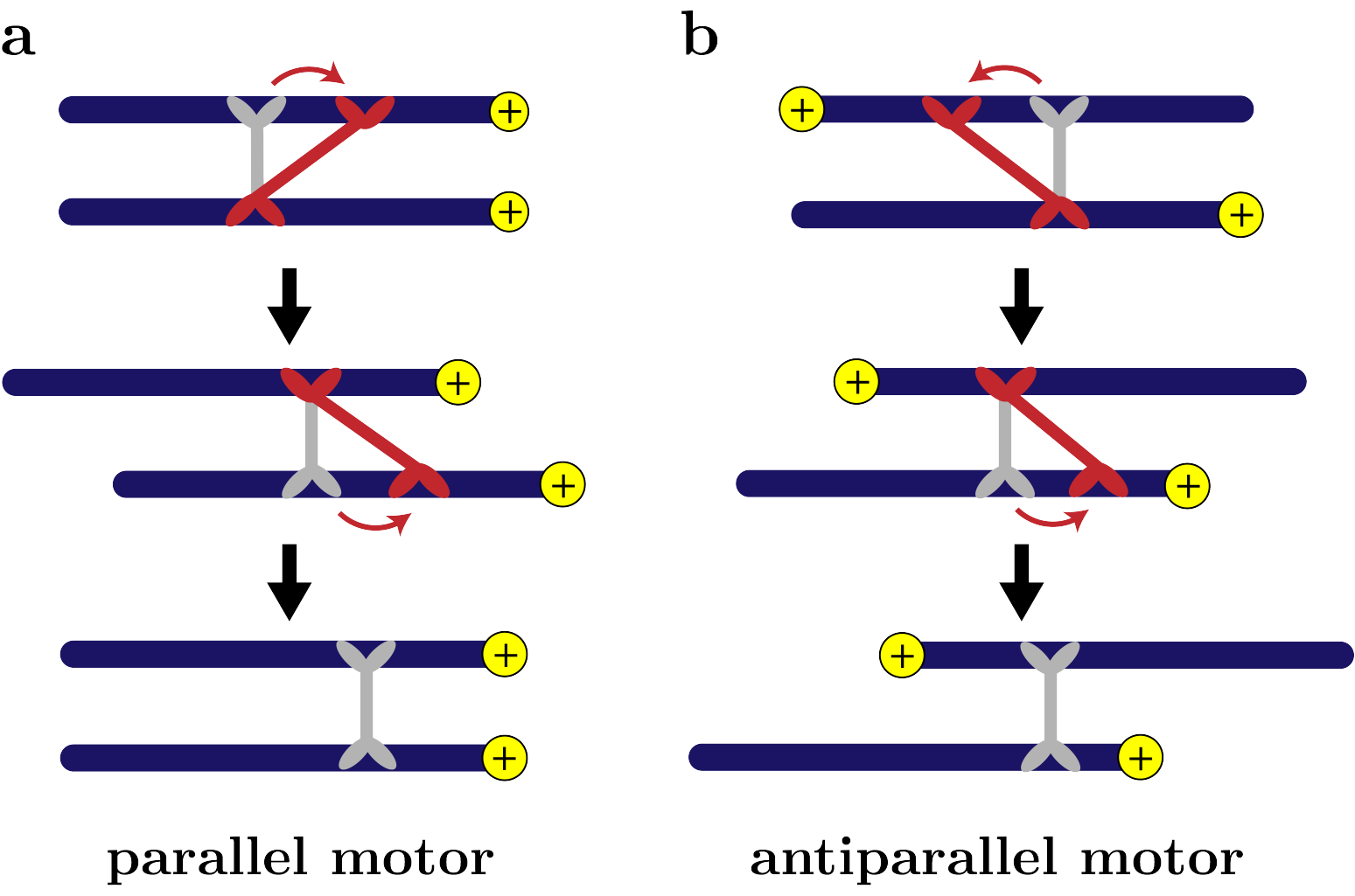
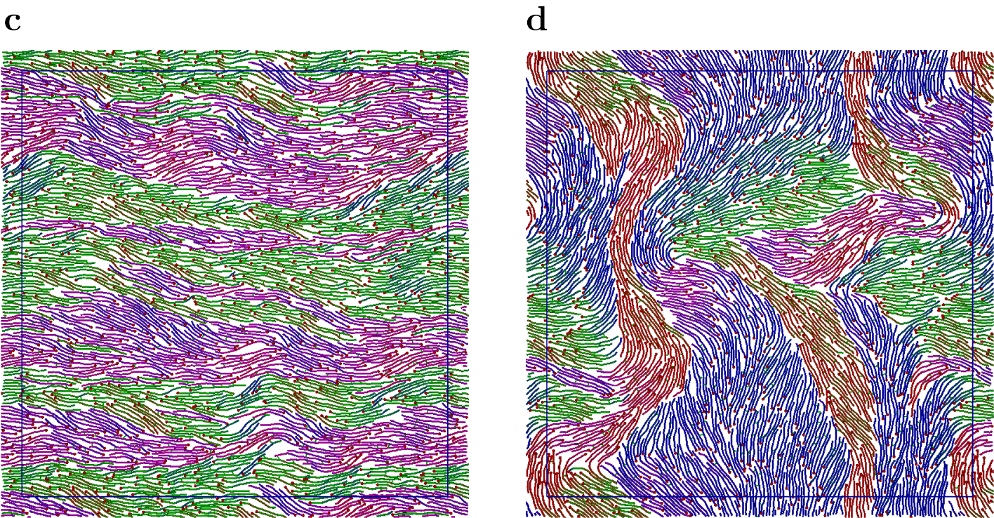
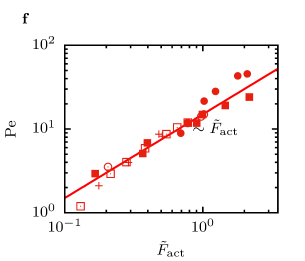
${\tilde{\ell}_{\mathrm{p}}}$ $\tilde{k}_{\mathrm{m}}$ $\tilde{\gamma}$ $p_{\mathrm{m}}^{0}$ $\tilde{n}_{\mathrm{m}}$ $\blacksquare$ 1-7 12.5 4 1 0.89 $\odot$ 2.4 6.25-50 1-8 1 0.89 $\bullet$ 2.4 12.5 0.4-400 1 0.89 $\Box$ 2.4 12.5 4 0.01-1 0.89 $+$ 3.4 12.5 4 1 0.5-3.6

Fig. 1: Self-organised structures and dynamics of motor-filament mixtures driven by sliding of antiparallel filaments.
                                                                                                                                                                                                     a,b Sketches of two consecutive motor steps when filaments are oriented a parallel b antiparallel. The initially relaxed grey motor steps towards the filament polar end, it relaxes and it makes a second step on the other filament and relaxes again. This results in net filament motion only for antiparallel motors. c,d Simulation snapshots for an initially disordered nematic system. The thin black box indicates the central simulation cell. c short-time band formation and d long-time disordered structures. Filament colours indicate their orientation, illustrated by the colour axis. e Number of antiparallel motors as a function of the persistence length $\ell_{\mathrm{p}}$, and the bare motor velocity, measured by $p_{\mathrm{m}}^{0}$. f Peclet number as a function of the active force $\tilde{F}_{\mathrm{act}}$ in Eq. (1). The table shows the parameter combinations used in (e,f). In all cases ($\phi,\tilde{L}$)=(0.66, 20).

Steady-state filament dynamics emerges from a complex interplay between various filament and motor properties. For example, the number of antiparallel motors is an important factor driving the filament dynamics, as well as the suspension structure. Figure 1e shows that the fraction of antiparallel motors increases with decreasing filament persistence length $\ell_{\mathrm{p}}$ and with increasing bare motor velocity. As we will show later, a shorter persistence length leads to smaller domains and overall larger interface length, such that more antiparallel motors can be accommodated. Similarly, larger motor velocities lead to a higher activity and to smaller domains. We quantify the activity by the total motor force in the system as

$$\tilde{F}_{\mathrm{act}}={n_{\mathrm{m}}^{\mathrm{ap}}}\tilde{k}_{\mathrm{m}}\left(\frac{{r_{\mathrm{m}}}}{r_{\mathrm{0}}}-1\right)$$ (1)

with the average relative extension ${r_{\mathrm{m}}}/r_{\mathrm{0}}-1$ of the antiparallel motors. In steady state, the motor force is balanced by an effective friction force with friction coefficient $\gamma_{\mathrm{eff}}\propto D_{0}^{-1}$; the parallel filament velocity $v_{\parallel}$ is defined as ${v_{\parallel}=\lim_{\tau\to 0}\langle-{\bf p}(t)\cdot\left({\bf r}(t+\tau)-{\bf r}(t)\right)/\tau\rangle_{t}}$, where ${\bf r}(t)$ and ${\bf p}(t)$ are the position and the unit tangent vector of the filament center, respectively, and $\tau$ is the lag time, see fig. SI 2. The parallel velocity and thus the Peclet number $\mathrm{Pe}=v_{\parallel}L/D_{0}$ increases linearly with the activity (total active force) in the system, see Fig. 1 f. Note that the active force $\tilde{F}_{\mathrm{act}}$ indirectly depends on $\ell_{\mathrm{p}}$ and $\tilde{n}_{\mathrm{m}}$, thus the same magnitude can be achieved by different combinations of parameters.

Single-filament motion and active diffusion

To characterise single filament motion in the active steady states, we calculate the filament orientational autocorrelation functions and filament center-of-mass mean squared displacements (MSD). For non-zero $\tilde{n}_{\mathrm{m}}$ and intermediate times, the filaments follow essentially straight trajectories. Their ballistic motion, with $\textrm{MSD}\propto v_{\parallel}^{2}\tau^{2}$, is a signature of this active persistent motion. At long times, the filaments lose their initial orientation due to active rotational motion, and the MSD becomes again linear with time, characterised by a plateau in Fig. 2a, with an active diffusion coefficient $D_{\rm act}$ that increases with increasing $\tilde{n}_{\mathrm{m}}$. The filament orientational autocorrelation functions decay exponentially with an active decay time $\tau_{\mathrm{R}}$, which also depends on $n_{\mathrm{m}}$. The active rotation time $\tau_{\mathrm{R}}$ is shown in Fig. 2b both as a function of $n_{\mathrm{m}}$ and $F_{\mathrm{act}}$. For small $n_{\mathrm{m}}$, increasing the number of motors first leads to a faster motion but at $\tilde{n}_{\mathrm{m}}\approx 1.5$ the motion becomes slower again because the number of antiparallel motors per filament ${n_{\mathrm{m}}^{\mathrm{ap}}}$ does not increase anymore (see fig. SI 3); the excess motors increase the crosslinking density inside the polar domains which reduces the filament velocity. The active rotation time $\tau_{\mathrm{R}}$ decreases with increasing $F_{\mathrm{act}}$ (${n_{\mathrm{m}}^{\mathrm{ap}}}$) with a power law, $\tau_{\mathrm{R}}\propto F_{\mathrm{act}}^{\nicefrac{{-3}}{{2}}}$. The active diffusion coefficient, parallel velocity, and rotational correlation times for many different parameter variations are related by $D_{\rm act}\propto v_{\parallel}^{2}\tau_{\mathrm{R}}$, see Fig. 2c, consistent with the theory of active Brownian motion  (?).

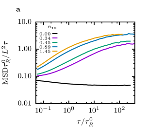
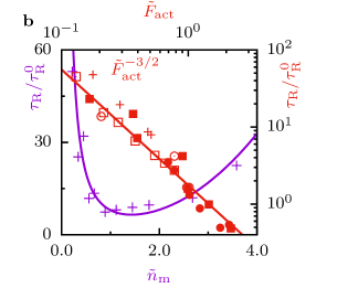
Fig. 2: Single-filament motion and active diffusion for various propulsion forces.
                                                                                                                                          a Filament mean squared displacement divided by the lag time for different motor concentrations $\tilde{n}_{\mathrm{m}}$. The lag time $\tau$ is normalised with the passive single-filament rotation time $\tau_{\mathrm{R}}^{0}$, and the MSD with the filament length $L^{2}$. The parameters are ($\phi,\tilde{\ell}_{\mathrm{p}},\tilde{L}$)=(0.66, 3.4, 20). b Normalised active rotation times $\tau_{\mathrm{R}}$ as function of $n_{\mathrm{m}}$ and $\tilde{F}_{\mathrm{act}}$. Solid lines are a guide to the eye, parameters as in Fig. 1f with ($\phi,\tilde{L}$)=(0.66, 20). c Normalised active diffusion constants obtained from MSD-curves as a function of the filament measured $v_{\parallel}^{2}\tau_{\mathrm{R}}$, parameters as in Fig. 1f with ($\phi,\tilde{L}$)=(0.66, 20).

Buckling polar bands

The strength of the active force does not only determine the average filament velocity, but also structure, size, and stability of the domains. Polar bands are stable for weak active forces and large persistence lengths, whereas they become unstable and buckle at a particular wavelength $\lambda$ for sufficiently large active forces. The time evolution of the motor-filament mixture in Fig. 3a-c shows polarity-sorted bands, progressive bending and breaking of bands, see also Video 3. The wavelength $\lambda$ at the instability displays a square-root dependence on the filament persistence length $\ell_{\mathrm{p}}$ (see fig. 3d). The assumption that the active force in all these systems evolves independent of the persistence length (see Fig. SI 4) suggests an Euler buckling-type instability with buckling force $F_{\mathrm{b}}\propto E/\lambda^{2}$. Here $E\propto\ell_{\mathrm{p}}$ is the (effective) elastic modulus (Frank constant)  (?). Together with $F_{\mathrm{b}}\sim{n_{\mathrm{m}}^{\mathrm{ap}}}$ this provides the scaling $\lambda^{2}\propto\ell_{\mathrm{p}}/{n_{\mathrm{m}}^{\mathrm{ap}}}$. This scaling was also found in wet active nematics   (?, ?, ?, ?, ?, ?) with the same argument of balancing active stress and nematic elasticity. The investigation of the stability of the system with simulations at various combinations of $\tilde{n}_{\mathrm{m}}$ and $\tilde{\ell}_{\mathrm{p}}$ allows us to determine the phase diagram shown in Fig. 3e. Here the stability limit of the polarity-sorted bands increases with increasing persistence length, which nicely agrees with the predicted linear dependence of the buckling force on $\tilde{\ell}_{\mathrm{p}}$.

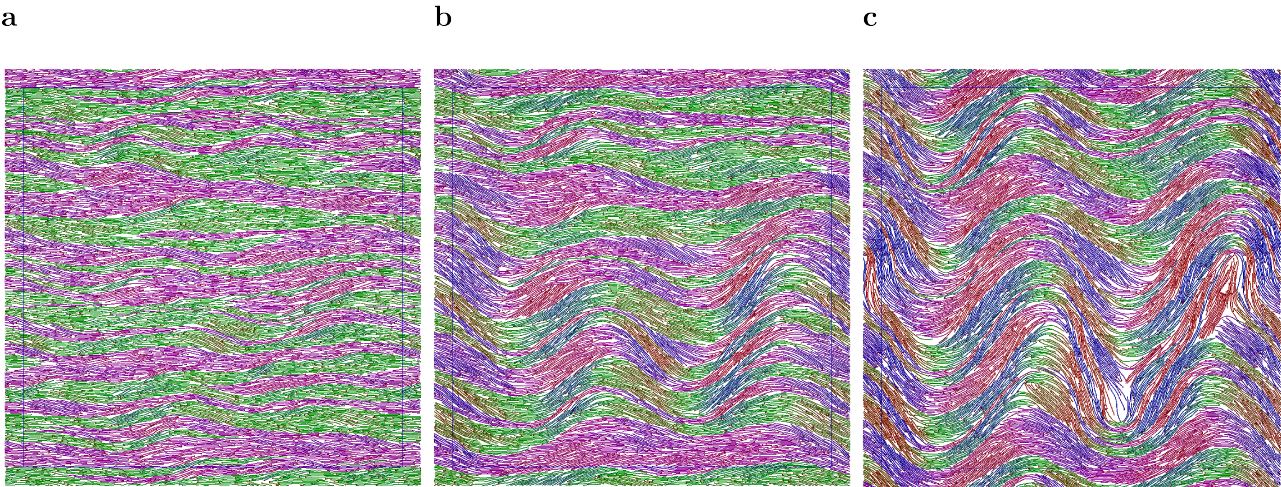
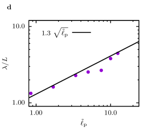
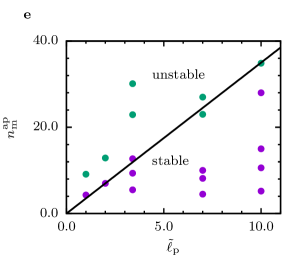
Fig. 3: Onset of domain formation: Euler-like buckling instability of polar bands.
                                                                                                                                          a-c Snapshots of the time evolution of a initially nematic system with $(\phi,\tilde{\ell}_{\mathrm{p}},\tilde{L})=(0.66,10,40)$, for $t/\tau_{\mathrm{R}}^{0}=0.1,0.2,0.3$ respectively. d Wavelength of the instability of polar-sorted bands as a function for varying persistence length and $(\phi,\tilde{L})=(0.66,40)$. e Stability phase diagram for various active forces and persistence lengths with paramaters $(\phi,\tilde{L})=(0.66,20)$. The solid line separates different phases and indicates the values of the buckling force.

Intradomain dynamics

Our component-based model also provides detailed microscopic information about the filament dynamics within the polar domains. We studied configurations with a stable number of bands, an example of which is shown in Fig. 4a. The corresponding velocity profiles are calculated for various values of the active force by changing $n_{\mathrm{m}}$, see Fig. 4b. The average band velocity increases linearly with ${n_{\mathrm{m}}^{\mathrm{ap}}}$, in agreement with the results in Fig. 1f. The total length of the interface, $L_{\mathrm{inter}}\simeq n_{\mathrm{b}}\mathrm{b}L_{\mathrm{box}}$, varies by changing the number of bands, or by enlarging the box size. The band velocity is roughly independent of the persistence length, see Fig. 4c, which indicates that the interfacial structure is not dramatically affected by the filament flexibility.

       
   

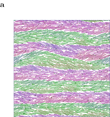
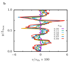
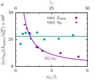
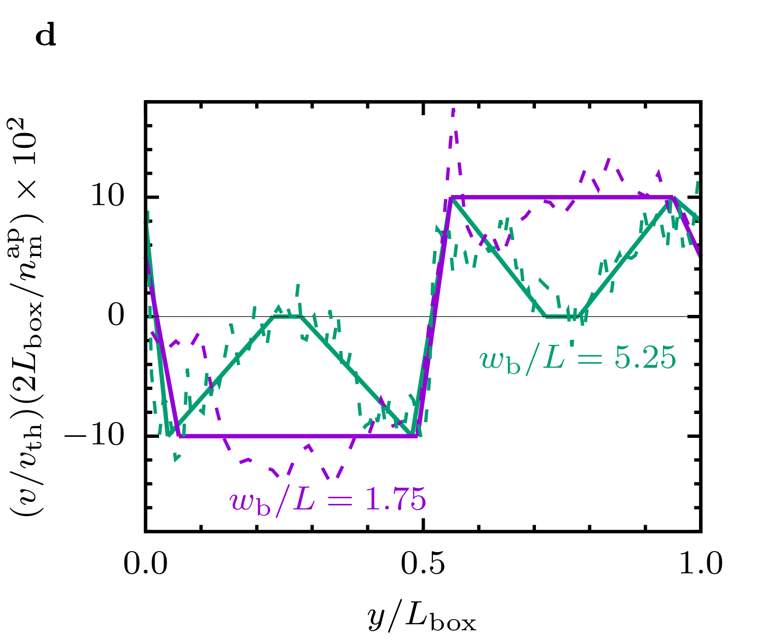
Fig. 4: Intra-band filament dynamics for narrow and wide bands at steady state.
                                                                                                                                          a Snapshots for a system with parallel bands for $(\phi,\tilde{\ell}_{\mathrm{p}},n_{\mathrm{b}},\tilde{n}_{\mathrm{m}})=(0.66,20,8,0.12)$. b Velocity profiles for various $\tilde{n}_{\mathrm{m}}$. $(\phi,\tilde{\ell}_{\mathrm{p}},n_{\mathrm{b}})=(0.66,20,8)$ c Normalised averaged band velocities as a function of the band width $w_{\mathrm{b}}$ and the persistence length $\ell_{\mathrm{p}}$ of the filaments for $(n_{\mathrm{b}},\tilde{n}_{\mathrm{m}})=(6,0.45)$. The antiparallel motor density is ${n_{\mathrm{m}}^{\mathrm{ap}}}/L_{\mathrm{inter}}$ where $L_{\mathrm{inter}}=n_{\mathrm{b}}L_{\mathrm{b}}$ is the total length of the interface in the system. d Normalised velocity profiles for two band widths. Dashed lines are simulation results and solid lines are guides to the eye.

The results shown above demonstrate that the force applied by the antiparallel motors at the interfaces generates the motion of the bands. The parallel motors connecting filaments within the bands transmit this force in the perpendicular direction, but the friction with the embedding medium strongly reduces the velocity in the center of the bands for wide bands. From velocity profile for the wide bands, see Fig.4 d, we estimate the velocity decay length to be between half and two filament lengths. This is confirmed by an explicit calculation of the velocity correlation length from the velocity correlation function as outlined in fig. SI 5, fig. SI 6 and fig. SI 7. Moreover, the velocity correlation length is rather insensitive to a change in activity as was also found in Ref.  (?), but does depend on the persistence length, see fig. SI 8.

For narrow bands, the velocity profiles of the two interfaces overlap, resulting in plug flow-type velocity profiles, as shown in Fig. 4d. Note that in most cases the orientation of the filaments at the interface has a well-defined inclination angle ($15^{\circ}-25^{\circ}$), see for example Fig. 4a or Fig. 1c. Thus motors between antiparallel filaments can only attach close to the filament ends imposing a pushing force from the rear end. Closer to the center of a band, the filaments are oriented parallel to the interface.

Dynamics of topological defects

The system of polar filaments and motor proteins shares features with both active nematics, and polar active fluids, although it is clearly distinguishable from both of them. As for active nematics, anti-parallel motion at the interfaces drives the dynamics; as for polar active fluids, polar order emerges within the domains. However the characteristic topological defects that appear in polar active fluids, $+1$ or $-1$ defects  (?), are never observed here. Instead, the defect structures in the dynamic disordered phase are $\nicefrac{{+1}}{{2}}$ and $\nicefrac{{-1}}{{2}}$ topological defects, as shown in Fig. 5. A defect pair is formed when a polar band buckles by extensional forces, such that the convex side forms a $\nicefrac{{+1}}{{2}}$ defect, while the concave side forms a $\nicefrac{{-1}}{{2}}$ defect, see Fig. 5a. Importantly, these are not the standard defects of active nematics, because the three domains which meet at a $\nicefrac{{-1}}{{2}}$ defect display polar order, which implies that there can be active forces where domains with anti-parallel polar order meet. In particular, our polar filament model gives rise to two types of $\nicefrac{{-1}}{{2}}$ defects with different orientations of the polar domains around the defect core. One has $C_{1}$ symmetry, the other $C_{3}$ symmetry, see Figs. 5b and c. Note that for the $C_{1}$-defect in Fig. 5b, there are additional (unmarked) boundaries between anti-parallel domains in the lower left and right corners where the motion is originated.

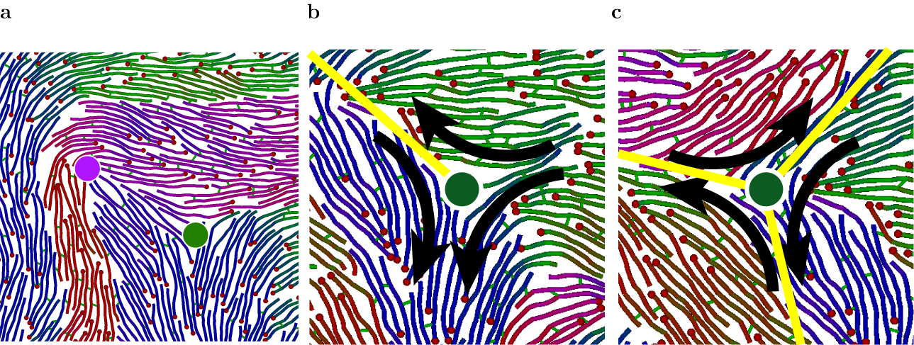
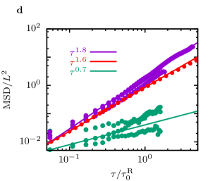
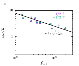
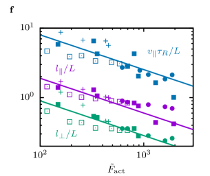
Fig. 5: Densities and mean squared displacements of topological +1/2 and -1/2 defects.
                                                                                                                                          a Snapshot of a pair of $\nicefrac{{-1}}{{2}}$ (green) and a $\nicefrac{{+1}}{{2}}$ (magenta) defects. b Polar and nematic order near a $\nicefrac{{-1}}{{2}}$ defect with $C_{1}$ symmetry. c Polar and nematic order near a $\nicefrac{{-1}}{{2}}$ defect with $C_{3}$ symmetry. In (a), (b) and (c), filament colors indicate the polar angle of filament orientation. In (b) and (c), the yellow lines indicate boundaries between polar domains. d MSD of the filament center-of-mass (red), $\nicefrac{{-1}}{{2}}$ defects (green) and of $\nicefrac{{+1}}{{2}}$ defects (magenta). e Average distance between defects as a function of the active force. f Estimation of the domain size with three different approaches. Solid lines show the $1/\sqrt{F_{\mathrm{act}}}$ dependence, and symbols simulations with data sets from the table in Fig. 1 with $(\phi,\tilde{L})=(0.66,20)$.

The topological defects are calculated following Refs.  (?, ?) and show super-diffusive motion of the $\nicefrac{{+1}}{{2}}$ defects, and sub-diffusive motion of the $\nicefrac{{-1}}{{2}}$ defects as follows from the defects MSDs in Fig. 5d and illustrated in Video 4. The annihilation of two defects is shown in Video 5. However, we do not find any differences in the dynamic behaviour of the two types of $\nicefrac{{-1}}{{2}}$ defects. The defect density depends linearly on the activity, which is reflected by the inverse square root dependence of the distance $l_{\mathrm{def}}$ between the defects on the force as shown in Fig. 5e. A similar scaling is found for a related characteristic length scale in the system, the domain size, shown in Fig. 5f. The exponential decay of the parallel and perpendicular spatial orientational correlation functions $\widehat{\Omega}_{\mathrm{\parallel}}(r)$ and $\widehat{\Omega}_{\mathrm{\perp}}(r)$ (see fig. SI 9) provides the correlation lengths $l_{\perp}$ and $l_{\parallel}$, which are estimations for width and length of the domains. An independent estimate is $v_{\parallel}\tau_{\mathrm{R}}$  (?), which is proportional to the distance that a filament moves along the domain boundary, before changing direction. Note that both $\tau_{\mathrm{R}}$ and $v_{\parallel}$ are averaged values over a distribution of faster (antiparallel) and slower (parallel) filaments. Although these three lengths provide different quantitative estimations of the domain size, their scaling is consistent with an inverse square-root dependence on the activity.

Universality of domain-size scaling and active diffusion

In passive lyotropic liquid crystalline systems particle density and shape determine both structural and dynamical properties. For active systems, however, the active force provides an additional control parameter. Figure  6a-d shows simulation snapshots for various filament densities and different $\tilde{n}_{\mathrm{m}}$, chosen such that ${n_{\mathrm{m}}^{\mathrm{ap}}}/n_{\mathrm{f}}$ is comparable so that the systems have similar active force densities. We observe a gradual change from small local bundles held together by motors at low densities, to a dense disordered nematic dominated by excluded-volume interactions similarly as in experiments  (?). Although the structures observed are very different, the (parallel) velocities still show a unique linear scaling with the force density $v_{\parallel}\propto{\rm Pe}\propto{F_{\mathrm{act}}/n_{\mathrm{f}}}$, see Fig. 6e. However, the active rotation times shown in Fig. 6f show a significant dependence on the density, especially for small densities and low activities, where the active rotation time is similar to the passive one. Nevertheless, for large activities and for large densities again a unique scaling behaviour $\tau_{\mathrm{R}}\sim(\tilde{F}/n_{\mathrm{f}})^{\nicefrac{{-3}}{{2}}}$ is observed, see also Fig. 2b. Therefore, at large densities or large activities, the active diffusion coefficient $D_{\mathrm{act}}\sim v_{\parallel}^{2}\tau_{\mathrm{R}}$ and domain size $v_{\parallel}\tau_{\mathrm{R}}$ show a universal scaling, see Fig. 6g. The chosen scaling variables ($F_{\mathrm{act}}/n_{\mathrm{f}}$, $\tau_{\mathrm{R}}/\tau_{\mathrm{R}}^{0}$ and $v_{\parallel}L/D_{0}$) are independent of the filament length, as indicated by of three simulations for filaments twice as long as all our other simulations.

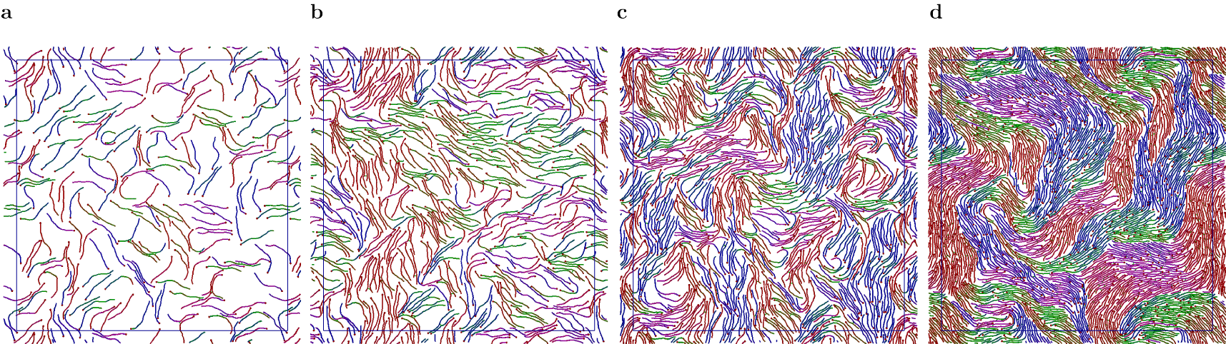
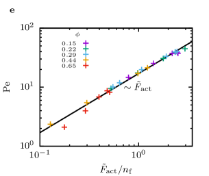
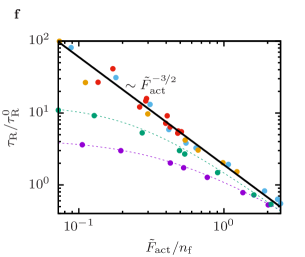
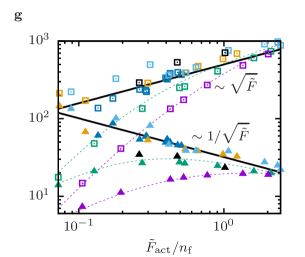
Fig. 6: Filament density-dependent structure formation and single-filament dynamics.
                                                                                                                                          a-d Snapshots for systems at various densities, $\phi=(0.15,0.29,0.44,0.66)$, where $n_{\mathrm{m}}$ is varied to result in similar $n_{\mathrm{m}}^{\mathrm{ap}}/n_{\mathrm{f}}\approx 0.165$. e-g Dimensionless observables as a function of the active force for different area fractions. Symbols correspond to simulation data, dashed lines are to guide the eye and full lines indicate limiting powerlaws at large densities: e Peclet number, f active rotation time, g active diffusion coefficient $v_{\parallel}^{2}\tau_{\mathrm{R}}$ (open squares), and domain size $v_{\parallel}\tau_{\mathrm{R}}$ (solid up-triangles). Colored labels in (e) refer to densities in (e, f, g). Black symbols in (g) correspond to simulations with longer filaments with $(\phi,\tilde{\ell}_{\mathrm{p}},\tilde{L})=(40,0.66,1.7)$.

Discussion

Our simulations of semiflexible polar filaments crosslinked by molecular motors generate macroscopic active domains and defect formation in the absence of hydrodynamic interactions. The simulations reveal a novel structure, an ’active polar nematic’, which consists of nematically arranged polar domains. Essential results of the simulations are that activity manifests at domain boundaries, not inside domains, and that new types of topological defects appear, which are distinguished by the two possible arrangements of polar orientation at a three-fold junction. An initially nematic arrangement of filaments is unstable and is found to evolve via polarity sorting, band formation, and buckling into a stationary but highly dynamic polar-domain structure with persistent defect formation and annihilation. We find universal scaling of active filament diffusion and of domain sizes with the active force determined by the number of antiparallel motors and their extension. Our model can readily be extended to three-dimensional systems, to study the effects of stiff and (semi)flexible confinements, as well as of models with an increased level of complexity like the inclusion of passive crosslinkers or hydrodynamic interactions.

Materials and Methods

Suspensions of $n_{\mathrm{f}}$ semiflexible filaments and $n_{\mathrm{m}}$ motors are studied using Langevin dynamics  (?) in two dimensions with periodic boundary conditions. Semiflexible filaments of length $L$ are modelled as discrete chains of $n_{\mathrm{s}}$ beads of mass $m$ with position vectors ${\mathbf{r}}_{q}^{i}$ where $q=\{1....n_{\mathrm{f}}\}$ and $i=\{1....n_{\mathrm{s}}\}$. The $n_{\mathrm{s}}$ beads define $n_{\mathrm{s}}-1$ segments of length $a_{0}=L/(n_{\mathrm{s}}-1)$ with unit tangent vectors $\hat{{\mathbf{t}}}_{q}^{i}=(\mathbf{r}_{q}^{i+1}-\mathbf{r}_{q}^{i})/|\mathbf{r}_{q}^{i+1}-\mathbf{r}_{q}^{i}|$. The beads are connected by harmonic bonds with equilibrium length $a_{0}$ and spring constant $kr_{\mathrm{0}}^{2}/\mathrm{k}_{\mathrm{B}}T=250$. A bending potential $V_{\mathrm{b}}=\kappa(1-\hat{{\mathbf{t}}}_{q}^{i}\cdot\hat{{\mathbf{t}}}_{q}^{i+1})/a_{0}$ gives rise to a tangent vector correlation function $\left<{\bf t}(0)\cdot{\bf t}(s)\right>=\exp[-s/\ell_{\mathrm{p}}]=\exp[-(d-1)\mathrm{k}_{\mathrm{B}}Ts/2\kappa]$ with dimensionality $d$ and arclength $s$ along the contour, such that the bare persistence length is $\ell_{\mathrm{p}}/L=2\kappa/L\mathrm{k}_{\mathrm{B}}T$  (?). Non-bonded inter and intramolecular excluded volume and attractive interactions are described by a Lennard Jones potential $V_{LJ}=\varepsilon[(\sigma/r)^{12}-2(\sigma/r)^{6}]$ where $r$ denotes the inter or intra molecular bead-bead separation, $\varepsilon$ the interaction strength, $\sigma$ the interaction diameter, i.e. the beads are not overlapping) and $r_{c}=3\sigma$ the potential cut-off radius. In all our simulations $k_{\mathrm{B}}T/\varepsilon=10$, i.e. attractions between filaments are negligible. These parameters lead to an effective Barker-Henderson diameter  (?) which is 14% less than that for a system with a purely repulsive WCA potential at $\varepsilon/k_{\mathrm{B}}T=1.0$ and 4% less than the WCA potential with $\varepsilon/k_{\mathrm{B}}T=0.1$. The filament beads also act as binding sites for molecular motors. These are modelled as harmonic springs $V_{\mathrm{m}}=k_{\mathrm{m}}(r-r_{\mathrm{0}})^{2}/2$ with spring constant $k_{\mathrm{m}}$ and equilibrium length $r_{\mathrm{0}}=\sigma$ that walk on the filaments  (?, ?, ?, ?). Note that here the discretisation length $a_{0}$ directly sets the motor step size. When the separation between two empty sites on nearby filaments is smaller than $r_{\mathrm{att}}$ a free (unbound) motor can bind at a rate $(p_{\mathrm{att}}/\delta t)\ (n_{\mathrm{m}}^{\mathrm{f}}/n_{\mathrm{m}})$ where $n_{\mathrm{m}}^{\mathrm{f}}$ is the number of free motors and $p_{\mathrm{att}}=1$ in all simulations. When bound, the $n_{\mathrm{m}}^{\mathrm{b}}$ motors walk in the direction of filament polarity (from segment $1\rightarrow n_{\mathrm{s}}$) in discrete steps of size $a_{0}$ at a rate $\Gamma=p_{\mathrm{m}}^{0}/\Delta t\ \exp{(-\beta\Delta E)}$. Here $p_{\mathrm{m}}^{0}$ is the probability for an attempted step of a motor attached to two filaments, $\Delta t$ the motor time-step and $\Delta E$ the energy difference before and after the motor has stepped. Motors detach only when one leg reaches the end of the filament or when the motor is stretched beyond a length $r_{\mathrm{off}}=3.25\ r_{0}$. After detaching, the free motors form a bath with homogeneous concentration $n_{\mathrm{m}}^{\mathrm{f}}/L_{\mathrm{box}}^{2}$ where $L_{\mathrm{box}}$ is the box size. The Langevin equation of motion for each bead $i$ on filament $q$,

$$m\frac{\mathrm{d}^{2}{\bf r}_{q}^{i}}{\mathrm{d}t^{2}}={\bf F}_{q}^{i}-\gamma\frac{\mathrm{d}{\bf r}_{q}^{i}}{\mathrm{d}t}+{\bf R}_{q}^{i},$$ (2)

is integrated with a time step $\delta t$ using the integrator proposed in Ref.  (?). In order to satisfy the fluctuation-dissipation theorem the random forces are Gaussian distributed with mean zero and variance ${2\mathrm{k}_{\mathrm{B}}T\gamma\delta(t-t^{\prime})}$. The integration time step $\delta t$ and friction $\gamma$, were chosen such that $\delta t/m=0.005$ and $\gamma\delta t/m\geq 0.005$. For these parameters the (passive) center-of-mass motion of a single filament is diffusive for center-of-mass displacements larger than a fraction of the length of a filament, i.e., for center-of-mass diffusion the dynamics is essentially overdamped. Note that the simulation time increases linearly with the friction constant. Simulations typically contain 900 filaments of 21 beads and up to 3200 motors.

The coupling of filaments by molecular motors leads to sliding and binding forces that depend on the relative orientation of the filaments, see Fig. 1a,b, where antiparallel motors (coupling two antiparallel filaments) exert larger forces than parallel motors (coupling two parallel filaments). Moreover, the activity induced by dimeric motors (one motorarm is grafted) tetrameric motors (both motor arms move simultaneously) is larger  (?). The motor model here is a hybrid of the two, both motor arms can move with equal probability but only one at a time.

Rotational diffusion is measured through the filament orientation correlation function, where the orientation is defined as the eigenvector corresponding to the largest eigenvalue of the moment of inertia tensor.

Supplementary Materials

Movie S1. Dynamics of polarity sorting and coarsening of polar bands from the initial disordered nematic state.

Movie S2. Steady state dynamics of polar domains with repeated creation and annihilation of defect pairs.

Movie S3. Dynamics of the elastic instability. Formation and buckling of polar bands leads to the emergence of the disordered phase.

Movie S4. Defect dynamics. Extensile motion of a $\pm$$\nicefrac{{1}}{{2}}$ defect pair.

Movie S5. Annihilation of a $\nicefrac{{+1}}{{2}}$ (blue) and $\nicefrac{{-1}}{{2}}$ defect (purple).

Fig. S1. Time sequence of filament self-organisation.

Fig. S2. Normalised parallel velocity $v_{\parallel}/v_{\mathrm{th}}$.

Fig. S3. Time evolution of the number of antiparallel motors.

Fig. S4. The number of antiparallel motors as a function of the total number of motors.

Fig. S5. Segment orientational correlation functions.

Fig. S6. Filament velocity correlation functions for three motor densities.

Fig. S7. Time scale renormalization for active motion.

Fig. S8. Amplitude and velocity decorrelation length of the velocity correlation function function.

Fig. S9. Dependence of the velocity correlation length on the persistence length.

Acknowledgements: The authors thank Roland G Winkler for helpful conversations.
Author Contributions: GV, TA and GG conceived the research. GV wrote all simulation codes, performed simulations and analysed the data. All authors wrote the manuscript.
Competing Interests: The authors declare that they have no competing financial interests.
Data and materials availability: Additional data and materials are available online.

References

- 1. S. Köhler, V. Schaller, A. R. Bausch, Structure formation in active networks. Nat. Mater. 10, 462–468 (2011).
- 2. C. Veigel, C. F. Schmidt, Moving into the cell: single-molecule studies of molecular motors in complex environments. Nat. Rev. 12, 163 (2011).
- 3. D. A. Fletcher, R. D. Mullins, Cell mechanics and the cytoskeleton. Nature 463, 485–492 (2010).
- 4. C. Lin, M. Schuster, S. C. Guimaraes, P. Ashwin, M. Schrader, J. Metz, C. Hacker, S. J. Gurr, G. Steinberg, Active diffusion and microtubule-based transport oppose myosin forces to position organelles in cells. Nat. Commun. 7, 11814 (2016).
- 5. W. Lu, M. Winding, M. Lakonishok, J. Wildonger, V. I. Gelfand, Microtubule–microtubule sliding by kinesin-1 is essential for normal cytoplasmic streaming in drosophila oocytes. Proc. Natl. Acad. Sci. U.S.A. 113, 4985 (2016).
- 6. F.-C. Tsai, B. Stuhrmann, G. H. Koenderink, Encapsulation of active cytoskeletal protein networks in cell-sized liposomes. Langmuir 27, 10061–10071 (2011).
- 7. D. Needleman, Z. Dogic, Active matter at the interface between materials science and cell biology. Nat. Rev. Mater. 2, 1–14 (2017).
- 8. R. Urrutia, M. A. McNiven, J. P. Albansei, D. B. Murphy, B. Kachar, Purified kinesin promotes vesicle motility and induces active sliding between microtubules in vitro. Proc. Natl. Acad. Sci. U.S.A. 88, 6701–6705 (1991).
- 9. F. J. Nedelec, T. Surrey, A. C. Maggs, S. Leibler, Self-organization of microtubules andmotors. Nature 389, 305 (1997).
- 10. T. Sanchez, D. T. N. Chen, S. J. DeCamp, M. Heymann, Z. Dogic, Spontaneous motion in hierarchically assembled active matter. Nature 491, 431 (2012).
- 11. F. C. Keber, E. Loiseau, T. Sanchez, S. J. DeCamp, L. Giomi, M. J. Bowick, M. C. Marchetti, Z. Dogic, A. R. Bausch, Topology and dynamics of active nematic vesicles. Science 345, 1135 (2014).
- 12. G. Henkin, S. J. DeCamp, D. T. N. Chen, T. Sanchez, Z. Dogic, Tunable dynamics of microtubule-based active isotropic gels. Phil. Trans. R. Soc. A 372, 1 (2014).
- 13. P. Guillamat, J. Ignés-Mullol, F. Sagués, Taming active turbulence with patterned soft interfaces. Nat. Commun. 8, 564 (2017).
- 14. S. Ramaswamy, The mechanics and statistics of active matter. Annu. Rev. Condens. Matter Phys. 1, 323–345 (2010).
- 15. M. Marchetti, J. F. Joanny, S. Ramaswamy, T. B. Liverpool, J. Prost, M. Rao, R. A. Simha, Hydrodynamics of soft active matter. Rev. Mod. Phys. 85, 1143 (2013).
- 16. S. E. Spagnolie, ed., Theory of active suspensions (Springer Science+Business Media, 2015), chap. 9, p. 319.
- 17. J. Elgeti, R. G. Winkler, G. Gompper, Physics of microswimmers—single particle motion and collective behavior: a review. Rep. Prog. Phys. 78, 056601 (2015).
- 18. H. H. Wensink, H. Löwen, Emergent states in dense systems of active rods: from swarming to turbulence. J. Phys.: Condens. Matter 24, 464130 (2012).
- 19. M. Abkenar, K. Marx, T. Auth, G. Gompper, Collective behavior of penetrable self-propelled rods in two dimensions. Phys. Rev. E 88, 062314–11 (2013).
- 20. L. Giomi, M. J. Bowick, P. Mishra, R. Sknepnek, M. C. Marchetti, Defect dynamics in active nematics. Phil. Trans. R. Soc. A 372, 20130365 (2014).
- 21. M. Sheetz, J. Spudich, Movement of myosin- coated fluorescent beads on actin cables in vitro. Nature 303, 31-35 (1983).
- 22. T. Yanagida, M. Nakase, K. Nishiyama, F. Oosawa, Direct observation of motion of single f-actin filaments in the presence of myosin. Nature 307, 58–60 (1984).
- 23. Ö. Duman, R. E. Isele-Holder, J. Elgeti, G. Gompper, Collective dynamics of self-propelled semiflexible filaments. Soft Matter 14, 4483-4494 (2018).
- 24. L. Giomi, Geometry and topology of turbulence in active nematics. Phys. Rev. X 5, 031003 (2015).
- 25. S. P. Thampi, R. Golestanian, J. M. Yeomans, Velocity correlations in an active nematic. Phys. Rev. Lett. 111, 118101 (2013).
- 26. S. P. Thampi, R. Golestanian, J. M. Yeomans, Vorticity, defects and correlations in active turbulence. Phil. Trans. R. Soc. A 372, 20130366 (2014).
- 27. A. Doostmohammadi, M. F. Adamer, S. P. Thampi, J. M. Yeomans, Stabilization of active matter by flow-vortex lattices and defect ordering. Nat. Commun. 7, 10557 (2016).
- 28. E. J. Hemingway, P. Mishra, M. C. Marchetti, S. M. Fielding, Correlation lengths in hydrodynamic models of active nematics. Soft Matter 12, 7943-7952 (2016).
- 29. F. N. Eric Karsenti, T. Surrey, Modelling microtubule patterns. Nat. Cell Biol. 8, 1204–1211 (2006).
- 30. D. Z. E. Nazockdast, A. Rahimian, M. Shelley, A fast platform for simulating semi-flexible fiber suspensions applied to cell mechanics. J. Comp. Phys. 329, 173–209 (2017).
- 31. X. qing Shi, Y. qiang Ma, Topological structure dynamics revealing collective evolution in active nematics. Nat. Commun. 4, 3013 (2013).
- 32. V. Narayan, S. Ramaswamy, N. Menon, Long-lived giant number fluctuations in a swarming granular nematic. Science 317, 105–108 (2007).
- 33. R. Blackwell, O. Sweezy-Schindler, C. Baldwin, L. E. Hough, M. A. Glaser, M. D. Betterton, Microscopic origins of anisotropic active stress in motor-driven nematic liquid crystals. Soft Matter (2016).
- 34. A. Ravichandran, G. A. Vliegenthart, G. Saggiorato, T. Auth, G. Gompper, Enhanced dynamics of confined cytoskeletal filaments driven by asymmetric motors. Biophys. J. 113, 1121–1132 (2017).
- 35. A. Ravichandran, O. Duman, M. Hoore, G. Saggiorato, G. A. Vliegenthart, T. Auth, G. Gompper, Chronology of motor-mediated microtubule streaming. eLife 8, e39694 (2019).
- 36. J. M. Belmonte, M. Leptin, F. Nédélec, A theory that predicts behaviors of disordered cytoskeletal networks. Mol. Syst. Biol. 13, 1–13 (2017).
- 37. D. A. Head, W. J. Briels, G. Gompper, Spindles and active vortices in a model of confined filament-motor mixtures. BMC Biophysics 4, 1 (2011).
- 38. J. R. Howse, R. A. L. Jones, A. J. Ryan, T. Gough, R. Vafabakhsh, R. Golestanian, Self-motile colloidal particles: From directed propulsion to random walk. Phys. Rev. Lett. 99, 048102 (2007).
- 39. T. Odijk, Elastic constants of nematic solutions of rod-like and semi-flexible polymers. Liquid Crystals 1, 553-559 (1986).
- 40. S. P. Thampi, R. Golestanian, J. M. Yeomans, Instabilities and topological defects in active nematics. Europhys. Lett. 105, 18001 (2014).
- 41. M. A. Bates, Nematic ordering and defects on the surface of a sphere: A monte carlo simulation study. J. Chem. Phys. 128, 104707 (2008).
- 42. S. J. DeCamp, G. S. Redner, A. Baskaran, M. F. Hagan, Z. Dogic, Orientational order of motile defects in active nematics. Nat. Mater. 14, 1110 (2015).
- 43. A. Zöttl, H. Stark, Emergent behavior in active colloids. J. Phys.: Condens. Matter 28, 253001 (2016).
- 44. N. Grønbech-Jensen, O. Farago, A simple and effective verlet-type algorithm for simulating langevin dynamics. Mol. Phys. 111, 983–991 (2013).
- 45. J. Kierfeld, O. Niamploy, V. Sa-yakanit, R. Lipowsky, Stretching of semiflexible polymers with elastic bonds. Eur. Phys. J. E 14, 17–34 (2004).
- 46. J. A. Barker, D. Henderson, What is ”liquid” ? understanding the states of matter. Rev. Mod. Phys. 48, 627–671 (1976).
- 47. T. Gao, R. Blackwell, M. A. Glaser, M. D. Betterton, M. J. Shelley, Multiscale polar theory of microtubule and motor-protein assemblies tong gao,. Phys. Rev. Lett. 114, 048101 (2015).