Intrinsic fluctuations of chemical reactions with different approaches

Abstract

The Brusselator model are used for the study of the intrinsic fluctuations of chemical reactions with different approaches. The equilibrium states of systems are assumed to be spirally stable in mean-field description, and two statistical measures of intrinsic fluctuations are analyzed by different theoretical methods, namely, the master, the Langevin, and the linearized Langevin equation. For systems far away from the Hopf bifurcation line, the discrepancies between the results of different methods are insignificant even for small system size. However, the discrepancies become noticeable even for large system size when systems are closed to the bifurcation line. In particular, the statistical measures possess singular structures for linearized Langevin equation at the bifurcation line, and the singularities are absent from the simulation results of the master and the Langevin equation.

I Introduction

The mean-field descriptions of molecular reactions have been very effective in studying the macroscopic features of a chemical system. In general, a mean-field model is described by a set of rate equations, and the stability of equilibrium state may vary with adjustable parameters in the model. Hopf bifurcation is a type of bifurcations for which, the stability of equilibrium state switches and a periodic solution arises as a small smooth variation in the values of parameters is made crawford ; arnold . A concrete example can be given by the Brusselator model of chemical reactions, which is a theoretical model demonstrating the existence of the phase of oscillating reactions strogatz ; tomita ; boland . However, an important factor is absent from the mean-field consideration, namely, the stochasticity in chemical reactions, it arises because of the finite number of molecules and the probabilistic feature of reactions. The stochasticity may be smoothed out for systems with large number of molecules, but it is definitely important for small systems mckane ; moreira ; lama ; scott ; moss ; kampen ; sagues .

Many theoretical methods have been developed to analyze the stochastic effect and the related problems in chemical reactions. The probability density distribution of molecular numbers can be studied by means of the chemical master equation at the level of individual molecules. The chemical master equation is discrete, and one of the approximated continuous equations is the Fokker-Planck equation, obtained from the Kramers-Moyal expansion of the chemical master equation kampen ; gardiner ; risken . Alternatively, equivalent to Fokker-Planck equation one can also use stochastic differential equation, called Langevin equation, to study the stochastic effect gardiner ; risken ; moreover, the equation is often linearized about the equilibrium state of mean-field equation for analytic study. Along with this main stream, novel methods have been developed for specific studies gaspard ; nakanishi ; broeck ; vance ; mori . For example, based on the chemical master equation Gaspard used the Hamilton-Jacobi method to give a formalism for the study of oscillating reactions gaspard , and Nakanishi and et al. employed the formalism to analyze the molecular density distribution in a chemical oscillator nakanishi . Among different approaches, it is essential to understand the adequacy and the limitation of a method. An example can be given by a recent study in microbial biology: The stable coexistence state of the deterministic kill the winner model can be destroyed by demographic stochasticity, however, the diversity of the ecosystem can be maintained in a stochastic model of the coevolution at the level of individual species xue . This motivates us to look into the discrepancy in the statistic measures of intrinsic fluctuations between different theoretical approaches.

We take the Brusselator model as the working frame for chemical reactions in this work. In the model, the Hopf bifurcation line separates the mean-field equilibrium states into two types, spirally stable states and spirally unstable states strogatz ; tomita ; boland . In this work, we focus on the spirally stable states and investigate two statistical measures of intrinsic fluctuations, steady-state probability density distributions and power spectra, with three different approaches, the master, the Langevin, and the linearized Langevin equation. The discrepancy between the results is analyzed by considering two factors, the system size and the distance of equilibrium state from the bifurcation line. The latter is shown to play an important role in determining the adequacy of a method, in particular, the analytic results obtained from linearized Langevin equations possess singular structures at the bifurcation line.

This paper is organized as follows: In Sec. 2, we first introduce the Brusselator model and set up the corresponding formulations, the master, the Fokker-Planck, and the Langevin equations. Among the formulations, two different Langevin equations correspond to the same Fokker-Planck equation. In Sec. 3, both Langevin equations are linearized about the equilibrium state, and the linearized equations lead to the same analytic expressions for two statistical measures of intrinsic fluctuations. In Sec. 4, we report the numerical results of the statistical measures obtained from the master, the Langevin, and the linearized Langevin equations, and the discrepancy between the results is discussed. Finally, we summarize the obtained results in Sec. 5.

II Formulations of Brusselator Model   

The Brusselator model at the level of individual molecules is defined by four chemical reactions between four types of reactants, denoted as $A$, $B$, $X_{1}$, and $X_{2}$. However, the model was designed in a way that only the numbers of $X_{1}$ and $X_{2}$ reactants vary with time, meanwhile the numbers of $A$ and $B$ maintain constant to set the reaction rates strogatz ; tomita ; boland . The reactions are

$$R_{1} : \text{ }A\rightarrow X_{1}+A,\text{ }$$ (1)

$$R_{2} : \text{ }X_{1}\rightarrow\emptyset,\text{ }$$ (2)

$$R_{3} : \text{ }X_{1}+B\rightarrow X_{2}+B,$$ (3)

$$R_{4} : \text{ }2X_{1}+X_{2}\rightarrow 3X_{1};$$ (4)

and the state of the system at time $t$ is described by respective number of $X_{1}$ and $X_{2}$ molecules at the moment, denoted as $\mathbf{n}^{\tau}\left(t\right)=\left(n_{1}\left(t\right),n_{2}\left(t\right)\right)$. Note that the boldfaced letters, hereafter, are used to indicate matrices with the superscript $\tau$ for the transpose. When the reactions occur the state $\mathbf{n}$ will change; the vector $\mathbf{u}_{\left(j\right)}$ is introduced to specify the change of molecular numbers caused by the occurrence of a $R_{j}$ reaction. By observing the reactions given by Eqs. (1) - (4), we have

$$\mathbf{u}_{\left(1\right)}^{\tau}=\left(1,0\right),\text{ }\mathbf{u}_{\left(2\right)}^{\tau}=\left(-1,0\right),\text{ }\mathbf{u}_{\left(3\right)}^{\tau}=\left(-1,1\right),\text{ and }\mathbf{u}_{\left(4\right)}^{\tau}=\left(1,-1\right).$$ (5)

We further specify the transition rate of a channel to give a complete characterization of the reactions. The transition rate of $R_{j}$ channel, denoted as $\Gamma_{j}\left(\mathbf{n}\right)$ for $j=1,\cdot\cdot\cdot,4$, takes the mathematical form, $\Gamma_{j}\left(\mathbf{n}\right)=k_{j}h_{j}\left(\mathbf{n}\right)$, where the factor $k_{j}$ is given as the probability per unit time for a randomly chosen pair of $R_{j}$ reactants to react accordingly, and the factor $h_{j}\left(\mathbf{n}\right)$ is the number of combinatory ways between the $R_{j}$ reactants available in the state $\mathbf{n}$. We follow Ref. boland to set up the transition rates as follows. The $R_{1}$ reaction corresponds to the spontaneous creation of $X_{1}$ molecules. By parameterizing the number of $A$ molecules as the integer $N$, we have $\Gamma_{1}\left(\mathbf{n}\right)=N$. The $R_{2}$ reaction signifies the decay of $X_{1}$ molecules, and it can be used to set the time scale of the model, Then, the transition rate of the spontaneous decay $R_{2}$ is given as $\Gamma_{2}\left(\mathbf{n}\right)=n_{1}$. The $R_{3}$ reaction converts the molecules of $X_{1}$ type to that of $X_{2}$ type. Based on Eq. (5) we set the transition rate as $\Gamma_{3}\left(\mathbf{n}\right)=bn_{1}$, where the parameter $b$ contains a factor given by the ratio of the number of $B$ molecules to that of $A$ molecules. Finally, the $R_{4}$ reaction converts a $X_{2}$ molecule to $X_{1}$ with the transition rate given as $\Gamma_{4}\left(\mathbf{n}\right)=cN^{-2}n_{1}^{2}n_{2}$ for which, we use $n_{1}^{2}$ to approximate $n_{1}\left(n_{1}-1\right)$ for $n_{1}\gg 1$ and the factor $N^{-2}$ is added to make $b$ and $c$ to have the same dimension.

II.1 Master and Fokker-Planck equations

The dynamics of the model can be described by the master equation in which, the time-evolution of the condition probability, $P\left(\left.\mathbf{n}_{t},t\right|\mathbf{n}_{0}\mathbf{,}t_{0}\right)$ defined as the probability for $\mathbf{n}(t)=\mathbf{n}_{t}$ given $\mathbf{n}(t_{0})=\mathbf{n}_{t_{0}}$, is given as

$$\frac{\partial}{\partial t}P\left(\left.\mathbf{n}_{t},t\right|\mathbf{n}_{0}\mathbf{,}t_{0}\right) = \sum_{j=1}^{4}\Gamma_{j}\left(\mathbf{n}_{t}\mathbf{-u_{\left(j\right)}}\right)P\left(\left.\mathbf{n}_{t}\mathbf{-u_{\left(j\right)}},t\right|\mathbf{n}_{0}\mathbf{,}t_{0}\right)$$ (6)

$$-\sum_{j=1}^{4}\Gamma_{j}\left(\mathbf{n}_{t}\right)P\left(\left.\mathbf{n}_{t},t\right|\mathbf{n}_{0}\mathbf{,}t_{0}\right).$$

In general, the master equation is hard to manage, and approximations are often made for analytic study. By observing that the components of $\mathbf{n}_{t}$ are very large compared to $1$, we can use the Taylor’s expansion to write

$$f_{j}\left(\mathbf{n}_{t}\mathbf{-u_{\left(j\right)}}\right) = f_{j}\left(\mathbf{n}_{t}\right)+\sum_{i=1}^{2}\left(-u_{\left(j\right),i}\right)\frac{\partial f_{j}\left(\mathbf{n}_{t}\right)}{\partial n_{t,i}}$$ (7)

$$+\frac{1}{2}\sum_{i,k=1}^{2}\left(-u_{\left(j\right),i}\right)\left(-u_{\left(j\right),k}\right)\frac{\partial^{2}f_{j}\left(\mathbf{n}_{t}\right)}{\partial n_{t,i}\partial n_{t,k}}+\cdot\cdot\cdot,$$

where $u_{\left(j\right),i}$ is the $i$th component of the change vector $\mathbf{u}_{\left(j\right)}$, and $n_{t,i}$ is the $i$th component of the state vector at time $t$, $\mathbf{n}_{t}$. As the expansion is applied to the master equation of Eq. (6), we have the Kramers–Moyal equation kampen ; risken . By keeping up to the order of $\left(u_{\left(j\right),k}\right)^{2}$ and neglecting the higher order terms in Kramers-Moyal equation, we can obtain the Fokker-Planck equation risken . Note that the integer $N$, the number of $A$ molecules which is constant in time, in fact, control the number of molecules in the system, and we can effectively treat $N$ as the system size. Then, we use the ”molecular concentrations”, $\mathbf{x}^{\tau}=\mathbf{n}^{\tau}/N=\left(x_{1},x_{2}\right)$ with $x_{1}=n_{1}/N$ and $x_{2}=n_{2}/N$, as variables to the Fokker-Planck equation as

$$\frac{\partial}{\partial t}P\left(\left.N\mathbf{x}_{t},t\right|N\mathbf{x}_{0}\mathbf{,}t_{0}\right) = -\sum_{i=1}^{2}\frac{\partial}{\partial x_{t,i}}\left[\mu_{i}\left(\mathbf{x}_{t}\right)P\left(\left.N\mathbf{x}_{t},t\right|N\mathbf{x}_{0}\mathbf{,}t_{0}\right)\right]$$ (8)

$$+\sum_{i,k=1}^{2}\frac{\partial^{2}}{\partial x_{t,i}\partial x_{t,k}}\left[D_{i,k}\left(\mathbf{x}_{t}\right)P\left(\left.N\mathbf{x}_{t},t\right|N\mathbf{x}_{0}\mathbf{,}t_{0}\right)\right],$$

where $\mathbf{\mu}\left(\mathbf{x}_{t}\right)$ is the drift vector defined as

$$\mathbf{\mu}\left(\mathbf{x}_{t}\right)=\left(\begin{array}[]{c}1-x_{t,1}-bx_{t,1}+cx_{t,1}^{2}x_{t,2}\\ bx_{t,1}-cx_{t,1}^{2}x_{t,2}\end{array}\right),$$ (9)

and $\mathbf{D}\left(\mathbf{x}_{t}\right)$ is the diffusion matrix given as

$$\mathbf{D}\left(\mathbf{x}_{t}\right)=\left(\frac{1}{2N}\right)\left(\begin{array}[]{cc}1+x_{t,1}+bx_{t,1}+cx_{t,1}^{2}x_{t,2}&-bx_{t,1}-cx_{t,1}^{2}x_{t,2}\\ -bx_{t,1}-cx_{t,1}^{2}x_{t,2}&bx_{t,1}+cx_{t,1}^{2}x_{t,2}\end{array}\right).$$ (10)

II.2 Master to Langevin equation

One can set up the Langevin equation from the master equation of Eq. (6). A general construction frame was given explicitly by Gillespie gillespie1 ; gillespie2 . Here, we follow the frame given by Ref. gillespie1 to construct the Langevin equation as follows. Based on Eq. (6) we can write

$$n_{i}\left(t+\tau\right)=n_{t,i}+\sum_{j=1}^{4}u_{\left(j\right),i}K_{j}\left(\mathbf{n}_{t},\tau\right),\text{ }i=1,2,$$ (11)

where $\mathbf{n}_{t}$ and $\mathbf{n}\left(t+\tau\right)$ are the state of the system at the current time $t$ and the subsequent time $t+\tau$, and $K_{j}\left(\mathbf{n}_{t},\tau\right)$ denotes the number of $R_{j}$ reactions occurring in the time interval $\left[t,t+\tau\right]$. For obtaining an explicit expression of $K_{j}\left(\mathbf{n}_{t},\tau\right)$, we first assume that the time interval $\tau$ is small enough that the transition rate $\Gamma_{j}\left(\mathbf{n}_{s}\right)$ for any $s\in\left[t,t+\tau\right]$ can be approximated by $\Gamma_{j}\left(\mathbf{n}_{t}\right)$. Then, the events of reactions in the time interval $\left[t,t+\tau\right]$ are independent of each other, and the numbers of events for different reaction channels, $K_{j}\left(\mathbf{n}_{t},\tau\right)$, become statistically independent Poissonian random variables for which, we denote as $\mathit{P}\left(\Gamma_{j}\left(\mathbf{n}_{t}\right),\tau\right)$ for the $j$th channel. Then, Eq. (11) becomes

$$n_{i}\left(t+\tau\right)=n_{t,i}+\sum_{j=1}^{4}u_{\left(j\right),i}\mathit{P}\left(\Gamma_{j}\left(\mathbf{n}_{t}\right),\tau\right),\text{ }i=1,2.$$ (12)

Note that the Poissonian random variable $\mathit{P}\left(\Gamma_{j}\left(\mathbf{n}_{t}\right),\tau\right)$ is the number of $R_{j}$ reaction in the time interval $\left[t,t+\tau\right]$ with the probability of occurring a $R_{j}$ reaction in infinitesimal time interval $\left[t,t+d\tau\right]$ given by $\Gamma_{j}\left(\mathbf{n}_{t}\right)d\tau$.

It was shown that the probability for $\mathit{P}\left(\Gamma_{j}\left(\mathbf{n}_{t}\right),\tau\right)$ taking the integer value $n$, denoted as $\mathit{Q}(n;\Gamma_{j}\left(\mathbf{n}_{t}\right),\tau)$, possesses the form,

$$\mathit{Q}(n;\Gamma_{j}\left(\mathbf{n}_{t}\right),\tau)=\frac{\left[\Gamma_{j}\left(\mathbf{n}_{t}\right)\tau\right]^{n}\exp\left(-\Gamma_{j}\left(\mathbf{n}_{t}\right)\tau\right)}{n!},\text{ }n=0,1,2,\cdot\cdot\cdot,$$ (13)

and this yields the mean and the variance of $\mathit{P}\left(\Gamma_{j}\left(\mathbf{n}_{t}\right),\tau\right)$ as the same value, $\Gamma_{j}\left(\mathbf{n}_{t}\right)\tau$, that is,      

$$\left\langle\mathit{P}\left(\Gamma_{j}\left(\mathbf{n}_{t}\right),\tau\right)\right\rangle=\sigma^{2}\left(\mathit{P}\left(\Gamma_{j}\left(\mathbf{n}_{t}\right),\tau\right)\right)=\Gamma_{j}\left(\mathbf{n}_{t}\right)\tau.$$ (14)

The probability $\mathit{Q}(n;\Gamma_{j}\left(\mathbf{n}_{t}\right),\tau)$ of Eq. (13) can be further approximated as

$$\mathit{Q}(n;\Gamma_{j}\left(\mathbf{n}_{t}\right),\tau)\simeq\left(2\pi\Gamma_{j}\left(\mathbf{n}_{t}\right)\tau\right)^{-1/2}\exp-\frac{\left(n-\Gamma_{j}\left(\mathbf{n}_{t}\right)\tau\right)^{2}}{2\Gamma_{j}\left(\mathbf{n}_{t}\right)\tau},$$ (15)

if we impose an additional condition, namely, although the time interval $\tau$ is small but it is large enough to hold the inequality, $\Gamma_{j}\left(\mathbf{n}_{t}\right)\tau\gg 1$ for $j=1,\cdot\cdot\cdot,4$. The form of $\mathit{Q}(n;\Gamma_{j}\left(\mathbf{n}_{t}\right),\tau)$ given by Eq. (15) allows us to rewrite Eq. (12) as

$$n_{i}\left(t+\tau\right)=n_{t,i}+\sum_{j=1}^{4}u_{\left(j\right),i}\mathit{N}\left(\Gamma_{j}\left(\mathbf{n}_{t}\right)\tau,\Gamma_{j}\left(\mathbf{n}_{t}\right)\tau\right),\text{ }i=1,2,$$ (16)

where $\mathit{N}(m,\sigma^{2})$ is the normal random variable with mean $m$ and variance $\sigma^{2}$. Moreover, based on the linear combination theorem, we have the equality,

$$\mathit{N}(m,\sigma^{2})=m+\sigma\mathit{N}(0,1).$$ (17)

Consequently, Eq. (16) becomes gillespie3

$$n_{i}\left(t+\tau\right)=n_{t,i}+\sum_{j=1}^{4}u_{\left(j\right),i}\Gamma_{j}\left(\mathbf{n}_{t}\right)\tau+\sum_{j=1}^{M}u_{\left(j\right),i}\sqrt{\Gamma_{j}\left(\mathbf{n}_{t}\right)}\mathit{N}\left(0,1\right)\tau^{1/2}.$$ (18)

Note that the two imposed conditions on the time interval $\tau$, one leads to Eq. (12) and the other leads to Eq. (15), require $\tau$ to be macroscopic infinitesimal.

The result of Eq. (18) implies the Langevin equation, in terms of ”molecular concentrations”, as

$$\frac{dx_{i}\left(t\right)}{dt}=\mu_{i}\left(\mathbf{x}\right)+\frac{1}{\sqrt{N}}\sum_{j=1}^{4}A_{ij}\left(\mathbf{x}\right)\zeta_{j}\left(t\right),\text{ }i=1,2$$ (19)

where $\mu_{i}\left(\mathbf{x}\right)=\sum_{j=1}^{4}u_{\left(j\right),i}\Gamma_{j}\left(\mathbf{x}\right)$ is the $i$th component of the drift vector $\mathbf{\mu}\left(\mathbf{x}\right)$ given by Eq. (9), $A_{ij}\left(\mathbf{x}\right)=u_{\left(j\right),i}\sqrt{\Gamma_{j}\left(\mathbf{x}\right)}$ is the $ij$th element of the matrix $\mathbf{A}$ given as

$$\mathbf{A}\left(\mathbf{x}\right)=\left(\begin{array}[]{cccc}1&-\sqrt{x_{1}}&-\sqrt{bx_{1}}&\sqrt{cx_{1}^{2}x_{2}}\\ 0&0&\sqrt{bx_{1}}&-\sqrt{cx_{1}^{2}x_{2}}\end{array}\right),$$ (20)

and $\left\{\zeta_{j}\left(t\right),j=1,\cdot\cdot\cdot,4\right\}$, defined as $\zeta_{j}\left(t\right)=\lim_{dt\rightarrow 0}\mathit{N}\left(0,1/dt\right)$, are independent white noises with zero-means and $\left\langle\zeta_{i}\left(t\right)\zeta_{k}\left(s\right)\right\rangle=\delta_{ik}\delta\left(t-s\right)$. Moreover, explicit calculation yields

$$\mathbf{A}\left(\mathbf{x}\right)\cdot\mathbf{A}^{\tau}\left(\mathbf{x}\right)=2N\cdot\mathbf{D}\left(\mathbf{x}\right)$$ (21)

with $\mathbf{D}\left(\mathbf{x}\right)$ given by Eq. (10). Thus, the Langevin equation, Eq. (18), is equivalent to the Fokker-Planck equation given by Eq. (8) gillespie2 ; gillespie3 . In the limit $N\rightarrow\infty$, the fluctuation term of Eq. (19) can be neglected, and we obtain the mean-field equation,

$$\frac{dx_{i}\left(t\right)}{dt}=\mu_{i}\left(\mathbf{x}\right),\text{ }i=1,2.$$ (22)

II.3 Fokker-Planck to Lagevin equation

One can also construct Langevin equation directly from the Fokker-Planck equation. Based on Eq. (8) we have

$$\frac{dx_{i}\left(t\right)}{dt}=\mu_{i}\left(\mathbf{x}\right)+\frac{1}{\sqrt{N}}\sum_{k=1}^{2}B_{ik}\left(\mathbf{x}\right)\xi_{k}\left(t\right),\text{ }i=1,2,$$ (23)

where the matrix $\mathbf{B}$ is defined as $\mathbf{B=}\sqrt{2N\mathbf{D}}$, and $\xi_{1}$ and $\xi_{2}$ are two independent white noises with zero-means and $\left\langle\xi_{i}\left(t\right)\xi_{k}\left(s\right)\right\rangle=\delta_{ik}\delta\left(t-s\right)$. By employing the matrix $\mathbf{D}$ of Eq. (10) we can obtain the explicit form of $\mathbf{B}$ as

$$\mathbf{B=}\left(\frac{1}{2\sqrt{z_{1}^{2}+4z_{2}^{2}}}\right)\left(\begin{array}[]{cc}z_{+}\theta_{+}^{1/2}-z_{-}\theta_{-}^{1/2}&-2z_{2}\left(\theta_{+}^{1/2}-\theta_{-}^{1/2}\right)\\ -2z_{2}\left(\theta_{+}^{1/2}-\theta_{-}^{1/2}\right)&-\left(z_{-}\theta_{+}^{1/2}-z_{+}\theta_{-}^{1/2}\right)\end{array}\right),$$ (24)

where we introduce the short notations, $z_{1}=1+x_{1}$, $z_{2}=bx_{1}+cx_{1}^{2}x_{2}$, $z_{\pm}=z_{1}\pm\sqrt{z_{1}^{2}+4z_{2}^{2}}$, and $\theta_{\pm}=z_{2}+z_{\pm}/2$ are the eigenvalues of the matrix $2N\mathbf{D}$.

We notice that the matrix $\mathbf{B}$ of Eq. (24) is constructed by assuming that the matrices $\mathbf{B}$ and $\mathbf{D}$ are in the same vector space, this leads to two independent fluctuations in Langevinian approach. On the other hand, the matrix $\mathbf{A}$ of Eq. (20) has dimension $2\times 4$, and there are four independent fluctuations associated with four chemical reaction channels in the system. However, two different Langevin equation correspond to the same Fokker-Planck equation, Eq. (8) gillespie2 ; gillespie3 . Consequently, one can expect two different Langevin equations should give the same results for the statistical measures of the intrinsic fluctuations of the system, and this is demonstrated analytically for linearized Langevin equations shown in the next section.

III Linearized Langevin equations

The mean-field equation of Eq. (22) takes the form,

$$\frac{d}{dt}x_{1} = 1-x_{1}-x_{1}\left(b-cx_{1}x_{2}\right)$$

$$\frac{d}{dt}x_{2} = x_{1}\left(b-cx_{1}x_{2}\right),$$ (25)

for which, the fixed point is $\mathbf{x}^{\ast^{\tau}}=\left(x_{1}^{\ast},x_{2}^{\ast}\right)=\left(1,b/c\right)$. The stability of a fixed point can be analyzed by the property of the eigenvalues associated with the Jacobian matrix at the fixed point,

$$\mathbf{J}=\left(\begin{array}[]{cc}b-1&c\\ -b&-c\end{array}\right).$$ (26)

The eigenvalues may be complex conjugate to each other and denoted as $\lambda_{\pm}=\lambda_{R}\pm i\lambda_{I}$ with real $\lambda_{R}=\left(b-1-c\right)/2$ and $\lambda_{I}=\sqrt{4c-\left(b-1-c\right)^{2}}/2$. For $\lambda_{R}<0$ and $\lambda_{I}\neq 0$, the fixed point is stable and the system moves spirally towards the fixed point in the time course; on the other hand, the fixed point is unstable and the system moves spirally away from the fixed point for $\lambda_{R}>0$ and $\lambda_{I}\neq 0$. For the latter, when the system is away from the fixed point, the trajectories may converge to a limit cycle. Then, the two cases are separated by the line $\overline{\lambda}_{R}=0$ in the parametric space, and the separation is referred as the Hopf bifurcation.

In the followings, we apply the linear response theory to the Langevin equations, Eqs. (19) and (23), and analyze the variations of the distributions of molecular concentrations and the power spectra for the spirally stable equilibrium states as the parameters change toward the Hopf bifurcation line. Moreover, the results obtained from two Langevin approaches are shown to be identical.

III.1 Four-component white noise

We linearize Eq. (19) about the equilibrium state $\mathbf{x}^{\ast}$ for which, the parameters $b$ and $c$ have negative $\lambda_{R}$ and real positive $\lambda_{I}$, and the result is

$$\frac{d}{dt}\mathbf{y}^{\left(4\right)}\left(t\right)=\mathbf{J}\cdot\mathbf{y}^{\left(4\right)}\left(t\right)+\frac{1}{\sqrt{N}}\mathbf{A}\left(\mathbf{x}^{\ast}\right)\cdot\mathbf{\zeta}\left(t\right),$$ (27)

where $\mathbf{y}^{\left(4\right)\tau}=\left(x_{1}-x_{1}^{\ast},x_{2}-x_{2}^{\ast}\right)$ with the superscript, $\left(4\right)$, denoting the case of two-component white noise, $\mathbf{J}$ is given by Eq. (26), $\mathbf{A}\left(\mathbf{x}^{\ast}\right)$ is given by Eq. (20) evaluated at the fixed point $\mathbf{x}^{\ast}$, and $\mathbf{\zeta}\left(t\right)$ is the four-component white noise with $\mathbf{\zeta}^{\tau}\left(t\right)=\left(\zeta_{1}\left(t\right),\cdot\cdot\cdot,\zeta_{4}\left(t\right)\right)$. The integral expression for the solution of Eq. (27) becomes

$$\mathbf{y}^{\left(4\right)}\left(t\right)=\frac{1}{\sqrt{N}}\int_{0}^{t}\left[\exp\left(t-u\right)\mathbf{J}\right]\cdot\mathbf{A}\left(\mathbf{x}^{\ast}\right)\cdot d\mathbf{W}^{\left(4\right)}\left(u\right)$$ (28)

in the frame of Ito calculus gardiner , where the Wiener process $\mathbf{W}^{\left(4\right)}\left(u\right)$, $\mathbf{W}^{\left(4\right)\tau}\left(u\right)=\left(w_{1}^{\left(4\right)}\left(u\right),\cdot\cdot\cdot,w_{4}^{\left(4\right)}\left(u\right)\right)$, is related to the white noise $\mathbf{\zeta}\left(u\right)$ by $d\mathbf{W}^{\left(4\right)}\left(u\right)/du=\mathbf{\zeta}\left(u\right)$, and the initial conditions are set as $\mathbf{y}^{\left(4\right)}\left(0\right)=0$ and $\mathbf{\zeta}\left(0\right)=0$, that is, the system is at a stable fixed point without fluctuations at the time $t=0$.

We diagonalize the matrix $\mathbf{J}$ of Eq. (28) via the transformation matrix $\mathbf{M}$,

$$\mathbf{J}=\mathbf{M}\cdot\left(\begin{array}[]{cc}-\lambda_{1}&0\\ 0&-\lambda_{2}\end{array}\right)\cdot\mathbf{M}^{-1}$$ (29)

with $\lambda_{1}=-\left(\lambda_{R}-i\lambda_{I}\right)$ and $\lambda_{2}=-\left(\lambda_{R}+i\lambda_{I}\right)$, where the entries of matrix $\mathbf{M}$, $m_{ij}$ for $i,j=1,2$, are normalized to satisfy the relation $m_{11}m_{22}-m_{12}m_{21}=1$. Then, the expressions for the components $y_{1}^{\left(4\right)}\left(t\right)$ and $y_{2}^{\left(4\right)}\left(t\right)$ can be obtained by substituting the matrix $\mathbf{J}$ of Eq. (28) with the result of Eq. (31). By introducing the Ito integral $I_{i}^{\left(4\right)}\left(\gamma,t\right)$ for the Wiener process $w_{i}^{\left(4\right)}\left(t\right)$ as

$$I_{i}^{\left(4\right)}\left(\gamma,t\right)=\exp\left(-\gamma t\right)\int_{0}^{t}\exp\left(\gamma u\right)dw_{i}^{\left(4\right)}\left(u\right)$$ (30)

for $i=1,\cdot\cdot\cdot,4$, we have

$$y_{1}^{\left(4\right)}\left(t\right)=\frac{1}{\sqrt{N}}\sum_{k=1}^{4}\left[F_{1k}\left(\mathbf{x}^{\ast}\right)I_{k}^{\left(4\right)}\left(\lambda_{1},t\right)+F_{2k}\left(\mathbf{x}^{\ast}\right)I_{k}^{\left(4\right)}\left(\lambda_{2},t\right)\right],$$ (31)

where we introduce the functions,

$$F_{1k}\left(\mathbf{x}^{\ast}\right)=\alpha_{1}A_{1k}\left(\mathbf{x}^{\ast}\right)+\overline{\alpha}_{1}A_{2k}\left(\mathbf{x}^{\ast}\right),$$ (32)

and

$$F_{2k}\left(\mathbf{x}^{\ast}\right)=\alpha_{2}A_{1k}\left(\mathbf{x}^{\ast}\right)+\overline{\alpha}_{2}A_{2k}\left(\mathbf{x}^{\ast}\right).$$ (33)

Here, $A_{jk}$ is the $\left(j,k\right)$th element of the matrix $\mathbf{A}$ of Eq. (20) for $j=1,2$ and $k=1,\cdot\cdot\cdot,4$, and the parameters $\alpha_{i}$ and $\overline{\alpha}_{i}$ are defined as $\alpha_{1}=m_{11}m_{22}$, $\alpha_{2}=-m_{12}m_{21}$, $\overline{\alpha}_{1}=-m_{11}m_{12}$, and $\overline{\alpha}_{2}=m_{12}m_{11}$ with $m_{ij}$ given by the matrix $\mathbf{M}$ of Eq. (29).

The expression of Eq. (31) indicates that $y_{1}^{\left(4\right)}\left(t\right)$ is linearly proportional to Wiener processes, and this leads to the vanishing mean values of $y_{1}^{\left(4\right)}\left(t\right)$, $\left\langle y_{1}^{\left(4\right)}\left(t\right)\right\rangle=0$. Then, we compute the variance of steady-state distribution defined as

$$\sigma_{s}^{2}\left(y_{i}^{\left(4\right)}\right)=\lim_{t\rightarrow\infty}\left\{\left\langle y_{i}^{\left(4\right)2}\left(t\right)\right\rangle-\left\langle y_{1}^{\left(4\right)}\left(t\right)\right\rangle^{2}\right\},\text{ }i=1,2,$$ (34)

and the result is

$$\sigma_{s}^{2}\left(y_{1}^{\left(4\right)}\right)=\frac{-1}{2N}\sum_{k=1}^{4}\left(\frac{F_{1k}^{2}\left(\mathbf{x}^{\ast}\right)}{\lambda_{R}-i\lambda_{I}}+\frac{F_{2k}^{2}\left(\mathbf{x}^{\ast}\right)}{\lambda_{R}+i\lambda_{I}}+\frac{2F_{1k}\left(\mathbf{x}^{\ast}\right)F_{2k}\left(\mathbf{x}^{\ast}\right)}{\lambda_{R}}\right).$$ (35)

By substituting the explicit forms of the functions $F_{ij}\left(\mathbf{x}^{\ast}\right)$ into Eq. (35), we have

$$\sigma_{s}^{2}\left(y_{1}^{\left(4\right)}\right)=\frac{-1}{2N}\left[\frac{\Psi_{1}\left(\mathbf{x}^{\ast}\right)}{\lambda_{R}-i\lambda_{I}}+\frac{\Psi_{2}\left(\mathbf{x}^{\ast}\right)}{\lambda_{R}+i\lambda_{I}}+\frac{\Psi_{3}\left(\mathbf{x}^{\ast}\right)}{\lambda_{R}}\right]$$ (36)

with

$$\Psi_{1}\left(\mathbf{x}^{\ast}\right)=\left(2+2b\right)\alpha_{1}^{2}-4b\alpha_{1}\overline{\alpha}_{1}+2b\overline{\alpha}_{1}^{2}$$ (37)

$$\Psi_{2}\left(\mathbf{x}^{\ast}\right)=\left(2+2b\right)\alpha_{1}^{2}-4b\alpha_{2}\overline{\alpha}_{2}+2b\overline{\alpha}_{2}^{2}$$ (38)

and

$$\Psi_{3}\left(\mathbf{x}^{\ast}\right)=\left(4+4b\right)\alpha_{1}\alpha_{2}-4b\left(\alpha_{2}\overline{\alpha}_{1}+\alpha_{1}\overline{\alpha}_{2}-\overline{\alpha}_{1}\overline{\alpha}_{2}\right).$$ (39)

Note that the result of $\sigma_{s}^{2}\left(y_{2}^{\left(4\right)}\right)$ takes the same form as $\sigma_{s}^{2}\left(y_{1}^{\left(4\right)}\right)$ but with the replacement, $\alpha_{i}$ $\rightarrow$ $\beta_{i}$ and $\overline{\alpha}_{i}$ $\rightarrow$ $\overline{\beta}_{i}$. We also notice that Eq. (36) clearly indicates the existence of a pole at the Hopf bifurcation line $\lambda_{R}=0$ for the variance of steady-state distribution.

Additional kinematic features caused by intrinsic fluctuations can be revealed from the power spectra of dynamical variables. By taking the Fourier transform of $y_{i}^{\left(4\right)}\left(t\right)$,

$$\overline{y}_{i}^{\left(4\right)}\left(\omega,T\right)=\int_{0}^{T}dt\exp\left(-i\omega t\right)y_{i}^{\left(4\right)}\left(t\right),$$ (40)

we define the spectrum as

$$S_{i}^{\left(4\right)}\left(\omega\right)=\lim_{T\rightarrow\infty}\frac{1}{2\pi T}\left\langle\left|\overline{y}_{i}^{\left(4\right)}\left(\omega,T\right)\right|^{2}\right\rangle$$ (41)

for $i=1$ and $2$, where the average is taken over the Wiener processes.

The typical terms in $\overline{y}_{i}^{\left(4\right)}\left(\omega,T\right)$ are the Fourier transforms of Ito integrals,

$$\int_{0}^{T}I_{i}^{\left(4\right)}\left(\gamma,t\right)\exp\left(-i\omega t\right)dt=\left(\frac{1}{\gamma+i\omega}\right)\overline{I}_{i}^{\left(4\right)}\left(\omega,T\right)$$ (42)

with

$$\overline{I}_{i}^{\left(4\right)}\left(\omega,T\right)=\int_{0}^{T}\exp\left[-i\omega s\right]dw_{i}^{\left(4\right)}\left(s\right)$$ (43)

for sufficiently large $T$. Then, based on Eq. (LABEL:038) we have

$$\overline{y}_{1}^{\left(4\right)}\left(\omega,T\right)=\frac{-1}{\sqrt{N}}\sum_{k=1}^{4}\left(\frac{F_{1k}\left(\mathbf{x}^{\ast}\right)}{\lambda_{R}-i\left(\omega+\lambda_{I}\right)}+\frac{F_{2k}\left(\mathbf{x}^{\ast}\right)}{\lambda_{R}-i\left(\omega-\lambda_{I}\right)}\right)\overline{I}_{k}^{\left(4\right)}\left(\omega,T\right)$$ (44)

for sufficiently large $T$. By using Eq. (44) and the equality

$$\lim_{T\rightarrow\infty}\frac{1}{2\pi T}\left\langle\overline{I}_{i}^{\left(4\right)}\left(\omega,T\right)\overline{I}_{k}^{\left(4\right)\ast}\left(\omega,T\right)\right\rangle=\frac{1}{2\pi}\delta_{ik}$$ (45)

for Eq. (41), we obtain

$$S_{1}^{\left(4\right)}\left(\omega\right)=\left(\frac{1}{2\pi N}\right)\sum_{k=1}^{4}\left|\frac{F_{1k}\left(\mathbf{x}^{\ast}\right)}{\lambda_{R}-i\left(\omega+\lambda_{I}\right)}+\frac{F_{2k}\left(\mathbf{x}^{\ast}\right)}{\lambda_{R}-i\left(\omega-\lambda_{I}\right)}\right|^{2},$$ (46)

where $\delta_{ik}$ is the Kronecker delta of $i$ and $k$. By working out the form of Eq. (46) algebraically, we have

$$S_{1}^{\left(4\right)}\left(\omega\right) = \left(\frac{1}{2\pi N}\right)\left\{\frac{\Phi_{1}\left(\mathbf{x}^{\ast}\right)}{\lambda_{R}^{2}+\left(\omega+\lambda_{I}\right)^{2}}+\frac{\Phi_{2}\left(\mathbf{x}^{\ast}\right)}{\omega^{2}-\left(\lambda_{I}+i\lambda_{R}\right)^{2}}\right.$$ (47)

$$\left.+\frac{\Phi_{3}\left(\mathbf{x}^{\ast}\right)}{\omega^{2}-\left(\lambda_{I}-i\lambda_{R}\right)^{2}}+\frac{\Phi_{4}\left(\mathbf{x}^{\ast}\right)}{\lambda_{R}^{2}+\left(\omega-\lambda_{I}\right)^{2}}\right\}$$

with

$$\Phi_{1}\left(\mathbf{x}^{\ast}\right)=\left(2+2b\right)\alpha_{1}\alpha_{1}^{\ast}-2b\left(\alpha_{1}\overline{\alpha}_{1}^{\ast}+\overline{\alpha}_{1}\alpha_{1}^{\ast}-\alpha_{1}^{\ast}\overline{\alpha}_{1}^{\ast}\right)$$ (48)

$$\Phi_{2}\left(\mathbf{x}^{\ast}\right)=\left(2+2b\right)\alpha_{1}\alpha_{2}^{\ast}-2b\left(\overline{\alpha}_{1}\alpha_{2}^{\ast}+\alpha_{1}\overline{\alpha}_{2}^{\ast}-\overline{\alpha}_{1}\overline{\alpha}_{2}^{\ast}\right)$$ (49)

$$\Phi_{3}\left(\mathbf{x}^{\ast}\right)=\left(2+2b\right)\alpha_{1}^{\ast}\alpha_{2}-2b\left(\alpha_{1}^{\ast}\overline{\alpha}_{2}+\overline{\alpha}_{1}^{\ast}\alpha_{2}-\overline{\alpha}_{1}^{\ast}\overline{\alpha}_{2}\right)$$ (50)

and

$$\Phi_{4}\left(\mathbf{x}^{\ast}\right)=\left(2+2b\right)\alpha_{2}\alpha_{2}^{\%}-2b\left(\alpha_{2}^{\ast}\overline{\alpha}_{2}+\alpha_{2}\overline{\alpha}_{2}^{\ast}-\overline{\alpha}_{2}\overline{\alpha}_{2}^{\ast}\right).$$ (51)

Similarly, $S_{2}^{\left(4\right)}\left(\omega\right)$ can be obtained from the results of $S_{1}^{\left(4\right)}\left(\omega\right)$ by the replacements $\alpha_{i}\rightarrow\beta_{i}$ and $\overline{\alpha}_{i}\rightarrow\overline{\beta}$. The result of Eq. (47) indicates that the power spectra develop a pole at $\omega=\lambda_{I}$ as the parameters are tuned toward the Hopf bifurcation line $\lambda_{R}=0$.

III.2 Two-component white noise 

The Langevin equation of Eq. (23) is linearized about the equilibrium state $\mathbf{x}^{\ast}$ to yield

$$\frac{d}{dt}\mathbf{y}^{\left(2\right)}\left(t\right)=\mathbf{J}\cdot\mathbf{y}^{\left(2\right)}\left(t\right)+\frac{1}{\sqrt{N}}\mathbf{B}\left(\mathbf{x}^{\ast}\right)\cdot\mathbf{\xi}\left(t\right),$$ (52)

where $\mathbf{y}^{\left(2\right)\tau}=\left(x_{1}-x_{1}^{\ast},x_{2}-x_{2}^{\ast}\right)$ with the superscript, $\left(2\right)$, denoting the case of two-component white noise, corresponds to the vector $\mathbf{y}^{\left(4\right)}$ of Eq. (27), and $\mathbf{B}\left(\mathbf{x}^{\ast}\right)$ is given by Eq. (24) evaluated at the fixed point $\mathbf{x}^{\ast}$. We first express the solution of Eq. (52) as

$$\mathbf{y}^{\left(2\right)}\left(t\right)=\frac{1}{\sqrt{N}}\int_{0}^{t}\left[\exp\left(t-u\right)\mathbf{J}\right]\cdot\mathbf{B}\left(\mathbf{x}^{\ast}\right)\cdot d\mathbf{W}^{\left(2\right)}\left(u\right)$$ (53)

in the frame of Ito calculus gardiner , where the Wiener process $\mathbf{W}^{\left(2\right)}\left(u\right)$, $\mathbf{W}^{\left(2\right)\tau}\left(u\right)=\left(w_{1}^{\left(2\right)}\left(u\right),w_{2}^{\left(2\right)}\left(u\right)\right)$, is related to the white noise $\mathbf{\xi}\left(u\right)$ by $d\mathbf{W}^{\left(2\right)}\left(u\right)/du=\mathbf{\xi}\left(u\right)$, and the initial conditions are set as $\mathbf{y}^{\left(2\right)}\left(0\right)=0$ and $\mathbf{\xi}\left(0\right)=0$. Then, by following the same process for the case of four-component white noise, we can obtain the first two moments of the steady-state probability density distribution in a straightforward way. The mean values vanish, $\left\langle y_{i}^{\left(2\right)}\left(t\right)\right\rangle=0$ for $i=1,2$, and the variance for $y_{1}^{\left(2\right)}$ is

$$\sigma_{s}^{2}\left(y_{1}^{\left(2\right)}\right)=\frac{-1}{2N}\sum_{k=1}^{2}\left(\frac{G_{k1}^{2}\left(\mathbf{x}^{\ast}\right)}{\lambda_{R}-i\lambda_{I}}+\frac{G_{k2}^{2}\left(\mathbf{x}^{\ast}\right)}{\lambda_{R}+i\lambda_{I}}+\frac{2G_{k1}\left(\mathbf{x}^{\ast}\right)G_{k2}\left(\mathbf{x}^{\ast}\right)}{\lambda_{R}}\right),$$ (54)

where the functions $G_{ij}\left(\mathbf{x}^{\ast}\right)$ for $i,j=1,2$ are

$$G_{i1}\left(\mathbf{x}^{\ast}\right)=\alpha_{1}B_{1i}\left(\mathbf{x}^{\ast}\right)+\overline{\alpha}_{1}B_{2i}\left(\mathbf{x}^{\ast}\right)$$ (55)

and

$$G_{i2}\left(\mathbf{x}^{\ast}\right)=\alpha_{2}B_{1i}\left(\mathbf{x}^{\ast}\right)+\overline{\alpha}_{2}B_{2i}\left(\mathbf{x}^{\ast}\right)$$ (56)

with $B_{ij}\left(\mathbf{x}^{\ast}\right)$ the $ij$th element of the matrix $\mathbf{B}$ of Eq. (24) evaluated at the fixed point $\mathbf{x}^{\ast}$. Note that $\sigma_{s}^{2}\left(y_{2}^{\left(2\right)}\right)$ also possesses the same form as $\sigma_{s}^{2}\left(y_{1}^{\left(2\right)}\right)$ but with the replacements $\alpha_{i}\rightarrow\beta_{i}$ and $\overline{\alpha}_{i}\rightarrow\overline{\beta}$. By substituting the explicit forms of the functions $G_{ij}\left(\mathbf{x}^{\ast}\right)$ into Eq. (54), our algebraic results give the identity, $\sigma_{s}^{2}\left(y_{1}^{\left(2\right)}\right)=\sigma_{s}^{2}\left(y_{1}^{\left(4\right)}\right)$ with $\sigma_{s}^{2}\left(y_{1}^{\left(4\right)}\right)$ given by Eq. (36). Consequently, we also have $\sigma_{s}^{2}\left(y_{2}^{\left(2\right)}\right)=\sigma_{s}^{2}\left(y_{2}^{\left(4\right)}\right)$.

The power spectra can also be calculated by following the same process as the case of four-component white noise. The Fourier transform of $y_{1}^{\left(2\right)}\left(t\right)$ is

$$\overline{y}_{1}^{\left(2\right)}\left(\omega,T\right)=\int_{0}^{T}dt\exp\left(-i\omega t\right)y_{1}^{\left(2\right)}\left(t\right),$$ (57)

and the spectrum is defined as

$$S_{1}^{\left(2\right)}\left(\omega\right)=\lim_{T\rightarrow\infty}\frac{1}{2\pi T}\left\langle\left|\overline{y}_{1}^{\left(2\right)}\left(\omega,T\right)\right|^{2}\right\rangle.$$ (58)

The expression of Eq. (53) can be used to obtain

$$\overline{y}_{1}^{\left(2\right)}\left(\omega,T\right)=\frac{-1}{\sqrt{N}}\sum_{k=1}^{2}\left(\frac{G_{k1}\left(\mathbf{x}^{\ast}\right)}{\lambda_{R}-i\left(\omega+\lambda_{I}\right)}+\frac{G_{k2}\left(\mathbf{x}^{\ast}\right)}{\lambda_{R}-i\left(\omega-\lambda_{I}\right)}\right)\overline{I}_{k}^{\left(2\right)}\left(\omega,T\right)$$

with

$$\overline{I}_{k}^{\left(2\right)}\left(\omega,T\right)=\int_{0}^{T}\exp\left[-i\omega s\right]dw_{k}^{\left(2\right)}\left(s\right)$$ (59)

for sufficiently large $T$. Then, we have

$$S_{1}^{\left(2\right)}\left(\omega\right)=\left(\frac{1}{2\pi N}\right)\sum_{k=1}^{2}\left|\frac{G_{k1}\left(\mathbf{x}^{\ast}\right)}{\lambda_{R}-i\left(\omega+\lambda_{I}\right)}+\frac{G_{k2}\left(\mathbf{x}^{\ast}\right)}{\lambda_{R}-i\left(\omega-\lambda_{I}\right)}\right|^{2}$$ (60)

for the power spectrum of Eq. (58). Explicit algebraic computations for Eq. (60) yield the result $S_{1}^{\left(2\right)}\left(\omega\right)=S_{1}^{\left(4\right)}\left(\omega\right)$ with $S_{1}^{\left(4\right)}\left(\omega\right)$ given by Eq. (47). Similarly, one can also expect that the power spectrum for the dynamic variable $y_{2}^{\left(2\right)}\left(t\right)$, $S_{2}^{\left(2\right)}\left(\omega\right)$, has the equality $S_{2}^{\left(2\right)}\left(\omega\right)=S_{2}^{\left(4\right)}\left(\omega\right)$ with $S_{2}^{\left(4\right)}\left(\omega\right)$ obtained from the calculations of four-component noise.

IV Numerical Results

Numerical calculations, based on different frameworks, are carried out for two quantities, probability density distributions and power spectra. Different frameworks may yield distinguished results, and we focus on the differences caused by the molecular number and the distance away from the Hopf bifurcation line $\lambda_{R}=0$ for a stable equilibrium state in deterministic dynamics. As two forms of Langevin equations are shown to be equivalent, we take Eq. (27) for the Langevin approach. Firstly, a variety of molecular trajectories with the same initial condition, $x_{1}\left(0\right)=x_{1}^{\ast}$ and $x_{2}\left(0\right)=x_{2}^{\ast}$, are generated from the master and the Langevin equation. The master equation, given by Eq. (6), is the primitive approach and provides the description of the system at the level of individual molecules, and we use the Gillespie algorithm to generate trajectories gillespie4 , meanwhile the molecular trajectories of Eq. (27) are generated by using the standard simulation technique for independent Gaussian random numbers. Then, we construct the histograms of different states by sampling the data of trajectories and obtain the steady-state probability density distributions, and the Fourier transforms of the trajectories are computed to obtain the power spectra. There are two parameters, $b$ and $c$, for numerical calculations, we fix the parameter $c=1$ and vary the $b$ value to have different $\lambda_{R}$ values, $\lambda_{R}=-1+b/2$.

The steady-state probability density distributions, obtained from master equation $P_{s}^{M}\left(y_{1}\right)$ and from Langevin equation, $P_{s}^{L}\left(y_{1}\right)$ as functions of $y_{1}$ are shown in Fig. 1. Here, the distributions all are normalized to $1$,

$$\int_{-\infty}^{\infty}P_{s}\left(y_{1}\right)dy_{1}=1.$$ (61)

To give a quantitative measure about the difference between $P_{s}^{L}\left(y_{1}\right)$ and $P_{s}^{M}\left(y_{1}\right)$, we introduce the deviation $\Delta_{N}\left(\lambda_{R}\right)$ defined as

$$\Delta_{N}\left(\lambda_{R}\right)=\int_{-\infty}^{\infty}\left|P_{s}^{L}\left(y_{1}\right)-P_{s}^{M}\left(y_{1}\right)\right|dy_{1}$$ (62)

for given values of $\lambda_{R}$ and $N$. Based on the distributions shown in Fig.1, we have $\Delta_{200}\left(-0.5\right)=0.0585$, $\Delta_{600}\left(-0.5\right)=0.0347$, and$\ \Delta_{1200}\left(-0.5\right)=0.0251$ for Fig. 1(a), $\Delta_{200}\left(-0.1\right)=0.1834$, $\Delta_{600}\left(-0.1\right)=0.1197$, and $\Delta_{1200}\left(-0.1\right)=0.0894$ for Fig. 1(b), and $\Delta_{200}\left(-0.01\right)=0.2445$, $\Delta_{600}\left(-0.01\right)=0.1823$, and $\Delta_{1200}\left(-0.01\right)=0.1500$ for Fig. 1(c). In general, the deviation of $P_{s}^{L}\left(y_{1}\right)$ from $P_{s}^{M}\left(y_{1}\right)$ is expected to be noticeable for small system size $N$. However, our results indicate that the difference between $P_{s}^{L}\left(y_{1}\right)$ and $P_{s}^{M}\left(y_{1}\right)$ is small for systems far away from the Hopf bifurcation line $\lambda_{R}=0$ even with small $N$. For example, the $\Delta_{N}\left(\lambda_{R}\right)$ value with $\lambda_{R}=-0.5$ is less than $6$ percentage of the distribution when the system size is reduced down to $N=200$, namely, $\Delta_{200}\left(-0.5\right)=0.0585$. On the other hand, noticeable difference between two distributions is observed for systems closed to the bifurcation line $\lambda_{R}=0$ even with large $N$. For example, the $\Delta_{N}\left(\lambda_{R}\right)$ value with $\lambda_{R}=-0.01$ still has $15$ percentage of the distribution when the system size is increased up to $N=1200$, namely, $\Delta_{1200}\left(-0.01\right)=0.1500$. Thus, the $\lambda_{R}$ value of equilibrium state may play a more important role than the system size in determining which formulation is adequate for the study of stochasticity in chemical reactions.

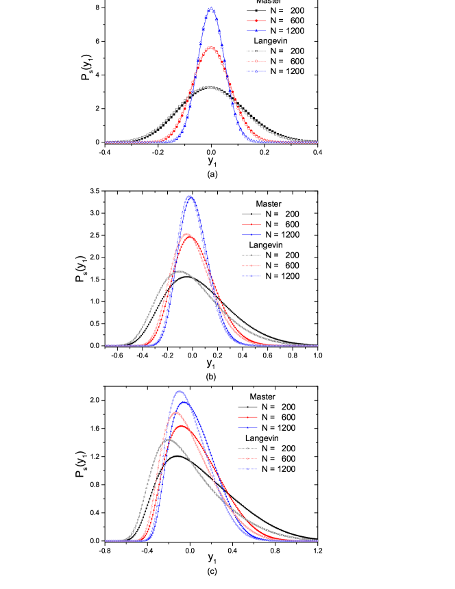
Figure 1: The steady-state probability density distributions $P_{s}\left(y_{1}\right)$, obtained from the master and the Langevin equations, as functions of $y_{1}$: $\left(a\right)$ $b=1.0$ and $\lambda_{R}=-0.5$, $\left(b\right)$ $b=1.8$ and $\lambda_{R}=-0.1$, and $\left(c\right)$ $b=1.98$ and $\lambda_{R}=-0.01$ with $N=200$, $600$, and $1200$.

The variance of steady-state probability density distribution is calculated and analyzed to reveal more informations about the distributions in different formulations, in particular, about the reliability of linearized Langevin equation. We show the logarithm of variance, $\ln\sigma_{s}^{2}\left(y_{1}\right)$, as a function of the logarithm of $\lambda_{R}$, $\ln\lambda_{R}$, for systems with $N=200$, $600$, and $1200$ in Fig. 2. Our results indicate that the variances obtained from master equation are, in general, larger than those obtained from Langevin equation. Note that the variances obtained from linearized Langevin are even larger than those from master, and there are big deviations from the results of master and Langevin for $0>\lambda_{R}>-0.25$ with $N=200$, $0>\lambda_{R}>-0.15$ with $N=600$, and $0>\lambda_{R}>-0.1$ with $N=1200$, and the results tend to diverge for $\lambda_{R}\rightarrow 0_{-}$ as shown in Fig. 2. Thus, the linearization scheme of Langevin equation becomes highly unreliable for systems with very small $\left|\lambda_{R}\right|$ and $\lambda_{R}<0$.

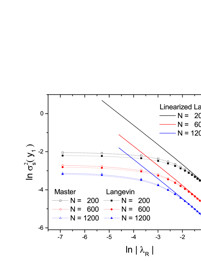
Figure 2: The logarithm of variance of steady-state probability density distribution, $\ln\sigma_{s}^{2}\left(y_{1}\right)$, obtained from the master, the Langevin, and the linearized Langevin equations, as a function of the logarithm of the absolute value of $\lambda_{R}$, $\ln\left|\lambda_{R}\right|$, for systems with $N=200$, $600$, and $1200$. The results of linearized Langevin equation are obtained from Eq. (36).

The power spectrum provides another aspect for the kinematic properties of systems. Since power spectrum defined in frequency space is complementary to probability density distribution defined in state space, a steady-state probability density distribution with smaller variance would correspond to the power spectrum covering a wider range of frequency. The results of power spectra for systems with $N=200$ and $1200$ are shown as ln$\left(NS_{1}\left(\omega\right)\right)$ vs. $\omega$ for $\lambda_{R}=-0.5$, $-0.1$, and $-0.01$ in Fig. 3. As shown in Figs. 3(c) and 3(d), the spectra obtained from linearized Langevin equation deviate significantly from those obtained from master and Langevin equations. Moreover, the peaks of the spectra from three different formulations locate at $\omega=\lambda_{I}$ for systems closed to the bifurcation line $\lambda_{R}=0$, this is consistent with the analytic result of linearized Langevin equation given by Eq. (47) which clearly indicates that the spectrum develops a pole of second order as $1/\left(\omega-\lambda_{I}\right)^{2}$ at the bifurcation line $\lambda_{R}=0$, although the pole is absent for master and Langevin equations.

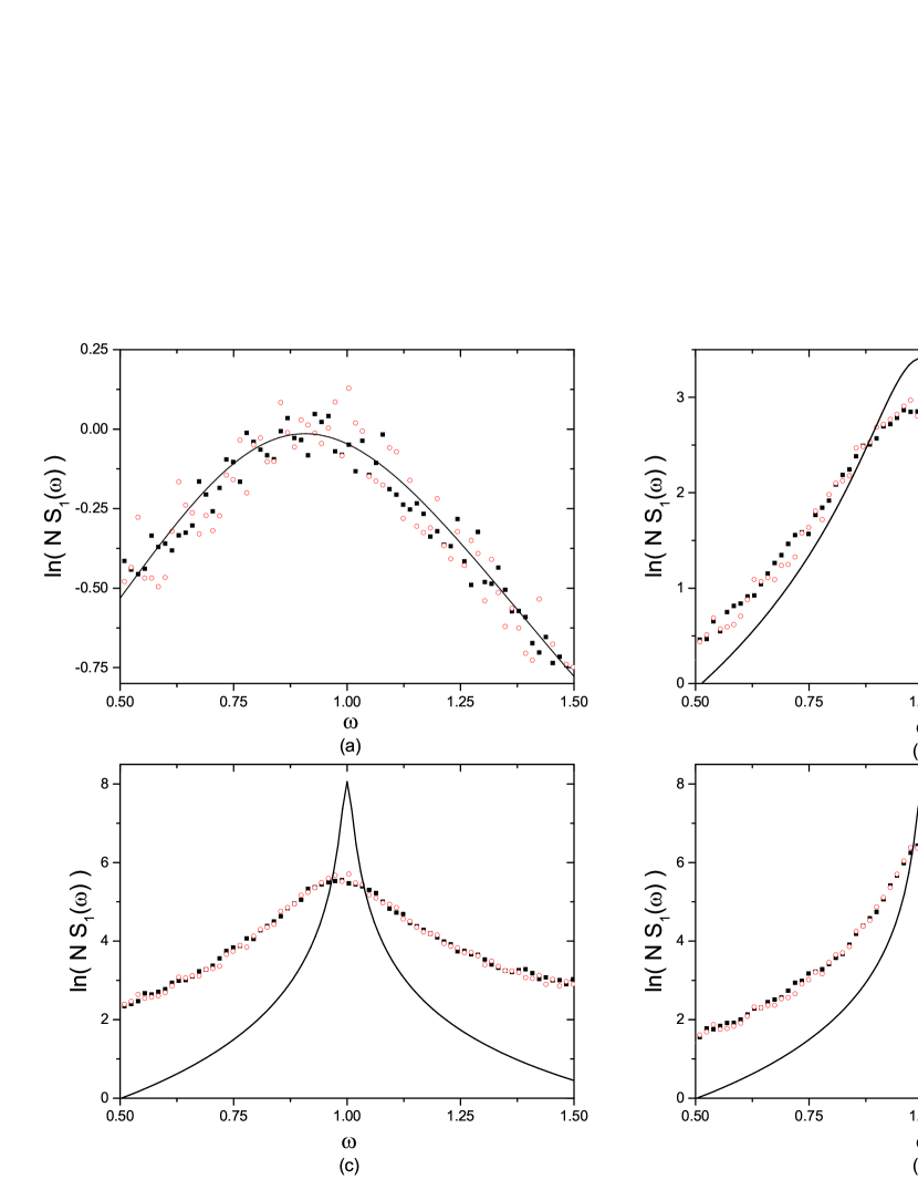
Figure 3: The logarithm of power spectrum, $\ln\left(NS_{1}\left(\omega\right)\right)$, obtained from the master (squares), the Langevin (circles), and linearized Langevin (solid lines) equations, as a function of $\omega$: $\left(a\right)$ $\lambda_{R}=-0.5$ and $N=200$, $\left(b\right)$ $\lambda_{R}=-0.1$ and $N=200$, $\left(c\right)$ $\lambda_{R}=-0.01$ and $N=200$, and $\left(d\right)$ $\lambda_{R}=-0.01$ and $N=1200$. The results of linearized Langevin equation are obtained from Eq. (47).

V Summary  

Three different formulations, including master, Langevin, and linearized Langevin equations, are used to analyze the effect of intrinsic fluctuations for chemical reactions defined by the Brusselator model. The systems are assumed to be in the phase of spirally stable fixed point for the deterministic mean-field equation, and we analyze the effect of intrinsic fluctuations based on steady-state probability density distributions in state space and power spectra in frequency space. Moreover, the differences between the results obtained from three formulations are investigated by considering two factors, the system size and the distance from the Hopf bifurcation line $\lambda_{R}=0$ for a spirally stable equilibrium state.

Our results indicate that the effect of intrinsic fluctuations based on master equation gives larger variance in steady-state probability density distribution than that obtained from Langevin equation, and the difference in the variance of distribution is enhanced when the system size is reduced. Moreover, the difference between the results of two formulations increases significantly when the equilibrium state is closed to the bifurcation line $\lambda_{R}=0$. In general, the discrepancy between the results of master and Langevin equations caused by the different distances of equilibrium states from the bifurcation line is more noticeable than that caused by the different system sizes.

Our results also show that the effect of intrinsic fluctuations revealed from linearized Langevin equation agrees very well with those obtained from Langevin equation for system far away from the bifurcation line. However, the linearization scheme of Langevin equation becomes inadequate for system closed to the bifurcation line. As $\lambda_{R}\rightarrow 0_{-}$, our analytic results indicate that the variance associated with the steady-state probability density function possesses a divergence as $1/\left|\lambda_{R}\right|$ and the power spectrum tends to diverge at $\omega=$ $\lambda_{I}$ as $1/\left(\omega-\lambda_{I}\right)^{2}$; these singular behaviors are absent in the results obtained from master and Langevin equations.

In conclusion, our results provide insights on the adequacy of different approaches for taking account of the intrinsic fluctuations into a system. Although the study is based on the Brusselator model, our results about the discrepancy between three frameworks can be quite general.

References

- (1) J.D. Crawford, Rev. Mod. Phys., 63, 991, (1991).
- (2) V.I. Arnold, Geometrical Methods in the Theory of Ordinary Differential Equations, Springer-Verlag New York(1983).
- (3) S.H. Strogatz, Nonlinear Dynamics and Chaos, 2nd edn, Westview Press (2014).
- (4) K. Tomita, T. Ohta, and H. Tomita, Prog. Theor. Phys., 52, 1744, (1974).
- (5) R.P. Boland, T. Galla, and A.J. McKane, J. Stat. Mech.: Theory and Experiment, 9, P09001, (2008).
- (6) A.J. McKane and T.J. Newman, Phys. Rev. Lett., 94, 218102, (2005).
- (7) A.A. Moreira, A. Mathur, D. Diermeier, and L.A.N. Amaral, Proc. Natl. Acad. Sci., 101, 12085, (2004).
- (8) M.S. de la Lama, I.G. Szendro, J.R. Iglesias, and H.S. Wio, Eur. Phys. J., B51, 435, (2006).
- (9) M. Scott, B. Ingalls, and M. Kaern, Chaos, 16, 026107, (2006).
- (10) F. Moss and P.V.E. McClintock, Noise in Nonlinear Dynamics, Cambridge University Press, Cambridge(1989)
- (11) N.G. van Kampen, Stochastic Processes in Physics and Chemistry, 3rd edn, Elsevier, Amsterdam(2007).
- (12) F. Sagues, J.M. Sancho, and J. Garcia-Ojalvo, Rev. Mod. Phys. 79, 829, (2007).
- (13) C.W. Gardiner, Handbook of Stochastic Method for Physics, Chemistry and the Natural Sciences, Spring-Verlag New York(1994).
- (14) H. Risken, The Fokker-Planck Equation: Methods of Solution and Applications, Springer, Berlin (1989)
- (15) P. Gaspard, J. Chem. Phys. 117, 8905, (2002).
- (16) H. Nakanishi, T. Sakaue, and J. Wakou, J. Chem. Phys. 139, 214105, (2013).
- (17) C. Van den Broeck, M. Malek, and F. Baras, J. Stat. Phys. 28, 557, (1982).
- (18) W. Vance and J. Ross, J. Chem. Phys. 105 (2), 479, (1996).
- (19) F. Mori and A.S. Mikhailov, Phys. Rev. E93, 062206, (2016).
- (20) C. Xue and N. Goldenfeld, Phy. Rev. Lett., 119, 268101, (2017).
- (21) D.T. Gillespie, J. Chem. Phys. 113, 297, (2000).
- (22) D.T. Gillespie, J. Phys. Chem. A 106, 5063, (2002).
- (23) D.T. Gillespie, Am. J. Phys. 64, 1246, (1996).
- (24) D.T. Gillespie, Annu. Rev. Phys. Chem. 58, 35, (2007).