Structure-preserving strategy for conservative simulation of relativistic nonlinear Landau–Fokker–Planck equation

Abstract

Mathematical symmetries of the Beliaev–Budker kernel are the most important structure of the relativistic Landau–Fokker–Planck equation. By preserving the beautiful symmetries, a mass-momentum-energy-conserving simulation has been demonstrated without any artificial constraints.

I Introduction

The Landau–Fokker–Planck (LFP) equation in the International System of Units is Lifshitz and Pitaevskii (1981)

$$\frac{\partial f_{\mathrm{s}}}{\partial t}=\frac{\Gamma}{2m_{\mathrm{s}}^{2}}\frac{\partial}{\partial\mathbf{u}}\cdot\int\mathsf{U}(\mathbf{u},\mathbf{u^{\prime}})\cdot\left(f_{\mathrm{s^{\prime}}}\frac{\partial f_{\mathrm{s}}}{\partial\mathbf{u}}-\frac{m_{\mathrm{s}}}{m_{\mathrm{s^{\prime}}}}f_{\mathrm{s}}\frac{\partial f_{\mathrm{s^{\prime}}}}{\partial\mathbf{u^{\prime}}}\right)\mathrm{d}\mathbf{u^{\prime}},$$ (1)

where $\Gamma=(q_{\mathrm{s}}^{2}q_{\mathrm{s^{\prime}}}^{2}\log\Lambda)/4\pi{\varepsilon_{0}}^{2}$, $\log\Lambda$ is the Coulomb logarithm, $\varepsilon_{0}$ is the vacuum permittivity, $(f_{\mathrm{s}},f_{\mathrm{s^{\prime}}})$, $(m_{\mathrm{s}},m_{\mathrm{s^{\prime}}})$, $(q_{\mathrm{s}},q_{\mathrm{s^{\prime}}})$ and $(\mathbf{u},\mathbf{u^{\prime}})$ are the distribution function, mass, electric charge and momentum per unit mass of species $(\mathrm{s},\mathrm{s^{\prime}})$, respectively. In the relativistic case, the collision kernel $\mathsf{U}(\mathbf{u},\mathbf{u^{\prime}})$ is described as follows Beliaev and Budker (1956):

$$\mathsf{U}=\frac{r^{2}}{\gamma\gamma^{\prime}w^{3}}\left[w^{2}\mathsf{I}-\gamma^{2}\mathbf{vv}-\gamma^{\prime 2}\mathbf{v^{\prime}v^{\prime}}+r\gamma\gamma^{\prime}(\mathbf{vv^{\prime}}+\mathbf{v^{\prime}v})\right],$$ (2)

where $r=\gamma\gamma^{\prime}(1-\mathbf{v}\cdot\mathbf{v^{\prime}}/c^{2})$, $w=c\sqrt{r^{2}-1}$, $\mathbf{v}=\mathbf{u}/\gamma$, $\mathbf{v^{\prime}}=\mathbf{u^{\prime}}/\gamma^{\prime}$, and $c$ is the speed of light in vacuum. The Lorentz factor is defined as follows:

$$\gamma=\sqrt{1+|\mathbf{u}/c|^{2}}=1/\sqrt{1-|\mathbf{v}/c|^{2}},$$ (3)

$$\gamma^{\prime}=\sqrt{1+|\mathbf{u^{\prime}}/c|^{2}}=1/\sqrt{1-|\mathbf{v^{\prime}}/c|^{2}}.$$ (4)

The relativistic LFP equation is designed so as to ensure the mass-momentum-energy conservation and the H-theorem.

The collisional processes described by the relativistic LFP equation are essential in fusion plasmas. In practical simulations, the relativistic LFP equation is often linearized so that the computational cost is reduced from $O(N^{2})$ to $O(N)$, where $N$ is the number of unknowns. For fast ignition, which heats the imploded core by relativistic fast electrons, of inertial confinement fusion Tabak et al. (1994), a linearization of Nakashima and Takabe Nakashima and Takabe (2002) is employed by relativistic Fokker–Planck codes such as RFP-2D Yokota et al. (2006), FIBMET Johzaki et al. (2009) and FIDO Sherlock (2009); Ridgers et al. (2011). The linearization is based on the fact that the colliding particles are much faster than the collided ones. This violates symmetry of the collision kernel so the conservation laws are maintained only at the continuous limit. For runaway electrons in tokamak disruptions Dreicer (1959), linearization which assumes an weakly relativistic equilibrium background Karney and Fisch (1985); Karney (1986) is sometimes performed to take into account the effect of non-thermal electrons Nuga et al. (2016), while the conservation laws are violated. Further, TASK/FP Nuga and Fukuyama (2011) and CQL3D Petrov and Harvey (2016) codes have options that decompose the nonlinear LFP equation into Legendre modes and solve first a few modes. The Legendre polynomials ensure the mass-momentum-energy conservation limit to resolve structures of the pitch angle. Recently, Stahl et al. developed NORSE code Stahl et al. (2017) which models nonlinear electron–electron collisions by the Braams–Karney potential formulation Braams and Karnel (1987). However, the NORSE code violates the conservation laws including the mass conservation. In the potential form, the “nonlinear constraints” is one of the ways to preserve the conservation laws Taitano et al. (2015) and equilibrium state Taitano et al. (2017), i.e. one of the projection method in the literature of applied mathematics Eich (1993). However, the projection method can affect the stability of numerical schemes, and it may not be suit for long time-scale simulations. In magnetohydrodynamics simulations, for example, the projection method Brackbill and Barnes (1980) or constrained transport (CT) method Evans and Hawley (1988) has been used to enforce the solenoidal constraint ($\nabla\cdot\mathbf{B}=0$). However, such an inconsistent magnetic field can induce “checkerboard phenomenon” which is one of the numerical instabilities Flock et al. (2010).

Unlike the relativistic regime, many non-relativistic structure-preserving schemes have been proposed to ensure the conservation laws, positivity and H-theorem. Chang and Cooper developed a positivity-preserving scheme for one-dimensional (1D) linearized LFP equation Chang and Cooper (1970), and it was extended to nonlinear isotropic LFP equation Buet and Cordier (2002) and nonlinear multi-dimensional one Yoon and Chang (2014a, b); Hager et al. (2016) preserving the conservation laws and H-theorem. A structure-preserving finite-element scheme Hirvijoki and Adams (2017) is also developed to ensure the conservation laws on unstructure meshes. These works are based on a weak-form associated with Eq. (1). The integrand of Eq. (1) can be transformed into the following one analytically:

$$f_{\mathrm{s}}f_{\mathrm{s^{\prime}}}\mathsf{U}(\mathbf{u},\mathbf{u^{\prime}})\cdot\left(\frac{\partial\log f_{\mathrm{s}}}{\partial\mathbf{u}}-\frac{m_{\mathrm{s}}}{m_{\mathrm{s^{\prime}}}}\frac{\partial\log f_{\mathrm{s^{\prime}}}}{\partial\mathbf{u^{\prime}}}\right).$$ (5)

The weak-form coming from Eq. (5) is called as “log” weak-form, and the proof of H-theorem by the log weak-form is straightforward. An analytical discussion was first given by Pekker and Khudik Pekker and Khudik (1984), and conservative and entropic discretizations have been proposed for isotropic Berezin et al. (1987); Buet and Cordier (1998) and multi-dimensional cases Degond and Lucquin-Desreux (1994); Buet et al. (1997). Furthermore, an energy-conserving LFP scheme with the Rosenbluth potential form Rosenbluth et al. (1957) was proposed using an analogy of the Maxwell stress tensor in electromagnetism Chacón et al. (2000a, b). However, structure-preserving schemes for the relativistic LFP equation have not been developed since the Lorentz factor is not expressed as polynomials of finite-order in the momentum Hirvijoki and Adams (2017).

In this paper, we demonstrate a structure-preserving simulation of the relativistic LFP equation which strictly preserve the conservation laws of mass, momentum and energy. The key concept is the same with our recent work about a quadratic conservative scheme for the relativistic Vlasov–Maxwell system Shiroto et al. (2019). Moreover, a similar approach has been used in a non-relativistic scheme with non-uniform meshes Buet and Thanh (2006, 2007). The rest of this paper is composed as follows. Section II shows an intuitive discretization which cannot maintain the energy conservation. Section III deductively derives requirements for the conservation laws in discrete form. Our structure-preserving scheme and its concept are introduced in Sec. IV. A verification of conservation property through a thermal-equilibration is performed in Sec. V. Section VI is conclusions of this article.

II CONVENTIONAL SCHEME

In this article, the relativistic LFP equation is discretized as follows. Note that the conservation laws are not affected by the temporal structure, so only momentum dimensions are discretized here:

$$\frac{\partial{f_{\mathrm{s}}}^{\mathbf{j}}}{\partial t}\equiv\frac{\Gamma}{2{m_{\mathrm{s}}}^{2}}\frac{\delta}{\delta\mathbf{u}}\cdot\sum_{\mathbf{k}} \mathsf{U}(\mathbf{u^{j}},\mathbf{{u^{\prime}}^{k}})\cdot$$

$$\left({f_{\mathrm{s^{\prime}}}}^{\mathbf{k}}\frac{\delta{f_{\mathrm{s}}}^{\mathbf{j}}}{\delta\mathbf{u}}-\frac{m_{\mathrm{s}}}{m_{\mathrm{s^{\prime}}}}{f_{\mathrm{s}}}^{\mathbf{j}}\frac{\delta{f_{\mathrm{s^{\prime}}}}^{\mathbf{k}}}{\delta\mathbf{u^{\prime}}}\right)\Delta\mathbf{u^{\prime}},$$ (6)

where $\mathbf{j}\equiv[j_{1},j_{2},j_{3}]$ and $\mathbf{k}\equiv[k_{1},k_{2},k_{3}]$ are the indices of uniform momentum grids for $\mathbf{u}$ and $\mathbf{u^{\prime}}$, respectively. $\Delta\mathbf{u}\equiv\Delta u_{1}\Delta u_{2}\Delta u_{3}$, and $(\Delta u_{1},\Delta u_{2},\Delta u_{3})$ is the grid interval of $(u_{1},u_{2},u_{3})$. The species $(\mathrm{s},\mathrm{s^{\prime}})$ use the same momentum grids $(\mathbf{u^{j}}=\mathbf{{u^{\prime}}^{j}},\Delta\mathbf{u}=\Delta\mathbf{u^{\prime}})$. Here we use a second-order central difference for simplicity:

$$\frac{\delta a^{\mathbf{j},\mathbf{k}}}{\delta u_{1}}\equiv\frac{a^{j_{1}+1,j_{2},j_{3},k_{1},k_{2},k_{3}}-a^{j_{1}-1,j_{2},j_{3},k_{1},k_{2},k_{3}}}{2\Delta u_{1}},$$

$$\frac{\delta a^{\mathbf{j},\mathbf{k}}}{\delta u_{2}}\equiv\frac{a^{j_{1},j_{2}+1,j_{3},k_{1},k_{2},k_{3}}-a^{j_{1},j_{2}-1,j_{3},k_{1},k_{2},k_{3}}}{2\Delta u_{2}},$$

$$\frac{\delta a^{\mathbf{j},\mathbf{k}}}{\delta u_{3}}\equiv\frac{a^{j_{1},j_{2},j_{3}+1,k_{1},k_{2},k_{3}}-a^{j_{1},j_{2},j_{3}-1,k_{1},k_{2},k_{3}}}{2\Delta u_{3}},$$

$$\frac{\delta a^{\mathbf{j},\mathbf{k}}}{\delta u^{\prime}_{1}}\equiv\frac{a^{j_{1},j_{2},j_{3},k_{1}+1,k_{2},k_{3}}-a^{j_{1},j_{2},j_{3},k_{1}-1,k_{2},k_{3}}}{2\Delta u^{\prime}_{1}},$$

$$\frac{\delta a^{\mathbf{j},\mathbf{k}}}{\delta u^{\prime}_{2}}\equiv\frac{a^{j_{1},j_{2},j_{3},k_{1},k_{2}+1,k_{3}}-a^{j_{1},j_{2},j_{3},k_{1},k_{2}-1,k_{3}}}{2\Delta u^{\prime}_{2}},$$

$$\frac{\delta a^{\mathbf{j},\mathbf{k}}}{\delta u^{\prime}_{3}}\equiv\frac{a^{j_{1},j_{2},j_{3},k_{1},k_{2},k_{3}+1}-a^{j_{1},j_{2},j_{3},k_{1},k_{2},k_{3}-1}}{2\Delta u^{\prime}_{3}}.$$

where $a^{\mathbf{j},\mathbf{k}}\equiv a(\mathbf{u^{j}},\mathbf{u^{\prime k}})$ is an arbitrary function.

In an intuitive discretization, the collision kernel is calculated by its arguments directly:

$$\mathsf{U}(\mathbf{u^{j}},\mathbf{u^{\prime}}^{\mathbf{k}})\equiv\frac{(r^{\mathbf{j,k}})^{2}}{\gamma^{\mathbf{j}}{\gamma^{\prime}}^{\mathbf{k}}(w^{\mathbf{j,k}})^{3}}\left[(w^{\mathbf{j,k}})^{2}\mathsf{I}-\mathbf{u^{j}u^{j}}-\mathbf{{u^{\prime}}^{k}{u^{\prime}}^{k}}\right.$$

$$\left.+r^{\mathbf{j,k}}(\mathbf{u^{j}{u^{\prime}}^{k}}+\mathbf{{u^{\prime}}^{k}u^{j}})\right],$$ (7)

From the definition, the collision kernel Eq. (7) satisfies two mathematical symmetries:

$$\mathsf{U}(\mathbf{u^{j},{u^{\prime}}^{k}})=\mathsf{U}(\mathbf{{u^{\prime}}^{k},u^{j}}),$$ (8)

$$\mathsf{U}(\mathbf{u^{j}},\mathbf{{u^{\prime}}^{k}})\cdot\mathbf{v^{j}}=\mathsf{U}(\mathbf{{u^{\prime}}^{k}},\mathbf{u^{j}})\cdot\mathbf{{v^{\prime}}^{k}}.$$ (9)

III REQUIREMENTS FOR CONSERVATION LAWS IN DISCRETE FORM

In this section, requirements for the conservation laws are derived deductively. The mass conservation is trivially maintained, so the discussion is focused on the momentum-energy conservation. The following points are required to prove the conservation laws analytically from the relativistic LFP equation:

1. Integration-by-parts must be maintained.

2. $\mathsf{U}(\mathbf{u},\mathbf{u^{\prime}})=\mathsf{U}(\mathbf{u^{\prime}},\mathbf{u})$ is required for the momentum conservation.

3. $\mathsf{U}(\mathbf{u},\mathbf{u^{\prime}})\cdot\mathbf{v}=\mathsf{U}(\mathbf{u^{\prime}},\mathbf{u})\cdot\mathbf{v^{\prime}}$ is required for the energy conservation.

If one can assume $a^{\mathbf{j,k}}=0$ at the momentum boundaries, the following summation-by-parts, i.e. the integration-by-parts in discrete form, is valid:

$$\sum_{\mathbf{j,k}}\left(\frac{\delta a^{\mathbf{j,k}}}{\delta\mathbf{u}}b^{\mathbf{j,k}}\right)\Delta\mathbf{u}\Delta\mathbf{u^{\prime}}=-\sum_{\mathbf{j,k}}\left(a^{\mathbf{j,k}}\frac{\delta b^{\mathbf{j,k}}}{\delta\mathbf{u}}\right)\Delta\mathbf{u}\Delta\mathbf{u^{\prime}},$$

$$\sum_{\mathbf{j,k}}\left(\frac{\delta a^{\mathbf{j,k}}}{\delta\mathbf{u^{\prime}}}b^{\mathbf{j,k}}\right)\Delta\mathbf{u}\Delta\mathbf{u^{\prime}}=-\sum_{\mathbf{j,k}}\left(a^{\mathbf{j,k}}\frac{\delta b^{\mathbf{j,k}}}{\delta\mathbf{u^{\prime}}}\right)\Delta\mathbf{u}\Delta\mathbf{u^{\prime}},$$

where $b^{\mathbf{j,k}}$ is also an arbitrary function. Therefore, the first point is automatically preserved if a finite-difference operator has a linearity. In addition, the second point is naturally satisfied unless the Braams and Karney potential is employed. The most important discussion in our article is the third point. To satisfy $a^{\mathbf{j,k}}=0$ in the relativistic LFP equation, the computational domain must be large enough to ensure that the distribution function is negligible small at the boundary. In other words, no boundary condition can enforce all of the conservation laws.

III.A MOMENTUM CONSERVATION

The momentum of species “$\mathrm{s}$” is described as a first-order moment of Eq. (6):

$$\frac{\partial}{\partial t}\left(\sum_{\mathbf{j}}m_{\mathrm{s}}\mathbf{u^{j}}{f_{\mathrm{s}}}^{\mathbf{j}}\Delta\mathbf{u}\right)$$

$$= \frac{\Gamma}{2{m_{\mathrm{s}}}}\sum_{\mathbf{j}}\left[\mathbf{u^{j}}\frac{\delta}{\delta\mathbf{u}}\right.\cdot\sum_{\mathbf{k}}\mathsf{U}(\mathbf{u^{j}},\mathbf{{u^{\prime}}^{k}})\cdot$$

$$\qquad\qquad\left.\left({f_{\mathrm{s^{\prime}}}}^{\mathbf{k}}\frac{\delta{f_{\mathrm{s}}}^{\mathbf{j}}}{\delta\mathbf{u}}-\frac{m_{\mathrm{s}}}{m_{\mathrm{s^{\prime}}}}{f_{\mathrm{s}}}^{\mathbf{j}}\frac{\delta{f_{\mathrm{s^{\prime}}}}^{\mathbf{k}}}{\delta\mathbf{u^{\prime}}}\right)\Delta\mathbf{u^{\prime}}\right]\Delta\mathbf{u}$$

$$= -\frac{\Gamma}{2}\sum_{\mathbf{j,k}}\left[\mathsf{U}(\mathbf{u^{j}},\mathbf{{u^{\prime}}^{k}})\cdot\left(\frac{{f_{\mathrm{s^{\prime}}}}^{\mathbf{k}}}{m_{\mathrm{s}}}\frac{\delta{f_{\mathrm{s}}}^{\mathbf{j}}}{\delta\mathbf{u}}-\frac{{f_{\mathrm{s}}}^{\mathbf{j}}}{m_{\mathrm{s^{\prime}}}}\frac{\delta{f_{\mathrm{s^{\prime}}}}^{\mathbf{k}}}{\delta\mathbf{u^{\prime}}}\right)\right]\Delta\mathbf{u}\Delta\mathbf{u^{\prime}},$$

$$\left(\because\delta\mathbf{u^{j}}/\delta\mathbf{u}\mbox{ is an identity matrix.}\right)$$ (10)

Likewise, the momentum of species “$\mathrm{s^{\prime}}$” is obtained as follows:

$$\frac{\partial}{\partial t}\left(\sum_{\mathbf{k}}m_{\mathrm{s^{\prime}}}\mathbf{{u^{\prime}}^{k}}{f_{\mathrm{s^{\prime}}}}^{\mathbf{k}}\Delta\mathbf{u^{\prime}}\right)$$

$$= -\frac{\Gamma}{2}\sum_{\mathbf{j,k}}\left[\mathsf{U}(\mathbf{{u^{\prime}}^{k}},\mathbf{u^{j}})\cdot\left(\frac{{f_{\mathrm{s}}}^{\mathbf{j}}}{m_{\mathrm{s^{\prime}}}}\frac{\delta{f_{\mathrm{s^{\prime}}}}^{\mathbf{k}}}{\delta\mathbf{u^{\prime}}}-\frac{{f_{\mathrm{s^{\prime}}}}^{\mathbf{k}}}{m_{\mathrm{s}}}\frac{\delta{f_{\mathrm{s}}}^{\mathbf{j}}}{\delta\mathbf{u}}\right)\right]\Delta\mathbf{u}\Delta\mathbf{u^{\prime}}.$$ (11)

The temporal development of total momentum is obtained as a sum of Eqs. (10) and (11):

$$\frac{\partial}{\partial t}\left(\sum_{\mathbf{j}}m_{\mathrm{s}}\mathbf{{u}^{j}}{f_{\mathrm{s}}}^{\mathbf{j}}\Delta\mathbf{u}+\sum_{\mathbf{k}}m_{\mathrm{s^{\prime}}}\mathbf{{u^{\prime}}^{k}}{f_{\mathrm{s^{\prime}}}}^{\mathbf{k}}\Delta\mathbf{u^{\prime}}\right)$$

$$= -\frac{\Gamma}{2}\sum_{\mathbf{j,k}}\left[\left(\mathsf{U}(\mathbf{u^{j}},\mathbf{{u^{\prime}}^{k}})-\mathsf{U}(\mathbf{{u^{\prime}}^{k}},\mathbf{{u}^{j}})\right)\cdot\right.$$

$$\qquad\qquad\qquad\qquad\left.\left(\frac{{f_{\mathrm{s^{\prime}}}}^{\mathbf{k}}}{m_{\mathrm{s}}}\frac{\delta{f_{\mathrm{s}}}^{\mathbf{j}}}{\delta\mathbf{u}}-\frac{{f_{\mathrm{s}}}^{\mathbf{j}}}{m_{\mathrm{s^{\prime}}}}\frac{\delta{f_{\mathrm{s^{\prime}}}}^{\mathbf{k}}}{\delta\mathbf{u^{\prime}}}\right)\right]\Delta\mathbf{u}\Delta\mathbf{u^{\prime}}.$$ (12)

Therefore, the intuitive kernel of Eq. (7) strictly maintains the momentum conservation owing to Eq. (8).

III.B ENERGY CONSERVATION

The energy of species “$\mathrm{s}$” is described as a second-order moment of Eq. (6):

$$\frac{\partial}{\partial t}\left(\sum_{\mathbf{j}}m_{\mathrm{s}}c^{2}\gamma^{\mathbf{j}}{f_{\mathrm{s}}}^{\mathbf{j}}\Delta\mathbf{u}\right)$$

$$= \frac{\Gamma}{2{m_{\mathrm{s}}}}\sum_{\mathbf{j}}\left[\gamma^{\mathbf{j}}c^{2}\frac{\delta}{\delta\mathbf{u}}\right.\cdot\sum_{\mathbf{k}}\mathsf{U}(\mathbf{u^{j}},\mathbf{{u^{\prime}}^{k}})\cdot$$

$$\qquad\qquad\left.\left({f_{\mathrm{s^{\prime}}}}^{\mathbf{k}}\frac{\delta{f_{\mathrm{s}}}^{\mathbf{j}}}{\delta\mathbf{u}}-\frac{m_{\mathrm{s}}}{m_{\mathrm{s^{\prime}}}}{f_{\mathrm{s}}}^{\mathbf{j}}\frac{\delta{f_{\mathrm{s^{\prime}}}}^{\mathbf{k}}}{\delta\mathbf{u^{\prime}}}\right)\Delta\mathbf{u^{\prime}}\right]\Delta\mathbf{u}$$

$$= -\frac{\Gamma}{2}\sum_{\mathbf{j,k}}\left[\mathsf{U}(\mathbf{u^{j}},\mathbf{{u^{\prime}}^{k}})\cdot\frac{\delta(\gamma^{\mathbf{j}}c^{2})}{\delta\mathbf{u}}\cdot\right.$$

$$\qquad\qquad\qquad\left.\left(\frac{{f_{\mathrm{s^{\prime}}}}^{\mathbf{k}}}{m_{\mathrm{s}}}\frac{\delta{f_{\mathrm{s}}}^{\mathbf{j}}}{\delta\mathbf{u}}-\frac{{f_{\mathrm{s}}}^{\mathbf{j}}}{m_{\mathrm{s^{\prime}}}}\frac{\delta{f_{\mathrm{s^{\prime}}}}^{\mathbf{k}}}{\delta\mathbf{u^{\prime}}}\right)\right]\Delta\mathbf{u}\Delta\mathbf{u^{\prime}}.$$ (13)

Likewise, the energy of species “$\mathrm{s^{\prime}}$” is obtained as follows:

$$\frac{\partial}{\partial t}\left(\sum_{\mathbf{k}}m_{\mathrm{s^{\prime}}}c^{2}{\gamma^{\prime}}^{\mathbf{k}}{f_{\mathrm{s^{\prime}}}}^{\mathbf{k}}\Delta\mathbf{u^{\prime}}\right)$$

$$= -\frac{\Gamma}{2}\sum_{\mathbf{j,k}}\left[\mathsf{U}(\mathbf{{u^{\prime}}^{k}},\mathbf{{u}^{j}})\cdot\frac{\delta({\gamma^{\prime}}^{\mathbf{k}}c^{2})}{\delta\mathbf{u^{\prime}}}\cdot\right.$$

$$\qquad\qquad\qquad\left.\left(\frac{{f_{\mathrm{s}}}^{\mathbf{j}}}{m_{\mathrm{s^{\prime}}}}\frac{\delta{f_{\mathrm{s^{\prime}}}}^{\mathbf{k}}}{\delta\mathbf{u^{\prime}}}-\frac{{f_{\mathrm{s^{\prime}}}}^{\mathbf{k}}}{m_{\mathrm{s}}}\frac{\delta{f_{\mathrm{s}}}^{\mathbf{j}}}{\delta\mathbf{u}}\right)\right]\Delta\mathbf{u^{\prime}}\Delta\mathbf{u}.$$ (14)

The temporal development of total energy is obtained as a sum of Eqs. (13) and (14):

$$\frac{\partial}{\partial t}\left(\sum_{\mathbf{j}}m_{\mathrm{s}}c^{2}\gamma^{\mathbf{j}}{f_{\mathrm{s}}}^{\mathbf{j}}\Delta\mathbf{u}+\sum_{\mathbf{k}}m_{\mathrm{s^{\prime}}}c^{2}{\gamma^{\prime}}^{\mathbf{k}}{f_{\mathrm{s^{\prime}}}}^{\mathbf{k}}\Delta\mathbf{u^{\prime}}\right)$$

$$= -\frac{\Gamma}{2}\sum_{\mathbf{j,k}}\left[\left(\mathsf{U}(\mathbf{u^{j}},\mathbf{{u^{\prime}}^{k}})\cdot\mathbf{\bar{v}}-\mathsf{U}(\mathbf{{u^{\prime}}^{k}},\mathbf{{u}^{j}})\cdot\mathbf{\bar{v}^{\prime}}\right)\cdot\right.$$

$$\qquad\qquad\qquad\qquad\left.\left(\frac{{f_{\mathrm{s^{\prime}}}}^{\mathbf{k}}}{m_{\mathrm{s}}}\frac{\delta{f_{\mathrm{s}}}^{\mathbf{j}}}{\delta\mathbf{u}}-\frac{{f_{\mathrm{s}}}^{\mathbf{j}}}{m_{\mathrm{s^{\prime}}}}\frac{\delta{f_{\mathrm{s^{\prime}}}}^{\mathbf{k}}}{\delta\mathbf{u^{\prime}}}\right)\right]\Delta\mathbf{u}\Delta\mathbf{u^{\prime}},$$ (15)

where the velocities with overlines are defined as follows:

$$\mathbf{\bar{v}}\equiv\frac{\delta(\gamma^{\mathbf{j}}c^{2})}{\delta\mathbf{u}},\quad\mathbf{\bar{v}}^{\prime}\equiv\frac{\delta({\gamma^{\prime}}^{\mathbf{k}}c^{2})}{\delta\mathbf{u^{\prime}}}.$$ (16)

Therefore, $\mathsf{U}(\mathbf{u^{j}},\mathbf{{u^{\prime}}^{k}})\cdot\mathbf{\bar{v}}=\mathsf{U}(\mathbf{{u^{\prime}}^{k}},\mathbf{u^{j}})\cdot\mathbf{\bar{v}^{\prime}}$ is required for the energy conservation in discrete form. The intuitive kernel Eq. (7) satisfies Eq. (9), so the energy conservation would be preserved even in discrete form if $\mathbf{\bar{v}}=\mathbf{v^{j}}$ and $\mathbf{\bar{v}^{\prime}}=\mathbf{{v^{\prime}}^{k}}$ were true. Generally speaking, the proposition is false resulting in a violation of the energy conservation. For the second-order central difference;

$$(\gamma^{j_{1}+1,j_{2},j_{3}})^{2}-(\gamma^{j_{1}-1,j_{2},j_{3}})^{2}=({u_{1}}^{j_{1}+1}/c)^{2}-({u_{1}}^{j_{1}-1}/c)^{2},$$

$$\therefore\bar{v}_{1}=\frac{\delta(\gamma^{\mathbf{j}}c^{2})}{\delta u_{1}}=\frac{2{u_{1}}^{j_{1}}}{\gamma^{j_{1}+1,j_{2},j_{3}}+\gamma^{j_{1}-1,j_{2},j_{3}}}\neq\frac{{u_{1}}^{j_{1}}}{\gamma^{j_{1},j_{2},j_{3}}}.$$

The only exception is the non-relativistic limit when the Lorentz factor is always unity. Hirvijoki and Adams reported that their scheme cannot maintain the exact energy conservation in the relativistic regime Hirvijoki and Adams (2017), and our discussion should be connected on the fundamental level with this issue although their discussion was based on the finite-element method.

IV STRUCTURE-PRESERVING STRATEGY

Here we propose a structure-preserving scheme for the relativistic LFP equation which resolves the energy-conservation problem of the intuitive scheme. According to Eqs. (12) and (15), the following discrete requirements must be preserved to maintain the mass-momentum-energy conservation:

1. Summation-by-parts

2. $\mathsf{U}(\mathbf{u^{j}},\mathbf{{u^{\prime}}^{k}})=\mathsf{U}(\mathbf{{u^{\prime}}^{k}},\mathbf{u^{j}})$

3. $\mathsf{U}(\mathbf{u^{j}},\mathbf{{u^{\prime}}^{k}})\cdot\mathbf{\bar{v}}=\mathsf{U}(\mathbf{{u^{\prime}}^{k}},\mathbf{u^{j}})\cdot\mathbf{\bar{v}^{\prime}}$

The following is the only Beliaev–Budker kernel that preserves the above requirements:

$$\mathsf{U}(\mathbf{u^{j}},\mathbf{u^{\prime}}^{\mathbf{k}})\equiv\frac{\bar{r}^{2}}{\bar{\gamma}\bar{\gamma}^{\prime}\bar{w}^{3}}\left[\bar{w}^{2}\mathsf{I}-\bar{\gamma}^{2}\mathbf{\bar{v}\bar{v}}-\bar{\gamma}^{\prime 2}\mathbf{\bar{v}^{\prime}\bar{v}^{\prime}}\right.$$

$$\left.+\bar{r}\bar{\gamma}\bar{\gamma}^{\prime}(\mathbf{\bar{v}\bar{v}^{\prime}+\bar{v}^{\prime}\bar{v}})\right],$$ (17)

where the variables with overlines are

$$\bar{\gamma}\equiv 1/\sqrt{1-|\bar{\mathbf{v}}/c|^{2}}\neq\gamma^{\mathbf{j}},\quad\bar{\gamma}^{\prime}\equiv 1/\sqrt{1-|\bar{\mathbf{v}}^{\prime}/c|^{2}}\neq{\gamma^{\prime}}^{\mathbf{k}},$$

$$\bar{r}\equiv\bar{\gamma}\bar{\gamma}^{\prime}(1-\bar{\mathbf{v}}\cdot\bar{\mathbf{v}}^{\prime})\neq r^{\mathbf{j,k}},\quad\bar{w}\equiv c\sqrt{\bar{r}^{2}-1}\neq w^{\mathbf{j,k}}.$$

A combination of Eqs. (6) and (17) naturally preserves the law of energy conservation naturally. However, the positivity of distribution function and H-theorem are not guaranteed unconditionally by this formulation. We do not give a discussion of the temporal discretization in this article, which is done in the papers about entropic schemes.

V DEMONSTRATION

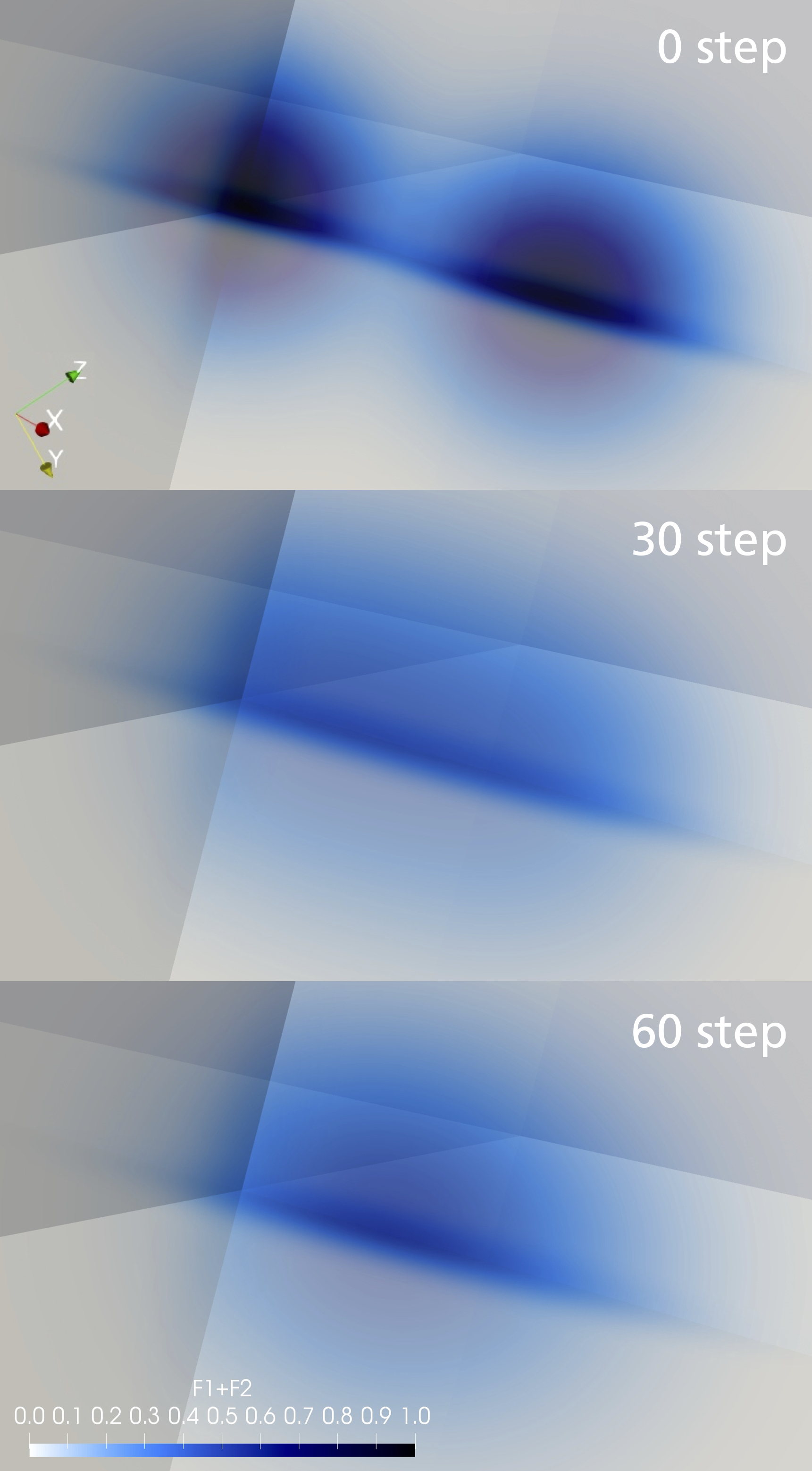
Figure 1: (Color online) Time development of distribution function initialized by double Maxwell–Jüttner distribution.

(a) Structure-preserving discretization (proposed).

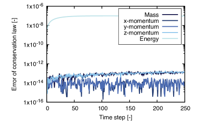
(b) Intuitive discretization (conventional).

Figure 2: Conservation errors for mass, momentum and energy in a thermal-equilibration verification.

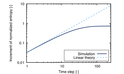
Figure 3: (Color online) Verification of H-theorem. Caution: the proposed scheme does not ensure the H-theorem mathematically.

To verify the proposed scheme, a collisional relaxation of a particle–antiparticle plasma is calculated for simplicity ($m_{\mathrm{s}}=m_{\mathrm{s^{\prime}}}\equiv m,q_{\mathrm{s}}=-q_{\mathrm{s^{\prime}}}\equiv q$). The particles and antiparticles are initialized by the following shifted Maxwell–Jüttner distrubtions Zenitani (2015).

$$f_{\mathrm{s}}(\mathbf{u})=\exp\left(-\frac{\gamma-1}{\theta}\right),$$

$$f_{\mathrm{s^{\prime}}}(\mathbf{u^{\prime}})=\frac{1}{\gamma_{0}}\exp\left(-\frac{\gamma^{\prime}\gamma_{0}-\gamma_{0}\mathbf{v}_{0}\cdot\mathbf{u^{\prime}}/c^{2}-1}{\theta}\right),$$

where $\theta=0.01$ is the temperature normalized by the rest mass energy, $\mathbf{v}_{0}/c=^{\mathrm{T}}[0.2,0.2,0.2]$, and $\gamma_{0}=1/\sqrt{1-\mathbf{v}_{0}\cdot\mathbf{v}_{0}/c^{2}}$. The computational domain is set to be $\{(u_{1},u_{2},u_{3})|-1.2c\leq u_{1},u_{2},u_{3}\leq 1.8c\}$, and the number of computational cells is $128\times 128\times 128$. In this verification, a first-order Euler explicit method is used as a time integration. The temporal interval is given as $\Gamma m^{-2}\Delta t=1/80$, so that the temporal resolution is fine enough to see the relaxation. In this test, only unlike-particle collisions are considered.

Figure 1 shows a time development of the double Maxwell–Jüttner distribution through the collisional relaxation. The double-peaked distribution function approximates to the equilibrium state whose velocity shift and temperature are $\mathbf{v}_{0}/2$ and $2\theta$, respectively. Figures 2(a) and (b) indicate the errors of conservation laws for the structure-preserving and intuitive discretizations, respectively. The structure-preserving scheme with the collision kernel of Eq. (17) strictly preserves the conservation laws of mass, momentum and energy only with round-off errors. It seems that the mass, momentum of $z$-direction and energy slightly accumulate the round-off errors. We reported that Padé-type (or implicit) filters used in computational fluid dynamics can accumulate round-off errors, but it can be suppressed by changing the order of arithmetic operations Shiroto et al. (2017). Therefore, the accumulation of round-off errors can be resolved by an optimization of the code although it is out of scope of this article. From the other perspective, the conservation property of the proposed scheme is quite fine as well as it is affected by the order of arithmetic operations. In contrast, the intuitive discretization with the collision kernel of Eq. (7) clearly violates the energy conservation. Note that the mass and momentum are strictly conserved with the intuitive scheme. This is because the relativistic LFP equation is discretized in the divergence-form, and the intuitive collision kernel also satisfies the symmetry of $\mathsf{U}(\mathbf{u},\mathbf{u^{\prime}})=\mathsf{U}(\mathbf{u^{\prime}},\mathbf{u})$.

Finally, we address some remaining issues about the positivity and H-theorem. Figure 3 shows the H-theorem is strictly preserved and the linear relaxation rate is initially reproduced well in the current situation. Here we introduced the entropy as follows to avoid negative values due to round-off errors:

$$S\equiv-\sum_{\mathbf{j}}|{f_{\mathrm{s}}}^{\mathbf{j}}|\log|{f_{\mathrm{s}}}^{\mathbf{j}}|\Delta\mathbf{u}-\sum_{\mathbf{k}}|{f_{\mathrm{s^{\prime}}}}^{\mathbf{k}}|\log|{f_{\mathrm{s^{\prime}}}}^{\mathbf{k}}|\Delta\mathbf{u^{\prime}}.$$

The linear relaxation rate is obtained as follows by assuming the initial Maxwellian:

$$\left(\frac{\Gamma}{2m^{2}}\right)^{-1}\frac{1}{S(0)}\frac{\mathrm{d}S}{\mathrm{d}t}\simeq 5.2.$$

Reference Berezin et al. (1987), for example, suggests that there is an upper-bound of $\Delta t$ which ensures the positivity and H-theorem. In this experiment, the collision time is resolved quite well so that the requirement is satisfied. However, such a small temporal interval is not suit for practical simulations. We did not give a discussion about the temporal discretization in this article since the conservation laws do not depend on the temporal structure of the relativistic LFP equation. A development of conservative and entropic scheme for the relativistic LFP equation will be performed in the separate paper.

VI CONCLUSIONS

A feasibility of conservative scheme for the relativistic Landau–Fokker–Planck equation has been demonstrated. The proposed scheme has a unique way of calculating the collision kernel specialized for linear finite-difference operators. The verification via thermal-equilibration problem manifests the conservation of mass, momentum and energy only with round-off errors. Although there are still some problems of computational cost, positivity, H-theorem and boundary conditions, our strategy gives a piece of puzzle for practical simulation of the collisional relaxation in the relativistic regime.