Integer Linear Programming Formulations for Double Roman Domination Problem

Abstract

For a graph $G=(V,E)$, a double Roman dominating function (DRDF) is a function $f:V\to\{0,1,2,3\}$ having the property that if $f(v)=0$, then vertex $v$ must have at least two neighbors assigned $2$ under $f$ or at least one neighbor $u$ with $f(u)=3$, and if $f(v)=1$, then vertex $v$ must have at least one neighbor $u$ with $f(u)\geq 2$. In this paper, we consider the double Roman domination problem, which is an optimization problem of finding the DRDF $f$ such that $\sum_{v\in V}f(v)$ is minimum. We propose five integer linear programming (ILP) formulations and one mixed integer linear programming formulation with polynomial number of constraints for this problem. Some additional valid inequalities and bounds are also proposed for some of these formulations. Further, we prove that the first four models indeed solve the double Roman domination problem, and the last two models are equivalent to the others regardless of the variable relaxation or usage of a smaller number of constraints and variables. Additionally, we use one ILP formulation to give an $H(2(\Delta+1))$-approximation algorithm. All proposed formulations and approximation algorithm are evaluated on randomly generated graphs to compare the performance.

1 Introduction

Throughout this paper, all graphs considered are finite, simple and undirected. Let $G=(V,E)$ be a graph with vertex set $V$ and edge set $E$. For every vertex $v\in V$, the open neighborhood of $v$ is the set $N(v)=\{u\in V\ |\ uv\in E\}$, and the closed neighborhood of $v$ is the set $N[v]=N(v)\cup\{v\}$. The degree of a vertex $v\in V$ is defined as $d_{G}(v)=|N(v)|$. The minimum and maximum degree of a graph $G$ are denoted by $\delta$ and $\Delta$, respectively. The distance of two vertices is the length of a shortest path between them in a graph. The diameter $d$ of a graph is the largest distance between vertices. The complement $\overline{G}$ of $G$ is the graph whose vertex set is $V$ and whose edges are the pairs of nonadjacent vertices of $G$. The girth of $G$, denoted by $g$, is the length of a shortest cycle in $G$. The adjacency matrix $A(G)$ of $G$ is a square $|V|\times|V|$ matrix such that its element $a_{ij}$ is one when there is an edge between vertex $i$ and vertex $j$, and zero when there is no such edge. For other definitions and notations of graph theory not given here, we refer to [8].

A set $S\subseteq V$ is called a dominating set if every vertex of $G$ is either in $S$ or adjacent to a vertex of $S$. The minimum cardinality of a dominating set in $G$, denoted by $\gamma(G)$, is called the domination number. Domination of graphs has been extensively studied in the scientific literature. The variants of domination have abundant applications, including error-correcting codes constructions for digital communication and efficient data routing in wireless networks [18, 12, 27, 10, 9]. Many different kinds of domination arose, such as the connected dominating set [16], the edge dominating set [32], the total domination [23] [26], the independent domination [19], Roman domination [31], etc.

In this paper, we consider the so-called double Roman domination problem (DRDP), which was initially introduced by Beeler et al. [7]. This problem is a generalization of Roman domination problem.

A Roman dominating function (RDF) on $G=(V,E)$ is a function $f:V\rightarrow\{0,1,2\}$ with the property that any vertex $v\in V$ with $f(v)=0$ is adjacent to at least one vertex $u$ with $f(u)=2.$ The weight of an RDF is defined as $w(f)=\sum_{v\in V}f(v)$. The Roman domination number $\gamma_{R}(G)$ is the minimum weight among all RDFs on $G$. An RDF on $G$ with weight $\gamma_{R}(G)$ is called a $\gamma_{R}$-function of $G$. The Roman domination problem (RDP) is to determine the value of $\gamma_{R}(G)$. Roman domination was originally defined and discussed by Stewart et al. [31] , ReVelle and Rosing [30], and subsequently developed by Cockayne et al. [15]. The study of Roman domination was motivated by the defense strategies of the Roman Empire during the reign of Emperor Constantine the Great, $274-337$ AD. To defend the Roman Empire, the emperor decreed that for each city in the Roman Empire, at most two legions should be stationed. Moreover, a location without legion must be adjacent to at least one city at which two legions were stationed, so that if the location was attacked, then one of the two legions could be sent to defend it. So far, rich studies have been performed on various aspects of Roman domination in graphs. For more details, we refer to [2, 7, 11, 24, 13, 4].

Inspired by the concept of Roman domination, Beeler et al. [7] proposed a stronger version that doubles the protection by ensuring that any attack can be defended by at least two legions. They allowed at most three legions to be stationed at each location. This approach provides a level of defense that is both stronger and more flexible, at less than the anticipated additional cost.

Similar to Roman dominating function, a double Roman dominating function (DRDF) is a function $f:V\to\{0,1,2,3\}$ having the property that if $f(v)=0$, then vertex $v$ must have at least two neighbors assigned $2$ under $f$ or at least one neighbor $u$ with $f(u)=3$, and if $f(v)=1$, then vertex $v$ must have at least one neighbor $u$ with $f(u)\geq 2$. The weight of a DRDF $f$ is the sum $w(f)=\sum_{v\in V}f(v)$, and the double Roman domination number of a graph $G$, denoted by $\gamma_{dR}(G)$, is the minimum weight among all possible DRDFs. A DRDF on $G$ with weight $\gamma_{dR}(G)$ is called a $\gamma_{dR}$-function of $G$. It is worth noting that Beeler et al. [7] showed that for any graph $G$, there exists a $\gamma_{dR}$-function of $G$ such that no vertex needs to be assigned the value $1$. The double Roman domination problem (DRDP) is to determine the value of $\gamma_{dR}(G)$. An example of the RDP and DRDP is illustrated in Figure 1.

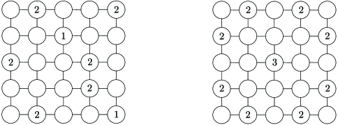
(a) a $\gamma_{R}$-function for RDP                                            (b) a $\gamma_{dR}$-function for DRDP

Figure 1: Example of RDP and DRDP on a $5\times 5$ grid graph (The dominating function value of the unlabelled vertex is $0$).

The double Roman domination number has been completely determined in paths and cycles [3], and has been shown to be linear-time solvable in trees [35] and $P_{4}$-free graphs [34]. However, for a general graph, it is NP-complete to determine whether a graph has a DRDF of weight at most $k$ [3]. Therefore, it is meaningful to obtain good upper and lower bounds for $\gamma_{dR}(G)$. Beeler et al. [7] studied the relationship between $\gamma_{dR}(G)$ and $\gamma(G)$ or $\gamma_{R}(G)$. They showed that $2\gamma(G)\leq\gamma_{dR}(G)\leq 3\gamma(G)$ and $\gamma_{R}(G)<\gamma_{dR}(G)\leq 2\gamma_{R}(G)$. Moreover, $\gamma_{dR}(T)\geq 2\gamma(T)+1$ for a non-trivial tree $T$. Later, Ahangar et al. [3] gave that a graph with maximum degree $\Delta$ satisfies $\gamma_{dR}(G)\geq\frac{2n}{\Delta}+\frac{\Delta-2}{\Delta}\gamma(G)$. Besides, there are some bounds for $\gamma_{dR}(G)$ in terms of order $n$, minimum degree $\delta$, maximum degree $\Delta$ and diameter $d$. Beeler et al. [7] proved that $\gamma_{dR}(G)\leq 5n/4$ for a connected graph $G$ with order $n\geq 3$, and characterized the graphs attaining this bound. In [33], Volkmann obtained the lower bound $\gamma_{dR}(G)\geq\lceil\frac{3n}{\Delta+1}\rceil$ for each nonempty graph $G$. Yue et al. [34] got the upper bounds $\gamma_{dR}(G)\leq 2n-2\Delta+1$ and $\gamma_{dR}(G)\leq\frac{3n(1+\ln{\frac{2(1+\delta)}{3}})}{1+\delta}$. They also showed that almost all graphs have double Roman domination number $\gamma_{dR}\leq n$. Recently, Anu et al. [6] found an upper bound with respect to order $n$ and diameter $d$, that is $d+1\leq\gamma_{dR}(G)\leq 2n-d$. In [6], Anu et al. showed that there is no relation between the double Roman domination number of a graph and its induced subgraph. Yue et al. [34] obtained that a graph with order $n\geq 3$ satisfies $8\leq\gamma_{dR}(G)+\gamma_{dR}(\overline{G})\leq 2n+3$ and characterized the graphs attaining these bounds. For other results on $\gamma_{dR}(G)$, we refer to [33, 25, 21, 5, 29].

However, for a specific graph, determining the exact value or designing approximation algorithms for the double Roman domination number has not been studied in the literature. For the RDP, several integer linear programming (ILP) formulations have been proposed by ReVelle and Rosing [30] and Ivanović [24]. Motivated by this, this paper will study the ILP formulations for the DRDP, and will also introduce several extra constraints to strengthen some ILP formulations. Additionally, an $H(2(\Delta+1))$-approximation algorithm for DRDP is proposed based on one ILP formulation.

The remainder of this paper is organized as follows. In Section 2, we propose two different ILP models for the DRDP. Two improved ILP formulations and two new alternative LP formulations are presented in Section 3. An approximation algorithm for DRDP is given in Section 4. Finally, we provide computational results in Section 5 and draw our conclusions in Section 6.

2 ILP models

In this section, we present two different ILP models for the DRDP. These models will be improved in Section 3 and experimentally evaluated in Section 5.

The first ILP model, called DRDP-1, uses three sets of binary variables. Specifically, for each vertex $v\in V$, we define

$$x_{v}=\left\{\begin{array}[]{ll}1,&\ f(v)=1\\ 0,&\ \text{otherwise}\\ \end{array}\right.\hskip 15.00002pty_{v}=\left\{\begin{array}[]{ll}1,&\ f(v)=2\\ 0,&\ \text{otherwise}\\ \end{array}\right.\hskip 15.00002ptz_{v}=\left\{\begin{array}[]{ll}1,&\ f(v)=3\\ 0,&\ \text{otherwise}\\ \end{array}.\right.$$

Then the DRDP can be formulated as follows:

$$\textbf{[DRDP-1]}\quad\min\quad \sum\limits_{v\in V}x_{v}+2\sum_{v\in V}y_{v}+3\sum_{v\in V}z_{v}$$ (1a)

s.t. $$x_{v}+y_{v}+z_{v}+\frac{1}{2}\sum_{u\in N(v)}y_{u}+\sum_{u\in N(v)}z_{u}\geq 1,\quad\forall\;v\in V$$ (1b)

$$\sum_{u\in N(v)}y_{u}+\sum_{u\in N(v)}z_{u}\geq x_{v},\quad\forall\;v\in V$$ (1c)

$$x_{v}+y_{v}+z_{v}\leq 1,\quad\forall\;v\in V$$ (1d)

$$x_{v},y_{v},z_{v}\in\{0,1\},\quad\forall\;v\in V$$ (1e)

The objective function value is given by (1a). Constraints (1b) ensure that if $f(v)=0$, then vertex $v$ must have at least two neighbors assigned $2$ under $f$ or at least one neighbor $u$ with $f(u)=3$. Constraints (1c) ensure that if $f(v)=1$, then vertex $v$ must have at least one neighbor $u$ with $f(u)\geq 2$. By constraints (1d), it establishes that every vertex is assigned with at most one value from the set $\{1,2,3\}$. The decision variables $x_{v},\ y_{v}$ and $z_{v}$ are set to be binary by constraints (1e).

The DRDP-1 formulation consists of $3|V|$ binary variables and $3|V|$ constraints. The following theorem shows that DRDP-1 indeed corresponds to the mathematical formulation of the double Roman domination problem.

Theorem 2.1.

The optimal objective function value of DRDP-1 formulation is equal to the double Roman domination number $\gamma_{dR}$.

Proof.  Let $S$ be the set of all the possible double Roman dominating functions and $T$ the set of all feasible solutions of DRDP-1 formulation. First we prove that there exists a bijection between $S$ and $T$.

For any double Roman dominating function $f\in S$, we construct a feasible solution $(\textbf{x},\textbf{y},\textbf{z})\in T\subseteq\{0,1\}^{3\times|V|}$:

1. if $f(v)=0$, then set $x_{v}=y_{v}=z_{v}=0$;

2. if $f(v)=1$, then set $x_{v}=1,y_{v}=z_{v}=0$;

3. if $f(v)=2$, then set $y_{v}=1,x_{v}=z_{v}=0$;

4. if $f(v)=3$, then set $z_{v}=1,x_{v}=y_{v}=0$.

Note that if $f(v)>0$, then one of $x_{v},y_{v},z_{v}$ equals one, so constraints (1b) are trivial. Otherwise, $v$ must have at least two neighbors assigned $2$ under $f$ or at least one neighbor $u$ with $f(u)=3$, which means there exist at least two vertices $u_{1},u_{2}\in N(v)$ satisfying $y_{u_{1}}=y_{u_{2}}=1$ or at least one vertex $u\in N(v)$ satisfying $z_{u}=1$ from our construction. Hence, constraints (1b) are also satisfied.

Consider constraints (1c). If $f(v)\neq 1$, then $x_{v}=0$, so constraints (1c) are trivial. Otherwise, $v$ must have at least one neighbor $u$ with $f(u)\geq 2$, which means $y_{u}=1$ or $z_{u}=1$ from our construction. Therefore, constraints (1c) hold as well.

Moreover, constraints (1d)–(1e) hold naturally from our construction. Consequently, we obtain an injection from $S$ to $T$.

For the other direction, given a feasible solution $(\textbf{x},\textbf{y},\textbf{z})\in T$, we construct a function $f:V\to\{0,1,2,3\}$ as follows:

1. if $x_{v}=y_{v}=z_{v}=0$, then set $f(v)=0$;

2. if $x_{v}=1,y_{v}=z_{v}=0$, then set $f(v)=1$;

3. if $y_{v}=1,x_{v}=z_{v}=0$, then set $f(v)=2$;

4. if $z_{v}=1,x_{v}=y_{v}=0$, then set $f(v)=3$.

Observe that constraints (1b) ensure that if $f(v)=0$, then vertex $v$ must have at least two neighbors assigned $2$ under $f$ or at least one neighbor $u$ with $f(u)=3$. Constraints (1c) guarantee that if $f(v)=1$, then vertex $v$ must have at least one neighbor $u$ with $f(u)\geq 2$. It follows that $f$ is a double Roman dominating function.

We have proved that there exists a bijection between $S$ and $T$. Since the objective function (1a) corresponds to the weight of a double Roman dominating function, then the optimal objective function value of DRDP-1 formulation is equal to the minimum weight among all the double Roman dominating functions, that is $\gamma_{dR}$.

$\square$

The second ILP model, called DRDP-2, follows the same idea as DRDP-1, apart from the definition of some binary variables. Similar as above, for each vertex $v\in V$, we define

$$p_{v}=\left\{\begin{array}[]{ll}1,&\ f(v)\geq 1\\ 0,&\ \text{otherwise}\\ \end{array}\right.\hskip 15.00002ptq_{v}=\left\{\begin{array}[]{ll}1,&\ f(v)\geq 2\\ 0,&\ \text{otherwise}\\ \end{array}\right.\hskip 15.00002ptr_{v}=\left\{\begin{array}[]{ll}1,&\ f(v)=3\\ 0,&\ \text{otherwise}\\ \end{array}.\right.$$

Then we can obtain another ILP model for DRDP:

$$\textbf{[DRDP-2]}\quad\min\quad \sum\limits_{v\in V}p_{v}+\sum_{v\in V}q_{v}+\sum_{v\in V}r_{v}$$ (2a)

s.t. $$p_{v}+\frac{1}{2}\sum_{u\in N(v)}q_{u}+\frac{1}{2}\sum_{u\in N(v)}r_{u}\geq 1,\quad\forall\;v\in V$$ (2b)

$$q_{v}+\sum_{u\in N(v)}q_{u}\geq p_{v},\quad\forall\;v\in V$$ (2c)

$$r_{v}\leq q_{v}\leq p_{v},\quad\forall\;v\in V$$ (2d)

$$p_{v},q_{v},r_{v}\in\{0,1\},\quad\forall\;v\in V$$ (2e)

The objective function value is given by (2a). Constraints (2b) ensure that if $f(v)=0$, then vertex $v$ must have at least two neighbors assigned $2$ under $f$ or at least one neighbor $u$ with $f(u)=3$. Constraints (2c) ensure that if $f(v)=1$, then vertex $v$ must have at least one neighbor $u$ with $f(u)\geq 2$. Constraints (2d) guarantee that the binary variables are well-defined. Again, the decision variables $p_{v},\ q_{v}$ and $r_{v}$ are preserved to be binary by constraints (2e).

The DRDP-2 formulation consists of $3|V|$ binary variables and $4|V|$ constraints. Similar to the previous arguments, we have the following theorem:

Theorem 2.2.

The optimal objective function value of DRDP-2 formulation is equal to the double Roman domination number $\gamma_{dR}$.

3 Alternative ILP models

In this section, we first improve the formulations introduced in Section 2, and then propose two alternative LP formulations.

3.1 Improved ILP formulations

To begin with, we state the following result proved by Beeler et al. [7].

Theorem 3.1 ([7]).

For any graph $G$, there exists a $\gamma_{dR}$-function of $G$ such that no vertex needs to be assigned the value $1$.

From Theorem 3.1, we can only consider the $\gamma_{dR}$-functions for which all vertices are assigned the value from the set $\{0,2,3\}$. Based on this, we substitute $0$ for $x_{v}$ in DRDP-1 to obtain the new ILP model DRDP-1^′.

$$\textbf{[DRDP-1${}^{\prime}$]}\quad\min\quad 2\sum_{v\in V}y_{v}+3\sum_{v\in V}z_{v}$$ (3a)

s.t. $$y_{v}+z_{v}+\frac{1}{2}\sum_{u\in N(v)}y_{u}+\sum_{u\in N(v)}z_{u}\geq 1,\quad\forall\;v\in V$$ (3b)

$$y_{v}+z_{v}\leq 1,\quad\forall\;v\in V$$ (3c)

$$y_{v},z_{v}\in\{0,1\},\quad\forall\;v\in V$$ (3d)

Using the same idea as the one in Theorem 2.1, we can obtain the following statement:

Theorem 3.2.

The optimal objective function value of DRDP-1^′ formulation is equal to the double Roman domination number $\gamma_{dR}$.

Proof.  Let $S$ be the set of all the possible double Roman dominating functions and $T$ the set of all feasible solutions of DRDP-1 formulation. Then let $S^{\prime}$ be the set of all the double Roman dominating functions that no vertex is assigned the value $1$. Clearly, $S^{\prime}\subseteq S$. Let $T^{\prime}$ be the set of all feasible solutions of DRDP-1^′ formulation. Note that for every feasible solution $(\textbf{y},\textbf{z})\in T^{\prime}$, one can obtain a feasible solution $(\overbrace{0,\ldots,0}^{n},\textbf{y},\textbf{z})\in T$. Since there exists a natural bijection between $T^{\prime}$ and the set $\{(\overbrace{0,\ldots,0}^{n},\textbf{y},\textbf{z})\ |\ (\textbf{y},\textbf{z})\in T^{\prime}\}\subseteq T$, $T^{\prime}\subseteq T$ holds. By Theorem 3.1, $S^{\prime}$ contains at least one $\gamma_{dR}$-function. It remains to show that there exists a bijection between $S^{\prime}$ and $T^{\prime}$ and that the objective function value of DRDP-1^′ corresponds to the weight of a double Roman dominating function in $S^{\prime}$, whose proof is similar to that in Theorem 2.1 (by excluding the cases $(b)$ and $(b^{\prime})$).

$\square$

Besides, we can substitute $q_{v}$ for $p_{v}$ in DRDP-2 by Theorem 3.1. Then we obtain another improved ILP model DRDP-2^′.

$$\textbf{[DRDP-2${}^{\prime}$]}\quad\min\quad 2\sum_{v\in V}q_{v}+\sum_{v\in V}r_{v}$$ (4a)

s.t. $$q_{v}+\frac{1}{2}\sum_{u\in N(v)}q_{u}+\frac{1}{2}\sum_{u\in N(v)}r_{u}\geq 1,\quad\forall\;v\in V$$ (4b)

$$r_{v}\leq q_{v},\quad\forall\;v\in V$$ (4c)

$$q_{v},r_{v}\in\{0,1\},\quad\forall\;v\in V$$ (4d)

Similar to Theorem 3.2, we deduce that,

Theorem 3.3.

The optimal objective function value of DRDP-2^′ formulation is equal to the double Roman domination number $\gamma_{dR}$.

Next, we explore some extra inequalities to strengthen the formulation DRDP-1^′. Note that for a $\gamma_{dR}$-function $f$ of graph $G$, the set $\{v\in V\ |\ f(v)\geq 2\}$ is a dominating set of $G$. Therefore, by the definition of $y_{v}$ and $z_{v}$, the sum $\sum_{v\in V}y_{v}+\sum_{v\in V}z_{v}$ is equal to the cardinality of the set $\{v\in V\ |\ f(v)\geq 2\}$, and we can conclude that the domination number $\gamma(G)$ is bounded by $\sum_{v\in V}y_{v}+\sum_{v\in V}z_{v}$. Since $\gamma(G)\geq\lceil n/(1+\Delta)\rceil$ [22], it is valid to write

$$\sum_{v\in V}y_{v}+\sum_{v\in V}z_{v}\geq\gamma(G)\geq\lceil\frac{n}{1+\Delta}\rceil.$$

Observing that for a $\gamma_{dR}$-function $f$ where all vertices are assigned the values from the set $\{0,2,3\}$, if we replace the function value $3$ by $2$ in $f$, the new function $f^{\prime}$ is a Roman dominating function (since $f$ is a double Roman dominating function, we know that every vertex $v\in V$ with $f^{\prime}(v)=0$ is adjacent to at least one vertex $u$ with $f^{\prime}(u)=2$). Thus the weight $2\sum_{v\in V}y_{v}+2\sum_{v\in V}z_{v}$ of the function $f^{\prime}$ is an upper bound for $\gamma_{R}(G)$, that is

$$2\sum_{v\in V}y_{v}+2\sum_{v\in V}z_{v}\geq\gamma_{R}(G).$$

There are some lower bounds for $\gamma_{R}(G)$ in [28]:

• $\gamma_{R}(G)\geq\lceil 2g/3\rceil$, when $G$ contains a cycle;

• $\gamma_{R}(G)\geq\lceil(d+2)/2\rceil$, when $G$ is connected;

• $\gamma_{R}(G)\geq 2\delta$, when $G$ is connected and $g\geq 5$;

• $\gamma_{R}(G)\geq 4(\delta-1)$, when $G$ is connected, $g\geq 6$ and $\delta\geq 2$;

• $\gamma_{R}(G)\geq 2\Delta$, when $G$ is connected, $g\geq 7$ and $\delta\geq 2$.

Therefore, a valid inequality for DRDP-1^′ is

$$2\sum_{v\in V}y_{v}+2\sum_{v\in V}z_{v}\geq L_{1},$$ (5)

where

$$L_{1}=\max\left\{2\cdot\lceil\frac{n}{1+\Delta}\rceil,\lceil\frac{2g}{3}\rceil\right\}.$$

For convenience, we use $g\geq a$ and $\delta\geq b$ to denote $\{G\ |\ g(G)\geq a\}$ and $\{G\ |\ \delta(G)\geq b\}$, respectively. For a family $\mathcal{A}$ of graphs, we define an indicator function $\textbf{1}_{\mathcal{A}}$ as follows:

$$\textbf{1}_{\mathcal{A}}(G)=\left\{\begin{array}[]{ll}1&\ \text{if}\ G\in\mathcal{A},\\ 0&\ \text{if}\ G\notin\mathcal{A}.\\ \end{array}\right.$$

Further, for a connected graph $G$, we can get a stronger inequality

$$2\sum_{v\in V}y_{v}+2\sum_{v\in V}z_{v}\geq L_{2}$$ (6)

where

$$L_{2}=\max\left\{2\cdot\lceil\frac{n}{1+\Delta}\rceil,\lceil\frac{d+2}{2}\rceil,\lceil\frac{2g}{3}\rceil,2\delta\cdot\textbf{1}_{g\geq 5},4(\delta-1)\cdot\textbf{1}_{g\geq 6\cap\delta\geq 2},2\Delta\cdot\textbf{1}_{g\geq 7\cap\delta\geq 2}\right\}.$$

Besides, there are some bounds for $\gamma_{dR}(G)$, which can also be used to derive extra inequalities. From [6, 33, 3], we know that $\gamma_{dR}(G)\geq\max\{d+1,\lceil 3n/(\Delta+1)\rceil,\lceil 2n/\Delta+(\Delta-2)\gamma(G)/\Delta\rceil\}$. So we can get

$$2\sum_{v\in V}y_{v}+3\sum_{v\in V}z_{v}\geq L_{3}$$ (7)

where

$$L_{3}=\max\left\{d+1,\lceil\frac{3n}{\Delta+1}\rceil,\lceil\frac{2n}{\Delta}+\frac{\Delta-2}{\Delta}\cdot\frac{n}{1+\Delta}\rceil\right\}.$$

Also, from [3, 7, 6, 34], we obtain that

1. $\gamma_{dR}(G)\leq\min\{2n-d,2n-2\Delta+1,3n(1+\ln\frac{2(1+\delta)}{3})/(1+\delta)\}$;

2. $\gamma_{dR}(G)\leq n$, when $\delta\geq 3$.

3. $\gamma_{dR}(G)\leq 5n/4$, when $G$ is a connected graph with order $n\geq 3$.

These upper bounds result in the constraint

$$2\sum_{v\in V}y_{v}+3\sum_{v\in V}z_{v}\leq U_{1}$$ (8)

where

$$U_{1}=\min\left\{2n-d,2n-2\Delta+1,n\cdot\textbf{1}_{\delta\geq 3}+3n\cdot(1-\textbf{1}_{\delta\geq 3}),\lfloor\frac{3n(1+\ln\frac{2(1+\delta)}{3})}{1+\delta}\rfloor\right\}.$$

Further, for a connected graph $G$ with order $n\geq 3$, the above inequality can be strengthened as

$$2\sum_{v\in V}y_{v}+3\sum_{v\in V}z_{v}\leq U_{2}$$ (9)

where

$$U_{2}=\min\left\{2n-d,2n-2\Delta+1,n\cdot\textbf{1}_{\delta\geq 3}+\lfloor\frac{5n}{4}\rfloor\cdot(1-\textbf{1}_{\delta\geq 3}),\lfloor\frac{3n(1+\ln\frac{2(1+\delta)}{3})}{1+\delta}\rfloor\right\}.$$

Similar as the above inequalities (5)–(7) and (8)–(9), we can also explore some extra constraints for the formulation DRDP-2^′. Especially, the sum $2\sum_{v\in V}q_{v}$ can be viewed as Roman dominating function’s weight, which is an upper bound for $\gamma_{R}(G)$. A series of extra inequalities for formulation (4a)–(4d) are listed as follows:

$$2\sum_{v\in V}q_{v}\geq L_{1},$$ (10)

$$2\sum_{v\in V}q_{v}+\sum_{v\in V}r_{v}\geq L_{2},$$ (11)

$$2\sum_{v\in V}q_{v}+\sum_{v\in V}r_{v}\leq U_{1}.$$ (12)

In addition, when $G$ is a connected graph with order $n\geq 3$, the above constraints (10) and (12) can be strengthened as

$$2\sum_{v\in V}q_{v}\geq L_{3},$$ (13)

and

$$2\sum_{v\in V}q_{v}+\sum_{v\in V}r_{v}\leq U_{2}.$$ (14)

We add the constraints (5)–(7) and (8)–(9) to DRDP-1^′ and denote the strengthened formulation by DRDP-1^′(+). Similarly, DRDP-2^′(+) stands for the new formulation obtained by adding constraints (10)–(13) and (12)–(14) into DRDP-2^′. In Section 5, we will explore the computational results for them.

3.2 Alternatives of the presented ILP formulations

In this section, we utilize the similar idea as the one in [24] to obtain two alternative LP formulations for DRDP and prove the equivalence between the new formulations and the previous ones.

The first formulation, denoted by DRDP-1^′′, is obtained from DRDP-1^′ by omitting constraints (3c).

$$\textbf{[DRDP-1${}^{\prime\prime}$]}\quad\min\quad 2\sum_{v\in V}y_{v}+3\sum_{v\in V}z_{v}$$ (15a)

s.t. $$y_{v}+z_{v}+\frac{1}{2}\sum_{u\in N(v)}y_{u}+\sum_{u\in N(v)}z_{u}\geq 1,\quad\forall\;v\in V$$ (15b)

$$y_{v},z_{v}\in\{0,1\},\quad\forall\;v\in V$$ (15c)

The following theorem proves the equivalence between DRDP-1^′′ and DRDP-1^′.

Theorem 3.4.

For any graph $G$, optimal objective function value of formulation (15a)–(15c) is equal to that of formulation (3a)–(3d).

Proof.  Let $V=\{1,\ldots,n\}$. The optimal objective function value of DRDP-1^′ and DRDP-1^′′ is denoted by $OPT_{1^{\prime}}$ and $OPT_{1^{\prime\prime}}$, respectively.

First, we prove $OPT_{1^{\prime\prime}}\geq OPT_{1^{\prime}}$. Note that an optimal solution to DRDP-1^′′ can be viewed as a vector $(\tilde{y}^{\prime\prime},\tilde{z}^{\prime\prime})\in\{0,1\}^{2n}$, where $\tilde{y}^{\prime\prime}=(y_{1}^{\prime\prime},\ldots,y_{n}^{\prime\prime})$, $\tilde{z}^{\prime\prime}=(z_{1}^{\prime\prime},\ldots,z_{n}^{\prime\prime})$. Based on this, we can divide $V$ into two disjoint subsets $V_{1}$ and $V_{2}$ such that

• $V_{1}=\{\;i\ |\ y_{i}^{\prime\prime}=0\ \text{or}\ z_{i}^{\prime\prime}=0\}$,

• $V_{2}=\{\;i\ |\ y_{i}^{\prime\prime}=1\ \text{and}\ z_{i}^{\prime\prime}=1\}$.

Then we define a new vector $(\tilde{y}^{\prime},\tilde{z}^{\prime})=(y_{1}^{\prime},\ldots,y_{n}^{\prime},z_{1}^{\prime},\ldots,z_{n}^{\prime})$ as follows:

$$y_{i}^{\prime}=\left\{\begin{aligned} y_{i}^{\prime\prime},\quad&\text{$\forall\;i\in V_{1}$},\\ 0,\ \quad&\text{$\forall\;i\in V_{2}$},\end{aligned}\right.~{}~{}~{}z_{i}^{\prime}=z_{i}^{\prime\prime},~{}\forall\;i\in V$$

Now, we prove that $(\tilde{y}^{\prime},\tilde{z}^{\prime})$ is a feasible solution to DRDP-1^′ formulation.

• For each $i\in V_{1}$, by the definition of variables $y_{i}^{\prime}$ and $z_{i}^{\prime}$ we know that $(y_{i}^{\prime},z_{i}^{\prime})=(y_{i}^{\prime\prime},z_{i}^{\prime\prime})$, so constraints (3b) and (3d) are satisfied. Further, from the definition of $V_{1}$, it follows that

  $$y_{i}^{\prime}+z_{i}^{\prime}=y_{i}^{\prime\prime}+z_{i}^{\prime\prime}\leq 1,\quad\forall\;i\in V_{1}$$

  that is, constraints (3c) are satisfied.

• For each $i\in V_{2}$, by the definition of variables $y_{i}^{\prime}$ and $z_{i}^{\prime}$, we obtain $(y_{i}^{\prime},z_{i}^{\prime})=(0,1)$. Then we can verify that constraints (3b)-(3d) are satisfied again:

  $$y_{i}^{\prime}+z_{i}^{\prime}+\frac{1}{2}\sum_{j\in N(i)}y_{j}^{\prime}+\sum_{j\in N(i)}z_{j}^{\prime}=0+1+\frac{1}{2}\sum_{j\in N(i)}y_{j}^{\prime}+\sum_{j\in N(i)}z_{j}^{\prime}\geq 1,\quad\forall\;i\in V_{2}$$

  $$y_{i}^{\prime}+z_{i}^{\prime}=0+1\leq 1,\quad\forall\;i\in V_{2}$$

  $$y_{i}^{\prime}=0\in\{0,1\},\quad z_{i}^{\prime}=1\in\{0,1\},\quad\forall\;i\in V_{2}$$

Therefore, an optimal solution $(\tilde{y}^{\prime\prime},\tilde{z}^{\prime\prime})$ to DRDP-1^′′ corresponds to a feasible solution $(\tilde{y}^{\prime},\tilde{z}^{\prime})$ to DRDP-1^′. It follows that

$$OPT_{1^{\prime\prime}} =2\sum_{i\in V}y_{i}^{\prime\prime}+3\sum_{i\in V}z_{i}^{\prime\prime}=2\sum_{i\in V_{1}}y_{i}^{\prime\prime}+3\sum_{i\in V_{1}}z_{i}^{\prime\prime}+2\sum_{i\in V_{2}}y_{i}^{\prime\prime}+3\sum_{i\in V_{2}}z_{i}^{\prime\prime}$$

$$=2\sum_{i\in V_{1}}y_{i}^{\prime\prime}+3\sum_{i\in V_{1}}z_{i}^{\prime\prime}+5|V_{2}|,$$

$$OPT_{1^{\prime}} \leq 2\sum_{i\in V}y_{i}^{\prime}+3\sum_{i\in V}z_{i}^{\prime}=2\sum_{i\in V_{1}}y_{i}^{\prime}+3\sum_{i\in V_{1}}z_{i}^{\prime}+2\sum_{i\in V_{2}}y_{i}^{\prime}+3\sum_{i\in V_{2}}z_{i}^{\prime}$$

$$=2\sum_{i\in V_{1}}y_{i}^{\prime\prime}+3\sum_{i\in V_{1}}z_{i}^{\prime\prime}+3|V_{2}|.$$

Hence, we get $OPT_{1^{\prime\prime}}\geq OPT_{1^{\prime}}$.

It remains to show that $OPT_{1^{\prime\prime}}\leq OPT_{1^{\prime}}$. Let $S^{\prime}$, $S^{\prime\prime}$ be the set of feasible solutions to DRDP-1^′ and DRDP-1^′′, respectively. Note that each feasible solution to DRDP-1^′ is also a feasible solution to DRDP-1^′′. Hence $S^{\prime}\subseteq S^{\prime\prime}$, which implies that

$$OPT_{1^{\prime\prime}}=\min_{S^{\prime\prime}}\left(2\sum_{i\in V}y_{i}+3\sum_{i\in V}z_{i}\right)\leq\min_{S^{\prime}}\left(2\sum_{i\in V}y_{i}+3\sum_{i\in V}z_{i}\right)=OPT_{1^{\prime}}.$$

This completes our proof.

$\square$

Next we prove that the binary variables $r_{v}$ in DRDP-2^′ formulation can be relaxed to non-negative real numbers, and thus we have the following MIP formulation DRDP-2^′′.

$$\textbf{[DRDP-2${}^{\prime\prime}$]}\quad\min\quad 2\sum_{v\in V}q_{v}+\sum_{v\in V}r_{v}$$ (16a)

s.t. $$q_{v}+\frac{1}{2}\sum_{u\in N(v)}q_{u}+\frac{1}{2}\sum_{u\in N(v)}r_{u}\geq 1,\quad\forall\;v\in V$$ (16b)

$$r_{v}\leq q_{v},\quad\forall\;v\in V$$ (16c)

$$q_{v}\in\{0,1\},\ r_{v}\in[0,+\infty),\quad\forall\;v\in V$$ (16d)

Theorem 3.5.

For any graph $G$, optimal objective function value of formulation (16a)–(16d) is equal to that of formulation (4a)–(4d).

Proof.  Let $V=\{1,\ldots,n\}$. We denote the optimal objective function value of DRDP-2^′ and DRDP-2^′′ by $OPT_{2^{\prime}}$ and $OPT_{2^{\prime\prime}}$, respectively.

Since the optimal objective function value of every relaxed minimization problem is less than or equal to that of the associated original problem, hence we get $OPT_{2^{\prime\prime}}\leq OPT_{2^{\prime}}$.

Therefore, we only need to prove that $OPT_{2^{\prime\prime}}\geq OPT_{2^{\prime}}$. Note that an optimal solution to DRDP-2^′′ can be viewed as a vector $(\tilde{q}^{\prime\prime},\tilde{r}^{\prime\prime})\in\{0,1\}^{2n}$, where $\tilde{q}^{\prime\prime}=(q_{1}^{\prime\prime},\ldots,q_{n}^{\prime\prime})$, $\tilde{r}^{\prime\prime}=(r_{1}^{\prime\prime},\ldots,r_{n}^{\prime\prime})$. And we define a new vector $(\tilde{q}^{\prime},\tilde{r}^{\prime})=(q_{1}^{\prime},\ldots,q_{n}^{\prime},r_{1}^{\prime},\ldots,r_{n}^{\prime})$ as follows:

$$q_{i}^{\prime}=q_{i}^{\prime\prime},\quad\forall i\in V$$

and

$$r_{i}^{\prime}=\left\{\begin{aligned} 0,\quad&\text{ $r_{i}^{\prime\prime}\in[0,1)$}\\ 1,\quad&\text{ $r_{i}^{\prime\prime}\in[1,+\infty)$}\end{aligned}\right.$$

Now we prove that $(\tilde{q}^{\prime},\tilde{r}^{\prime})$ is a feasible solution to DRDP-2^′ formulation. The variables $q_{i}^{\prime}$ and $r_{i}^{\prime}$ have binary values by definition, thus constraints (4d) hold. Note that

1. when $r_{i}^{\prime\prime}\in[0,1)$, $r_{i}^{\prime}=0\leq q_{i}^{\prime};$

2. when $r_{i}^{\prime\prime}\in[1,+\infty)$, $r_{i}^{\prime}=1\leq r_{i}^{\prime\prime}\leq q_{i}^{\prime\prime}=q_{i}^{\prime}$, where the second inequality follows from constraints (16c).

Therefore, constraints (4c) hold as well. Next we verify the validity of constraints (4b). Recall that for each $i\in V$, $q_{i}^{\prime\prime}+\frac{1}{2}\sum_{j\in N(i)}q_{j}^{\prime\prime}+\frac{1}{2}\sum_{j\in N(i)}r_{j}^{\prime\prime}\geq 1$ (constraints 16b) and $r_{i}^{\prime\prime}\leq q_{i}^{\prime\prime}$ (constraints 16c). We consider the following three cases:

1. $q_{i}^{\prime\prime}=1$ or there exist at least two different vertices $j_{1},j_{2}\in N(i)$ with $q_{j_{1}}^{\prime\prime}=q_{j_{2}}^{\prime\prime}=1$. Since $q_{j}^{\prime}=q_{j}^{\prime\prime}$ for each $j\in V$, constraints (4b) hold naturally for $q_{i}^{\prime}$ and $r_{i}^{\prime}$.

2. $q_{i}^{\prime\prime}=0$ and $q_{j}^{\prime\prime}=0$ for each $j\in N(i)$. By constraints (16c), we have $r_{j}^{\prime\prime}=0$ for each $j\in N(i)$, and hence $q_{i}^{\prime\prime}+\frac{1}{2}\sum_{j\in N(i)}q_{j}^{\prime\prime}+\frac{1}{2}\sum_{j\in N(i)}r_{j}^{\prime\prime}=0$, which contradicts the constraints (16b). Thus this case is impossible.

3. $q_{i}^{\prime\prime}=0$ and there exists a unique vertex $j_{0}\in N(i)$ such that $q_{j_{0}}^{\prime\prime}=1$. By constraints (16c), we get $\sum_{j\in N(i)\backslash j_{0}}r_{j}^{\prime\prime}=0$. From constraints (16b), it follows that $r_{j_{0}}^{\prime\prime}\geq 1$. So $q_{j_{0}}^{\prime}=r_{j_{0}}^{\prime}=1$, then constraints (4b) are satisfied for $q_{i}^{\prime}$ and $r_{i}^{\prime}$.

To sum up, constraints (4b)–(4d) are satisfied. Therefore, the vector $(\tilde{q}^{\prime},\tilde{r}^{\prime})$ is a feasible solution to DRDP-2^′ formulation, which implies

$$OPT_{2^{\prime}}\leq 2\sum_{i\in V}q_{i}^{\prime}+\sum_{i\in V}r_{i}^{\prime}\leq 2\sum_{i\in V}q_{i}^{\prime\prime}+\sum_{i\in V}r_{i}^{\prime\prime}=OPT_{2^{\prime\prime}}.$$

The second inequality follows from the definition of $(\tilde{q}^{\prime},\tilde{r}^{\prime})$. Thus we complete our proof.

$\square$

Remark. Actually, from constraints (16c), we can replace constraints (16d) by

$$q_{v}\in\{0,1\},\ r_{v}\in[0,1],\quad\forall\;v\in V$$

4 Approximation algorithm

In this section, we consider the approximation algorithm for the double Roman domination problem. We design a greedy algorithm based on the ILP formulation DRDP-1^′′. Firstly, consider the following integer programming of general covering problem:

$$\min \textbf{c}\cdot\textbf{x}$$ (17)

s.t. $$A\textbf{x}\geq\textbf{b}$$

$$\textbf{x}\in\{0,1\}^{2n}$$

Let $\textbf{x}=(y_{1},\ldots,y_{n},z_{1},\ldots,z_{n})^{T}$, $\textbf{c}=(\overbrace{2,\ldots,2}^{n},\overbrace{3,\ldots,3}^{n})$, $\textbf{b}=2\cdot\textbf{1}_{n}$, $A=\left[\begin{array}[]{cc}2I_{n}+A(G)&2(I_{n}+A(G))\end{array}\right]_{n\times 2n}$, where $I_{n}$ is a unit matrix of size $n$. Then we transform the DRDP-1^′′ formulation into a constrained general covering problem (17). Using the same method described in [17], we can design a greedy algorithm as follows:

Algorithm 1 Greedy

0:  a graph $G$

0:  $W_{1},W_{2}$

1:  $\textbf{x}\leftarrow\textbf{0},\ S\leftarrow\{1,\ldots,2n\}$

2:  while b $\neq$ 0 do

3:     $k\leftarrow\operatorname*{arg\,min}_{j\in S}\{c_{j}/\sum_{i=1}^{n}a_{ij}\}$

4:     $x_{k}\leftarrow 1$

5:     $S\leftarrow S-\{k\}$

6:     for $i=1$ to $n$ do

7:        $b_{i}\leftarrow b_{i}-a_{ik}$

8:        for $j\ \text{in}\ S$ do

9:           $a_{ij}\leftarrow\min\{a_{ij},b_{i}\}$

10:        end for

11:     end for

12:  end while

13:  $W_{1}\leftarrow\textbf{c}\cdot\textbf{x}$

14:  for $i=1$ to $n$ do

15:     if $x_{i}=x_{i+n}=1$ then

16:        $x_{i}\leftarrow 0$

17:     end if

18:  end for

19:  $W_{2}\leftarrow\textbf{c}\cdot\textbf{x}$

20:  return  $W_{1},W_{2}$

Theorem 4.1 ([17]).

If OPT is the optimal value of the above covering problem (17), $W_{1}$ is the value given by the greedy algorithm, then

$$\frac{W_{1}}{OPT}\leq H\left(\max_{1\leq j\leq 2n}\sum_{i=1}^{n}a_{ij}\right),$$

where $H(d)=\sum_{i=1}^{d}1/i$ is the first $d$ terms of the harmonic series.

By using Theorem 4.1, we can obtain that the greedy algorithm is an $H(2(\Delta+1))$-approximation algorithm for double Roman domination problem.

Corollary 4.2.

There exists an $H(2(\Delta+1))$-approximation algorithm for double Roman domination problem.

Proof.  Let OPT be the optimal objective function value of the formulation DRDP-1^′′. By applying algorithm 1, we have a feasible solution x satisfying the formulation DRDP-1^′′. Since $W_{2}\leq W_{1}$ (step $13$–$19$), with theorem 4.1, we have

$$\frac{W_{2}}{OPT}\leq\frac{W_{1}}{OPT}\leq H\left(\max_{1\leq j\leq 2n}\sum_{i=1}^{n}a_{ij}\right)=H(2(\Delta+1)),$$

Thus we complete our proof. $\square$

Note that $H(d)\leq 1+\ln d$, hence the approximation factor is bound by $O(\ln(2(\Delta+1)))$. Next we will show this approximation factor is best possible in some sense. Recall that $2\gamma(G)\leq\gamma_{dR}(G)\leq 3\gamma(G)$. We get the following result:

Lemma 4.3.

(1) If minimum dominating set problem can be approximated up to a factor of $\alpha$ in some graph class, then DRDP can be approximated up to a factor of $\frac{3}{2}\alpha$ in the same graph class.

(2) If DRDP can be approximated up to a factor of $\alpha$ in some graph class, then minimum dominating set problem can be approximated up to a factor of $\frac{3}{2}\alpha$ in the same graph class.

Proof.  (1) Let $S$ be the solution returned by some $\alpha$-approximation algorithm for minimum dominating set problem on input $G=(V,E)$. Then $|S|\leq\alpha\gamma(G)$. Let $f$ be the function such that $f(u)=3$ for each $u\in S$ and $f(u)=0$ for each $u\in V\setminus S$. It is easy to see that $f$ is a double Roman dominating function with weight $3|S|$. Thus $3|S|\leq 3\alpha\gamma(G)\leq\frac{3}{2}\alpha\gamma_{dR}(G)$.

(2) Let $f$ be the double Roman dominating function with $(V_{0},V_{1},V_{2},V_{3})$ returned by some $\alpha$-approximation algorithm for DRDP on input $G=(V,E)$, where $V_{i}=\{u\in V\ |\ f(u)=i\}$. Then $|V_{1}|+2|V_{2}|+3|V_{3}|\leq\alpha\gamma_{dR}(G)$. Obviously, $V_{2}\cup V_{3}$ forms a dominating set of $G$. So we get $|V_{2}|+|V_{3}|\leq\frac{1}{2}(|V_{1}|+2|V_{2}|+3|V_{3}|)\leq\frac{1}{2}\alpha\gamma_{dR}(G)\leq\frac{3}{2}\alpha\gamma(G)$.

$\square$

Lemma 4.4 ([14]).

Minimum dominating set problem cannot be approximated to within a factor of $(1-\varepsilon)\ln(n)$ in polynomial time for any constant $\varepsilon>0$ unless $NP\subseteq DTIME\left(n^{O(\log(\log(n)))}\right)$. The same results hold also in bipartite and split graphs (hence in chordal graphs, and in complements of chordal graphs as well).

Combining the above two lemmas, we can conclude that

Theorem 4.5.

DRDP cannot be approximated to within a factor of $\frac{2}{3}(1-\varepsilon)\ln(n)$ in polynomial time for any constant $\varepsilon>0$ unless $NP\subseteq DTIME\left(n^{O(\log(\log(n)))}\right)$. The same results hold also in bipartite and split graphs (hence in chordal graphs, and in complements of chordal graphs as well). $\square$

Remark. For Roman domination problem, if we use the new ILP formulation presented in [24] and set $\textbf{c}=(\overbrace{1,\ldots,1}^{n},\overbrace{2,\ldots,2}^{n})$, $A=\left[\begin{array}[]{c c}I_{n}&I_{n}+A(G)\end{array}\right]_{n\times 2n}$, $\textbf{b}=\textbf{1}_{n}$ in previous constrained general covering problem (17), then we can also apply the greedy algorithm 1 to Roman domination problem to obtain the approximate result. Hence we get

Corollary 4.6.

There exists an $H(\Delta+1)$-approximation algorithm for Roman domination problem.

5 Computational results

In this section, computational results which show effectiveness of the proposed DRDP formulations are summarized. All DRDP formulations were solved using CPLEX 12.8 optimization solvers. We use a Python package — “NetworkX”[36] to generate all graphs of different types and sizes and the greedy algorithm was carried out by Python 3.7.0. All computational experiments were performed on Intel(R) Core(TM) i5-4200U CPU $@$ 1.60GHz 2.30GHz with 8GB RAM under Windows 10 operating system.

For all computational experiments, we used grid graphs, random graphs generated by Erdős-Rényi $G(n,p)$ model and random trees which were chosen uniformly at random from the set of all trees on $n$ nodes. All the formulations posed above were applied exactly once to each problem instance. The computation time limit for the applications of CPLEX to each model was $3600$ seconds for each graph. The results are presented in numerical form in three tables: Table 2 contains the results for all grid graphs. The results for all random graphs and random trees are presented in Table 1 and Table 3, respectively. The first fourth columns of Table 2 indicate the name of the instances, the number of vertices ($|V|$), the number of edges ($|E|$) and the best solution value. For the Table 1, the first fourth columns are the number of vertices ($|V|$), the number of edges ($|E|$), the edge probability ($p$) to generate random graphs and the best solution value. The first three columns of Table 3 indicate the name of the instances, the number of vertices ($|V|$) and the optimal solution value. Each random graph and random tree with the same number of vertices has three different instances. These entries of three tables are followed by the results obtained using all the above formulations and approximation algorithm. For each formulation, the computation time required to prove optimality is given in seconds together with the number of nodes visited in the search tree or the number of iterations. For the greedy algorithm, results and time were presented in the table. More specifically, all formulations and the greedy algorithm are compared with each other and the best method of DRDP formulations (the least computation time) is marked in bold in each row. We use the sign “–” to show the instances where the optimal solution was not reached within 3600 seconds. For that in Table 1 and Table 2, the best results are shown for the corresponding case when 3600-second limit reaches.

Table 1 presents the computational results on random graphs. Considering the instances in Table 1, it can be seen that all six DRDP formulations perform better in dense graphs than in sparse graphs. And we can conclude that the computation time of the six models is closely related to the number of edges in a graph. Besides, comparing the performance of the six models, DRDP-1^′ and DRDP-1^′′ have better performance than others in general. Although we have added some extra constraints to DRDP-1^′ and DRDP-2^′, these new formulations DRDP-1^′(+) and DRDP-2^′(+) do not perform very well as we expect.

From Table 2, we observe that, on the whole, DRDP-1^′, DRDP-1^′(+) and DRDP-1^′′ perform better than the other formulations in grid graphs. In particular, for all instances with less than $200$ vertices, DRDP-1^′′ outperforms DRDP-1^′. This was to be expected, as the only difference in the two models is the elimination of a set of constraints. And DRDP-1^′(+) perform better than DRDP-1^′ in some degree. It can also be observed that DRDP-2^′ and DRDP-2^′′ are competitive with DRDP-1^′ and DRDP-1^′′ in the context of grid graphs with less than $200$ vertices.

When considering all instances together in Table 3, DRDP-1^′′ is the best-performing model on random trees, which is followed by DRDP-2^′. Note that the DRDP problem of tree is much easier than gird or random graph, since the six models can even handle tens of thousands of nodes within the time limit of 3600 seconds. Perhaps it is relevant to the complexity of the problem (One can construct a linear-time algorithm to compute the value of $\gamma_{dR}(T)$ for any tree $T$ [35]).

Furthermore, we can notice that the greedy algorithm was very competitive on grid and random graphs. However, this method performed much worse than any formulation in the case of random trees, especially when the tree’s order is very large. The main reason is probably that for random trees, this approximation algorithm does not sufficiently utilize the sparsity of matrix $A$.

6 Conclusions

In this paper, we investigated the double Roman domination problem. We first proposed two ILP formulations DRDP-1 and DRDP-2, and proved these models indeed correspond to the mathematical formulation of the double Roman domination problem. By Theorem 3.1, we can restrict our attention to the functions with no vertex assigned value 1, which leads to two improved models DRDP-1^′ and DRDP-2^′. Next, we explore some extra inequalities to strengthen the formulations DRDP-1^′ and DRDP-2^′. Furthermore, it was shown that constraints (3c) could be excluded from DRDP-1^′ and variables $z_{v}$ in DRDP-2^′ can be relaxed to non-negative real numbers. Thus we obtained two alternative formulations DRDP-1^′′ and DRDP-2^′′. Finally, we use one ILP formulation DRDP-1^′′ to give an $H(2(\Delta+1))$-approximation algorithm and provide an inapproximability result for this problem.

Our computational experiments were carried out on grid graphs and random graphs with up to $370$ vertices, and random trees up to $30000$ vertices. The results showed that DRDP-1^′ and DRDP-1^′′ outperformed the other formulations in most situations. Especially, DRDP-1^′′ is the best-performing model on random trees and the formulations with extra constraints did not perform very well like we expect. We also notice that the greedy algorithm was very competitive on grid and random graphs. We made several improvements (decrease some variables or add some extra constraints) in some formulations, but significant improvements in computational effort for strengthening those formulations were still expected. Given that optimization solver was not efficient in solving large sparse graphs, designing new exact methods or other approximation algorithms for DRDP is an interesting direction for future work.

Acknowledgments. Q. Cai is partially supported by National Natural Science Foundation of China (No. 11701297) and Open Project Foundation of Intelligent Information Processing Key Laboratory of Shanxi Province (No. CICIP2018005). Y. Shi and S. Yao are partially supported by National Natural Science Foundation of China (No. 11771221 and 11811540390), Natural Science Foundation of Tianjin, China (No. 17JCQNJC00300) and China-Slovenia bilateral project “Some topics in modern graph theory” (No. 12-6).

Table 1: Numerical results for grid graphs

Instance					DRDP-1				DRDP-1′				DRDP-1′(+)				DRDP-1′′				DRDP-2				DRDP-2′				DRDP-2′(+)				DRDP-2′′				Greedy
name	$|V|$	$|E|$	best		result	time	nodes		result	time	nodes		result	time	nodes		result	time	nodes		result	time	nodes		result	time	nodes		result	time	nodes		result	time	nodes		result	time
Grid05$\times$10	50	85	38		38	0.63	79		38	0.20	0		38	0.31	0		38	0.41	13		38	0.81	81		38	0.31	0		38	0.41	0		38	0.63	163		54	0.39
Grid05$\times$15	75	130	56		56	4.06	2528		56	1.20	630		56	1.73	550		56	0.72	201		56	1.7	2236		56	0.81	169		56	1.80	232		56	1.89	2821		80	1.07
Grid05$\times$20	100	175	74		74	29.44	15505		74	4.86	3348		74	3.41	2105		74	3.31	2576		74	38.48	56261		74	2.67	2773		74	3.02	2607		74	6.14	7440		105	2.19
Grid05$\times$25	125	220	92		92	200.39	87272		92	15.69	9631		92	14.50	5501		92	10.22	5210		92	173.11	89529		92	17.88	15051		92	32.27	29349		92	30.20	19124		134	4.21
Grid05$\times$30	150	265	110		110	–	–		110	235.53	73607		110	212.36	108141		110	135.11	84417		111	–	–		110	259.31	124201		110	220.97	115958		110	293.45	147695		160	7.35
Grid05$\times$35	175	310	128		129	–	–		128	507.59	142150		128	317.27	112420		128	353.78	92031		129	–	–		128	583.75	141225		128	537.42	178804		128	894.69	362089		185	12.33
Grid10$\times$10	100	180	72		72	22.94	18817		72	2.45	1418		72	2.03	796		72	1.25	461		72	16.19	14135		72	2.28	2335		72	2.56	2965		72	6.00	5554		90	1.78
Grid10$\times$15	150	275	106		106	738.36	140939		106	89.03	31426		106	76.48	32497		106	21.44	9335		106	493.26	160496		106	65.92	26816		106	180.01	144437		106	97.27	40352		138	6.10
Grid10$\times$20	200	370	140		141	–	–		140	1180.09	215452		140	2014.41	325629		140	3362.61	619175		140	–	–		141	–	–		140	2744.03	513429		139.99	–	–		182	13.98
Grid10$\times$25	250	465	174		175	–	–		174	–	–		174	–	–		175	–	–		174	–	–		174	–	–		175	–	–		175	–	–		220	25.90
Grid10$\times$30	300	560	208		209	–	–		211	–	–		209	–	–		208	–	–		208	–	–		209	–	–		210	–	–		210	–	–		268	44.43
Grid15$\times$15	225	420	155		155	–	–		155	1373.06	215668		155	1205.52	168916		155	1355.20	192572		156	–	–		155	1709.80	225916		155	2843.16	341775		155	1905.75	392388		194	19.21
Grid15$\times$20	300	565	204		205	–	–		204	–	–		204	–	–		204	–	–		205	–	–		205	–	–		205	–	–		204.99	–	–		258	42.19
Grid15$\times$25	375	710	254		254	–	–		254	–	–		259	–	–		254	–	–		253	–	–		254	–	–		254	–	–		254	–	–		323	79.26

Table 2: Numerical results for random graphs

Instance					DRDP-1				DRDP-1′				DRDP-1′(+)				DRDP-1′′				DRDP-2				DRDP-2′				DRDP-2′(+)				DRDP-2′′				Greedy
$|V|$	$|E|$	$p$	best		result	time	nodes		result	time	nodes		result	time	nodes		result	time	nodes		result	time	nodes		result	time	nodes		result	time	nodes		result	time	nodes		result	time
100	994	0.2	21		21	3.80	5724		21	2.22	5162		21	3.30	4827		21	2.42	5427		21	15.38	16799		21	6.08	8283		21	3.05	4994		21	19.52	32246		23	0.40
	2484	0.5	11		11	7.23	7519		11	4.45	8344		11	5.58	8356		11	4.53	8676		11	30.38	41450		11	6.70	8778		11	6.48	9196		11	256.86	302139		12	0.26
	3949	0.8	6		6	0.55	197		6	0.53	0		6	1.16	185		6	0.75	181		6	0.97	201		6	1.09	168		6	1.17	189		6	4.30	8249		6	0.17
150	2239	0.2	24		24	535.69	550441		24	1745.03	1987548		24	429.39	477868		24	3506.45	3619108		26	–	–		24	788.81	1176644		24	402.88	474078		23.99	–	–		27	0.89
	5596	0.5	11		11	73.67	54703		11	45.56	57470		11	31.25	31104		11	39.91	56138		11	422.19	338528		11	69.92	64322		11	29.16	18769		11	1523.83	2121825		12	0.45
	8903	0.8	6		6	1.97	298		6	1.56	302		6	2.19	291		6	1.44	298		6	2.83	221		6	2.39	267		6	2.44	212		6	16.48	12621		6	0.25
200	0	0.2	27		27	–	–		27	–	–		27	–	–		27	–	–		27	–	–		27	–	–		27	–	–		26.99	–	–		29	1.56
	9941	0.5	12		12	219.22	100591		12	139.25	93823		12	216.39	123961		12	122.53	100557		12	2159.20	986301		12	225.19	135567		12	239.94	107938		12	–	–		14	0.86
	15850	0.8	6		6	3.95	387		6	3.16	397		6	5.47	427		6	3.84	395		6	8.23	312		6	5.44	381		6	5.16	287		6	46.02	20269		9	0.58
250	6205	0.2	29		29	–	–		29	–	–		30	–	–		29	–	–		29	–	–		30	–	–		29	–	–		29	–	–		31	2.81
	15527	0.5	12		12	479.44	127117		12	294.11	122411		12	295.64	125937		12	253.73	127877		12	–	–		12	551.56	174352		12	500.33	143796		12	–	–		12	1.07
	24869	0.8	6		6	31.13	1906		6	9.83	2729		6	14.86	1743		6	7.08	995		6	70.42	3704		6	12.45	493		6	46.98	3059		6	142.36	37039		8	0.80
300	8948	0.2	30		30	–	–		30	–	–		30	–	–		30	–	–		30	–	–		30	–	–		30	–	–		30	–	–		30	4.51
	22393	0.5	12		12	1499.45	244786		12	802.33	217587		12	1319.98	349369		14	–	–		14	–	–		12	1470.81	252751		14	–	–		12	–	–		15	1.97
	35902	0.8	8		8	270.17	57352.00		8	113.47	37007		8	148.28	34773		8	99.38	37041		8	1289.20	128757		8	180.73	34821		8	223.06	31940		8	–	–		10	1.46

Table 3: Numerical results for random trees

Instance				DRDP-1			DRDP-1′			DRDP-1′(+)			DRDP-1′′			DRDP-2			DRDP-2′			DRDP-2′(+)			DRDP-2′′			Greedy
name	$|V|$	value		time	iterations		time	iterations		time	iterations		time	iterations		time	iterations		time	iterations		time	iterations		time	iterations		time	result
Tree-100-1	100	102		0.22	371		0.14	185		0.08	198		0.03	17		0.41	371		0.05	182		0.30	195		0.06	165		1.78	113
Tree-100-2		100		0.19	347		0.17	179		0.27	195		0.05	5		0.55	374		0.09	167		0.25	207		0.08	166		1.92	114
Tree-100-3		98		0.16	269		0.06	152		0.11	167		0.02	3		0.33	280		0.08	136		0.05	187		0.05	132		1.74	110
Tree-1000-1	1000	998		2.20	3258		0.52	1778		0.75	1926		0.11	20		1.55	3480		0.42	1654		0.47	1898		0.61	1576		1681.76	1149
Tree-1000-2		964		1.11	2993		0.78	1673		0.86	1774		0.08	16		1.16	3132		0.50	903		0.63	1706		0.88	1167		1523.83	1092
Tree-1000-3		982		1.30	3224		0.33	1719		0.80	1779		0.25	44		1.44	3318		0.53	1395		0.97	1763		0.73	1342		1628.42	1136
Tree-10000-1	10000	9838		15.84	32244		5.17	18151		7.25	1913		0.66	29		73.94	66361		3.17	14733		4.45	710		5.11	15042		–	–
Tree-10000-2		9833		13.73	32843		10.25	18082		7.44	1982		2.14	60		82.91	63080		3.52	15539		4.59	665		6.73	15183		–	–
Tree-10000-3		9868		26.83	32579		7.78	18064		7.09	2169		2.39	59		101.69	67826		5.28	15391		7.13	663		5.64	15166		–	–
Tree-20000-1	20000	19624		33.16	22924		7.81	4063		11.58	3807		1.16	123		97.83	70320		5.75	1317		10.23	1325		7.91	29821		–	–
Tree-20000-2		19622		30.64	22741		10.03	4205		13.83	3975		1.7	61		103.05	71581		5.61	1398		10.63	1510		8.03	30133		–	–
Tree-20000-3		19655		34.63	22315		8.08	4101		18.59	3924		3.19	828		95.89	70016		5.86	1352		13.05	1425		9.25	30120		–	–
Tree-30000-1	30000	29410		47.25	32731		12.08	5894		23.11	5817		2.25	393		161.22	103441		9.00	1996		19.27	2116		13.27	5500		–	–
Tree-30000-2		29309		44.33	31951		13.47	5816		21.70	5575		2.09	58		161.00	103398		9.58	2123		18.97	2225		13.52	5302		–	–
Tree-30000-3		29423		44.56	32812		19.19	5961		21.98	6098		2.27	458		149.20	102554		9.77	2024		17.56	2093		13.51	5532		–	–

References

- [1] H. A. Ahangar, J. Amjadi, M. Chellali, S. Nazari-Moghaddam and S. Sheikholeslami. Trees with double roman domination number twice the domination number plus two. Iran. J. Sci. Technol. Trans. A Sci., doi: https://doi.org/10.1007/s40995-018-0535-7, 2018.
- [2] H. A. Ahangar, A. Bahremandpour, S. Sheikholeslami, N. Soner, Z. Tahmasbzadehbaee and L. Volkmann. Maximal roman domination numbers in graphs. Util. Math., 103: 245–258, 2017.
- [3] H. A. Ahangar, M. Chellali and S. M. Sheikholeslami. On the double roman domination in graphs. Discrete Appl. Math., 232: 1–7, 2017.
- [4] H. A. Ahangar, T. W. Haynes and J. Valenzuela-Tripodoro. Mixed roman domination in graphs. Bull. Malays. Math. Sci. Soc., 40(4): 1443–1454, 2017.
- [5] J. Amjadi, S. Nazari-Moghaddam, S. M. Sheikholeslami and L. Volkmann. An upper bound on the double roman domination number. J. Combin. Optim., 36(1): 81–89, 2018.
- [6] V. Anu and A. Lakshmanan. Double roman domination number. Discrete Appl. Math., 244: 198–204, 2018.
- [7] R. A. Beeler, T. W. Haynes and S. T. Hedetniemi. Double roman domination. Discrete Appl. Math., 211: 23–29, 2016.
- [8] J. Bondy and U. Murty. Graph Therory, GTM 244. Springer-Verlag, New York, 2008.
- [9] E. Castorini, P. Nobili and C. Triki. Optimal routing and resource allocation in multi-hop wireless networks. Optim. Methods Softw., 23(4): 593–608, 2008.
- [10] J. Cecílio, J. Costa and P. Furtado. Survey on data routing in wireless sensor networks. In Wireless Sensor Network Technologies for the Information Explosion Era. Springer, Berlin, Heidelberg, 3–46, 2010.
- [11] E. W. Chambers, B. Kinnersley, N. Prince and D. B. West. Extremal problems for roman domination. SIAM J. Discrete Math., 23(3): 1575–1586, 2009.
- [12] W. A. Chaovalitwongse, T. Y. Berger-Wolf, B. Dasgupta and M. V. Ashley. Set covering approach for reconstruction of sibling relationships. Optim. Methods Softw., 22(1): 11–24, 2007.
- [13] M. Chellali, T. W. Haynes, S. T. Hedetniemi and A. A. McRae. Roman -domination. Discrete Appl. Math., 204: 22–28, 2016.
- [14] M. Chlebík and J. Chlebíková. Approximation hardness of dominating set problems in bounded degree graphs. Inform. and Comput., 206: 1264–1275, 2008.
- [15] E. J. Cockayne, P. A. Dreyer Jr, S. M. Hedetniemi and S. T. Hedetniemi. Roman domination in graphs. Discrete Math., 278(1-3): 11–22, 2004.
- [16] B. Das and V. Bharghavan. Routing in ad-hoc networks using minimum connected dominating sets. In Communications, 1997. ICC’97 Montreal, Towards the Knowledge Millennium. 1997 IEEE International Conference, 1: 376–380, 1997.
- [17] G. Dobson. Worst-case analysis of greedy heuristics for integer programming with nonnegative data. Math. Oper. Res., 7(4): 515–531, 1982.
- [18] P. A. Dreyer. Applications and variations of domination in graphs. Diss. Rutgers University, 2000.
- [19] W. Goddard and M. A. Henning. Independent domination in graphs: A survey and recent results. Discrete Math., 313(7): 839–854, 2013.
- [20] M. Hajibaba and N. J. Rad. Some notes on the roman domination number and italian domination number in graphs. In J. Phys. Conf. Ser., IOP Publishing, 890(1): 012123, 2017.
- [21] G. Hao, X. Chen and L. Volkmann. Double roman domination in digraphs. Bull. Malays. Math. Sci. Soc., doi: https://doi.org/10.1007/s40840-017-0582-9, 2017.
- [22] S. Hedetniemi, P. Slater and T. W. Haynes. Fundamentals of domination in graphs. CRC press, 2013.
- [23] M. A. Henning. A survey of selected recent results on total domination in graphs. Discrete Math., 309(1): 32–63, 2009.
- [24] M. Ivanović. Improved mixed integer linear programing formulations for roman domination problem. Publications de l’Institut Mathématique, 99(113): 51–58, 2016.
- [25] H. Jiang, P. Wu, Z. Shao and J.-B. Liu. The double roman domination numbers of generalized petersen graphs P(n,2). Preprints 2018, 2018070381, doi: https://doi.org/10.20944/preprints201807.0381.v1.
- [26] Y. Ma, Q. Cai and S. Yao. Integer linear programming models for the weighted total domination problem. Appl. Math. Comput., 358: 146–150, 2019.
- [27] H. Mercier, V. K. Bhargava and V. Tarokh. A survey of error-correcting codes for channels with symbol synchronization errors. IEEE Commun. Surv. Tutor, 12(1), 2010.
- [28] B. P. Mobaraky and S. M. Sheikholeslami. Bounds on Roman domination numbers of graphs. Matematički vesnik, 60(4): 247–253, 2008.
- [29] N. J. Rad and H. Rahbani. Some progress on the double roman domination in graphs. Discuss. Math. Graph Theory, doi: https://doi.org/10.7151/dmgt.2069, 2018.
- [30] C. S. ReVelle and K. E. Rosing. Defendens imperium romanum: a classical problem in military strategy. Amer. Math. Monthly, 107(7): 585–594, 2000.
- [31] I. Stewart. Defend the roman empire! Sci. Amer., 281(6): 136–138, 1999.
- [32] M. K. Tural, Maximal matching polytope in trees. Optim. Methods Softw., 31(3): 471–478, DOI: 10.1080/10556788.2015.1104679, 2016.
- [33] L. Volkmann. Double roman domination and domatic numbers of graphs. Commun. Comb. Optim., 3: 71–77, 2018.
- [34] J. Yue, M. Wei, M. Li and G. Liu. On the double roman domination of graphs. Appl. Math. Comput., 338: 669–675, 2018.
- [35] X. Zhang, Z. Li, H. Jiang and Z. Shao. Double roman domination in trees. Inform. Process. Lett., 134: 31–34, 2018.
- [36] A. A. Hagberg, D. A. Schult and P. J. Swart. Exploring network structure, dynamics, and function using NetworkX. in Proceedings of the 7th Python in Science Conference (SciPy2008), Gäel Varoquaux, Travis Vaught, and Jarrod Millman (Eds), (Pasadena, CA USA), 11–15, 2008.