Numerical Method for Nonlinear Optical Spectroscopies:
Ultrafast Ultrafast Spectroscopy

?abstractname?

We outline a novel numerical method, called Ultrafast Ultrafast ($\text{UF}^{2}$) spectroscopy, for calculating the $n^{\text{th}}$-order wavepackets required for calculating $n$-wave mixing signals. The method is simple to implement, and we demonstrate that it is computationally more efficient than other methods in a wide range of use cases. Resulting spectra are identical to those calculated using the standard response function formalism but with increased efficiency. The computational speed-ups of $\text{UF}^{2}$ come from (a) non-perturbative and costless propagation of the system time-evolution (b) numerical propagation only at times when perturbative optical pulses are non-zero and (c) use of the fast Fourier transform convolution algorithm for efficient numerical propagation. The simplicity of this formalism allows us to write a simple software package that is as easy to use and understand as the Feynman diagrams that organize the understanding of $n$-wave mixing processes.

I Introduction

Ultrafast nonlinear optical spectroscopies, in the perturbative light-matter limit, are powerful tools for elucidating details about the electronic structure and ultrafast dynamics of optically active systems. Interpreting such spectra often requires understanding what signals would be produced by a range of parametrized system Hamiltonians; one then seeks the best agreement with experimental results by varying system parameters such as energy levels, couplings, dephasing rates, and more. This kind of fitting, as in Ref. Perdomo-Ortiz et al., 2012, involves repeatedly rederiving the spectroscopic signals as system parameters change, which can be computationally expensive.

Simulations of nonlinear spectroscopies can be particularly challenging when the optical pulse durations are similar to relevant timescales in the system dynamics, especially when one must consider the pulses overlapping in time. The response-function formalism, described further below, provides a powerful way to understand nonlinear spectra and can be computationally efficient when considering the limit of impulsive optical pulses, those with durations shorter than any relevant system dynamics (Mukamel, 1999). For spectroscopies that rely on varying pulse durations, simulating those variations can be computationally expensive, limiting the range of systems and pulses one can study (Johnson et al., 2014).

The effects of finite pulse durations can be studied using perturbative (Engel, 1991; Meyer et al., 1999; Kato and Tanimura, 2001; Tsivlin, Meyer, and May, 2006; Cheng, Lee, and Fleming, 2007; Renziehausen, Marquetand, and Engel, 2009; Tanimura, 2012; Yuen-Zhou et al., 2014; Johnson et al., 2014; Bell, Conrad, and Siemens, 2015; Cina et al., 2016; Perlík, Hauer, and Šanda, 2017; Smallwood, Autry, and Cundiff, 2017; Do, Gelin, and Tan, 2017; Fetherolf and Berkelbach, 2017) and nonperturbative (Seidner, Stock, and Domcke, 1995; Mančal, Pisliakov, and Fleming, 2006; Seibt et al., 2009) methods (Domcke and Stock, 2007). Except in special cases, where the dynamics can be solved analytically (Perlík, Hauer, and Šanda, 2017; Smallwood, Autry, and Cundiff, 2017; Johnson et al., 2014; Cina et al., 2016), generic methods numerically solve the time-dependent Schrodinger equation to determine the system response and spectroscopic observables. In the frequently studied cases of electronic excitations coupled to vibrations or optical cavities, without breaking of chemical bonds, this integration is performed efficiently in a basis of electronic and vibrational/optical excitations, with respect to which the system Hamiltonian is generally highly sparse. The numerical integration is frequently performed using Runge-Kutta (RK) methods (Gelin, Egorova, and Domcke, 2005a, b, 2009a, 2009b; Tanimura and Maruyama, 1997; Yan, 2017; Fetherolf and Berkelbach, 2017), with other frequently used quantum dynamics packages using Adams-Bashforth (Johansson, Nation, and Nori, 2012) or Bulirsch-Stoer (Beck et al., 2000; Tsivlin, Meyer, and May, 2006) methods. An alternative approach, especially valuable in cases with bond breaking, where a continuum of vibrational states become relevant, uses a real- and Fourier-space pseudospectral representation of the wavefunction, frequently using the split-operator method to propagate the system dynamics (Feit, Fleck, and Steiger, 1982; Kosloff and Kosloff, 1983; Seibt et al., 2009; Renziehausen, Marquetand, and Engel, 2009).

There has recently been an increased interest in understanding the role of finite-pulse-duration effects in nonlinear spectroscopies, and there are several analytic methods for the propagation of the states required for calculating 4-wave mixing signals using particular shapes of finite pulses (Perlík, Hauer, and Šanda, 2017; Smallwood, Autry, and Cundiff, 2017; Johnson et al., 2014). Each of these methods assumes a particular, idealized pulse shape, such as a Gaussian (Smallwood, Autry, and Cundiff, 2017; Johnson et al., 2014) or Lorentzian (Perlík, Hauer, and Šanda, 2017) profile, and some include pulse overlap effects. These methods require that the eigenvalues and eigenvectors of the unperturbed system are known, allowing use of analytic results for the time-dependent perturbation theory (TDPT), which can be summed over all required states.

We present a complementary numerical technique we call Ultrafast Ultrafast ($\text{UF}^{2}$) spectroscopy, which combines features of the analytic and full numerical integration approaches. $\text{UF}^{2}$ assumes that the eigenvalues and eigenvectors of the unperturbed system are known but solves the integrals arising from TDPT numerically and can therefore treat arbitrary pulse shapes. $\text{UF}^{2}$ works for arbitrary perturbative order $n$, including pulse-overlap effects. It is a fast implementation of the standard results in perturbative nonlinear spectroscopy in the electric dipole approximation(Mukamel, 1999). The version we present here is for closed systems. It assumes that the system Hamiltonian is time-independent and has a finite relevant eigenbasis. When the pulses are finite, we perform the time propagation using the convolution theorem and the fast Fourier transform (FFT) and therefore benefit from the speed of the FFT. Working in the energy eigenbasis allows non-perturbative and costless time evolution of the system at times when the optical pulses are negligible, and $\text{UF}^{2}$ also solves the TDPT integrals during the pulses with such a small cost that they may not be computationally limiting even for reasonably large system Hamiltonians. These speed-ups give a dramatic improvement over algorithms that involve numerical integration of the wavefunctions or density matrices for each time-step.

In many cases, the limiting step of $\text{UF}^{2}$ is evaluating the expectation value of the dipole operator after the pulses have passed. The computational cost of $\text{UF}^{2}$ is dominated by the cost of matrix-vector multiplication, and so benefits from all the speed of linear algebra optimization on modern computers. As it relies on diagonalizing the Hamiltonian, it is clear that at some system size $\text{UF}^{2}$ will cease to be a competitive technique.

Conventional wisdom holds that diagonalization of the system Hamiltonian is too expensive to be worthwhile for prediction of nonlinear spectroscopies (Domcke and Stock, 2007). Especially for sparse matrices, as occur in e.g., vibronic systems, full or partial diagonalizations to attain the relevant eigenvalues and eigenvectors can be relatively efficient (Calvetti, Reichel, and Sorensen, 1994); more importantly, if one desires to study 2D spectra with a large number of different pulse delays, the diagonalization cost must be paid only once. Further, one can consider the effects of different pulse shapes, durations, and polarizations; various dipole coupling matrices; and thermal or rotational averaging, all without needing to rediagonalize. In many such cases, the diagonalization cost can be insignificant compared to the cost of generating the spectra, even for relatively large systems.

In Section II we derive the mathematical framework of $\text{UF}^{2}$, show how it is used, and describe some of the techniques that increase its efficiency. As with any perturbative technique, it is most efficient where the rotating wave approximation and phase matching can be assumed (see Section II.4), but it does not require these assumptions. In Section III we compare the computational cost of $\text{UF}^{2}$ to two alternatives: a Runge-Kutta-based direct propagation method, and a split-operator pseudospectral method, where we focus on example vibronic Hamiltonians. For sufficiently large systems, the direct propagation methods become more efficient than $\text{UF}^{2}$, but we show that for Hamiltonians with dimensions up to $O(10^{4})$, which includes a large number of widely studied cases, $\text{UF}^{2}$ outperforms the direct propagation methods. In the frequently studied case of systems with dimension less than 100, $\text{UF}^{2}$ can be two orders of magnitude faster than direct propagation methods. We demonstrate how $\text{UF}^{2}$ enables computationally efficient studies of the effects of varying system parameters and optical pulse shapes in Section IV, where we show transient absorption (TA) spectra for a system with a Hamiltonian of dimension 28 and demonstrate how $\text{UF}^{2}$ can be used to perform rapid parameter sweeps.

$\text{UF}^{2}$ is not only efficient but also easy and intuitive to use. The method is built around single-sided Feynman diagrams and their double-sided counterparts, which describe the perturbative pathways contributing to desired spectroscopic signals. Using the method is a simple process of translating a desired Feynman diagram into a set of iterative function calls. A python implementation of $\text{UF}^{2}$ is available for download at https://github.com/peterarose/ultrafastultrafast. This code includes examples of how to translate Feynman diagrams into the language of $\text{UF}^{2}$ and an example implementation that calculates TA spectra. It also contains a comparison Runge-Kutta integration method, usable with the same convenient interface.

II Algorithm

II.1 Overview

We begin with a Hamiltonian of the form

$$\hat{H}=\hat{H}_{0}+\hat{H}^{\prime}(t),$$ (1)

where the light-matter interaction in the electric-dipole approximation is

$$\hat{H}^{\prime}(t)=-\hat{\boldsymbol{\mu}}\cdot\boldsymbol{E}(t),$$ (2)

and is treated as a perturbation, where $\hat{\boldsymbol{\mu}}$ and $\boldsymbol{E}(t)$ are the dipole moment of the system and the external electric field, respectively. Bold face symbols indicate Cartesian vectors. $\hat{H}_{0}$ describes the material system (e.g., a molecule or quantum dot) and has eigenstates $\Ket{\phi}$ and eigenvalues $\hbar\omega_{\phi}$, which are assumed to be known (either analytically or numerically). Therefore the unitary time-evolution operator $\hat{U}_{0}(t-t_{0})=e^{-i\hat{H}_{0}(t-t_{0})/\hbar}$ is known. We assume that the set of eigenstates $\left\{\Ket{\phi}\right\}$ is finite, and that all relevant wavefunctions in this problem can be expressed using $N$ eigenfunctions as

$$\Ket{\psi(t)}=\sum_{\phi=1}^{N}e^{-i\omega_{\phi}t}c_{\phi}(t)\Ket{\phi}.$$ (3)

The electric dipole operator $\hat{\boldsymbol{\mu}}$ must be known in the eigenbasis of $\hat{H}_{0}$, where we define matrix elements as

$$\boldsymbol{\mu}_{\phi\phi^{\prime}}=\Bra{\phi}\hat{\boldsymbol{\mu}}\Ket{\phi^{\prime}}.$$

Note that only $\omega_{\phi}$ and $\boldsymbol{\mu}_{\phi\phi^{\prime}}$ are needed. The eigenfunctions themselves are unnecessary if $\boldsymbol{\mu}_{\phi\phi^{\prime}}$ can be calculated in some other way.

We describe the electric field classically as a sum of pulses, where each pulse is denoted by a lowercase letter starting from $a$. A typical 4-wave mixing signal would be calculated by using up to 4 pulses. We write the electric field as a sum over $L$ pulses,

$$\boldsymbol{E}(t)=\sum_{i=a,b,\dots,L}\boldsymbol{e}_{i}\varepsilon_{i}(t)+\boldsymbol{e}_{i}^{*}\varepsilon_{i}^{*}(t),$$

where $\boldsymbol{e}_{i}$ is the possibly complex polarization vector, and the amplitude $\varepsilon_{i}$ of each pulse is defined with envelope $A_{i}$, central frequency $\omega_{i}$, wavevector $\boldsymbol{k}_{i}$, and phase $\Theta_{i}$ as

$$\varepsilon_{i}(t)=A_{i}(t-t_{i})e^{-i\left[\omega_{i}(t-t_{i})-\boldsymbol{k}_{i}\cdot\boldsymbol{r}+\Theta_{i}\right]},$$ (4)

where $t_{i}$ is the arrival time of each pulse, and we define the Fourier transform of the pulse as

$$\tilde{\varepsilon}_{i}(\omega)=\frac{1}{\sqrt{2\pi}}\int_{-\infty}^{\infty}\mathrm{d}t\varepsilon_{i}(t)e^{i\omega t}.$$

Then the light-matter interaction is a sum over rotating ($\varepsilon_{i}$) and counter-rotating ($\varepsilon_{i}^{*}$) terms. We express these terms individually as

$$\hat{H}_{j^{(*)}}^{\prime}(t) =-\hat{\boldsymbol{\mu}}\cdot\boldsymbol{e}_{j}^{(*)}\varepsilon_{j}^{(*)}(t)$$ (5)

so that

$$\hat{H}^{\prime}(t)=\sum_{i=a,b,...,L}\hat{H}^{\prime}_{i}(t)+\hat{H}^{\prime}_{i^{*}}(t).$$ (6)

In general, 4-wave mixing signals are calculated from the third-order perturbed density matrix (Mukamel, 1999). For closed systems, as described here, we can decrease the computational complexity of the problem by calculating the necessary perturbed wavefunctions up to third-order. We expand the true time-dependent wavefunction using the usual perturbative expansion

$$\Ket{\psi(t)}=\Ket{\psi^{(0)}(t)}+\Ket{\psi^{(1)}(t)}+\Ket{\psi^{(2)}(t)}+...$$ (7)

where $\Ket{\psi^{(0)}(t)}$ is the initial time-independent (ignoring a trivial phase) state, and $\Ket{\psi^{(n)}(t)}$ is proportional to $\left(H^{\prime}(t)\right)^{n}$. $\text{UF}^{2}$ is a fast method for calculating $\Ket{\psi^{(n)}(t)}$. The total polarization field is

$$\boldsymbol{P}(t) =\Bra{\psi(t)}\hat{\boldsymbol{\mu}}\Ket{\psi(t)}$$

$$=\boldsymbol{P}^{(1)}(t)+\boldsymbol{P}^{(2)}(t)+\boldsymbol{P}^{(3)}(t)+...$$

To calculate $\boldsymbol{P}^{(n)}(t)$, we expand $\Ket{\psi(t)}$ using Eq. 7 and keep only terms proportional to $\left(\hat{H}^{\prime}(t)\right)^{n}$.(Peter Hamm, 2011) As an example, the $3^{\text{rd}}$-order polarization field is

$$\boldsymbol{P}^{(3)}(t)=\Bra{\psi^{(3)}(t)}\hat{\boldsymbol{\mu}}\Ket{\psi^{(0)}}+\Bra{\psi^{(2)}(t)}\hat{\boldsymbol{\mu}}\Ket{\psi^{(1)}}+c.c.$$

From $\boldsymbol{P}^{(3)}(t)$ any $3^{\text{rd}}$-order spectroscopic signal can be determined. $\boldsymbol{P}^{(3)}(t)$ is the material response coupled to emitted radiation after three optical interactions. In 2D photon echo (2DPE) spectroscopy, the response is due to a single interaction with each of 3 separate pulses, with arrival times $t_{a},t_{b},t_{c}$. The delay times between pulses are $t_{b}-t_{a}=\tau$ and $t_{c}-t_{b}=T$. The polarization field is therefore a function of $\tau$ and $T$: $\boldsymbol{P}^{(3)}(\tau,T;t)$. Typically the quantity of interest is actually the Fourier transform partner

$$\boldsymbol{P}^{(3)}(\tau,T;\omega)=\frac{1}{\sqrt{2\pi}}\int_{-\infty}^{\infty}\mathrm{d}t\boldsymbol{P}^{(3)}(\tau,T;t)e^{i\omega t}.$$

The polarization field produces a radiating optical field, which can be heterodyne detected using a fourth local oscillator (LO) pulse. For the case of the 2DPE rephasing signal, the desired signal is calculated as (Mukamel, 1999)

$$S_{\text{2D}}^{(3)}(\tau,T,\omega)=\text{Im}\left[\tilde{\varepsilon}_{LO}^{*}(\omega)\boldsymbol{e}_{LO}^{*}\cdot\boldsymbol{P}_{\text{2D}}^{(3)}(\tau,T;\omega)\right].$$ (8)

We derive $\text{UF}^{2}$ for the classic example given in Eq. 8. In Section IV, we show example TA spectra, which arise due to the interaction of two pulses, a pump and a probe, separated by the delay time $T$. In the TA case, the first two interactions happen with the pump pulse, and therefore $\tau=0$. The third interaction comes from the probe, which also acts as the local oscillator. TA calculations are thus a function of only two variables:

$$S_{\text{TA}}^{(3)}(T,\omega)=\text{Im}\left[\tilde{\varepsilon}_{\text{probe}}^{*}(\omega)\boldsymbol{e}_{\text{probe}}^{*}\cdot\boldsymbol{P}_{\text{TA}}^{(3)}(T,\omega)\right].$$ (9)

Returning to the more general case with $\tau$ varying, the canonical formula for calculating the third-order time-dependent polarization field is

$$P^{(3)}(\tau,T,t) =\iiint dt_{3}dt_{2}dt_{1}E(t-t_{3})E(t-t_{3}-t_{2}+T)$$

$$\times E(t-t_{3}-t_{2}-t_{1}+T+\tau)R(t_{1},t_{2},t_{3})$$ (10)

where we follow Mukamel and suppress the polarization of the fields, and $R(t_{1},t_{2},t_{3})$ is a material response function containing all of the factors arising from $\hat{H}_{0}$ and $\hat{\boldsymbol{\mu}}$ (Mukamel, 1999). This formulation separates the material properties ($\hat{H}_{0}$ and $\hat{\boldsymbol{\mu}}$) from the shapes of the electric fields. If the electric fields are impulsive (i.e., short compared with any system timescale), then the convolutions in Eq. 10 are trivial and spectral signals may be calculated directly from the response function.

In this paper we focus on the case where the shape of the electric field cannot be ignored, and therefore studying the response function alone is insufficient to predict, interpret or understand spectroscopic observables. The triple-nested convolutions of Eq. 10 are so costly that they are rarely carried out. We present a fast method for calculating the $n^{\text{th}}$-order wavefunctions, and thence the desired polarization $\boldsymbol{P}^{(n)}(t)$, with arbitrary pulse shapes. The wavepackets can be studied in conjunction with the signal, giving intuition for the underlying physics (Heller, 1981).

II.2 Derivation

We follow standard time-dependent perturbation theory by considering that at time $t_{0}$ the system begins in a time-independent state $\Ket{\psi^{(0)}(t_{0})}$, i.e., an eigenstate of $\hat{H}_{0}$. The perturbation $\hat{H}^{\prime}(t)$ is zero before $t_{0}$ and produces $\Ket{\psi(t)}$ as in Eq. 7, where $\Ket{\psi^{(n)}}$ has contributions proportional to $(\hat{H}^{\prime})^{n}$. Then the standard result has (Peter Hamm, 2011)

$$\Ket{\psi^{(n)}(t)} =-\frac{i}{\hbar}\int_{t_{0}}^{t}ds\hat{U}_{0}^{-1}(s-t)\hat{H}^{\prime}(s)\Ket{\psi^{(n-1)}(s)}.$$ (11)

Since $\Ket{\psi^{(0)}}$ is time-independent (up to a trivial phase), we are free to send $t_{0}\rightarrow-\infty$. We also substitute $t^{\prime}=t-s$ to arrive at

$$\Ket{\psi^{(n)}(t)}=-\frac{i}{\hbar}\int_{0}^{\infty}dt^{\prime}\hat{U}_{0}(t^{\prime})\hat{H}^{\prime}(t-t^{\prime})\Ket{\psi^{(n-1)}(t-t^{\prime})}.$$

Using the decomposition of $\hat{H}^{\prime}(t)$ in Eq. 6, we define $\Ket{\psi^{(n)}(t)}$ as a sum over $2L$ terms

$$\Ket{\psi^{(n)}(t)} =\sum_{j=a,b,\dots,L}\left(\hat{K}_{j}+\hat{K}_{j^{*}}\right)\Ket{\psi^{(n-1)}(t)},$$

where

$$\hat{K}_{j^{(*)}}=-\frac{i}{\hbar}\int_{0}^{\infty}dt^{\prime}\hat{U}_{0}(t^{\prime})\hat{H}^{\prime}_{j^{(*)}}(t-t^{\prime}).$$

A small rearrangement of terms allows us to perform this integral numerically much more quickly:

$$\hat{K}_{j^{(*)}}=-\frac{i}{\hbar}\hat{U}_{0}(t)\int_{0}^{\infty}dt^{\prime}\hat{U}_{0}^{-1}(t-t^{\prime})\hat{H}^{\prime}_{j^{(*)}}(t-t^{\prime}).$$ (12)

Most spectroscopic signals are not calculated using the full perturbative wavefunction $\Ket{\psi^{(n)}(t)}$, because only specific pathways give nonzero contributions, which are visualized using Feynman diagrams, as in Fig. 1.(Mukamel, 1999) Each operator $\hat{K}_{j^{(*)}}$ represents a single interaction arrow in a Feynman diagram, as in Fig. 2. $\text{UF}^{2}$ calculates the wavefunctions contributing to each diagram separately. For example, as shown in Fig. 1, the excited state absorption (ESA) contribution requires two wavefunctions that we label $\Ket{\psi_{bc}(t)}\equiv\hat{K}_{c}\hat{K}_{b}\Ket{\psi^{(0)}}$ and $\Ket{\psi_{a}(t)}\equiv\hat{K}_{a}\Ket{\psi^{(0)}}$.

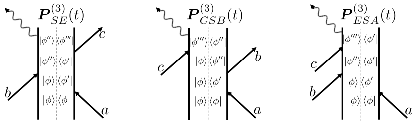
?figurename? 1: From left to right, stimulated emission (SE), ground-state bleach (GSB), and excited-state absorption (ESA) double-sided Feynman diagrams for the rephasing 2D photon echo signal. The dashed lines down the centers of each diagram emphasize that the ket and bra evolve independently for closed systems. We calculate the left and right sides of the diagram separately. These are the only three diagrams that contribute to the rephasing signal when the pulses are well-separated in time, though additional diagrams must be considered when pulses overlap.

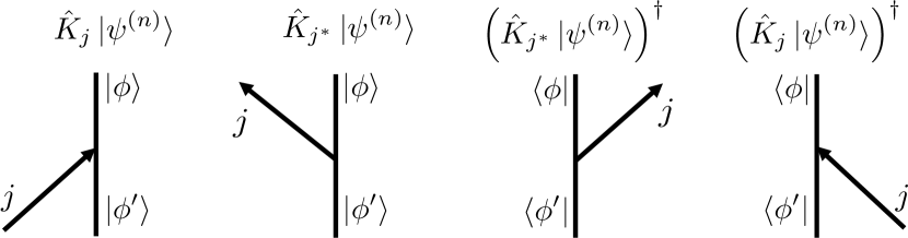
?figurename? 2: Building blocks of Feynman diagrams for the interaction with optical pulse $j$. The left two diagrams are for kets and the right two are for bras. Time moves from bottom to top, as the system begins in a linear combination of states $\Ket{\phi^{\prime}}$, and evolves to a linear combination of states $\Ket{\phi}$. The arrow sloping up to the right is a contribution of the operator $K_{j}$, and the arrow sloping up to the left is a contribution of the operator $K_{j^{*}}$.

Following Eq. 3, we write

$$\Ket{\psi_{p}(t)}=\sum_{\phi^{\prime}}e^{-i\omega_{\phi^{\prime}}t}c_{\phi^{\prime},p}(t)\Ket{\phi^{\prime}},$$

where $p$ can be a multi-index, such as $ac^{*}$. Then we use Eqs. 5 and 12 to write

$$\Ket{\psi_{pj^{(*)}}(t)} \equiv\hat{K}_{j^{(*)}}\Ket{\psi_{p}(t)}$$

$$=\frac{i}{\hbar}\hat{U}_{0}(t)\int_{0}^{\infty}dt^{\prime}\hat{U}_{0}^{-1}(t-t^{\prime})\sum_{\phi}\Ket{\phi}\Bra{\phi}\left(\hat{\boldsymbol{\mu}}\cdot\boldsymbol{e}_{j}^{(*)}\varepsilon_{j}^{(*)}(t-t^{\prime})\right)\sum_{\phi^{\prime}}e^{-i\omega_{\phi^{\prime}}(t-t^{\prime})}c_{\phi^{\prime},p}(t-t^{\prime})\Ket{\phi^{\prime}}$$ (13)

$$=\sum_{\phi}e^{-i\omega_{\phi}t}\Ket{\phi}\frac{i}{\hbar}\int_{-\infty}^{\infty}dt^{\prime}\theta(t^{\prime})\underbrace{e^{i\omega_{\phi}(t-t^{\prime})}\sum_{\phi^{\prime}}\left(\boldsymbol{\mu}_{\phi\phi^{\prime}}\cdot\boldsymbol{e}_{j}^{(*)}\varepsilon_{j}^{(*)}(t-t^{\prime})\right)e^{-i\omega_{\phi^{\prime}}(t-t^{\prime})}c_{\phi^{\prime},p}(t-t^{\prime})}_{y_{\phi}(t-t^{\prime})},$$ (14)

where $\theta(t)$ is the unit step function. We rewrite Eq. 14 as

$$\Ket{\psi_{pj^{(*)}}(t)}=\sum_{\phi}e^{-i\omega_{\phi}t}\Ket{\phi}\underbrace{\frac{i}{\hbar}\left[\theta*y_{\phi}\right](t)}_{c_{\phi,pj^{(*)}}(t)},$$ (15)

where

$$\left[x*y\right](t)=\int_{-\infty}^{\infty}dt^{\prime}x(t^{\prime})y(t-t^{\prime})$$

is a convolution. Thus we arrive at a compact description of the coefficients $c_{\phi,pj^{(*)}}(t)$.

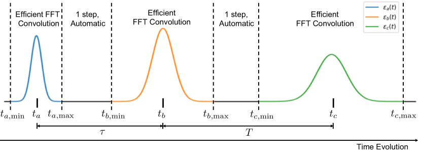
?figurename? 3: Sequence of three pulse envelopes, as would be used in a rephasing 2DPE experiment, showing the time intervals $(t_{j,\min},t_{j,\max})$ during which the pulses are non-negligible. $\text{UF}^{2}$ only performs time propagations during these time periods, using efficient FFT convolutions. At other times, the system time evolution operator $\hat{U}_{0}$ gives exact time evolution.

If we make the physical assumption that the incident pulse is localized in time, i.e., $\varepsilon_{i}(t)$ is negligible for $t<t_{j,\min}$ or $t>t_{j,\max}$, then it is also true that $y_{\phi,\alpha j^{(*)}}(t)$ is negligible when $t<t_{j,\min}$ or $t>t_{j,\max}$. This assumption implies that

$$c_{\phi,pj^{(*)}}(t)=\begin{cases}0&t<t_{j,\min}\\ r_{\phi}(t)&t_{j,\min}<t<t_{j,\max}\\ C_{\phi}&t>t_{j,\max}\end{cases}.$$ (16)

Therefore, we need only calculate this convolution for $t_{j,\min}<t<t_{j,\max}$ (see Fig. 3). Note that without the rearrangement of Eq. 12, the convolution in Eq. 15 would be more difficult to evaluate numerically because the functions $c_{\phi,pj^{(*)}}(t)$ would include the phase factor $e^{-i\omega_{\phi}t}$ even after $t_{j,\text{max}}$ and thus not be constant. This trivial definitional difference when working symbolically makes a large difference when working numerically,and constitutes one of the primary novel contributions of this work.

While Eq. 14 is a rearrangement of the response function formalism, and forms of it appear in References Seibt et al., 2009; Yuen-Zhou et al., 2014; Smallwood, Autry, and Cundiff, 2017; Perlík, Hauer, and Šanda, 2017, the integral in Eq. 14 is usually incorporated into the numerical propagation in direct propagation methods (Engel, 1991; Meyer et al., 1999; Seibt et al., 2009; Renziehausen, Marquetand, and Engel, 2009; Yuen-Zhou et al., 2014), or is handled analytically (Bell, Conrad, and Siemens, 2015; Smallwood, Autry, and Cundiff, 2017; Perlík, Hauer, and Šanda, 2017; Do, Gelin, and Tan, 2017). By expressing this integral as a linear convolution over a small set of points, we are able to include the effects of pulse shapes at a modest cost, as shown in Appendix A, depending on the desired signal accuracy.

Physically, we only need to solve for the time dependence due to the interaction while the pulse is non-zero. The rest of the time-dependence is contained entirely in $\hat{H}_{0}$, and is therefore known exactly. This realization drastically reduces the computational cost of $\text{UF}^{2}$ compared to techniques that must use time-stepping for both the system dynamics and the perturbation. We solve for the function $r_{\phi}(t)$ in Eq. 16 numerically using the convolution theorem and FFT. With Gaussian pulse shapes of any duration, for convergence of spectroscopic signals to a tolerance of 1%, we find that 20-40 points is sufficient for calculating each convolution in Eq. 15. With such a small number of required points, the evaluation of the dipole expectation value $\vec{P}(t)=<\psi|\hat{\mu}|\psi>$ is as expensive as the propagation, as we detail in Appendix A.

Translating the operators $K_{j^{(*)}}$ into computational algorithms is straightforward. We discretize the time interval $(t_{j,\text{min}},t_{j,\text{max}})$ to have $M$ equally spaced points with spacing $dt$, which must be small enough to resolve the pulses. Therefore, the wavefunctions that give rise to the ESA signal are calculated in three steps:

1. Calculate $\Ket{\psi_{a}(t)}=\hat{K}_{a}\Ket{\psi^{(0)}}$,

2. Calculate $\Ket{\psi_{b}(t)}=\hat{K}_{b}\Ket{\psi^{(0)}}$ for fixed $\tau$,

3. Calculate $\Ket{\psi_{bc}(t)}=\hat{K}_{c}\Ket{\psi_{b}(t)}$ for fixed $T$.

The polarization field is then

$$\boldsymbol{P}_{ESA}^{(3)}(t)|_{\tau,T}=\Bra{\psi_{a}(t)}\hat{\boldsymbol{\mu}}\Ket{\psi_{bc}(t)}|_{\tau,T}.$$ (17)

This process is repeated for all $\tau$ and $T$ of interest.

We demonstrate how this conceptual procedure is implemented using the syntax of $\text{UF}^{2}$.

⬇

psi_a = uf2.up(uf2.psi0,pulse_number = 0)

psi_b = uf2.up(uf2.psi0,pulse_number = 1)

psi_bc = uf2.up(psi_b,pulse_number = 2)

P_ESA = uf2.dipole_expectation(psi_a,psi_bc)

S_ESA = uf2.polarization_to_signal(P_ESA)

In the syntax of $\text{UF}^{2}$, pulse $a$ is pulse 0, pulse $b$ is pulse 1, etc., and the up and down methods implement $K_{j}$ and $K_{j^{*}}$, respectively. This snippet is adapted from the Jupyter notebook Example.ipynb included with the source code.

One of the strengths of $\text{UF}^{2}$ is that the user interacts with it by translating Feynman diagrams into nested calls to the $\hat{K}_{i^{(*)}}$ functions. The goal of this algorithm is to make calculating spectra as easy as writing down Feynman diagrams. We have used $3^{\text{rd}}$-order diagrams for the derivation because they are the most familiar, but calculating arbitrary order diagrams is just as straightforward. $\text{UF}^{2}$ is therefore easy to use and avoids the necessity of first writing out lengthy symbolic expressions for each diagram and translating each expression into code. $\text{UF}^{2}$ can also be used in the impulsive limit to calculate response functions, allowing this ease of use to be applied to the study of response functions as well.

II.3 Optical dephasing

For closed systems, $\boldsymbol{P}^{(n)}(t)$ oscillates for all time after the $n$ optical interactions. This undamped oscillation is unphysical. In order to include optical dephasing in general, we would need to solve for the third-order density matrix, $\rho^{(3)}(t)$, instead of the wavepackets. In order to include optical dephasing in our polarization signals, we convolve $\tilde{\boldsymbol{P}}^{(n)}(\omega)$ with a lineshape function, as in Ref. Seibt et al., 2009. Whereas that work used a Gaussian shape to model inhomogeneous broadening, in the examples below we use a Lorentzian lineshape to model homogeneous broadening due to an exponential dephasing.

II.4 Useful standard approximations

The derivations in Section II.2 do not require the rotating wave approximation (RWA) or phase matching. However, these approximations significantly reduce the cost of the calculations, as in all perturbative spectroscopies.(Cho, 2009; Peter Hamm, 2011; Mukamel, 1999) In the RWA, only one of either the rotating or counter-rotating terms of Eq. 6 contributes to an interaction.(Peter Hamm, 2011) Since $\Ket{\psi^{(n)}(t)}\propto\left(\hat{H}^{\prime}(t)\right)^{n}$, the $n^{\text{th}}$-order wavefunction is composed of $(2L)^{n}$ terms. The standard RWA and phase-matching conditions reduce the number of terms relevant to spectroscopic signals. The RWA is valid in the limit that the pulse durations are long compared to the optical carrier frequencies, which are roughly degenerate with the optical energy gap of $\hat{H}_{0}$. If the material system is dispersed over a volume much larger than the wavelength of the light then the phase-matching condition ensures that signal fields will be produced only in directions corresponding to sums and differences of wavevectors of the optical pulses (Mukamel, 1999). For example Fig. 1 shows the signals produced in the rephasing direction ($-\boldsymbol{k}_{a}+\boldsymbol{k}_{b}+\boldsymbol{k}_{c}$) of 2D photon echo (2DPE) spectroscopy.

In addition to reducing the number of relevant diagrams, the RWA speeds up calculations because we do not need to keep track of the optical carrier frequency. This advantage is significant because $\text{UF}^{2}$ performs calculations using $M$ time points with spacing $dt$ from $t_{j,\min}$ to $t_{j,\max}$. In the RWA, we set the optical carrier frequency to 0, and therefore $dt$ only needs to resolve the pulse envelope and not the carrier frequency.

II.5 Efficiency improvements

We increase the efficiency of $\text{UF}^{2}$ by decreasing the required dimensionality of the Hilbert space from the full size, $N_{\text{total}}$, to a compressed subspace of dimension $N_{c}$, over which the sums in Eq. 14 run. We perform the reduction from $N_{\text{total}}$ to $N_{c}$ before running any propagations by determining which elements of the dipole operator $\hat{\boldsymbol{\mu}}$ will not contribute appreciably to the calculation and ignoring them. We can prune the required set of states in two ways. First, many systems have elements $\boldsymbol{\mu}_{\phi^{\prime}\phi}\approx 0$. Second, we determine which energetic transitions will not be allowed by the electric field shape.

We use Bessel’s inequality to define which states $\Ket{\phi^{\prime}}$ are important in order to resolve $\boldsymbol{\mu}_{\phi^{\prime}\phi}$ accurately. If we begin in the eigenstate $\Ket{\phi}$, one interaction with the dipole operator (as occurs in each application of $K_{j^{(*)}}$) yields the state

$$\Ket{\Phi} =\hat{\boldsymbol{\mu}}\Ket{\phi}=\sum_{\phi^{\prime}=1}^{N_{\text{total}}}\boldsymbol{\mu}_{\phi^{\prime}\phi}\Ket{\phi^{\prime}}.$$

We seek to restrict the sum to the smallest number of terms without significantly altering the norm of this state, which implies that we have captured all of the physically relevant states. We write the norm of $\Ket{\Phi}$ as

$$\Braket{\Phi}{\Phi}=\sum_{\phi^{\prime}=1}^{N_{\text{total}}}|\boldsymbol{\mu}_{\phi^{\prime}\phi}|^{2}=\Bra{\phi}\hat{\boldsymbol{\mu}}^{2}\Ket{\phi}=\left(\boldsymbol{\mu}^{2}\right)_{\phi\phi}.$$

We find the smallest set of states, $N_{c}$, such that

$$\frac{\left(\boldsymbol{\mu}^{2}\right)_{\phi\phi}-\sum^{{}^{\prime}}|\boldsymbol{\mu}_{\phi\phi^{\prime}}|^{2}}{\left(\boldsymbol{\mu}^{2}\right)_{\phi\phi}}>1-\epsilon,$$ (18)

for small $\epsilon$, where $\sum^{\prime}$ represents the restricted sum over the required $N_{c}$ states. We perform this analysis for all required states $\Ket{\phi}$.

We make this concept concrete by giving an example using the non-rephasing ground state bleach signal, which is not included in Fig. 1. The polarization field produced by that diagram is $\boldsymbol{P}_{GSB,NR}^{(3)}(t)=\Bra{\psi^{(0)}}\boldsymbol{\mu}\Ket{\psi_{ab^{*}c}(t)}$. If we begin, say, in the state $\Ket{\psi^{(0)}}=\Ket{1}$, the lowest energy eigenstate of $\hat{H}_{0}$, then we must determine the smallest number of states, $N_{c}^{(1)}$, that satisfy Eq. 18 for $\phi=1$. Then we know before calculating Eq. 14 that $\Ket{\psi_{a}(t)}=\sum c_{\phi,a}(t)\Ket{\phi}$ will be composed of $N_{c}^{(1)}$ terms. To find the states required to describe $\Ket{\psi_{ab^{*}}}$, we use Eq. 18 for each of the $N_{c}^{(1)}$ states needed for $\Ket{\psi_{a}(t)}$, which gives a new set of $N_{c}^{(2)}$ states, where the superscript indicates the number of times $\hat{\mu}$ has been applied to the initial state.

The next obvious step is to use Eq. 18 for each of those $N_{c}^{(2)}$ states, but that step is actually unnecessary. Such an analysis would allow us to determine the $N_{c}^{(3)}$ states required to resolve $\Ket{\psi_{ab^{*}c}(t)}$. However, the final signal depends upon $\Bra{\psi^{(0)}}\boldsymbol{\mu}\Ket{\psi_{ab^{*}c}(t)}$, and therefore the only components of $\Ket{\psi_{ab^{*}c}(t)}$ that matter spectroscopically are those that overlap with $\boldsymbol{\mu}\Ket{\psi^{(0)}}$. These are precisely the $N_{c}^{(1)}$ states we determined in the first step of this process. Therefore we only need the same $N_{c}^{(1)}$ states when calculating $\Ket{\psi_{ab^{*}c}(t)}$.

For many systems relevant to optical spectroscopy, there are well-separated manifolds of states with 0, 1, 2, etc. electronic excitations. When there are well-separated manifolds, the RWA allows a further reduction to the relevant size $N_{c}$. In the same non-rephasing GSB example, $\Ket{\psi_{a}(t)}$ is in the singly excited manifold (SEM), and $\hat{\mu}\Ket{\psi_{a}(t)}$ has components in both the ground state manifold (GSM) and the doubly excited manifold (DEM). In the RWA, however, $\Ket{\psi_{ab^{*}}(t)}$ is only in the GSM, so $N_{c}^{(2)}$ can be divided into its GSM and DEM portions, with only the GSM portion, $N_{c,GSM}$, required for this diagram. The DEM portion of $N_{c}^{(2)}=N_{c,DEM}$ is required for the ESA diagram.

In addition, we can use basic knowledge of the shape of the electric field to further restrict $N_{c}$. $\text{UF}^{2}$ performs discrete convolutions for times $t$ with spacing $dt$ (see end of Section II.4). The spacing $dt$ is chosen in order to resolve the shape of the electric field and implies a frequency range in which $\tilde{E}(\omega)$ is non-zero. The maximum frequency resolved is $\frac{\pi}{dt}$. Each element $\boldsymbol{\mu}_{\phi^{\prime}\phi}$ has an associated frequency difference $\omega_{\phi^{\prime}}-\omega_{\phi}$. If $|\omega_{\phi^{\prime}}-\omega_{\phi}|\leq\frac{\pi}{dt}$, then the transition is energetically allowed by the pulse. If $|\omega_{\phi^{\prime}}-\omega_{\phi}|>\frac{\pi}{dt}$, the transition is not allowed, and we set $\boldsymbol{\mu}_{\phi^{\prime}\phi}=0$ for all those energetically inaccessible transitions, further decreasing the relevant size $N_{c}$. For long-duration pulses, this reduction is highly significant and allows treatment of long propagation times without increased cost.

In practice, to obtain the eigenstates of $\hat{H}_{0}$, it generally must first be truncated from dimension $N_{\text{total}}$ to a finite dimension $N_{f}$, which must be chosen to be large enough that the $N_{c}$ required eigenstates are resolved sufficiently accurately. Obtaining the $N_{c}$ eigenstates requires diagonalizing all or part of the truncated Hamiltonian of size $N_{f}$. Full diagonalization is well-known to scale as $N_{f}^{3}$. Since $N_{f}$ is sparse, iterative methods can be used to obtain the necessary subset $N_{c}$, iterative methods can give better scalings in some cases. We will present our method for diagonalizing vibronic systems, including anharmonicities and varying vibrational frequencies, in a separate manuscript. The reduction from dimension $N_{f}$ to $N_{c}$ not only makes $\text{UF}^{2}$ more efficient but also dramatically expands the range of systems for which $\text{UF}^{2}$ is tractable. In Section IV we calculate TA spectra for a vibronic system, which formally has $N_{\text{total}}=\infty$. In practice we require $N_{f,DEM}=N_{f,GSM}=15$ and $N_{f,SEM}=30$. With $\epsilon=0.001$ the spectra converge to within $1\%$. Using the procedure outlined here, we determine that $N_{c,SEM}=8$ and $N_{c,DEM}=N_{c,GSM}=10$. $N_{c,SEM}$ would be 35 in order to correctly resolve $\Ket{\psi_{ab^{*}c}(t)}$, but we only need to use $N_{c,SEM}=8$ of those states to accurately reproduce the TA spectra.

III Computational Cost

In this section we discuss in brief the computational cost of $\text{UF}^{2}$ and compare it to two alternative methods of obtaining nonlinear spectra: direct propagation (DP) of the Schrodinger equation without diagonalization of $\hat{H}_{0}$ and a Fourier-space pseudospectral method. These alternative methods are commonly used in predictions of nonlinear spectroscopies and each has a domain where it is the most efficient method.

In contrast to $\text{UF}^{2}$, DP methods propagate the perturbative wavefunction using the Schrodinger equation in the form

$$\frac{d\Ket{\psi^{(n)}(t)}}{dt}=-\frac{i}{\hbar}\hat{H}_{0}\Ket{\psi^{(n)}(t)}-\frac{i}{\hbar}\hat{H}^{\prime}_{j}(t)\Ket{\psi^{(n-1)}(t)}.$$ (19)

$\text{UF}^{2}$ performs the same integration in the eigenbasis, where Eq. 11 permits rapid evaluation. There are a number of methods of directly integrating Eq. 19, and to give a sense of where $\text{UF}^{2}$ is most effective, we compare here to an adaptive step-size 4-5${}^{\text{th}}$ order Runge-Kutta solver for the $\hat{H}_{0}$ term and an Euler method for the perturbation, which is described in Section B.1 and which we call the RKE method. We believe the general scaling trends of these results will be similar for other DP methods, whether they be Adams-Bashforth (Johansson, Nation, and Nori, 2012), Burlisch-Stoer (Tsivlin, Meyer, and May, 2006), or others. While the above derivation is general, we perform these comparisons for sets of vibronic systems, which we introduce in Section III.1. In all cases, we use the RWA to increase step sizes as much as possible.

The cost of obtaining all eigenvalues and eigenvectors of a matrix of dimension $N_{f}$ scales as $N_{f}^{3}$ for large $N_{f}$. If $N_{f}$ is sparse, efficient iterative algorithms exist to extract the subspace $N_{c}$, which can scale more favorably. In contrast, direct propagation scales as $N_{f}$ in the case that $\hat{H}_{0}$ is sparse and $N_{f}^{2}$ if $\hat{H}_{0}$ is not sparse. Therefore it is clear that for sufficiently large $N_{f}$ the DP methods will eventually be the more efficient option. We find, however, that $N_{f}$ needs to be quite large before this crossover occurs. Defining this break-even size is somewhat difficult, as diagonalization only needs to be performed once, and the timing comparison depends upon how many times the eigensystem is to be reused. In Section IV, we compute isotropically averaged TA spectra of a model system for hundreds of different dipole moments and 3 different electric field pulse shapes, which requires thousands of diagrams to be calculated, all with the same $\hat{H}_{0}$. Even if the diagonalization time were greater than the cost of obtaining a single spectrum, that diagonalization cost may be negligible compared to the cost of producing all of the spectral predictions. It is also therefore important to compare the cost of $\text{UF}^{2}$ separately from the cost of diagonalization. The cost of propagation with $\text{UF}^{2}$ is also asymptotically worse than DP methods, but we show in Sec. III.2 that $\text{UF}^{2}$ remains faster for vibronic systems up to size $\sim 10^{4}$. For frequently studied systems with dimension less than 100, as in Sec. IV, $\text{UF}^{2}$ can be over 100 times faster than direct propagation methods.

III.1 Properties of Vibronic Systems

The relative costs of propagation methods depend on the structure of the Hamiltonian, and we use vibronic systems for our examples. Vibronic systems consist of two or more coupled electronic states, each of which is coupled to one or more vibrational degrees of freedom, which are often harmonic. There is no known general solution to the time-independent Schrodinger equation for such systems. A common choice of basis for DP methods is the number basis of the harmonic oscillator of each vibrational mode, and in this basis, $H_{0}$ is highly sparse (Domcke and Stock, 2007). This basis is infinite and therefore must be truncated to some finite size, which we call $N_{f}$.

For the purposes of cost comparisons, we consider vibronic systems with optically separated manifolds. We focus in particular on $s$ coupled two-level systems (TLS), each with an electronic ground state, $|g\rangle$, and a single optical excitation $\Ket{s}$, described by the Hamiltonian

$$\hat{H}_{e} =\Ket{g}\Bra{g}+\sum_{i=1}^{s}E_{i}\Ket{i}\Bra{i}+\sum_{i\neq j}J_{ij}\Ket{i}\Bra{j},$$

where $E_{i}$ is the site energy and $J_{ij}$ is a Hermitian matrix of couplings. Vibrations are described by the Hamiltonian

$$\hat{H}_{ph}=\frac{1}{2}\left(\sum_{\alpha=1}^{k}\hat{p}_{\alpha}^{2}+\omega_{\alpha}^{2}\hat{q}_{\alpha}^{2}\right),$$

where $k$ is the number of independent vibrations, and $\hat{p}_{\alpha}$ and $\hat{q}_{\alpha}$ are the generalized momentum and coordinate operators for each vibration, with frequencies $\omega_{\alpha}$. Standard linear coupling of the position of each oscillator to its site excitation gives

$$\hat{H}_{e-ph}=\sum_{i=1}^{s}\sum_{\alpha=1}^{k}\omega_{\alpha}^{2}d_{\alpha,i}q_{\alpha}|i\rangle\langle i|,$$

where $d_{\alpha,i}$ are the coupling strengths, corresponding to Huang-Rhys factors

$$S_{\alpha,i}=\frac{1}{2}\omega_{\alpha}d_{\alpha,i}^{2}.$$

The total system Hamiltonian is

$$\hat{H}_{0}=\hat{H}_{e}+\hat{H}_{ph}+\hat{H}_{e-ph}.$$ (20)

This Hamiltonian is block diagonal, and in third-order spectroscopies there are three relevant manifolds: the GSM, SEM, and DEM as described in Section II.5, with higher manifolds becoming relevant in higher-order spectroscopies. Only the perturbation, $\hat{H}^{\prime}$, mixes these manifolds. Propagation within each manifold can be handled independently, and each manifold can be truncated with dimension $N_{f,X}$, where $X$ can be GSM, SEM, DEM, …. If we consider only the first three manifolds, then $N_{f}=N_{f,GSM}+N_{f,SEM}+N_{f,DEM}$.

The relevant dimension $N_{f,SEM}$ can be dramatically smaller than $N_{f,GSM}$ and $N_{f,DEM}$. The reason for this smaller size can be illustrated with the case $s=k=1$. In this case, the vibrational system can be diagonalized when the electron is in state $\Ket{g}$, giving a vibrational basis $\Ket{g,n}$, where $n$ is the vibrational quantum number; it can be rediagonalized when the electron is in the excited state $\Ket{e}$ to give a vibrational basis $\Ket{e,n}$, and the union of the two bases is a basis for the full system. For the first pulse interaction, with small values of $d$, the ground vibrational state $\Ket{g,0}$ only couples to the first few vibrational levels of the excited state via the dipole interaction (e.g., $\Ket{e,0},\Ket{e,1},\Ket{e,2}$), due to the rapidly decaying Franck-Condon overlaps. With the second pulse interaction, these three levels in turn couple to the bottom 5 or 6 ground state levels. Each optical transition couples more vibrational levels. However, as described in Section II.5, 4-wave mixing signals only require correctly resolving amplitudes in the basis states required for the first- and second-order wavepackets. In this case, the required numbers of states in the manifolds are different, so $N_{f,SEM}<N_{f,GSM}$ and $N_{c,SEM}<N_{c,GSM}$ . This result remains true for vibronic systems with $s>1$ and $k>1$, and similar arguments lead to the conclusion that $N_{c,SEM}<N_{c,DEM}$.

III.2 Comparison to Direct Propagation

?tablename? 1: Summary of symbols used to describe computational cost of a 2DPE rephasing signal. $M$ and $M_{t}$ are convergence parameters.

Symbol	Definition
$N_{f,X}$	Full size of Hilbert space of manifold $X$
$N_{c,X}$	Compressed size of Hilbert space of manifold $X$
$M_{t}$	Number of time points to resolve $\boldsymbol{P}(t)$ in $\text{UF}^{2}$
$M_{RK}$	Number of time points to resolve $\boldsymbol{P}(t)$ in RKE
$\alpha$	Cost of complex floating point multiplication
$m_{\tau}$	Number of desired values of $\tau=t_{b}-t_{a}$
$m_{T}$	Number of desired values of $T=t_{c}-t_{b}$

?tablename? 2: Summary of symbols used to describe computational cost of a 2DPE rephasing signal. Particular values are stated for the range of $k=2$-$8$ vibrations, corresponding to the systems studied in Figure 4.

Symbol	Definition	Range
$l_{SEM}$	$N_{c,SEM}/N_{f,DEM}$	2-60
$l_{DEM}$	$N_{c,DEM}/N_{f,DEM}$	$\approx 2$
$M_{RK}/M_{t}$	Ratio of field-free step sizes	2-10
$r$	Number of nonzero entries per row of $\hat{H}_{0}$	$2k+1$
$q$	Sparse matrix overhead	$\approx 2$

The most difficult part of calculating any $n$-wave mixing signal is the calculations that correspond to the last two arrows of a Feynman diagram. In Fig. 1, for example, these are the interaction with pulse $c$ and the emission of the polarization field. These steps are the most costly because they must be repeated for all $m_{\tau}$ desired values of delays between pulses $a$ and $b$ and all $m_{T}$ desired values of delays between pulses $b$ and $c$.

In Appendix A, we show in Eq. 29 that the cost of calculating third-order signals using $\text{UF}^{2}$ scales asymptotically as

$$C_{\text{UF}^{2}}=m_{\tau}m_{T}\alpha N_{c,SEM}N_{c,DEM}M_{t},$$ (21)

where $\alpha$ is the cost of multiplying two complex floating-point numbers, and symbols used in this section are defined in Table 1. In Appendix B, we introduce the RKE method and show in Eq. 30 that the same calculation using RKE scales asymptotically as

$$C_{RKE}=6m_{\tau}m_{T}\alpha qrN_{f,DEM}M_{RK},$$ (22)

where $q$, $r$, and $M_{RK}$ are defined in Table. 2.

We now estimate the break-even system size where RKE becomes less expensive than $\text{UF}^{2}$ and compare to timings with our sample systems. In each of our comparisons, the nonzero $d_{\alpha,i}$ are identical, and the $\omega_{\alpha}$ are within 10% of one another. We study systems with $s$ ranging from 2 to 8, $k$ ranging from 2 to 8, and $k/s$ ranging from 1 to 4. We also study $S_{\alpha,i}$ ranging from 0.02 to 4.5, with $S_{\alpha,i}$ equal for all modes in a given system. We use a homogeneous linewidth of $0.1\omega_{0}^{-1}$, where $\omega_{0}$ is the smallest value of $\omega_{\alpha}$. We use identical pump and probe pulses with a Gaussian profile centered on the transition from the lowest energy GSM eigenstate to the lowest energy SEM eigenstate. Both pulses have a Gaussian time-domain standard deviation of $\sigma=\omega_{0}^{-1}$.

To compare Eqs. 21-22, we must relate $N_{c,X}$ to $N_{f,X}$ and $M_{t}$ to $M_{RK}$. In order to correctly determine the $N_{c,X}$ eigenvalues and eigenvectors in manifold $X$, $N_{f,X}$ must be made large enough. For third-order signals to converge to better than 1%, we find that $N_{c,X}\lesssim N_{f,X}/2$ in the systems we have studied. Stricter convergence requirements tend to leave $N_{c,X}$ unchanged while increasing the required $N_{n,X}$. As a wavefunction propagates with a DP method, it obtains weights in ever higher vibrational states and thus requires $N_{f,X}$ to be sufficiently large to ensure accurate calculations; this requirement is similar to the requirement that $N_{f,X}$ must be large enough to resolve the relevant $N_{c,X}$ eigenvalues of the system, and we assume that, given the accuracy of the predicted spectrum that is desired, the required $N_{f,X}$ are approximately equal for both $\text{UF}^{2}$ and DP methods. An important factor in determining $N_{f}$ is the longest propagation time required. The required $N_{f}$ is smaller for a TA spectrum that includes delay times out to $2T_{\alpha}$ than it is for a TA spectrum that includes delay times out to $15T_{\alpha}$, where $T_{\alpha}=2\pi/\omega_{\alpha}$ is the vibrational period.

For the numerical comparisons in Fig. 4, we use both $\text{UF}^{2}$ and RKE to calculate spectra for $m_{T}=90$ delay times between 0 to $89\omega_{\alpha}^{-1}$, which is half the number used for all calculations in Section IV. Both $\text{UF}^{2}$ and RKE scale linearly with the number of delay times, so the number of delay times is important only for the ratio including the cost of diagonalization. For the cost of calculating a 2DPE, we scale the cost per delay time by 1000, corresponding to $m_{\tau}=50$ and $m_{T}=20$.

We write $N_{c,SEM}=\frac{N_{f,DEM}}{l_{SEM}}$ and $N_{c,DEM}=\frac{N_{f,DEM}}{l_{DEM}}$, where $l_{SEM}$ ranges from $2$ for $k=s=2$ and $S=0.02$, to $60$ for $k=s=8$ and $S=0.02$. For all the cases studied here, $l_{DEM}\approx 2$.

Ignoring the small effect from the $J_{ij}$ couplings, given $k$ vibrational modes, $r=2k+1$. Generally $M_{RK}>M_{t}$, since $\text{UF}^{2}$ is limited only by the pulse, whereas RKE is limited both by the pulse and the system. In particular, the RKE step size, and therefore $M_{RK}$, is limited by the largest eigenvalues included in the truncated Hamiltonian of size $H_{f}$. We have found in the sparse matrix implementation of scipy running on a MacBook Pro, 2.3 GHz Intel Core i5, that $q\approx 2$. We have also found for systems ranging from $s=k=2$ to $s=k=8$ that $M_{RK}/M_{t}$ ranges from 2 to 10. The ratio of the costs of the two methods is then

$$\frac{C_{RK}}{C_{\text{UF}^{2}}}=6qrl_{SEM}l_{DEM}\frac{M_{RK}}{M_{t}}\frac{1}{N_{f}},$$ (23)

which predicts that $\text{UF}^{2}$ will outperform the RKE solver until the system Hamiltonian reaches a size in the range of $10^{3}-10^{5}$. This estimate is rough, and depends upon the details of each system.

In Fig. 4 we plot the ratio of observed runtimes for RKE to $\text{UF}^{2}$ for a range of different vibronic systems. Simulations were run on an Intel Xeon E5-2640 v4 CPU with a 2.40GHz clock speed. We compare $\text{UF}^{2}$ and RKE by calculating spectra with better than 1% convergence for $\text{UF}^{2}$, and better than 5% convergence for RKE. We hold RKE to a lower standard because our implementation requires the same time step while the pulse is on and while the pulse is off. We have found that for RKE to reach $1\%$ convergence, $dt$ must be so small that it fails to take advantage of the adaptive RKE step size. We therefore run tests in a regime where RKE can take advantage of its adaptive step size, in order to give a fair comparison. To achieve $1\%$ convergence in its current form, RKE would take about 4-5 times longer to run for all of the cases in Fig. 4, and we are not sure that extra time can truly be eliminated, so we are giving the RKE method an advantage in Fig. 4.

The results in Figure 4 indicate that $\text{UF}^{2}$ is 150 times faster than RKE for systems with $N_{f,DEM}<100$ and is competitive until $N_{f,DEM}$ is over $10^{4}$, with the exact break-even point depending on how many different times the eigenvectors can be reused. For all but the largest systems studied, the diagonalization cost is not a significant contribution to runtimes. Including rotational or thermal averaging, or variations in $\hat{\mu}$ would further reduce the importance of the diagonalization costs. Systems with required dimensions over $10^{5}$ would benefit from the RKE method.

We note that the cost of the current implementation of $\text{UF}^{2}$ is determined by resolving the final polarization with $M_{t}$ points having the same step size $dt$ as needed to resolve the last pulse interaction. There is no fundamental reason that the polarization must be resolved with the same time spacing as the last optical pulse, and we anticipate that future developments could reduce the $\text{UF}^{2}$ runtimes by a further factor of 5, until the wavefunction propagation and final polarization evaluation have similar cost.

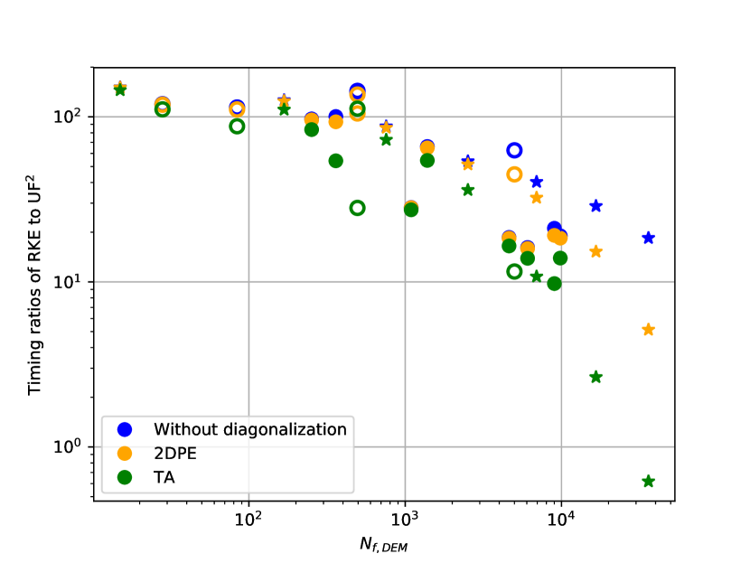
?figurename? 4: Ratio of runtimes of RKE to $\text{UF}^{2}$ for an array of vibronic systems, as described in the text. We include the diagonalization time when we calculate a single TA spectrum with 90 delay times, and a single 2DPE with 50 values of $\tau$ and 20 values of $T$. In most cases, the cost of diagonalization is negligible. Stars indicate systems with $s=k$ ranging from 2 to 8 with $S=0.02$. Open circles are systems with $s=2$ and $k$ ranging from 2 to 8, with $S$ ranging from 0.02 to 0.08. Filled circles are systems with $s=3$ and $k=3$ or $k=6$, with $S$ ranging from 0.02 to 4.5.

III.3 Comparison to split-operator pseudospectral methods

Another large class of methods useful for numerical prediction of nonlinear spectroscopies is pseudospectral methods, which use real- or Fourier-space representations of nuclear wavepackets, rather than explicit eigenstates or a basis of vibrational quanta (Domcke and Stock, 2007; Feit, Fleck, and Steiger, 1982; Kosloff and Kosloff, 1983). The widely used split-operator pseudospectral method (SOP) uses a plane-wave basis and an associated evenly-spaced real-space basis, with the efficient FFT to move between them. Briefly, SOP performs part of the time evolution due to $\hat{H}_{0}$ in position space and part in momentum space, with FFT operations between. The perturbative interaction with the pulses is also handled numerically, using a Euler method similar to that in Appendix B.1. The time step $dt$ must be short enough to resolve both the system and perturbative dynamics. It is not trivial to compare $\text{UF}^{2}$ directly to SOP methods, as the convergence parameters (e.g., $N_{c}$ for $\text{UF}^{2}$ and the grid-spacing in SOP) are not directly comparable. We compare $\text{UF}^{2}$ to the SOP implementation detailed in Ref. Yuen-Zhou et al., 2014.

For problems where a small number of eigenstates are required to describe the system dynamics, the eigenbasis used by $\text{UF}^{2}$ is considerably more efficient than a real/Fourier-space representation, which can still need many discretization points to resolve the wavepackets. In such problems, which include most of the class of problems described by Eq. 20, we expect $\text{UF}^{2}$ to greatly outperform SOP methods. Additionally, since $\text{UF}^{2}$ handles the evolution due to $\hat{H}_{0}$ exactly, $\text{UF}^{2}$ can evolve the wavefunctions forward in the absence of the pulses for near zero cost. In addition, the time step $dt$ used by $\text{UF}^{2}$ to evaluate the convolutions during the pulses is determined solely by the pulse shapes and need not be small enough to accurately resolve the dynamics in $\hat{H}_{0}$. For the cases shown in Section IV, which involve harmonic vibrational modes, $\text{UF}^{2}$ calculates spectra at least $10^{5}$ times faster than our comparison SOP method.

The SOP methods are superior to $\text{UF}^{2}$ and DP methods in cases where a continuum of eigenstates is required to describe the dynamics, as in bond-breaking, isomerization, or chemical reactions. In such cases, $\text{UF}^{2}$ easily becomes intractable and SOP is superior. In the large class of energy-transfer problems, where a discrete set of eigenstates captures the dynamics of the system, we believe $\text{UF}^{2}$ will generally outperform SOP methods.

IV Example

In this section we study a system that has the smallest Hilbert space considered in Fig. 4, in which wavefunctions may be represented using $N_{c}=28$ terms. This small size allows us to generate TA spectra in a matter of seconds, and therefore it is easy to run fast parameter sweeps and map out how spectroscopic observables change.

We explore nonlinear optical spectra for a model system presented by Tiwari and Jonas (Tiwari and Jonas, 2018).

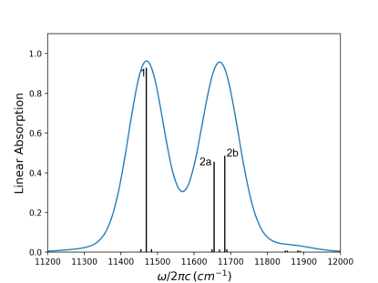
?figurename? 5: Linear absorption stick spectrum calculated using the same eigenstates as in Ref. Tiwari and Jonas, 2018. The frequencies of the stick spectra are the eigenenergies of the Hamiltonian Eq. 20 with $k=s=2$, $\omega_{i}=200\,\text{cm}^{-1}$ and $S_{i}=0.025$ for each monomer subunit. The two subunits have dipoles $|\mu_{ag}|=|\mu_{bg}|$ and $\boldsymbol{\mu}_{ag}\cdot\boldsymbol{\mu}_{bg}=0$. The heights of the sticks are $|\hat{\boldsymbol{\mu}}_{\phi^{\prime}\phi}|^{2}$. The spectrum is thermally averaged at a temperature of 80 K, using the 3 lowest energy ground vibrational states, $\Ket{00},\Ket{01},\Ket{10}$. The blue curve represents the absorption cross-section, which is obtained by broadening the stick spectrum with homogeneous and inhomogenous linewidths of $10\,\text{cm}^{-1}$ and $45\,\text{cm}^{-1}$, respectively.

Their model system is inspired by the Fenna-Matthews-Olson complex (Fenna and Matthews, 1975) and consists of a molecular dimer formed from two electronic TLS , each locally coupled to a single harmonic vibrational mode, which is the case of $k=s=2$ from Eq. 20.

The system couples to optical pulses in the electric-dipole approximation, with transition dipole matrix elements $\boldsymbol{\mu}_{ga}$ and $\boldsymbol{\mu}_{gb}$. Following Ref. 36, we consider the homodimer to have nearly identical subunits, with identical vibrational frequencies $\omega_{a}=\omega_{b}=200\,\text{cm}^{-1}$, Huang-Rhys factors $S=0.025$, and with $E_{b}-E_{a}=150$ cm^-1. We consider that $\boldsymbol{\mu}_{ga}$, $\boldsymbol{\mu}_{gb}$ have the same magnitude but extend the model by varying the angle $\theta$ between these transition dipoles, corresponding to varying the angle between the two subunits. Due to the small Huang-Rhys factors considered in Ref. Tiwari and Jonas, 2018, only a small number of vibrational states contribute to third-order spectra, allowing truncation of the vibrational Hilbert space, as described in Sec. II.5. Reference Tiwari and Jonas, 2018 did not calculate TA spectra; first we compare our results for linear absorption and then present our TA predictions.

Reference Tiwari and Jonas, 2018 demonstrates how the Huang-Rhys factors split one exciton peak into two vibronic peaks. We plot the linear absorption spectrum for this system in Fig. 5, choosing lineshape parameters to visually reproduce results from Ref. Tiwari and Jonas, 2018. We label the peaks in Fig. 5 following Tiwari and Jonas. There are two broad peaks centered around $f_{1}=11469.5\,\text{cm}^{-1}$ and $f_{2}=11669.6\,\text{cm}^{-1}$, with the latter composed of two peaks, $2a$ and $2b$, separated by $\Omega_{1}=29\,\text{cm}{}^{-1}$. However, this splitting is invisible to linear absorption because peaks $2a$ and $2b$ smear together.

$\Omega_{1}$ is, however, the dominant beat frequency in a TA experiment, shown in Fig. 6, corresponding to oscillations repeating about every 1.15 ps. The TA signal is detected as two broad features centered at $f_{1}$ and $f_{2}$. Notably, the oscillations centered around $f_{1}$ are roughly $90^{\text{o}}$ out of phase with those at $f_{2}$, and there is a node halfway between them. This type of nodal feature is widely observed and has been studied in many vibrational systems (Liebel et al., 2015; McClure et al., 2014; Cina et al., 2016).

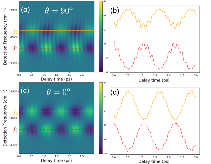
?figurename? 6: Transient absorption with Gaussian pump and probe pulses centered on $f_{2}$ and with FWHM of 12 fs. (a) Dipole angle $\theta=90^{\text{o}}$, (b) linecuts of (a) at $f_{2}$ (orange) and $f_{1}$ (red, dash-dotted), (c) Dipole angle of $\theta=0^{\text{o}}$, (d) linecuts of (c) at $f_{2}$ (orange) and $f_{1}$ (red, dash-dotted). In both cases the low-frequency beats are out of phase between $f_{1}$ and $f_{2}$. The high-frequency beats are in phase between $f_{1}$ and $f_{2}$ for $\theta=90^{\text{o}}$ and are reduced in amplitude and out of phase for $\theta=0^{\text{o}}$.

As mentioned in Section II.E, to achieve convergence of these TA spectra to within 1%, it is sufficient to have $N_{f,DEM}=N_{f,GSM}=15$ and $N_{f,SEM}=30$, while $N_{c,DEM}=N_{c,GSM}=10$ and $N_{c,SEM}=8$. Each TA spectrum is isotropically averaged, with the same homogeneous and inhomogeneous linewidths in the linear absorption spectrum. Each TA spectrum, which is of the form $S_{TA}(T,\omega)$, consists of $m_{T}=180$ delay times, and $M_{t}=286$, 562, 1391 detection frequency points for FWHM pulse durations of 62, 31 and 12 fs, respectively, and takes about 3 seconds to generate on a 2.3GHz Macbook Pro. The equivalent calculation using the SOP code (see Section III.3) would take almost 6 days to converge to the same accuracy if run on the same machine. This system is the leftmost point of Fig. 4, and the RKE method would take over 7 minutes to produce each spectrum.

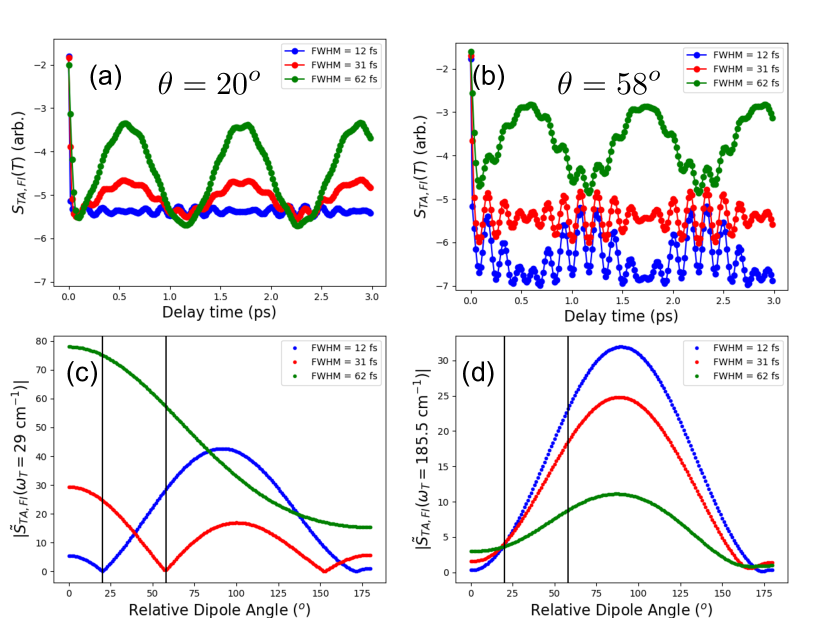
?figurename? 7: Demonstration of parameter variations for the same system as in Fig. 6. Panels (a) and (b) show frequency-integrated transient absorption (FITA) spectra for (a) $\theta=20^{\text{o}}$ and (b) $\theta=58^{\text{o}}$ with three different Gaussian pulse durations. There are two prominent time scales present: the $\Omega_{1}$ beat (corresponding to the 1.15 ps oscillation) and the $\Omega_{2}$ and $\Omega_{3}$ beats (corresponding to the 180 fs and 156 fs oscillations). Panels (c) and (d) show the magnitude of these beats of the FITA spectra at (c) $\omega_{T}=\Omega_{1}$ and (d) $\omega_{T}=\Omega_{2}$ as a function of $\theta$. Black vertical lines indicate $\theta$ from panels (a) and (b). Note that at $\omega_{T}=\Omega_{1}$, the FITA magnitude shows a dramatic dependence on both dipole angle and electric field shape, demonstrating the importance of taking into account electric field shapes. The signals at $\omega_{T}=\Omega_{2}$ are less sensitive.

The efficiency of $\text{UF}^{2}$ enables rapid study of a wide range of parameters. The frequency-integrated TA signal,

$$S_{FI,TA}(T)=\int\mathrm{d}\omega S_{TA}(T,\omega),$$ (24)

is particularly sensitive to electric field shape (Yuen-Zhou, Krich, and Aspuru-Guzik, 2012; Johnson et al., 2014). Figure 7(a,b) shows frequency-integrated TA spectra with dipole angles $\theta=20^{\circ}$, $58^{\circ}$ and three optical pulse durations. The responses with different pulse shapes are quite different for both values of $\theta$. In order to study the differences over a wide range of $\theta$ we study the Fourier transform of $S_{FI,TA}(T)$ with respect to the delay time:

$$\tilde{S}_{FI,TA}(\omega_{T})=\frac{1}{\sqrt{2\pi}}\int_{-\infty}^{\infty}\mathrm{d}TS_{FI,TA}(T)e^{i\omega_{T}T},$$

and track the response at $\omega_{T}=\Omega_{1}$ and $\omega_{T}=\Omega_{2}=f_{2a}-f_{1}=185.5\,\text{cm}^{-1}$ in Fig. 7(c,d). A nearly impulsive pulse (12 fs FWHM - blue curves) gives a dramatically different response as compared to somewhat longer pulses (35 fs - red curves, 70 fs - green curves). Notice that the longest pulse considered here is still short compared to the fastest time scale of the system, $\Omega_{3}$, corresponding to a period of 156 fs, so the large changes of the signals with pulse duration are a warning sign that accurate study of finite-pulse effects is important to correctly model nonlinear spectra. This study is easily tractable using $\text{UF}^{2}$, taking only 30 minutes to run, but would have taken 3 days to run using RKE and more than a year using our SOP implementation on the same computer.

V Conclusion

$\text{UF}^{2}$ is a computationally efficient method for calculating perturbative nonlinear spectroscopies of systems with finite dimensional relevant Hilbert spaces. It includes all finite-duration and pulse-overlap effects, enabling accurate modeling of and fitting to nonlinear spectroscopic data. The current introduction has focused on closed systems, but $\text{UF}^{2}$ can be readily extended to open systems with time-independent Liouvillians, in which case its cost scales as $N_{c}^{4}$ rather than $N_{c}^{2}$, where $N_{c}$ is the relevant Hilbert space dimension. We have shown the methods that can be used to aggressively reduce the required dimension $N_{c}$, which enables $\text{UF}^{2}$ to be highly efficient for small systems and competitive for surprisingly large problems. For vibronic systems with thousands of relevant states, $\text{UF}^{2}$ generally outperforms our comparison DP method and is competitive for many systems with tens of thousands of relevant states; for larger systems, DP methods are generally superior.

The intent of the publicly available $\text{UF}^{2}$ code is to present a package that makes it easy to translate Feynman diagrams into code. Since $\text{UF}^{2}$ readily enables consideration of arbitrary pulse shapes, the effects of pulse durations, chirps, etc. on nonlinear spectroscopies can now be included as a matter of course in analyses of experiments. Given the large number of problems under active study with tens to hundreds of relevant states, we hope that $\text{UF}^{2}$ will enable easy and rapid spectroscopic prediction and analysis including pulse shape effects that are often neglected.

?appendixname? A Computational cost of $\text{UF}^{2}$

We derive the computational cost of $\text{UF}^{2}$, highlighting which parameters are required for convergence and which are at the user’s discretion, focusing on the case of a 2DPE rephasing spectrum, as in Eq. 8.

We derive the computational cost of calculating the 2DPE rephasing signal. We briefly outline what is required for this calculation by working backwards from Eq. 8. Symbols used in this section are summarized in Table 3. Calculation of the signal requires that we determine $\boldsymbol{P}_{\text{2D}}^{(3)}(\tau,T;\omega)$ at the desired values of $\tau$ and $T$. $\text{UF}^{2}$ directly calculates $\boldsymbol{P}_{\text{2D}}^{(3)}(t)$ for one pair of $(\tau,T)$ at a time. We calculate $\boldsymbol{P}_{\text{2D}}^{(3)}(t)$ at sufficient time points, $M_{t}$, in order to obtain the desired frequency resolution. The cost of the FFT to obtain $\boldsymbol{P}_{\text{2D}}^{(3)}(\omega)$ from $\boldsymbol{P}_{\text{2D}}^{(3)}(t)$ is negligible compared with the other costs of $\text{UF}^{2}$. Assuming that we require the polarization field at $m_{\tau}$ values of $\tau$ and $m_{T}$ values of $T$, the cost of the full spectrum is $m_{\tau}m_{T}\text{Cost}(\boldsymbol{P}_{\text{2D}}^{(3)}(t))$. $\boldsymbol{P}_{\text{2D}}^{(3)}(t)$ is a sum of three Feynman diagrams (see Fig. 1), each of which is calculated separately. We focus on $\boldsymbol{P}_{ESA}^{(3)}(t)$, which is often the dominant cost. The cost of the other diagrams follows directly from this derivation.

?tablename? 3: Summary of symbols used to describe computational cost of a 2DPE rephasing signal. $M$, $M_{E}$, $\epsilon$, and $dt$ are convergence parameters.

Symbol	Definition
$M$	Number of time points to resolve pulses $\text{UF}^{2}$
$M_{E}$	Number of time points to resolve pulse in RKE
$\epsilon$	Local tolerance of RK45 algorithm
$dt$	Fixed step size for RKE and $\text{UF}^{2}$ during pulses
$dt_{RK}$	Adaptive step size of RK45 algorithm

Using Eq. 17, the cost of $\boldsymbol{P}_{ESA}^{(3)}(t)$ can be broken into three parts: calculating the two necessary perturbed wavepackets and the cost of the dipole matrix element of those wavepackets. This latter cost turns out to be the dominant cost asymptotically. Since $\Ket{\psi_{a}(t)}=K_{a}\Ket{\psi^{(0)}(t)}$ and $\Ket{\psi_{bc}(t)}=K_{c}K_{b}\Ket{\psi^{(0)}(t)}$, the cost of calculating these wavepackets is, at first glance, the cost of three calls to the $K_{j^{(*)}}$ operator, which is the heart of $\text{UF}^{2}$. However, $\Ket{\psi_{a}(t)}$ corresponds to the interaction with the first pulse, which arrives at a fixed time, and therefore need only be calculated once. Further, $\Ket{\psi_{b}(t)}$ corresponds to the second pulse, which arrives at $m_{\tau}$ different coherence times $\tau$. Therefore $\Ket{\psi_{b}(t)}$ only needs to be calculated $m_{\tau}$ different times. The only wavefunction that must be recalculated for every pair $\tau,T$ is the one caused by the third interaction, $\Ket{\psi_{bc}(t)}$. Therefore the dominant cost of calculating the perturbative wavefunctions for many different values of $T$ is simply one call to $K_{c}$.

To determine the cost of $K_{j^{(*)}}$, we first explain how wavefunctions are stored in $\text{UF}^{2}$. Each wavefunction is represented in the same way. For example, the second-order wavefunction is

$$\Ket{\psi_{bc}(t)}=\sum_{\phi=1}^{N_{c,DEM}}e^{-i\omega_{\phi}t}c_{\phi,ac^{*}}(t)\Ket{\phi},$$ (25)

where each of the $c_{\phi,ac^{*}}(t)$ are calculated at $M$ evenly spaced time points . The spacing $dt$ is determined by the shape of the pulse amplitude $A_{i}(t)$ (see Eq. 4). Recall from Eq. 16 that $c_{\phi,pj^{(*)}}(t)$ only varies in the interval $(t_{j,\min},t_{j,\max})$. Outside of this interval, $c_{\phi,pj^{(*)}}$ is constant and can thus be trivially extended to any time points needed. This property allows wavefunctions to be stored for re-use without a significant memory cost. For simplicity in this discussion we assume that $t_{j,\max}-t_{j,\min}$ is the same for each pulse. Since we are discretizing a continuous convolution integral, $M=\frac{t_{j,\max}-t_{j,\min}}{dt}$ is a convergence parameter. For any electric field that does not go strictly to zero, the choice of $t_{j,\min}$ and $t_{j,\max}$ must also be checked for convergence.

Inspecting Eq. 14, the cost of $\hat{K}_{j}$ is $N_{c,X}$ times the cost of evaluating $\theta*y_{\phi}$ to obtain $c_{\phi,pj}$. Calculating $y_{\phi}$ is dominated by the cost of taking the dipole-weighted sum over $\phi^{\prime}$ (we are neglecting the small cost of multiplying by the pulse amplitude $\varepsilon_{j}^{(*)}$ and by the time evolution factors $e^{i\omega_{\phi}(t-t^{\prime})}$ and $e^{-i\omega_{\phi^{\prime}}(t-t^{\prime})}$). The sum has a cost of $\alpha N_{c,X}M$, where $\alpha$ is the cost of multiplying two complex numbers. We calculate $\theta*y_{\phi}$ using the convolution theorem and the FFT. Since we are interested in the linear convolution, we evaluate $\theta$ at $2M-1$ points and zero-pad $y_{\phi}$ to be size $2M-1$. We only calculate the FFT of $\theta$ once, making that cost negligible. We calculate the FFT of $y_{\phi}$, which has a cost of $\beta^{\prime}(2M-1)\log_{2}\left(2M-1\right)\approx 2\beta^{\prime}M\log_{2}M+O(M)$, where $\beta^{\prime}$ depends upon the implementation of the FFT. We multiply the two ($\tilde{y}_{\phi}$ and $\tilde{\theta}$), which has cost $O(M)$, and then take the inverse FFT of the product (cost $2\beta^{\prime}M\log_{2}M+O(M)$). Thus the total cost of the convolution is $4\beta^{\prime}M\log_{2}M+O(M)$. The cost to obtain one coefficient $c_{\phi,pj^{(*)}}(t)$ to highest order in $M$ and $N$ is then

$$\text{Cost}(c_{\phi,pj^{(*)}}(t))=\alpha N_{c,X}M+\beta M\log_{2}M+O(M),$$ (26)

where $\beta=4\beta^{\prime}$. The cost of calling $K_{j^{(*)}}$ is then $N_{c,Y}\text{Cost}(c_{\phi,pj^{(*)}})$, where $N_{c,X}$ is the dimension of the old manifold and $N_{c,Y}$ is the dimension of the new manifold, giving

$$\text{Cost}(K_{j^{(*)}})=N_{c,Y}M(\alpha N_{c,X}+\beta\log_{2}M)+O(MN_{c,Y}),$$ (27)

and so $\text{Cost}(K_{j^{(*)}})\sim MN_{c,X}N_{c,Y}$ for large $N_{c}$. In the case of $\Ket{\psi_{bc}(t)}$, then, we have a cost $\sim MN_{c,SEM}N_{c,DEM}$. Given that $N_{c,DEM}$ is often the largest value of $N_{c,X},X\in\{GSM,SEM,DEM\}$, the ESA diagram often dominates the cost of $\text{UF}^{2}$. The other diagrams involve wavefunctions that move between the GSM and the SEM, and therefore the cost of each $K_{j}$ scales as $N_{c,GSM}N_{c,SEM}$.

Once we know each of the necessary wavefunctions at its $M$ time points, we evolve the wavefunctions using $\hat{U}_{0}$ to include $M_{t}$ times points, in order to obtain the desired frequency resolution of the final spectrum. The $M_{t}$ points are spaced by the same $dt$, and span from just before the last pulse arrives, $t_{c,\min}$, until the signal has decayed to an appropriate cut-off due to the optical dephasing described in Section II.3. This evolution is of negligible cost since we know the exact form of $\hat{U}_{0}(t)$.

We then calculate the expectation value $\boldsymbol{P}_{ESA}^{(3)}(t)=\Bra{\psi_{a}(t)}\hat{\boldsymbol{\mu}}\Ket{\psi_{bc}(t)}$, which has a cost of $\alpha N_{c,SEM}N_{c,DEM}(M+M_{t})$, since the polarization field must capture both the pulse turn-on described by $M$ points, and the decay of the field described by the additional $M_{t}$ points, so in total $\text{Cost}(\boldsymbol{P}_{ESA}^{(3)}(t))=\alpha N_{c,SEM}N_{c,DEM}(M+M_{t})+\text{Cost}(K_{j})$. The signal must be calculated at $m_{\tau}$ $\tau$ points and $m_{T}$ $T$ points, so we arrive at the full cost of the ESA signal

$$\text{Cost}(S_{ESA}(\tau,T,\omega)) =m_{\tau}m_{T}\bigg{(}\alpha N_{c,SEM}N_{c,DEM}(M+M_{t})$$

$$+N_{c,DEM}M\big{(}\alpha N_{c,SEM}+\beta\log_{2}M\big{)}\bigg{)}$$ (28)

to highest order in $N_{c,X}$, $M_{t}$ and $M$. In general we find that $M<M_{t}$, and the cost of evaluating the necessary wavefunctions is sometimes less than half of the cost of obtaining the total signal. In Section IV, we calculate the TA signal, which is composed of four Feyman diagrams with costs less than or equal to that in Eq. 28, with $m_{\tau}=1$, since the TA signal has $\tau=0$. In Section IV we use $M=21$ and $M_{t}\approx 1000$, in order to achieve convergence of better than $1\%$.

Assuming that $M<M_{t}$, and that $\alpha N_{c}\gg\beta\log_{2}M$, the total cost scales as

$$C_{\text{UF}^{2}}(S_{ESA})\sim m_{\tau}m_{T}N_{c,SEM}N_{c,DEM}M_{t}.$$ (29)

Note that $\text{UF}^{2}$ assumes that the eigenvalues and eigenstates of $\hat{H}_{0}$ have already been attained. If the dimension of $\hat{H}_{0}$ is $N_{f}$, then the computational cost of that diagonalization can scale as $N_{f}^{3}$, which can exceed the cost of $\text{UF}^{2}$ itself, especially since $\text{UF}^{2}$ reduces the relevant Hilbert space dimension $N_{c}$ so aggressively. For many systems, however, $\hat{H_{0}}$ is sparse, allowing efficient iterative methods to be used to find its eigenvalues and eigenstates. The scaling of those algorithms is beyond the scope of this manuscript, but we simply note that there are many important cases where solving $\hat{H}_{0}$ is not computationally limiting. For example, vibronic systems of coupled chromophores, each with local harmonic oscillators, are extremely sparse, and an efficient algorithm to determine their eigenstates will be detailed separately.

?appendixname? B RKE implementation and scaling

B.1 Implementation

Direct propagation (DP) methods solve the Schrodinger equation

$$\frac{d\Ket{\psi^{(n)}(t)}}{dt}=-iH_{0}\Ket{\psi^{(n)}(t)}-iH^{\prime}_{j}(t)\Ket{\psi^{(n-1)}(t)},$$

where we have set $\hbar=1$, by propagating the ODE forward in time domain.

In order to compare the cost of $\text{UF}^{2}$ to the cost of DP methods, we have implemented a hybrid DP method that uses the adaptive-step size 4-5${}^{\text{th}}$ order Runge-Kutta ODE solver from scipy (called RK45) to propagate the system dynamics

$$\frac{d\Ket{\psi^{(n)}}}{dt}=-iH_{0}\Ket{\psi^{(n)}},$$

and uses the first-order Euler method to include the perturbation

$$-iH^{\prime}_{j}(t)\Ket{\psi^{(n-1)}(t)},$$

with a previously calculated lower-order wavepacket $\Ket{\psi^{(n-1)}(t)}$, as described in Refs. Engel, 1991; Yuen-Zhou et al., 2014. As with $\text{UF}^{2}$, we assume that each pulse $\boldsymbol{E}_{j}$ is non-zero only during times $t_{j,\text{min}}<t<t_{j,\text{max}}$. When all of the pulses are zero, propagation is simply handled by RK45. Given a local absolute and relative tolerance $\epsilon$, RK45 can integrate from $t_{i}$ to $t_{f}$ using an adaptively determined step size $dt_{RK}$. The wavefunctions are stored at equally spaced time points with time step $dt$, which must be short compared to the optical pulses and in our implementation we set to the same $dt$ used in $\text{UF}^{2}$. This fixed time step is used for the Euler method and allows the reuse of lower-order wavefunctions for many values of pulse delay times. Note that as mentioned at the end of Section III.2, this choice of $dt$ does not converge the RKE spectra to the same accuracy as $\text{UF}^{2}$. Given a state vector $\Ket{\psi(t_{i})}$, we use the notation $\Ket{\psi(t_{i}+dt)}=U_{0}(dt)\Ket{\psi(t_{i})}$ to represent the RK45 propagation.

To include the perturbation $H^{\prime}_{j}(t)$, we begin by defining the first-order wavefunction $\Ket{\psi_{a}(t<t_{a,\text{min}})}=0$. We define $\Ket{\psi_{a}(t_{a,\text{min}})}=-iH_{a}^{\prime}(t_{a,\text{min}})dt\Ket{\psi^{(0)}(t_{a,\text{min}})}$, where $\Ket{\psi^{(0)}(t_{a,\text{min}})}$ is a stationary state (possibly with an evolving phase factor). We propagate until $t_{a,\text{max}}$ in steps of size $dt=(t_{a,\text{max}}-t_{a,\text{min}})/M_{E}$. Let $m$ run from 0 to $M_{E}$. Then

$$\Ket{\psi_{a}(t_{a,\text{min}}+mdt)}=U_{0}(dt)\Ket{\psi_{a}(t_{a,\text{min}}+(m-1)dt)}\\ +i\boldsymbol{\mu}\cdot\boldsymbol{e}_{a}\varepsilon_{a}(t_{a,\text{min}}+mdt)\Ket{\psi^{(0)}(t_{a,\text{min}}+mdt)}.$$

Once we have obtained $\Ket{\psi_{a}(t_{a,\text{max}})}$, we obtain $\Ket{\psi_{a}(t>t_{a,\text{max}})},$ using RK45 alone. This method works in general for the $n^{th}$ order wavefunction generated by an interaction with the $j^{th}$ pulse. Given the $\left(n-1\right)^{\text{st}}$ wavefunction $\Ket{\psi_{p}(t)}$, we define $\Ket{\psi_{pj^{(*)}}(t_{j,\text{min}})}=i\boldsymbol{\mu}\cdot\boldsymbol{e}_{j}^{(*)}\varepsilon_{j}^{(*)}(t_{j,\text{min}})\Ket{\psi_{p}(t_{j,\text{min}})}$, and then at all times until $t_{j,\text{max}}$ using

$$\Ket{\psi_{pj^{(*)}}(t_{a,\text{min}}+mdt)}=U_{0}(dt)\Ket{\psi_{pj^{(*)}}(t_{a,\text{min}}+(m-1)dt)}\\ +i\boldsymbol{\mu}\cdot\boldsymbol{e}_{j}^{(*)}\varepsilon_{j}^{(*)}(t_{a,\text{min}}+mdt)\Ket{\psi_{p}(t_{a,\text{min}}+mdt)}.$$

Once again, for all times after $t_{j,\text{max}}$, we only use RK45 to propagate the wavefunction in its manifold.

B.2 Computational cost analysis

We derive the computational cost of calculating the 2DPE rephasing signal, now using the RK45-Euler hybrid (RKE) method outlined in Section B.1, following a similar path as our derivation of the cost of $\text{UF}^{2}$, working backwards from Eq. 8. Symbols used in this section are summarized in Tables 1-3. As for $\text{UF}^{2}$, we begin by considering the ESA diagram, and derive the cost of $\boldsymbol{P}_{ESA}^{(3)}(t)$.

The cost of RKE is the cost of obtaining the necessary wavefunctions, $\Ket{\psi_{a}(t)}$ and $\Ket{\psi_{bc}(t)}$, and computing $\boldsymbol{P}_{ESA}(t)=\Bra{\psi_{a}(t)}\boldsymbol{\mu}\Ket{\psi_{bc}(t)}$. In the Condon approximation, $\boldsymbol{\mu}$ is a sparse rectangular matrix consisting of diagonal blocks, so this expectation value has a cost of $\alpha qr_{\mu}N_{f,DEM}$. Even outside of the Condon approximation, $\boldsymbol{\mu}$ is still sparse, and therefore the cost is still $O(N_{f})$; the number of entries per row, $r_{\mu}$, is simply a little larger.

The remaining cost is the cost of obtaining the necessary wavefunctions. The cost of obtaining a perturbative wavefunction breaks down into two parts: the cost of the RK45 algorithm to propagate $H_{0}$ and the cost of the Euler method to include the perturbation $H_{j}^{\prime}$. We first derive the cost of RK45 for times after $t>t_{j,\text{max}}$, where RK45 can take full advantage of its adaptive step size. In this regime, the user sets a local tolerance $\epsilon$, and RK45 determines what step size $dt_{RK}$ satisfies that tolerance, and we approximate it as a constant. To take each step, RK45 must make 6 function evaluations of the form $H_{0}\Ket{\psi}$ and sum the results with the required weights. Each evaluation has the cost of a sparse matrix-vector multiplication, $\alpha qrN_{n,X}$, where $r$ is the average number of non-zero entries of $H_{0}$ per row and $q$ is an additional overhead factor for sparse matrix operations. Ignoring the extra costs when steps are rejected, we thus find that the cost to take a step $dt_{RK}$ is $6\alpha(qr+1)N_{f}\approx 6\alpha qrN_{f,X}$. Assuming we need to know the wavefunction at some final time $t_{f}>t_{j,\text{max}}$, the cost of propagating the wavefunction when the pulse is off,

$$C_{RK} =6\alpha qrN_{f,X}M_{RK},$$

where $M_{RK}=(t_{f}-t_{j,\text{max}})/dt_{RK}$ is the required number of steps after the pulse ends. This wavefunction can be relatively inexpensively evaluated on a mesh with spacing $dt$ using the RK45 interpolator, but the computational cost is set by the adaptively optimized $dt_{RK}$.

During the time when the pulse is non-zero, the cost of the RK45 portion of the evolution is

$$6\alpha qrN_{n,X}\max\left(M_{E},(t_{j,\text{max}}-t_{j,\text{min}})/dt_{RK}\right),$$

where $M_{E}=(t_{j,max}-t_{j,min})/dt$. If $dt$ is smaller than $dt_{RK}$, we must pay an additional cost of taking smaller steps than field-free evolution using RK45 would require. We must also pay the cost of adding in the perturbation. Again, since $\boldsymbol{\mu}$ is a sparse matrix with $r_{\mu}$ entries per row, the cost of $\boldsymbol{\mu}\Ket{\psi}$ is $\alpha qr_{\mu}N_{f}$. The cost of evaluating $\varepsilon_{j}$ at a single time point is negligible, and so the cost of adding in the perturbation is $\alpha qr_{\mu}N_{n,X}M_{E}.$ Assuming that $dt<dt_{RK}$, we can easily add these costs to obtain the cost of propagating when the pulse is on,

$$C_{E} =\alpha q(6r+r_{\mu})N_{n,X}M_{E}.$$

Thus the cost of calculating a single wavefunction is

$$C_{RKE}\left(\Ket{\psi_{pj^{(*)}}}\right) =C_{E}+C_{RK}$$

Despite the fact that $dt$ is generally smaller than $dt_{RK}$, it is still often the case that $M_{RK}>M_{E}$. In general we find that $M_{E}=100$ is usually sufficient to resolve the pulse interaction and converge the spectroscopic signals to within 1%. In contrast, we often find that $M_{RK}>100$, and therefore the cost of obtaining a perturbative wavefunction is usually dominated by the propagation cost in the absence of the electric field. This observation depends upon the imposed decay of the polarization field, $\gamma$, as described in Section II.3. As for $\text{UF}^{2}$, once the polarization field is obtained, we multiply by $e^{-\gamma|t-t_{probe}|}$, and therefore we generally need to resolve the wavefunction to $t_{f}=t_{\text{probe}}+\frac{5}{\gamma}$.

We developed this hybrid method for the purposes of making a fair comparison with $\text{UF}^{2}$. We assert that if $C_{E}>C_{RK}$, there is likely a more efficient algorithm, for example using RK45 both while the pulse is on and when the pulse is off. For the purposes of comparison, we make sure to operate in a regime where $C_{E}<C_{RK}$, and therefore we approximate $C_{RKE}\approx C_{RK}$.

This process must be repeated 3 times in order to calculate the ESA at a single pair of pulse delays $\tau,T$. However, $\Ket{\psi_{a}}$ only needs to be calculated once, and can be stored and re-used because we are working with a regularly spaced time grid. Similarly, $\Ket{\psi_{b}}$ only needs to be calculated once for each value of $\tau$ but can be reused for all values of $T$. The only wavefunction that must be recalculated each time is $\Ket{\psi_{bc}}$, and therefore this cost dominates the cost of obtaining $\boldsymbol{P}_{ESA}$. Therefore

$$C_{RKE}(S_{ESA}) \approx m_{\tau}m_{T}C_{RK}$$ (30)

Note that the costs of the other diagrams contributing to $\boldsymbol{P}^{(3)}(t)$ have a similar form, but scale as $N_{f,SEM}$ or $N_{f,GSM}$. Since $N_{f,SEM},N_{f,GSM}<N_{f,DEM}$ in general, the cost of obtaining the rephasing signal is dominated by the cost of $\boldsymbol{P}_{ESA}$.