UCHEP–19–01
Semileptonic and leptonic charm meson decays at Belle II

Abstract

We review measurements of semileptonic and leptonic charm meson decays performed by the Belle experiment, and we use these results to estimate the sensitivity of the follow-on Belle II experiment to these decays.

1 Introduction

Semileptonic and leptonic $D$ meson decays are easier to understand theoretically than hadronic decays, as the hadronic uncertainties factorize. They are also straightforward to measure at an $e^{+}e^{-}$ experiment due to low backgrounds and good detector hermeticity. They have been studied at experiments CLEOc [1], BESIII [2], Belle [3], and Babar [4], and they constitute an important part of the physics program of Belle II [5]. The Belle II experiment runs at the SuperKEKB accelerator at the KEK laboratory in Japan and is the follow-on experiment to Belle. The accelerator collides 4 GeV/$c$ positrons with 7 GeV/$c$ electrons; the center-of-mass energy is tuned to be at the $\Upsilon(4S)$ resonance in order to produce copious amounts of $B$ mesons via $e^{+}e^{-}\!\rightarrow\!\Upsilon(4S)\!\rightarrow\!B\bar{B}$. The Belle II detector is now being commissioned and will begin taking physics data in the spring of 2019. In this paper we review measurements of leptonic and semileptonic charm decays made by the preceding Belle experiment, and we use these results to estimate the expected sensitivity of Belle II.

2 Leptonic decays

The partial width $\Gamma(D^{+}_{(s)}\rightarrow\ell^{+}\nu)$ [6] is given by the formula [7]

$$\Gamma(D^{+}_{(s)}\!\rightarrow\!\ell^{+}\nu) = \frac{G^{2}_{F}}{8\pi}f^{2}_{D_{(s)}}|V_{cx}|^{2}m_{D_{(s)}}\,m^{2}_{\ell}\left(1-\frac{m^{2}_{\ell}}{\ \ m^{2}_{D_{(s)}}}\right)^{2},$$ (1)

where $f_{D_{(s)}}$ is the $D^{+}_{(s)}$ decay constant, and $V_{cx}$ is the Cabibbo-Kobayashi-Maskawa (CKM) matrix element $V_{cs}$ for $D^{+}_{s}$ decays and $V_{cd}$ for $D^{+}$ decays [8]. The decay constant $f_{D_{(s)}}$ parameterizes the hadronic matrix element $\langle 0|{\cal H}|D^{+}_{(s)}\rangle$. To test the Standard Model (SM), one measures the branching fraction $B(D^{+}_{(s)}\rightarrow\ell^{+}\nu)$, calculates the partial width $\Gamma=B/\tau_{D}$, and uses Eq. (1) to determine the product $f_{D_{(s)}}|V_{cx}|$. One then either takes $|V_{cx}|$ from other measurements and CKM unitarity to extract $f_{D_{(s)}}$, or takes $f_{D_{(s)}}$ from lattice QCD theory to extract $|V_{cx}|$.

The Heavy Flavor Averaging Group (HFLAV) [9] has calculated world average (WA) values of the product $f_{D_{(s)}}|V_{cx}|$ using all relevant experimental measurements; the results are shown in Fig. 1.

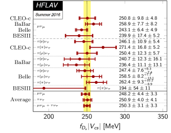
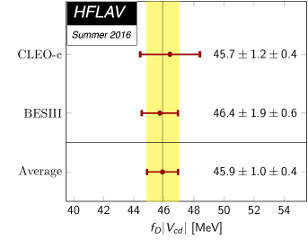
Figure 1: World average (WA) values as calculated by the Heavy Flavor Averaging Group (HFLAV) [9] for the products $f_{D_{s}}|V_{cs}|$ (left) and $f_{D}|V_{cd}|$ (right).

The WA values are $f_{D_{s}}|V_{cs}|=(250.3\pm 3.1\pm 3.3)$ MeV and $f_{D}|V_{cd}|=(45.9\pm 1.0\pm 0.4)$ MeV. The Flavor Lattice Averaging Group [10] quotes $f_{D_{s}}=(248.83\pm 1.27)$ MeV and $f_{D}=(212.15\pm 1.45)$ MeV based on lattice QCD results from Refs. [11, 12]. Inserting these values gives

$$|V_{cs}| = 1.006\pm 0.018\pm 0.005$$ (2)

$$|V_{cd}| = 0.2164\pm 0.0050\pm 0.0015\,,$$ (3)

where the first error is experimental and the second is from theory. Alternatively, inserting more recent (and precise) lattice QCD results $f_{D_{s}}=(249.9\pm 0.4)$ MeV and $f_{D}=(212.7\pm 0.6)$ MeV from the Fermilab/MILC Collaboration [13] gives essentially identical results for $|V_{cs}|$ and $|V_{cd}|$.

Conversely, inserting CKM matrix elements $|V_{cs}|=0.973394\,^{+0.000074}_{-0.000096}$ and $|V_{cd}|=0.22529\,^{+0.00041}_{-0.00032}$ as obtained by the CKM Fitter group [14] from a global fit to various measurements subject to CKM unitarity [8], we obtain

$$f_{D_{s}} = (257.1\pm 4.6)~{}{\rm MeV}$$ (4)

$$f_{D} = (203.7\pm 4.9)~{}{\rm MeV}\,.$$ (5)

These values are consistent with those calculated from lattice QCD.

——————

Belle has measured $D^{*+}_{s}\!\rightarrow\!D^{+}_{s}\gamma$, $D^{+}_{s}\!\rightarrow\!\mu^{+}\nu$ decays using 913 fb^-1 of data [15]. The analysis proceeds in four steps:

1. a $D^{(*)0}$, $D^{(*)+}$, or $\Lambda^{+}_{c}$ decay is reconstructed on the “tag-side” of an event, i.e., recoiling against the signal-side $D^{+}_{s}\!\rightarrow\!\mu^{+}\nu$ decay. To conserve strangeness, a $K^{\pm}$ or $K^{0}_{S}$ is also required on the tag side. If a $\Lambda^{+}_{c}$ decay were reconstructed, then a $\bar{p}$ is required to conserve baryon number.

2. a “fragmentation system” ($X_{\rm frag}$) is constructed from 1-3 $\pi^{\pm}$ tracks and 0-1 $\pi^{0}$ candidates. From the measured four-momenta $P$, a “missing mass” $\sqrt{P^{2}_{\rm miss}}=\sqrt{(P_{e^{+}}+P_{e^{-}}-P_{\rm tag}-P_{K}-P_{X_{\rm frag}})^{2}}$ is calculated and required to be within $3\sigma$ in resolution of $M(D^{*+}_{s})$.

3. a low-momentum $\gamma$ is required, presumably originating from $D_{s}^{*+}\!\rightarrow\!D^{+}_{s}\gamma$, and the missing mass $\sqrt{(P_{e^{+}}+P_{e^{-}}-P_{\rm tag}-P_{K}-P_{X_{\rm frag}}-P_{\gamma})^{2}}$ is calculated. This distribution should peak near $M(D^{+}_{s})$ for signal decays, and it is fitted to obtain an inclusive $D^{+}_{s}$ signal yield.

4. a high mometum $\mu^{+}$ pointing to the interaction point is required, and the missing mass $\sqrt{(P_{e^{+}}+P_{e^{-}}-P_{\rm tag}-P_{K}-P_{X_{\rm frag}}-P_{\gamma}-P_{\mu})^{2}}$ is calculated. This distribution should peak at $m_{\nu}\approx 0$ for signal decays; it is fitted to obtain the exclusive $D^{+}_{s}\!\rightarrow\!\mu^{+}\nu$ signal yield.

The results of the third step are shown in Figs. 2a,b for the two simplest $X_{\rm frag}$ systems. Fitting these distributions (and also those of the other $X_{\rm frag}$ systems) yields $94360\pm 1310\,{\rm(stat.)}\pm 1450\,{\rm(syst.)}$ inclusive $D^{+}_{s}$ decays. The result of the last step is shown in Fig. 2c; fitting this distribution yields $492\pm 26$ $D^{+}_{s}\!\rightarrow\!\mu^{+}\nu$ decays.

This method can also be used at Belle II. As the Belle measurement is limited by statistics rather than systematics, we scale the event yields obtained by Belle by the ratio of luminosities. The result is $5.2\times 10^{6}$ inclusive $D^{+}_{s}$ decays, and 26900 exclusive $D^{+}_{s}\!\rightarrow\!\mu^{+}\nu$ decays, in 50 ab^-1 of Belle II data. The latter sample should yield statistical errors of $\delta|V_{cs}|=0.003$ and $\delta f_{D_{s}}=0.8$ MeV, which are similar to the current theoretical errors arising from lattice QCD.

A similar analysis was performed at Belle for $D^{+}_{s}\!\rightarrow\!\tau^{+}\nu$ decays [15]. In this case a yield of $2217\pm 83$ exclusive decays were obtained. Scaling this yield by the ratio of Belle and Belle II luminosities yields 121400 $D^{+}_{s}\!\rightarrow\!\tau^{+}\nu$ decays in 50 ab^-1 of Belle II data. This sample size should give errors of $\delta|V_{cs}|=0.0014$ and $\delta f_{D_{s}}=0.4$ MeV, which are twice as precise as the corresponding measurements from $D_{s}^{+}\!\rightarrow\!\mu^{+}\nu$.

For $D^{+}\!\rightarrow\!\mu^{+}\nu$ decays, Belle did not collect enough data to observe this mode. For Belle II, a Monte Carlo (MC) simulation study [16] indicates that 1250 exclusive $D^{+}\!\rightarrow\!\mu^{+}\nu$ decays would be reconstructed in 50 ab^-1 of data. The corresponding missing mass distribution is shown in Fig. 2d. This signal yield should result in a statistical error $\delta(f_{D}\!\cdot\!|V_{cd}|)=0.68$ MeV, which is well below the current errors from CLEOc (2.0 MeV) [17] and BESIII (1.2 MeV) [18].

   

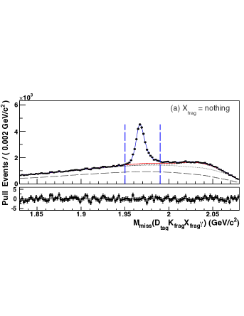
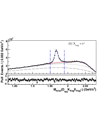
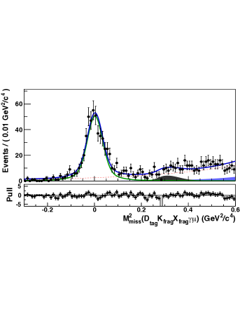
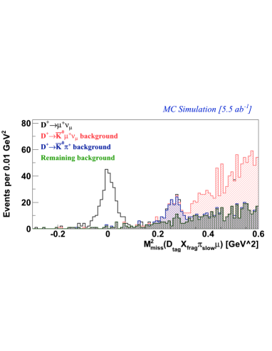
Figure 2: Top: missing mass $\sqrt{(P_{e^{+}}+P_{e^{-}}-P_{\rm tag}-P_{X_{\rm frag}}-P_{\gamma})^{2}}$ from a Belle analysis of $D^{*+}_{s}\!\rightarrow\!D^{+}_{s}\gamma$, $D^{+}_{s}\!\rightarrow\!\mu^{+}\nu$ decays using 913 fb^-1 of data for two fragmentation systems $X_{\rm frag}\!=\!{\rm nothing}$ (left) and $X_{\rm frag}\!=\!\pi^{\pm}$ (right) [15]. Bottom left: missing mass $\sqrt{(P_{e^{+}}+P_{e^{-}}-P_{\rm tag}-P_{X_{\rm frag}}-P_{\gamma}-P_{\mu})^{2}}$ from the same Belle analysis. The peak at zero corresponds to the undetected neutrino from $D^{+}_{s}\!\rightarrow\!\mu^{+}\nu$. Bottom right: missing mass $\sqrt{(P_{e^{+}}+P_{e^{-}}-P_{\rm tag}-P_{X_{\rm frag}}-P_{\pi^{0}}-P_{\mu})^{2}}$ from a Belle II MC study of $D^{*+}\!\rightarrow\!D^{+}\pi^{0},\,D^{+}\!\rightarrow\!\mu^{+}\nu$ decays corresponding to 5.5 ab^-1 of data [16]. A significant signal peak is visible.

3 Semileptonic decays

For semileptonic decays $D\!\rightarrow\!K\ell^{+}\nu$ and $D\!\rightarrow\!\pi\ell^{+}\nu$, the differential partial width to lowest order in $m^{2}_{\ell}$ is [19]

$$\frac{d\Gamma(D\!\rightarrow\!h\ell^{+}\nu)}{dq^{2}} = \frac{G^{2}_{F}}{24\pi^{3}}|f_{+}(q^{2})|^{2}|V_{cx}|^{2}p^{*3}\,,$$ (6)

where $h=K$ or $\pi$, $p^{*}$ is the magnitude of the $K$ or $\pi$ momentum in the $D$ rest frame, and $f_{+}(q^{2})$ is a form factor evaluated at $q^{2}=(P_{D}-P_{h})^{2}=(P_{\ell}+P_{\nu})^{2}$. If $h\!=\!K$, $V_{cx}\!=\!V_{cs}$, while if $h\!=\!\pi$, $V_{cx}\!=\!V_{cd}$. The form factor parameterizes the hadronic matrix element $\langle h|{\cal H}|D\rangle$ and is often modeled with a simple pole: $f_{+}(q^{2})=f_{+}(0)/(1-q^{2}/m^{2}_{\rm pole})$. One thus fits the data at several values of $q^{2}$ to determine the normalization $f_{+}(0)|V_{cx}|$ and the parameter $m_{\rm pole}$.

HFLAV has calculated WA values of $f_{+}(0)|V_{cx}|$ using relevant experimental measurements. The results are [20]

$$f^{K}_{+}(0)|V_{cs}| = 0.7226\,\pm 0.0022\,\pm 0.0026$$ (7)

$$f^{\pi}_{+}(0)|V_{cd}| = 0.1426\,\pm 0.0017\,\pm 0.0008\,,$$ (8)

where the first error is experimental and the second is from theory. The Flavor Lattice Averaging Group [10] quotes results $f^{K}_{+}(0)=0.747\,\pm 0.019$ and $f^{\pi}_{+}(0)=0.666\,\pm 0.029$ as calculated by the HPQCD Collaboration [21, 22]. Inserting these values gives

$$|V_{cs}| = 0.967\,\pm 0.005{\rm\ (exp.)}\,\pm 0.025{\rm\ (theory)}$$ (9)

$$|V_{cd}| = 0.2141\,\pm 0.0029{\rm\ (exp.)}\,\pm 0.0093{\rm\ (theory)}\,.$$ (10)

These values have smaller experimental errors than those obtained from $D^{+}_{(s)}\!\rightarrow\!\ell^{+}\nu$ decays, but the theory errors are larger. This reflects the fact that experiments reconstruct much larger samples of semileptonic decays than purely leptonic decays, but lattice QCD calculations of $f_{+}(0)$ are less precise than calculations of $f_{D_{(s)}}$. A comparison of the different methods made by HFLAV is shown in Fig. 3. A recent calculation [23] of the CKM matrix elements using lattice QCD results that account for the $q^{2}$ dependence of $f_{+}$ [24] gives $|V_{cs}|=0.970\,\pm 0.033$ and $|V_{cd}|=0.2341\,\pm 0.0074$. These values are consistent with results (9) and (10).

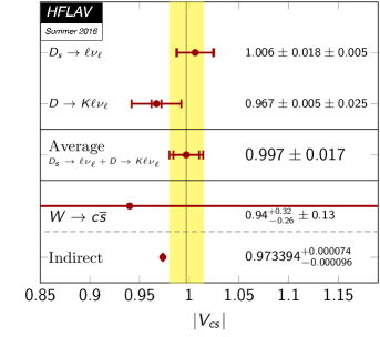
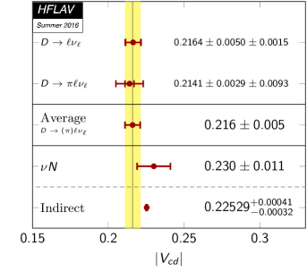
Figure 3: World average (WA) values of $|V_{cs}|$ (left) and $|V_{cd}|$ (right) as calculated by HFLAV using various methods [20].

——————

Belle has measured semileptonic $D^{*+}\!\rightarrow\!D^{0}\pi^{+}$, $D^{0}\!\rightarrow\!(K,\pi)^{-}\ell^{+}\nu$ decays using 282 fb^-1 of data [25]. This analysis proceeds in four steps as done for the Belle $D^{+}_{s}\!\rightarrow\!\ell^{+}\nu$ analysis:

1. a $D^{(*)0}$ or $D^{(*)+}$ decay is reconstructed on the tag-side of an event.

2. a fragmentation system $X_{\rm frag}$ is constructed from remaining $\pi^{\pm}$ tracks, $K^{\pm}$ tracks (an even number), and $\pi^{0}$ candidates. The missing mass $M_{\rm miss}=\sqrt{(P_{e^{+}}+P_{e^{-}}-P_{\rm tag}-P_{X_{\rm frag}})^{2}}$ is calculated, and a kinematic fit is performed subject to the constraint $M_{\rm miss}=M(D^{*})$. The resulting confidence level of the fit is required to be $>\!0.1$%, which corresponds to $M_{\rm miss}$ being within $3.3\sigma$ of $M(D^{*})$.

3. a low-momentum $\pi^{+}$ is selected from among remaining tracks, presumably originating from $D^{*+}\!\rightarrow\!D^{0}\pi^{+}$, and the missing mass $M^{\prime}_{\rm miss}=\sqrt{(P_{e^{+}}+P_{e^{-}}-P_{\rm tag}-P_{X_{\rm frag}}-P_{\pi^{+}})^{2}}$ is calculated. A kinematic fit subject to the constraint $M^{\prime}_{\rm miss}=M(D^{0})$ is performed, and the resulting confidence level is required to be $>\!0.1$%. The $M^{\prime}_{\rm miss}$ distribution is fitted to obtain an inclusive $D^{0}$ signal yield.

4. a $K^{-}$ or $\pi^{-}$ track, and also a $\mu^{+}$ or $e^{+}$ track, are required. No additional (signal candidate) tracks are allowed. The missing mass squared $(P_{e^{+}}+P_{e^{-}}-P_{\rm tag}-P_{X_{\rm frag}}-P_{\pi^{+}}-P_{\ell^{+}}-P_{(K,\pi)^{-}})^{2}$ is calculated. For signal decays this quantity should equal $|m_{\nu}|^{2}$, and thus it is required to be $<\!0.05$ GeV²/$c^{4}$.

The signal yields are obtained after subtracting backgrounds. The results are $2567\pm 52\,{\rm(stat.)}\pm 26\,{\rm(syst.)}$ $D^{0}\!\rightarrow\!K^{-}\ell^{+}\nu$ decays, and $232\pm 17\,{\rm(stat.)}\pm 7\,{\rm(syst.)}$ $D^{0}\!\rightarrow\!\pi^{-}\ell^{+}\nu$ decays.

This method can also be used at Belle II. As the Belle measurement was statistics- rather than systematics-limited, we simply scale the event yields obtained by Belle by the ratio of luminosities. The results are 455000 $D^{0}\!\rightarrow\!K^{-}\ell^{+}\nu$ decays and 41100 $D^{0}\!\rightarrow\!\pi^{-}\ell^{+}\nu$ decays in 50 ab^-1 of Belle II data. An MC study of semileptonic decays in Belle II [16] confirms that these analyses should have very low backgrounds and be statistics limited; see Fig. 4.

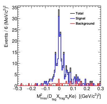
Figure 4: Missing mass squared $(P_{e^{+}}+P_{e^{-}}-P_{\rm tag}-P_{X_{\rm frag}}-P_{\pi^{+}}-P_{K^{-}}-P_{e^{+}})^{2}$ from a Belle II MC study of $D^{*+}\!\rightarrow\!D^{0}\pi^{+},\,D^{0}\!\rightarrow\!K^{-}e^{+}\nu$ decays corresponding to 1 ab^-1 of data [16]. The peak at zero results from the undetected neutrino. For this study only a single tag mode ($D^{0}\!\rightarrow\!K^{-}\pi^{+}$) and a single fragmentation system ($X_{\rm frag}\!=\!\pi^{\pm}$) were reconstructed.

4 $D^{0}\!\rightarrow\!\{{\rm nothing}\}$ decays

In addition to measuring leptonic and semileptonic decays, Belle II can search for the flavor-changing neutral current decay $D^{0}\!\rightarrow\!\nu\bar{\nu}$, or more empirically, $D^{0}\!\rightarrow\!\{{\rm nothing}\}$. The SM rate is negligibly small ($1.1\times 10^{-30}$ [26]), and thus any evidence for this decay would indicate new physics. Belle searched for this decay using 924 fb^-1 of data [27], and an analysis at Belle II would proceed in a similar manner. As done for the Belle analyses of leptonic and semileptonic decays, this analysis first reconstructs a tag-side $D^{(*)}$ decay. It then identifies a $\pi^{+}$ candidate originating from a signal-side $D^{*+}\!\rightarrow\!D^{0}\pi^{+}$ decay; all remaining tracks are considered the fragmentation system $X_{\rm frag}$. The missing mass $\sqrt{(P_{e^{+}}+P_{e^{-}}-P_{\rm tag}-P_{X_{\rm frag}})^{2}}$ is calculated and required to be near $M^{2}(D^{*})$. The signal yield is calculated by simultaneously fitting two distributions: the “$D^{0}$ missing mass” $\sqrt{(P_{e^{+}}+P_{e^{-}}-P_{\rm tag}-P_{X_{\rm frag}}-P_{\pi^{+}})^{2}}$, and the distribution of excess energy deposited in the electromagnetic calorimeter (ECL), i.e., energy clusters unassociated with any track. These distributions are shown in Fig. 5. No signal above background is observed, and an upper limit $B(D^{0}\!\rightarrow\!\nu\bar{\nu})<9.4\times 10^{-5}$ at 90% C.L. is obtained. The size of the inclusive $D^{0}\!\rightarrow\!\{{\rm nothing}\}$ sample is $694670\,^{+1490}_{-1560}$ events. Scaling this yield by the ratio of Belle and Belle II luminosities gives $38\times 10^{6}$ inclusive $D^{0}$ decays in 50 ab^-1 of Belle II data. Scaling the Belle single-event-sensitivity for $D^{0}\!\rightarrow\!\{{\rm nothing}\}$ by a factor of $\sqrt{50/0.924}$ (the argument is the ratio of luminosities) implies a Belle II upper limit of $1.3\times 10^{-5}$ at 90% C.L.

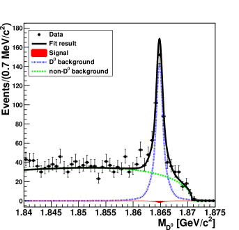
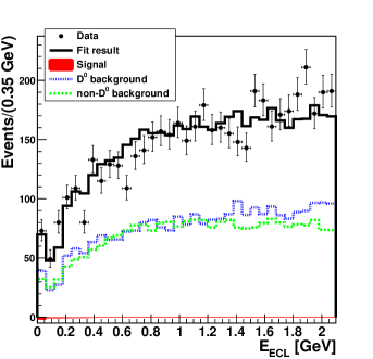
Figure 5: Final $D^{*+}\!\rightarrow\!D^{0}\pi^{+},\,D^{0}\!\rightarrow\!\nu\bar{\nu}$ candidate sample from a Belle analysis of 924 fb^-1 of data [27]. Left: missing mass $\sqrt{(P_{e^{+}}+P_{e^{-}}-P_{\rm tag}-P_{X_{\rm frag}}-P_{\pi^{+}})^{2}}$. Right: excess energy deposited in the electromagnetic calorimeter (ECL), i.e., ECL energy unassociated with any track. The $D^{0}\!\rightarrow\!\nu\bar{\nu}$ signal yield (shown in red) is obtained by simultaneously fitting both distributions.

5 Summary

Belle II will measure leptonic $D^{+}_{(s)}\!\rightarrow\!\ell^{+}\nu$ decays and semileptonic $D^{0}_{(s)}\!\rightarrow\!(K,\pi)^{-}\ell^{+}\nu$ decays using methods developed and refined at Belle and BaBar. In this paper we have reviewed several Belle analyses of these decays and used the results to estimate the sensitivity of Belle II. As these measurements are dominated by statistical uncertainties, our estimates are based on scaling the Belle signal yields by the ratio of luminosities of Belle and Belle II.

The decays $D^{+}_{s}\!\rightarrow\!\ell^{+}\nu$ and $D^{+}\!\rightarrow\!\ell^{+}\nu$ constrain the products $f_{D_{s}}|V_{cs}|$ and $f_{D}|V_{cd}|$, respectively, and the decays $D\!\rightarrow\!K\ell^{+}\nu$ and $D\!\rightarrow\!\pi\ell^{+}\nu$ constrain the products $f^{K}_{+}(0)|V_{cs}|$ and $f^{\pi}_{+}(0)|V_{cd}|$, respectively. Taking decay constants $f_{D_{s}}$ and $f_{D}$ and form factor normalizations $f^{K}_{+}(0)$ and $f^{\pi}_{+}(0)$ from lattice QCD calculations, one can constrain CKM elements $|V_{cs}|$ and $|V_{cd}|$. In this manner one tests CKM unitarity and the SM paradigm. Current results show consistency with unitarity. As Belle II plans to record 50 ab^-1 of data, i.e., $\sim\!50$ times the sample size recorded by Belle, the resulting errors on $|V_{cs}|,\,|V_{cd}|$ should be reduced by a factor of $\sqrt{50}\approx 7$. Belle II will also search for the flavor-changing neutral-current decay $D^{0}\!\rightarrow\!\nu\bar{\nu}$. The full data set of Belle II should yield 7 times the sensitivity of Belle, and possibly much larger, depending on improvements in detector performance and reconstruction algorithms.

——————

We thank the workshop organizers for hosting a well-run meeting with excellent hospitality. We are grateful to Andreas Kronfeld for reviewing this paper and giving valuable input.

References

- [1] https://www.classe.cornell.edu/Research/CLEO/WebHome.html
- [2] http://bes3.ihep.ac.cn/
- [3] https://belle.kek.jp/
- [4] https://www.slac.stanford.edu/BFROOT/
- [5] https://www.belle2.org/
- [6] Charge-conjugate modes are implicitly included throughout this paper.
- [7] D. Silverman and H. Yao, PRD 38, 214 (1988); J. L Rosner, PRD 42, 3732 (1990); C. H. Chang and Y. Q. Chen, PRD 46, 3845 (1992).
- [8] For a review see: A. Ceccucci, Z. Ligeti, and Y. Sakai, “CKM Quark-Mixing Matrix,” in M. Tanabashi et al. (Particle Data Group), PRD 98, 030001 (2018).
- [9] Y. Amhis et al. (Heavy Flavor Averaging Group), EPJC 77, 895 (2017) [pp. 251-252]. See also the online update at https://hflav.web.cern.ch/.
- [10] S. Aoki et al. (Flavor Lattice Averaging Group), EPJC 77, 112 (2017). See also the online update at http://flag.unibe.ch/2019/.
- [11] A. Bazavov et al. (Fermilab/MILC Collaboration), PRD 90, 074509 (2014).
- [12] N. Carrasco et al. (ETM Collaboration), PRD 91, 054507 (2015).
- [13] A. Bazavov et al. (Fermilab/MILC Collaboration), PRD 98, 074512 (2018).
- [14] http://ckmfitter.in2p3.fr/www/results/plots_eps15/num/ckmEval_results_eps15.html
- [15] A. Zupanc et al. (Belle Collaboration), JHEP 09, 139 (2013).
- [16] E. Kou et al. (Belle II Collaboration), “The Belle II Physics Book,” arXiv:1808.10567, to appear in Progress in Theoretical and Experimental Physics.
- [17] B. I. Eisenstein et al. (CLEOc Collaboration), PRD 78, 052003 (2008).
- [18] M. Ablikim et al. (BESIII Collaboration), PRD 89, 051104(R) (2014).
- [19] G. Amoros, S. Noguera, and J. Portoles, EPJC 27, 243 (2003).
- [20] Y. Amhis et al. (Heavy Flavor Averaging Group), EPJC 77, 895 (2017) [pp. 244-247,253]. See also the online update at https://hflav.web.cern.ch/.
- [21] H. Na et al. (HPQCD Collaboration), PRD 84, 114505 (2011).
- [22] H. Na et al. (HPQCD Collaboration), PRD 82, 114506 (2010).
- [23] L. Riggio, G. Salerno, and S. Simula, EPJC 78, 501 (2018).
- [24] V. Lubicz et al. (ETM Collaboration), PRD 96, 054514 (2017).
- [25] L. Widhalm et al. (Belle Collaboration), PRL 97, 061804 (2006).
- [26] A. Badin and A. A. Petrov, PRD 82, 034005 (2010).
- [27] Y.-T. Lai et al. (Belle Collaboration), PRD 95, 011102(R) (2017).