Stable Bayesian Optimisation via Direct Stability Quantification

Abstract

In this paper we consider the problem of finding stable maxima of expensive (to evaluate) functions. We are motivated by the optimisation of physical and industrial processes where, for some input ranges, small and unavoidable variations in inputs lead to unacceptably large variation in outputs. Our approach uses multiple gradient Gaussian Process models to estimate the probability that worst-case output variation for specified input perturbation exceeded the desired maxima, and these probabilities are then used to (a) guide the optimisation process toward solutions satisfying our stability criteria and (b) post-filter results to find the best stable solution. We exhibit our algorithm on synthetic and real-world problems and demonstrate that it is able to effectively find stable maxima.

1 Introduction

A canonical application of Bayesian optimisation is experimental design. Typically one aims to find the optimal experimental parameters - ratios of chemicals, temperatures etc - that maximise some form of experimental yield or return. Implicit in this task is the assumption of repeatability, specifically that if we run the same experiment twice we will obtain the same result. However in all physical experiments there are limitations (both practical and financial) on how precisely one can control the experimental conditions such as ingredient quality (eg type and quantity of any impurities) or oven temperature, and this intrinsic imprecision will manifest in variability in experimental outcomes. If this variability is small then it may be acceptable, but when it is significant it may represent the difference between a good outcome (for example an alloy that is strong and lightweight for aircraft design) or an unacceptable one.

Similar problems also arise outside of the industrial and experimental setting. [11, 10] observes that when tuning hyperparameters we may see the phenomena of false maxima, which are sharp peaks in the performance surface that may be present when the testing set is small that disappear altogether when the size of the testing set increases. Subsequently a simple Bayesian otimisation for hyper-parameter selection may recommend “optimal” hyper-parameters that refer to “optima” that have no objective reality, being a figment of the (small) training set.

Our aim in this paper is twofold. First we show how (in)stability may be characterised and detected using Gaussian Process models, and secondly we show how Bayesian optimisation may be steered to avoid unstable regions and only report stable optima. We begin by characterising instability in terms of maximal output variation bounds given specified (bound) input perturbations: we call this ${(A,B)}$-stability. We then demonstrate how gradient bounds on the first $p$ derivatives (which we call ${{\mu}_{1:p}}$-stability) may be used as a surrogate for ${(A,B)}$-stability, and how the probability of a function being ${{\mu}_{1:p}}$-stable at a point may be calculated using gradient Gaussian process models. Finally we present two modified acquisition function that may be used in Bayesian optimisation to steer the procedure away from unstable regions and toward stable ones.

1.1 Notation

Sets are written ${\mathbb{A}},{\mathbb{B}},\ldots$; where ${\mathbb{R}}_{+}$ is the positive reals, ${\mathbb{Z}}_{+}=\{1,2,\ldots\}$, ${\mathbb{Z}}_{n}=\{0,1,\ldots,n-1\}$, and $\bar{{\mathbb{R}}}_{+}$ is the non-negative reals. $|{\mathbb{A}}|$ is the cardinality of ${\mathbb{A}}$. Column vectors are bold lower case ${\bf a},{\bf b},\ldots$. Matrices are bold upper case ${\bf A},{\bf B},\ldots$. Element $i$ of vector ${\bf a}$ is $a_{i}$. Element $i,j$ of matrix ${\bf W}$ is $W_{i,j}$. ${\bf a}^{{\rm T}}$ is the transpose, ${\bf a}\otimes{\bf b}$ the Kronecker product, and ${\bf a}^{\otimes p}={\bf a}\otimes\overset{p\;{\rm terms}}{\ldots}\otimes{\bf a}$ the Kronecker power. ${\bf 1}$ a vector of $1$s, ${\bf 0}$ a vector of $0$s, and ${\bf I}$ the identity matrix. ${\nabla}_{\bf x}=[\frac{\partial}{\partial x_{0}}\,\frac{\partial}{\partial x_{1}}\,\ldots\,\frac{\partial}{\partial x_{n-1}}]^{{\rm T}}$. The indicator function is denoted $\mathbbold{1}\left({\tt Q}\right)$ and is $1$ if boolean ${\tt Q}$ is true, $0$ otherwise. Logical conjunction is indicated with $\wedge$. Logical disjunction is indicated with $\vee$. The principle branch of the Lambert $W$-function is denoted $W_{0}$. The PDF and CDF of the standard normal distribution are denoted $\phi$ and $\Phi$, respectively.

2 Background

Bayesian optimisation [3, 7, 18, 6] is an optimisation technique designed for optimising expensive (in terms of economic cost, time etc) functions $f$ in the fewest evaluations possible. A Bayesian optimiser maintains a model of $f$ (usually a Gaussian process, as described shortly). At each iteration $t$ the optimiser selects a sample ${\bf x}_{t}\in{\mathbb{X}}$ to maximise an acquisition function $a_{t}:{\mathbb{X}}\to{\mathbb{R}}$ based on this model. This point is evaluated (often noisily) to obtain $y_{t}=f({\bf x}_{t})+\epsilon_{i}$, the model updated, and the process repeated. Acquisition functions are designed to trade-off exploitation of known-good regions and exploration of unknown ones. Typical acquisition functions include expected improvement (EI) [7], GP-UCB [18] and Predictive Entropy Search (PES) [6].

2.1 Gaussian Processes and Derivatives

A gaussian process $\operatorname{{\mathcal{GP}}}(\mu,K)$ is a distribution on a space of functions with mean $\mu:{\mathbb{R}}^{n}\to{\mathbb{R}}$ and covariance $K:{\mathbb{R}}^{n}\times{\mathbb{R}}^{n}\to{\mathbb{R}}$. Assume $f:{\mathbb{X}}\subseteq{\mathbb{R}}^{n}\to{\mathbb{R}}\sim\operatorname{{\mathcal{GP}}}(0,K({\bf x},{\bf x}^{\prime}))$ is a draw from an unbiased Gaussian process [8, 15]. The posterior of $f$ given ${\mathbb{D}}=\{({\bf x}_{i},y_{i})|y_{i}=f({\bf x}_{i})+\epsilon_{i},\epsilon_{i}\sim{\mathcal{N}}(0,\sigma^{2})\}$ is $f({\bf x})|{\mathbb{D}}\sim{\mathcal{N}}(m_{\mathbb{D}}({\bf x}),\lambda_{\mathbb{D}}({\bf x},{\bf x}))$, where:

$$\begin{array}[]{rl}m_{\mathbb{D}}\!\left({\bf x}\right)&\!\!\!\!={\bf k}^{{\rm T}}\!\left({\bf x}\right)\left({\bf K}+{\sigma}^{2}{\bf I}\right)^{-1}\!{\bf y}\\ \!\!\!\!\!\lambda_{\mathbb{D}}\!\left({\bf x},{\bf x}^{\prime}\right)&\!\!\!\!=K\!\left({\bf x},{\bf x}^{\prime}\right)-{\bf k}^{{\rm T}}\!\left({\bf x}\right)\left({\bf K}+{\sigma}^{2}{\bf I}\right)^{-1}\!{\bf k}\left({\bf x}^{\prime}\right)\!\!\!\!\!\!\!\end{array}$$ (1)

${\bf y},{\bf k}({\bf x})\in{\mathbb{R}}^{|{\mathbb{D}}|}$, ${\bf K}\in{\mathbb{R}}^{|{\mathbb{D}}|\times|{\mathbb{D}}|}$, $k({\bf x})_{i}=K({\bf x},{\bf x}_{i})$, and $K_{i,j}=K({\bf x}_{i},{\bf x}_{j})$.

The gradient of a Gaussian process is an (independent [19]) Gaussian process [13, 14, 17] if the kernel is differentiable, and so on too are higher order gradients of Gaussian processes. In vectorised form, denoting the Kronecker power ${\bf a}^{\otimes q}={\bf a}\otimes\overset{q\;{\rm terms}}{\ldots}\otimes{\bf a}$, the posterior of ${\nabla}_{\bf x}^{\otimes q}f$ given ${\mathbb{D}}$ is ${\nabla}_{\bf x}^{\otimes q}f({\bf x})|{\mathbb{D}}\sim{\mathcal{N}}({\bf m}_{\mathbb{D}}^{(q)}({\bf x}),{{\mbox{\boldmath$\Lambda$}}}_{{\mathbb{D}}}^{(q)}({\bf x},{\bf x}))$, where:

$$\begin{array}[]{rl}{\bf m}_{\mathbb{D}}^{\!(q)}\!\left({\bf x}\right)&\!\!\!\!\!=\!\left({\nabla}_{\bf x}^{\otimes q}{\bf k}^{{\rm T}}\!\left({\bf x}\right)\right)\left({\bf K}+{\sigma}^{2}{\bf I}\right)^{-1}{\bf y}\\ \!\!\!\!\!\!{\mbox{\boldmath$\Lambda$}}_{\mathbb{D}}^{\!(q)}\!\left({\bf x},\!{\bf x}^{\prime}\right)&\!\!\!\!\!=\!\nabla_{\bf x}^{\otimes q}\nabla_{{\bf x}^{\prime}}^{\otimes q}{}^{{\rm T}}\!K\!\left({\bf x},\!{\bf x}^{\prime}\right)\!-\!\left({\nabla}_{\bf x}^{\otimes q}{\bf k}^{{\rm T}}\!\!\left({\bf x}\right)\right)\!({\bf K}+\!\!\!\!\!\!\\ &\!\!\!\ldots+{\sigma}^{2}{\bf I})^{-1}\!\left({\nabla}_{{\bf x}^{\prime}}^{\otimes q}{\bf k}^{{\rm T}}\!\left({\bf x}^{\prime}\right)\right)^{{\rm T}}\end{array}$$ (2)

and we note that:

$$\begin{array}[]{l}{\rm vec}\left(\nabla_{{\bf x}}^{\otimes q}\nabla_{{\bf x}^{\prime}}^{\otimes q{\rm T}}K\left({\bf x},{\bf x}^{\prime}\right)\right)=\left(\nabla_{{\bf x}^{\prime}}^{\otimes q}\otimes\nabla_{{\bf x}}^{\otimes q}\right)K\left({\bf x},{\bf x}^{\prime}\right)\end{array}$$

Relevant gradient calculations for standard $K$ functions can be found in [9]. Alternatively for the isotropic kernels:

$$\begin{array}[]{l}K\left({\bf x},{\bf x}^{\prime}\right)=\kappa\left(\frac{1}{2}\left\|{\bf x}-{\bf x}^{\prime}\right\|_{2}^{2}\right)\end{array}$$

assuming $\kappa$ is differentiable in closed form the following result, along with table 1, may be used to calculate the required derivatives:

Theorem 1

Let $K({\bf x},{\bf x}^{\prime})=\kappa(\frac{1}{2}\|{\bf x}-{\bf x}^{\prime}\|_{2}^{2})$ be an isotropic kernel, where $\kappa$ is $s$-times differentiable. Denote by $\nabla_{{\bf x}^{\ldots}}^{\otimes q}$ a mixed Kronecker derivative of order $q$ (e.g. $\nabla_{{\bf x}^{\ldots}}^{\otimes 2}$ may be $\nabla_{{\bf x}}\otimes\nabla_{{\bf x}}$, $\nabla_{{\bf x}^{\prime}}\otimes\nabla_{{\bf x}^{\prime}}$, $\nabla_{{\bf x}}\otimes\nabla_{{\bf x}^{\prime}}$ or $\nabla_{{\bf x}^{\prime}}\otimes\nabla_{{\bf x}}$), where $\alpha$ is the number of times $\nabla_{{\bf x}^{\prime}}$ appears in $\nabla_{{\bf x}^{\ldots}}^{\otimes q}$. Then $\forall q\in{\mathbb{Z}}_{s+1}$:

$$\begin{array}[]{l}{\nabla_{{\bf x}^{\ldots}}^{\otimes q}K\left({\bf x},{\bf x}^{\prime}\right)=\left(-1\right)^{\alpha}\mathop{\sum}\limits_{i=0}^{\left\lfloor\frac{q}{2}\right\rfloor}{\bf a}_{(i,q)}\left({\bf x}^{\prime}-{\bf x}\right)\kappa^{(q-i)}\left(\frac{1}{2}\left\|{\bf x}-{\bf x}^{\prime}\right\|_{2}^{2}\right)}\end{array}$$

where $\kappa^{(c)}(x)=\frac{\partial^{c}}{\partial x^{c}}\kappa(x)$;

$$\begin{array}[]{rl}{\bf a}_{(i,q)}\left({\bf d}\right)&\!\!\!=\mathop{\sum}\limits_{{\bf j}\in{\mathbb{J}}_{(i,q)}}\;\;\mathop{\otimes}\limits_{k=0}^{q-1}\left\{\begin{array}[]{ll}{{\bf d}}&{{\tt{if}}\;j_{k}=0}\\ {{\mbox{\boldmath$\delta$}}_{j_{k}}}&{\tt otherwise}\\ \end{array}\right.\end{array}$$ (3)

$$\begin{array}[]{l}\scriptstyle{{\mathbb{J}}_{(i,q)}=\{\left.{\bf j}\in{\mathbb{Z}}^{q}\right|\left\{j_{0},j_{1},\ldots,j_{q-1}\right\}=\left\{0,\ldots,0,-1,-1,-2,-2,\ldots,-i,-i\right\}\wedge\ldots}\\ \scriptstyle{\mathop{\operatorname{argmin}}\left\{\left.j_{k}\right|j_{k}=-1\right\}\leq\mathop{\operatorname{argmin}}\left\{\left.j_{k}\right|j_{k}=-2\right\}\leq\ldots\leq\mathop{\operatorname{argmin}}\left\{\left.j_{k}\right|j_{k}=-i\right\}\}}\end{array}$$

and we have used the symbolic notation (where ${\bf i}\in{\mathbb{Z}}_{n}^{q}$ is a multi-index, noting that ${\mbox{\boldmath$\delta$}}_{l}$’s appear in pairs in ${\bf a}_{(i,q)}$ $\forall l=-1,-2,\ldots,-i$):

$$\begin{array}[]{l}{(\overbrace{{\overset{{a\;{\tt{terms}}}}{\ldots}\otimes{\mbox{\boldmath$\delta$}}_{l}\otimes\ldots}}^{{b\;{\tt{terms}}}}\otimes{\mbox{\boldmath$\delta$}}_{l}\otimes\ldots)_{\bf i}=(\delta_{i_{a},i_{b}}(\overbrace{{\overset{{a\;{\tt{terms}}}}{\ldots}\otimes{\bf 1}\otimes\ldots}}^{{b\;{\tt{terms}}}}\otimes{\bf 1}\otimes\ldots))_{\bf i}}\end{array}$$

Proof:

The complete proof of this theorem is presented in the appendix. The proof begins by assuming that $\alpha=0$ (that is, $\nabla_{{\bf x}^{\prime}}$ does not appear in the Kronecker gradient, so $\nabla_{{\bf x}^{\ldots}}^{\otimes q}K({\bf x},{\bf x}^{\prime})=\nabla_{{\bf x}}^{\otimes q}K({\bf x},{\bf x}^{\prime})$) and proving the special case inductively. The general case $\alpha\geq 0$ follows by observing the sign anti-symmetry of the gradients with respect to ${\bf x}$ and ${\bf x}^{\prime}$. $\square$

3 Problem Statement

Let $f:{\mathbb{X}}\to{\mathbb{R}}_{+}$. We assume that $f$ may be evaluated (with noise and significant expense) but that its derivatives may not. Our aim is to find the stable maxima:

$$\begin{array}[]{rl}{\bf x}^{*}=\mathop{\operatorname{argmax}}\limits_{{\bf x}\in{\mathbb{S}}}f\left({\bf x}\right)\end{array}$$ (4)

where ${\mathbb{S}}\subseteq{\mathbb{X}}$ is the stable subset of ${\mathbb{X}}$. To achieve this we must (a) quantify what we mean by stability in practical terms, and (b) incorporate this into the acquisition function used by the Bayesian optimiser.

3.1 Assumptions

For the purposes of this paper we assume:

1. ${\mathbb{X}}\subset{\mathbb{R}}^{n}$ compact, $\|{\bf x}-{\bf x}^{\prime}\|_{2}\leq M$ $\forall{\bf x},{\bf x}^{\prime}\in{\mathbb{X}}$.

2. $f:{\mathbb{X}}\subseteq{\mathbb{R}}^{n}\to{\mathbb{R}}_{+}\sim\operatorname{{\mathcal{GP}}}(0,K({\bf x},{\bf x}^{\prime}))$.

3. $\|f\|_{{\mathbb{H}}_{K}}\leq G$, where $\|\cdot\|_{{\mathbb{H}}_{K}}$ is the reproducing kernel Hilbert space norm.

4. $K({\bf x},{\bf x}^{\prime})=\kappa(\frac{1}{2}\|{\bf x}-{\bf x}^{\prime}\|_{2}^{2})$ is isotropic kernel (covariance), $\kappa$ is completely monotone, positive, $s$-times differentiable, and there exist $L^{\uparrow}\geq L^{\downarrow}\in{\mathbb{R}}_{+}$, $\Delta_{r}:{\mathbb{R}}_{+}\to{\mathbb{R}}_{+}$ non-decreasing such that:

   $$\begin{array}[]{l}L^{\downarrow q}\kappa\left(r\right)\leq\left|\kappa^{(q)}\left(r\right)\right|\leq L^{\uparrow q}\kappa\left(r\right)\;\forall q\in{\mathbb{Z}}_{s+1}\\ \left|\kappa\left(r+\delta r\right)-\mathop{\sum}\limits_{q\in{\mathbb{Z}}_{s+1}}\frac{1}{q!}\delta r^{q}\kappa^{(q)}\left(r\right)\right|\leq\Delta_{r}\left(\delta r\right)\end{array}$$

   and we define the overall Taylor bound for $\kappa$ as:

   $$\begin{array}[]{l}\Delta\left(\delta r\right)=\mathop{\sup}\limits_{r\in\left[0,\frac{1}{2}M^{2}\right)}\frac{\Delta_{r}\left(\delta r\right)}{\kappa\left(r\right)}\end{array}$$

Of these assumptions only assumption 4 is the only non-trivial. We have considered only isotropic kernels as these represent the most common kernels in the Gaussian process literature, and restricted our choice to positive (valued) kernels (excluding for example the wave kernel) rather than Bernstein to enable us to construct various bounds on the remainder of $f$. The parameters $L^{\uparrow},L^{\downarrow}$ (and their existance and finiteness) is required to allow us to bound the Taylor expansion of $f$, which forms the basis of our defintion of stability, while the non-decreasing (in $\delta r$) bound on the remainder of the Taylor expansion is a convenience factor allowing us to use a richer range of (non-infinitely-differentiable) kernels. Examples of kernels satisfying the conditions of this assumption are presented in table 1.

On a technical point, we note that the remainder bounds $\Delta_{r}$, $\Delta$ can be difficult to calculate in closed form. As discussed in the appendix, if a (tight) closed-form bound is not available then these terms may be approximated using Monte-Carlo simulation [4]. Specifically:

$$\begin{array}[]{r}{\Delta_{r}\left(\delta r\right)\approx\max\{\left.E_{r}\left(\delta r\right),E_{r}\left(s_{i}\right)\right|s_{0},s_{1},\ldots s_{R_{A}-1}\sim{\mathcal{U}}\left(0,\delta r\right)\}}\end{array}$$ (5)

where:

$$\begin{array}[]{l}E_{r}\left(\delta r\right)=\left|\kappa\left(r+\delta r\right)-\mathop{\sum}\limits_{q\in{\mathbb{Z}}_{s+1}}\frac{1}{q!}\delta r^{q}\kappa^{(q)}\left(r\right)\right|\end{array}$$

is a tight bound on the absolute remainder of the Taylor expansion of $\kappa$, and samples are drawn to ensure $\Delta_{r}(\delta r)$ is increasing with respect to $\delta r$. Obviously more samples $R_{A}$ will give a more accurate bound, while fewer samples will be faster to evaluate. Likewise:

$$\begin{array}[]{r}{\Delta\left(\delta r\right)\approx\max\{\left.\frac{\Delta_{r}\left(\delta r\right)}{\kappa\left(r\right)}\right|r_{0},r_{1},\ldots,r_{R_{B}-1}\sim{\mathcal{U}}\left(0,\frac{1}{2}M^{2}\right)\}}\end{array}$$ (6)

where the total number of samples required for this approximation is $R_{A}R_{B}$. We note that this need only be calculated twice in our algorithm, so it is feasible to use a larger number of samples to ensure accuracy. See appendix for further discussion and relevant derivations.

Kernel	Derivatives	$s$
RBF	$\!\!\!\begin{array}[]{l}\kappa_{(\gamma)}\left(r\right)=e^{-\frac{1}{\gamma^{2}}r}\\ \kappa_{(\gamma)}^{(q)}\left(r\right)=\left(-\frac{1}{\gamma^{2}}\right)^{q}e^{-\frac{1}{\gamma^{2}}r}\\ \end{array}\!\!\!$	$\infty$	$\!\!\!\begin{array}[]{l}L_{(\gamma)}^{\uparrow}=L_{(\gamma)}^{\downarrow}=\frac{1}{\gamma^{2}}\\ \Delta_{(\gamma)r}\left(\delta r\right)=\Delta_{(\gamma)}\left(\delta r\right)=0\\ \end{array}\!\!\!$
$\frac{1}{2}$-Matern	$\!\!\!\begin{array}[]{l}\kappa_{(\frac{1}{2},\rho)}\left(r\right)=e^{-\frac{\sqrt{2r}}{\rho}}\\ \end{array}\!\!\!$	$0$	$\!\!\!\begin{array}[]{l}L_{(\frac{1}{2},\rho)}^{\uparrow}=\sqrt{\frac{1}{2}}\frac{1}{2\rho}\\ L_{(\frac{1}{2},\rho)}^{\downarrow}=0.3764\sqrt{\frac{1}{2}}\frac{1}{2\rho}\\ \Delta_{(\frac{1}{2},\rho)r}\left(\delta r\right),\Delta_{(\frac{1}{2},\rho)}\left(\delta r\right)={}^{*}\\ \end{array}\!\!\!$
$\frac{3}{2}$-Matern	$\!\!\!\begin{array}[]{l}\kappa_{(\frac{3}{2},\rho)}\left(r\right)=\left(1+\frac{\sqrt{6r}}{\rho}\right)e^{-\frac{\sqrt{6r}}{\rho}}\\ \kappa_{(\frac{3}{2},\rho)}^{(1)}\left(r\right)=-\frac{\sqrt{3}}{\sqrt{2}\rho}\kappa_{(\frac{1}{2},\rho)}\left(r\right)\\ \end{array}\!\!\!$	$1$	$\!\!\!\begin{array}[]{l}L_{(\frac{3}{2},\rho)}^{\uparrow}=\mathop{\max}\limits_{c\in\{0,1\}}\left\{1,\frac{\kappa_{d+\frac{1}{2}-c}\left(\frac{1}{2}M^{2}\right)}{\kappa_{d+\frac{1}{2}}\left(\frac{1}{2}M^{2}\right)}\right\}\sqrt{\frac{3}{2}}\frac{1}{2\rho}\\ L_{(\frac{3}{2},\rho)}^{\downarrow}=0.7528\sqrt{\frac{3}{2}}\frac{1}{2\rho}\\ \Delta_{(\frac{3}{2},\rho)r}\left(\delta r\right),\Delta_{(\frac{3}{2},\rho)}\left(\delta r\right)={}^{*}\\ \end{array}\!\!\!$
$\frac{5}{2}$-Matern	$\!\!\!\begin{array}[]{l}\kappa_{(\frac{5}{2},\rho)}\left(r\right)=\left(1+\frac{\sqrt{10r}}{\rho}+\frac{10r}{3\rho^{2}}\right)e^{-\frac{\sqrt{10r}}{\rho}}\\ \kappa_{(\frac{5}{2},\rho)}^{(1)}\left(r\right)=-\frac{\sqrt{5}}{3\sqrt{2}\rho}\kappa_{(\frac{3}{2},\rho)}\left(r\right)\\ \kappa_{(\frac{5}{2},\rho)}^{(2)}\left(r\right)=\frac{5}{6\rho^{2}}\kappa_{(\frac{1}{2},\rho)}\left(r\right)\\ \end{array}\!\!\!$	$2$	$\!\!\!\begin{array}[]{l}L_{(\frac{5}{2},\rho)}^{\uparrow}=\mathop{\max}\limits_{c\in\{0,1,2\}}\left\{1,\frac{\kappa_{d+\frac{1}{2}-c}\left(\frac{1}{2}M^{2}\right)}{\kappa_{d+\frac{1}{2}}\left(\frac{1}{2}M^{2}\right)}\right\}\sqrt{\frac{5}{2}}\frac{1}{2\rho}\\ L_{(\frac{5}{2},\rho)}^{\downarrow}=0.5018\sqrt{\frac{5}{2}}\frac{1}{2\rho}\\ \Delta_{(\frac{5}{2},\rho)r}\left(\delta r\right),\Delta_{(\frac{5}{2},\rho)}\left(\delta r\right)={}^{*}\\ \end{array}\!\!\!$

Table 1: Relevant standard isotropic kernels. In this table $K({\bf x},{\bf x}^{\prime})=\kappa(\frac{1}{2}\|{\bf x}-{\bf x}^{\prime}\|_{2}^{2})$, $s$ is the differentiability of $\kappa$, $\kappa^{(q)}(r)=\frac{\partial^{q}}{\partial r^{q}}\kappa(r)$ is the $q^{\rm th}$ derivative ($q\in{\mathbb{Z}}_{s+1}$) of $\kappa$, $L^{\uparrow},L^{\downarrow}$ relate to the effective length-scales, and $\Delta_{r}$, $\Delta$ are the Taylor remainder bounds (bounds labelled ^∗ may be calculated numerically using (5) and (6)).

3.2 Related Work

The works most closely related to the present work are unscented Bayesian optimisation [12] and stable Bayesian optimisation [11, 10]. Both of these works attempt to find stability in terms of input noise by translating it to output (target) noise. [12] does this using the unscented transformation, while [11, 10] constructs a new acquisition function combining the effects of epistemic variance (“standard” variance in the output due to limited samples and noisy measurements) and aleatoric variance due to input perturbations translated into output through the objective function. Thus unstable regions of the objective function become regions of high uncertainty, which the algorithm may subsequently avoid. However there is no guarantee that such approaches will avoid unstable regions, particularly those that combine instability and particularly high (relative) return, so variability of results may still be a problem.

4 Stability - Definition and Quantification

In this section we present two definitions of stability, ${(A,B)}$-stability and ${{\mu}_{1:p}}$-stability. ${(A,B)}$-stability is defined in terms of the sensitivity of the output to variation in the input - the smaller $|f({\bf x})-f({\bf x}+\delta{\bf x})|$ is for bounded $\delta{\bf x}$, the more stable $f$ is at ${\bf x}\in{\mathbb{X}}$. This is a practical definition for the experimenter, but is difficult to quantify in practice. Alternatively, ${{\mu}_{1:p}}$-stability defines stability in terms of gradients (to order $p$). This is not as useful for the experimenter, but, as we will show, may be readily quantified using gradient Gaussian processes. In this section we will relate these two definitions and demonstrate that ${{\mu}_{1:p}}$-stability may be used as a surrogate for ${(A,B)}$-stability, allowing the experimenter to specify stability constraints in the more practical ${(A,B)}$-stable form and then enforce them in terms of the more practical ${{\mu}_{1:p}}$-stability form.

4.1 Defining Stability

${(A,B)}$-stability is defined as follows:

Definition 1 (${(A,B)}$-stability)

Let $A,B\in{\mathbb{R}}_{+}$. We say that $f$ is ${(A,B)}$-stable at point ${\bf x}\in{\mathbb{X}}$ if $|f({\bf x}+\delta{\bf x})-f({\bf x})|\leq A$ $\forall\delta{\bf x}:\|\delta{\bf x}\|_{2}\leq B$. The set of all ${(A,B)}$-stable points for $f$ is denoted ${\mathbb{S}}_{{(A,B)}}$.

Intuitively a function $f$ is ${(A,B)}$-stable at ${\bf x}$ if input perturbation of magnitude less than $B$ leads to output variation of magnitude less than $A$.

Alternatively, stability may be defined by bounding the derivatives of $f$ up to some order $p$. This is motivated by the observation that, if the derivative $\nabla_{\bf x}f({\bf x})$ is large then small changes in ${\bf x}$ will lead to large changes in $f({\bf x})$; and if the vectorised Hessian $\nabla_{\bf x}^{\otimes 2}f({\bf x})$ is large then, even if the gradient is small at ${\bf x}$, small (finite) changes in ${\bf x}$ may nevertheless cause us to “fall off” the sharp (unstable) peak at this point. Thus we would like to label regions with large derivatives $\nabla_{\bf x}f({\bf x})$ or large vectorised Hessian $\nabla_{\bf x}^{\otimes 2}f({\bf x})$ as unstable; hence, generalising to arbitrary order, we define ${{\mu}_{1:p}}$-stability by:

Definition 2 (${{\mu}_{1:p}}$-stability)

Let ${\mu},B\in{\mathbb{R}}_{+}$ and $p\in{\mathbb{Z}}_{+}$. We say that $f$ is ${{\mu}_{1:p}}$-stable at point ${\bf x}$ if $\forall q\in{\mathbb{Z}}_{p}+1$:

$$\begin{array}[]{l}\frac{B^{q}}{q!}\left\|\nabla_{\bf x}^{\otimes q}f\left({\bf x}\right)\right\|_{2}\leq{\mu}\end{array}$$

The set of all ${{\mu}_{1:p}}$-stable points for $f$ is denoted ${\mathbb{S}}_{{{\mu}_{1:p}}}$. We also say that $f$ is ${{\mu}_{q}}$-stable at ${\bf x}$ for a given $q\in{\mathbb{Z}}_{+}$ if the gradient bound is met for the $q$ specified.

4.2 Connection Between ${(A,B)}$- and ${{\mu}_{1:p}}$-Stability

The forms of stability we have defined (${(A,B)}$-stability and ${{\mu}_{1:p}}$-stability) are related through the following key result, which (a) shows that ${(A,B)}$-stability is equivalent to ${{\mu}_{1:p}}$-stability in the limit $p\to\infty$ for appropriately conditions on $f$ and selected $\mu$ and (b) suggests how the paremeters $p$ and ${\mu}$ may be selected given $A,B\in{\mathbb{R}}_{+}$ and the specifics of the kernel $K$ ($s$, $L_{(q)}$, $\Delta_{r}(\delta r)$ and $\Delta(\delta r)$, as per section 3.1).

Theorem 2

Let $A,B\in{\mathbb{R}}_{+}$, $s\in{\mathbb{Z}}_{+}$. Under the default assumptions, suppose the remainders of $f({\bf x}+\delta{\bf x})$ Taylor expanded about ${\bf x}\in{\mathbb{X}}$ to order $q$ satisfy the bound $|R_{q:{\bf x}}(\delta{\bf x})|\leq U_{q}(B)$ $\forall\delta{\bf x},\|\delta{\bf x}\|_{2}\leq B$. Define:

$$\begin{array}[]{l}{\mathbb{P}}=\left\{p\in{\mathbb{Z}}_{s}+1\left|U_{p}\left(B\right)\leq A\right.\right\}\\ \end{array}$$

If ${\mathbb{P}}\neq\emptyset$, $p\in{\mathbb{P}}$, and ${{{\mu}^{\pm}}}=(A\pm U_{p}(B))$ then, using ${{\mu}^{+}_{1:p}}$-stability and ${{\mu}^{-}_{1:p}}$-stability to denote ${{\mu}_{1:p}}$-stability with, respectively, ${\mu}={{\mu}^{+}}$ and ${\mu}={{\mu}^{-}}$, we have:

$$\begin{array}[]{l}{\mathbb{S}}_{{{\mu}^{-}_{1:p}}}\subseteq{\mathbb{S}}_{{(A,B)}}\subseteq{\mathbb{S}}_{{{\mu}^{+}_{1:p}}}\end{array}$$

Proof:

This follows from the definitions in a straightforward manner applying standard inequalitites. See appendix for details. $\square$

This theorem suggests that we may use ${{\mu}_{1:p}}$-stability as a proxy for ${(A,B)}$-stability, and suggests a range ${\mu}\in[{{\mu}^{-}},{{\mu}^{+}}]$ of choices for ${\mu}$ to approximate ${(A,B)}$-stability given $A,B\in{\mathbb{R}}_{+}$, as shown for example in figure 1. This is desirable because the derivatives of a Gaussian Process are Gaussian Processes (to order $s$, see section 2.1), which will allow us to directly calculate the probability that $f$ is ${{\mu}_{1:p}}$-stable at a point ${\bf x}$ given observations ${\mathbb{D}}$, which allows us to quantify the expected gain for a particular recommendation and thus construct a sensible acquisition function for our Bayesian optimiser. Note that:

• Smaller ${\mu}$ (e.g. ${\mu}={{\mu}^{-}}$) defines a conservative approximation excluding marginally stable points, while larger ${\mu}$ (e.g. ${\mu}={{\mu}^{+}}$) defines a more liberal approximation possibly including marginally unstable points.

• If the Taylor expansion of $\kappa$ converges (so $U_{q}(B)$ decreases with $q$) then larger $p$ values will result in better approximation of ${(A,B)}$-stability. However this must be balanced against the computational cost of calculating means and variances of $n^{p}$-dimensional ($p^{\rm th}$-order derivative) Gaussian processes. In practice we found this to be of little concern as $p\leq 2$ typically suffices, which bounds the gradient and Hessian, where bounding the gradient excludes unstable maxima on the boundaries of ${\mathbb{X}}$, and bounding the Hessian excludes unstable, quadratic-type maxima.

The convergence rate of the Taylor expansion of $f$ depends on the isotropic kernel function $K$ of the Gaussian process from which $f$ was drawn, as quantified by the following theorem (proven in the appendix), where for clarity we consider the simplified case $s=\infty$, $\Delta(r)=0$ (the more general case is presented in the appendix):

Theorem 3

Under the default assumptions $|f({\bf x})|\leq F$ $\forall{\bf x}\in{\mathbb{X}}$, where:

$$\begin{array}[]{l}F=\kappa\left(0\right)\sqrt{\frac{1}{\Gamma\left(\frac{n}{2}+1\right)}\left(\frac{\sqrt{\pi}M}{2}\right)^{n}}G\end{array}$$

and the remainders of $f({\bf x}+\delta{\bf x})$ Taylor expanded around ${\bf x}\in{\mathbb{X}}$ to order $q\in{\mathbb{Z}}_{s}+1$ are bounded by:

$$\begin{array}[]{r}{\left|R_{q:{\bf x}}\left(\delta{\bf x}\right)\right|\leq\frac{D}{\sqrt{(q+1)!}}\frac{\left(\sqrt{2L^{\uparrow}}B\right)^{q+1}\!\!\!-\left(\sqrt{2L^{\uparrow}}B\right)^{s+1}}{1-\sqrt{2L^{\uparrow}}B}F}\\ \end{array}$$

$\forall\delta{\bf x}:\|\delta{\bf x}\|_{2}\leq B<\frac{1}{\sqrt{2L^{\uparrow}}}$, where:

$$\begin{array}[]{l}D=0.816\pi^{\frac{1}{4}}e^{\frac{1}{2}\left(\sqrt{L^{\uparrow}}M\right)^{2}}+\ldots\\ \frac{L^{\uparrow}-L^{\downarrow}}{L^{\uparrow}}\mathop{\sum}\limits_{i=0}^{s}\mathop{\sum}\limits_{i=0}^{\left\lfloor\frac{1}{2}\left\lfloor\frac{q}{2}\right\rfloor\right\rfloor}\frac{\sqrt{q!}}{2^{2i}(2i)!(q-4i)!}\left(\sqrt{L^{\uparrow}-L^{\downarrow}}M\right)^{q-4i}\\ \end{array}$$

Moreover $|R_{p:{\bf x}}(\delta{\bf x})|\leq A$ $\forall p\geq p_{\rm min}$, where:

$$\begin{array}[]{r}{p_{\rm min}=\max\Big{\{}1,\Big{\lceil}\left(\sqrt{2L^{\uparrow}}B\right)^{2}\exp\Big{(}1+W_{0}\Big{(}\frac{2}{e\left(\sqrt{2L^{\uparrow}}B\right)^{2}}\log\ldots}\\ {\ldots\left(\frac{1}{\sqrt{\sqrt{2\pi}}}\frac{DF}{A}\frac{1}{1-\sqrt{2L^{\uparrow}}B}\right)\Big{)}\Big{)}-1\Big{\rceil}\Big{\}}}\\ \end{array}$$

where $W_{0}$ is the principle branch of the Lambert $W$-function.

Proof:

A proof is given in the appendix. Several steps are required. As preliminary, we show that the number of terms in the gradients $\nabla_{\bf x}^{\otimes q}K({\bf x},{\bf x}^{\prime})$ is equal to the number of terms in the Hermite polynomial $H_{q}$. This is leveraged to construct a bound on the remainders of the Taylor expansion of $\kappa$. Noting that $f$ is in a reproducing kernel Hilbert space, the bound on the remainder of $\kappa$ is used to bound the remainder of the Taylor expansion of $f$. Finally Stirlings approximation is used to find $p_{\rm min}$. $\square$

This theorem provides the details required to use ${{\mu}_{1:p}}$-stability as a proxy for ${(A,B)}$-stability, as suggested by theorem 2. In particular, it suggests that we choose $p=p^{\rm rec}$ and ${\mu}\in[{{\mu}^{-}},{{\mu}^{+}}]$, where, using the constants in the theorem, and provided $B<\frac{1}{\sqrt{2L}}$:

$$\begin{array}[]{l}\!\!\!\!\!\!\!\!\!\begin{array}[]{r}{p^{\rm rec}=\max\max\Big{\{}1,\Big{\lceil}\left(\sqrt{2L^{\uparrow}}B\right)^{2}\exp\Big{(}1+W_{0}\Big{(}\frac{2}{e\left(\sqrt{2L^{\uparrow}}B\right)^{2}}\log\ldots}\\ {\ldots\left(\frac{1}{\sqrt{\sqrt{2\pi}}}\frac{DF}{A}\frac{1}{1-\sqrt{2L^{\uparrow}}B}\right)\Big{)}\Big{)}-1\Big{\rceil}\Big{\}}}\\ \end{array}\!\!\!\!\!\!\!\!\!\\ \!\!\!\!\!\!\!\!\!\begin{array}[]{r}{{{{\mu}^{\pm}}}=A\pm\frac{D}{\sqrt{(q+1)!}}\frac{\left(\sqrt{2L^{\uparrow}}B\right)^{q+1}\!\!\!-\left(\sqrt{2L^{\uparrow}}B\right)^{s+1}}{1-\sqrt{2L^{\uparrow}}B}F}\\ \end{array}\!\!\!\!\!\!\!\!\!\end{array}$$ (7)

where $F=\kappa(0)\sqrt{\frac{1}{\Gamma(\frac{n}{2}+1)}(\frac{\sqrt{\pi}M}{2})^{n}}G$. Note that the restriction $B<{1}/{\sqrt{2L^{\uparrow}}}$ on input variation is actually a requirement that the input variation be less than an amount proportional to the (effective) length-scale of the kernel $K$.

Finally we note that in practice we have observed that it is almost never necessary to test ${{\mu}_{1:p}}$-stability past $3^{\rm rd}$-order (or even $2^{\rm nd}$ order) in most cases when using an RBF kernel. This appears to be due to two factors:

• The scaled gradients $\frac{B^{q}}{q!}\nabla_{\bf x}^{\otimes q}f({\bf x})$ taper off much more quickly than the bounds in theorem 3 may suggest, presumably due to the number of approximations (upper bounds) required to obtain the said bounds. For example in figure 1 we see that by $3^{\rm rd}$-order the scaled gradients fall well within the bounds of ${{\mu}_{1:p}}$-stability.

• Even if a higher-order derivative fails to meet the bound requirement $\|\frac{B^{q}}{q!}\nabla_{\bf x}^{\otimes q}f({\bf x})\|_{2}\leq{\mu}$, usually a lower-order derivative will also fail to meet this bound, rendering the (more computationally expensive) higher-order test superfluous.

Next we consider how the stability of a point may be quantified when the derivatives are approximated using the derivatives of the Gaussian process model of $f$.

4.3 Quantifying Stability

We now show how the derivatives of the Gaussian process model of $f$ may be used to calculate the posterior probability that $f$ is ${{\mu}_{1:p}}$-stable at ${\bf x}\in{\mathbb{X}}$. Using the notation of section 2.1, given ${\mathbb{D}}=\{({\bf x}_{i},y_{i})|y_{i}=f({\bf x}_{i})+\epsilon_{i},\epsilon_{i}\sim{\mathcal{N}}(0,\sigma^{2})\}$:

$$\begin{array}[]{rl}\left.f\left({\bf x}\right)\right|{\mathbb{D}}&\!\!\!\sim{\mathcal{N}}\left(m_{\mathbb{D}}\left({\bf x}\right),\lambda_{{\mathbb{D}}}\left({\bf x},{\bf x}^{\prime}\right)\right)\\ \left.{\nabla}_{\bf x}^{\otimes p}f\left({\bf x}\right)\right|{\mathbb{D}}&\!\!\!\sim{\mathcal{N}}\left({\bf m}_{\mathbb{D}}^{(p)}\left({\bf x}\right),{{\mbox{\boldmath$\Lambda$}}}_{{\mathbb{D}}}^{(p)}\left({\bf x},{\bf x}^{\prime}\right)\right)\\ \end{array}$$

where means and variances are given by (1) and (2). This allows us to calculate the posterior probabilities of ${{\mu}_{q}}$-stability and ${{\mu}_{1:p}}$-stability, specifically:

Theorem 4

The posterior probability of $f$ being ${{\mu}_{q}}$-stable at ${\bf x}$ given ${\mathbb{D}}$ is:

$$\begin{array}[]{rll}s_{{{\mu}_{q}}}\left(\left.{\bf x}\right|{\mathbb{D}}\right)&\!\!\!\triangleq\Pr\left(\left.{\bf x}\in{\mathbb{S}}_{{{\mu}_{q}}}\right|{\mathbb{D}}\right)&\!\!\!=\Pr\left(\left\|{\bf v}_{(q)}\right\|_{2}\leq{\mu}\right)\\ \end{array}$$

where ${\bf v}_{(q)}\sim{\mathcal{N}}\big{(}\frac{B^{q}}{q!}{\bf m}_{{\mathbb{D}}}^{(q)}({\bf x}),(\frac{B^{q}}{q!})^{2}{\mbox{\boldmath$\Lambda$}}_{{\mathbb{D}}}^{(q)}({\bf x},{\bf x})\big{)}$, and posterior probability of $f$ being ${{\mu}_{1:p}}$-stable at ${\bf x}$ is:

$$\begin{array}[]{rll}s_{{{\mu}_{1:p}}}\left(\left.{\bf x}\right|{\mathbb{D}}\right)&\!\!\!\triangleq\Pr\left(\left.{\bf x}\in{\mathbb{S}}_{{{\mu}_{1:p}}}\right|{\mathbb{D}}\right)&\!\!\!=\!\!\mathop{\prod}\limits_{q\in{\mathbb{Z}}_{p}+1}\!s_{{{\mu}_{q}}}\left(\left.{\bf x}\right|{\mathbb{D}}\right)\\ \end{array}$$

Proof:

The first result follows from the properties of the Gaussian process model of $f$, and the second from the fact that $\nabla_{\bf x}f$, $\nabla_{\bf x}^{\otimes 2}f$, $\ldots$ are independent. $\square$

We call $s_{{{\mu}_{1:p}}}({\bf x}|{\mathbb{D}})$ the stability score of ${\bf x}$ given ${\mathbb{D}}$. These stability scores form the basis for our proposed acquisition functions in subsequent sections. Stability scores may be calculated by Monte-Carlo estimation [4]. That is, generate a set of random vectors:

$$\begin{array}[]{l}{\bf v}\sim{\mathcal{N}}\left(\frac{B^{q}}{q!}{\bf m}_{{\mathbb{D}}}^{(q)}\left({\bf x}\right),\left(\frac{B^{q}}{q!}\right)^{2}{\mbox{\boldmath$\Lambda$}}_{{\mathbb{D}}}^{(q)}\left({\bf x},{\bf x}\right)\right)\end{array}$$

and test what fraction satisfy $\|{\bf v}\|_{2}\leq{\mu}$. Note that $\|{\bf v}\|_{2}$ is $1$-dimensional, so the number of samples required to achieve a given accuracy does not depend on the dimension $n$ or the order $q$.

4.4 Connection to Sobolev Norms

As an aside, it is interesting to note the connection between ${{\mu}_{1:p}}$-stability and Sobolev norms. If we let $D^{(q)}=\frac{B^{q}}{q!}\nabla_{\bf x}^{\otimes q}$ be a (scaled) derivative operator and denote by $f|_{{\mathbb{S}}}$ the restriction of $f$ to ${\mathbb{S}}\subset{\mathbb{X}}$, we see that ${\mathbb{S}}_{{{\mu}_{1:p}}}$ is the largest subset of ${\mathbb{X}}$ such that the Sobolev-type seminorm of $f|_{{\mathbb{S}}_{{{\mu}_{1:p}}}}$ ($f$ restricted to ${\mathbb{S}}_{{{\mu}_{1:p}}}$) satisfies:

$$\begin{array}[]{l}\left\|\left.f\right|_{{\mathbb{S}}_{{{\mu}_{1:p}}}}\right\|_{W_{2}^{p,\infty}}\triangleq\mathop{\sup}\limits_{q\in{\mathbb{Z}}_{p}+1}\left\|D^{(q)}f\right\|_{L_{2}^{\infty}({\mathbb{S}}_{{{\mu}_{1:p}}})}\leq{\mu}\end{array}$$

where $\|{\bf g}\|_{L_{2}^{\infty}({\mathbb{S}})}\triangleq\sup_{{\bf x}\in{\mathbb{S}}}\|{\bf g}({\bf x})\|_{2}$.

5 Stable Bayesian Optimisation

Having established preliminary results we now move on to define our stable Bayesian optimisation algorithm. We do this in two parts: first we construct stable forms of the expected improvement (EI) [3, 7] and GP upper confidence bound (GP-UCB) [18] acquisition functions, then we present the complete stable Bayesian optimisation algorithm.

5.1 Gain, Stable Gain and Acquisition Functions

We begin by introducing the concept of gain:

Definition 3 (Gain)

Let $\chi\in{\mathbb{R}}$ be a lower bound on $f$, and let ${\mathbb{F}}=\{(\tilde{\bf x}_{i},\tilde{y}_{i})|\tilde{y}_{i}=f(\tilde{\bf x}_{i})+\tilde{\epsilon}_{i}\}$ be a set of observations of $f$. The gain of ${\mathbb{F}}$ is the maximum improvement over $\chi$ for any observation in ${\mathbb{F}}$:

$$\begin{array}[]{rl}g\left({\mathbb{F}}\right)&\!\!\!=y^{+}_{{\mathbb{F}}}-\chi\end{array}$$ (8)

where $y^{+}_{{\mathbb{F}}}={\max}\{\chi,\tilde{y}_{i}|(\tilde{\bf x}_{i},\tilde{y}_{i})\in{\mathbb{F}}\}$.

Recall that the posterior $f({\bf x})|{\mathbb{F}}\sim{\mathcal{N}}(m_{\mathbb{F}}({\bf x}),\lambda_{\mathbb{F}}({\bf x},{\bf x}))$ is normally distributed under the default assumptions. It follows that:

$$\begin{array}[]{l}g\left.\left(\left\{\left({\bf x},f\left({\bf x}\right)\right)\right\}\right)\right|{\mathbb{F}}\sim{\mathcal{N}}_{\left(\chi,\infty\right)}\left(m_{g;{\mathbb{F}}}\left({\bf x}\right),\lambda_{g;{\mathbb{F}}}\left({\bf x},{\bf x}\right)\right)\end{array}$$

follows a truncated normal distribution with:

$$\begin{array}[]{rl}m_{g:{\mathbb{F}}}\left({\bf x}\right)&\!\!\!=m_{{\mathbb{F}}}\left({\bf x}\right)-\chi+\frac{\phi\left(\chi\right)}{\Phi\left(\chi\right)-1}\lambda_{{\mathbb{F}}}\left({\bf x},{\bf x}\right)\\ \lambda_{g:{\mathbb{F}}}\left({\bf x},{\bf x}\right)&\!\!\!=\lambda_{{\mathbb{F}}}\left({\bf x},{\bf x}\right)\left(1+\frac{\chi\phi\left(\chi\right)}{\Phi\left(\chi\right)-1}-\left(\frac{\phi\left(\chi\right)}{\Phi\left(\chi\right)-1}\right)^{2}\right)\\ \end{array}$$

where $\phi$ and $\Phi$ are the PDF and CDF of the standard normal distribution. Note that we may write the EI [3, 7] and GP-UCB [18] acquisition functions in terms of the gain:

$$\begin{array}[]{rl}a_{t}^{\rm EI}\left({\bf x}|{\mathbb{D}}\right)&\!\!\!\!=\mathrm{E}\left(g\left({\mathbb{D}}\cup\left\{\left({\bf x},f\left({\bf x}\right)\right)\right\}\right)-g\left({\mathbb{D}}\right)\right)\\ &\!\!\!\!=\lambda_{\mathbb{D}}^{1/2}\left({\bf x},{\bf x}\right)\left(z\left({\bf x}\right)\Phi\left(z\left({\bf x}\right)\right)+\phi\left(z\left({\bf x}\right)\right)\right)\\ a_{t}^{\rm UCB}\left(\left.{\bf x}\right|{\mathbb{D}}\right)&\!\!\!=\mathop{\lim}\limits_{\chi\to-\infty}\left(\left(m_{g;{\mathbb{D}}}\left({\bf x}\right)+\chi\right)+\beta_{|{\mathbb{D}}|}^{1/2}\lambda_{g;{\mathbb{D}}}^{1/2}\left({\bf x},{\bf x}\right)\right)\\ &\!\!\!=m_{{\mathbb{D}}}\left({\bf x}\right)+\beta_{|{\mathbb{D}}|}^{1/2}\lambda_{{\mathbb{D}}}^{1/2}\left({\bf x},{\bf x}\right)\\ \end{array}$$

where $z({\bf x})=\frac{m_{\mathbb{D}}({\bf x})-y_{{\mathbb{D}}}^{+}}{\lambda_{\mathbb{D}}^{1/2}({\bf x},{\bf x})}$.

We wish to reformulate these acquisition functions so that only points at which $f$ is ${{\mu}_{1:p}}$-stable contribute to the result. Our approach is to re-write these in terms of the ${{\mu}_{1:p}}$-stable gain, which we define to be the gain due to the subset of ${{\mu}_{1:p}}$-stable points in the set of observations ${\mathbb{F}}$ - that is:

Definition 4 (Stable Gain)

Let $\chi\in{\mathbb{R}}$ be a lower bound on $f$, and let ${\mathbb{F}}=\{(\tilde{\bf x}_{i},\tilde{y}_{i})|\tilde{y}_{i}=f(\tilde{\bf x}_{i})+\tilde{\epsilon}_{i}\}$ be a set of observations of $f$. The ${{\mu}_{1:p}}$-stable gain of ${\mathbb{F}}$ is the maximum improvement over $\chi$ for any ${{\mu}_{1:p}}$-stable observation in ${\mathbb{F}}$:

$$\begin{array}[]{rl}\!\!\!\!\!\!g_{{{\mu}_{1:p}}}\left({\mathbb{F}}\right)&\!\!\!=y_{{\mathbb{F}}{{\mu}_{1:p}}}^{+}-\chi\end{array}$$ (9)

where $y^{+}_{{\mathbb{F}}{{\mu}_{1:p}}}={\max}\{\chi,\tilde{y}_{i}|(\tilde{\bf x}_{i},\tilde{y}_{i})\in{\mathbb{F}}\wedge\tilde{\bf x}_{i}\in{\mathbb{S}}_{{{\mu}_{1:p}}}\}$.

As usual, under the default assumptions the posterior $f({\bf x})|{\mathbb{F}}\sim{\mathcal{N}}(m_{\mathbb{F}}({\bf x}),\lambda_{\mathbb{F}}({\bf x},{\bf x}))$ is normally distributed. It is readily seen that:

$$\begin{array}[]{l}{\left.g_{{{\mu}_{1:p}}}\left(\left\{\left({\bf x},f\left({\bf x}\right)\right)\right\}\right)\right|{\mathbb{F}}\sim{\mathcal{N}}_{\left(\chi,\infty\right)}\left(m_{g_{{{\mu}_{1:p}}};{\mathbb{F}}}\left({\bf x}\right),\lambda_{g_{{{\mu}_{1:p}}};{\mathbb{F}}}\left({\bf x},{\bf x}\right)\right)}\end{array}$$

follows a truncated normal distribution with:

$$\begin{array}[]{rl}m_{g_{{{\mu}_{1:p}}};{\mathbb{F}}}\left({\bf x}\right)&\!\!\!\!=s_{{{\mu}_{1:p}}}\left(\left.{\bf x}\right|{\mathbb{F}}\right)m_{g;{\mathbb{F}}}\left({\bf x}\right)\\ \lambda_{g_{{{\mu}_{1:p}}}:{\mathbb{F}}}\left({\bf x},{\bf x}\right)&\!\!\!\!=s_{{{\mu}_{1:p}}}^{2}\left(\left.{\bf x}\right|{\mathbb{F}}\right)\lambda_{g:{\mathbb{F}}}\left({\bf x},{\bf x}\right)\end{array}$$ (10)

By analogy with the (standard) EI and GP-UCB acquisition functions we define the expected improvement in stable gain (EISG) and stable GP-UCB (UCBSG) acquisition functions:

Definition 5 (EISG Acquisition Function)

The expected improvement in stable gain (EISG) acquisition function is:

$$\begin{array}[]{l}{a_{t}^{\rm EISG}\left({\bf x}|{\mathbb{D}}\right)\triangleq\mathrm{E}\left(g_{{{\mu}_{1:p}}}\left({\mathbb{D}}\cup\left\{\left({\bf x},f\left({\bf x}\right)\right)\right\}\right)-g_{{{\mu}_{1:p}}}\left({\mathbb{D}}\right)\right)}\end{array}$$ (11)

Definition 6 (UCBSG Acquisition Function)

The GP-UCB in stable gain (UCBSG) acquisition function is:

$$\begin{array}[]{l}\!\!\!\!\!\!\!\!{a_{t}^{\rm UCBSG}\left(\left.{\bf x}\right|{\mathbb{D}}\right)\triangleq\mathop{\lim}\limits_{\chi\to-\infty}\left(\left(m_{g_{{{\mu}_{1:p}}};{\mathbb{D}}}\left({\bf x}\right)+\chi\right)+\beta_{|{\mathbb{D}}|}^{1/2}\lambda_{g_{{{\mu}_{1:p}}};{\mathbb{D}}}^{1/2}\left({\bf x},{\bf x}\right)\right)}\!\!\!\!\!\!\!\!\end{array}$$ (12)

These may be calculated with the help of the theorems:

Theorem 5

Let ${\mathbb{D}}=\{({\bf x}_{i},{y}_{i})|{y}_{i}=f({\bf x}_{i})+\epsilon_{i}\}$. Assume without loss of generality that ${y}_{0}\leq{y}_{1}\leq\ldots$ and define $y_{-1}=\chi$, $y_{|{\mathbb{D}}|}=\infty$. Under the usual assumptions the EISG acquisition function reduces to:

$$\begin{array}[]{l}a^{{\rm EISG}}\left({\bf x}|{\mathbb{D}}\right)=\lambda^{1/2}_{\mathbb{D}}\left({\bf x},{\bf x}\right)s_{{{\mu}_{1:p}}}\left(\left.{\bf x}\right|{\mathbb{D}}\right)\ldots\\ \ldots\mathop{\sum}\limits_{k\in{\mathbb{Z}}_{|{\mathbb{D}}|+1}}\Big{(}\Delta\Phi_{k}\left({\bf x}\right)\mathop{\sum}\limits_{i\in{\mathbb{Z}}_{{k}}}\omega_{i}\Delta\hat{y}_{i}\left({\bf x}\right)+\ldots\\ \;\;\;\;\;\;\;\;\ldots+\omega_{k}\left(z_{k-1}\left({\bf x}\right)\Delta\Phi_{k}\left({\bf x}\right)+\Delta\phi_{k}\left({\bf x}\right)\right)\Big{)}\end{array}$$ (13)

where $z_{i}({\bf x})=\frac{m_{\mathbb{D}}({\bf x})-y_{i}}{\lambda^{1/2}_{\mathbb{D}}({\bf x},{\bf x})}$, $\Delta\hat{y}_{i}({\bf x})=\frac{{y}_{i}-{y}_{i-1}}{\lambda^{1/2}_{{\mathbb{D}}}({\bf x},{\bf x})}$ and:

$$\begin{array}[]{l}\Delta\phi_{k}\left({\bf x}\right)=\phi\left(z_{k-1}\left({\bf x}\right)\right)-\phi\left(z_{k}\left({\bf x}\right)\right)\\ \Delta\Phi_{k}\left({\bf x}\right)=\Phi\left(z_{k-1}\left({\bf x}\right)\right)-\Phi\left(z_{k}\left({\bf x}\right)\right)\\ \end{array}$$

so $\Delta\Phi_{|{\mathbb{D}}|}({\bf x})=\Phi(z_{|{\mathbb{D}}|-1}({\bf x}))$ and $\Delta\phi_{|{\mathbb{D}}|}({\bf x})=\phi(z_{|{\mathbb{D}}|-1}({\bf x}))$. The weights $\omega_{0}$, $\omega_{1}$, $\ldots$, $\omega_{|{\mathbb{D}}|}$ are given by:

$$\begin{array}[]{l}\omega_{i}=\omega_{i+1}\left(1-s_{{{\mu}_{1:p}}}\left(\left.{\bf x}_{i+1}\right|{\mathbb{D}}\right)\right)\;\forall i\in{\mathbb{Z}}_{|{\mathbb{D}}|}\\ \end{array}$$

where $\omega_{|{\mathbb{D}}|}=1$.

Proof:

The complete proof is technical and can be found in the appendix. $\square$

Theorem 6

Let ${\mathbb{D}}=\{({\bf x}_{i},{y}_{i})|{y}_{i}=f({\bf x}_{i})+\epsilon_{i}\}$. Under the usual assumptions the EISG acquisition function reduces to:

$$\begin{array}[]{rl}a_{t}^{\rm UCBSG}\left(\left.{\bf x}\right|{\mathbb{D}}\right)&\!\!\!=s_{{{\mu}_{1:p}}}\left(\left.{\bf x}\right|{\mathbb{D}}\right)a_{t}^{\rm UCB}\left(\left.{\bf x}\right|{\mathbb{D}}\right)\end{array}$$ (14)

Proof:

This follows from definition 12 using (10). $\square$

Note that, in the absense of stability constraints or in the limit ${\mu}\to\infty$ the stability scores $s_{{{\mu}_{1:p}}}({\bf x}|{\mathbb{D}})\to 1$ $\forall{\bf x}\in{\mathbb{X}}$, so $\omega_{i}\to 0$ $\forall i\in{\mathbb{Z}}_{|{\mathbb{D}}|}$ and $\omega_{|{\mathbb{D}}|}=1$, sp the EISG and UCBSG acquisition functions reduce to the standard (non stability constrained) forms.

5.2 Stable Bayesian Optimisation via Direct Stability Quantification

Our Stable Bayesian optimisation via Direct Stability Quantification algorithm is presented in algorithm 1. Once the operating parameters ${\mu}$ and $p$ have been selected the algorithm proceeds as per standard Bayesian optimisation, excepting that the final recommendation is selected to maximise expected ${{\mu}_{1:p}}$-stable gain. Note that:

• The parameters $A,B$ control the stability constraints applied to the solution as per definition 1.

• The policy control parameter $\gamma\in[0,1]$ controls whether the approximation of ${(A,B)}$-stability with ${{\mu}_{1:p}}$-stability is conservative ($\gamma=0$), which may exclude some marginally stable points from the search, or liberal ($\gamma=1$), which may include marginally unstable points. Unless otherwise stated we have used a maximally conservative ($\gamma=0$) policy.

• The pragmatic limit parameter $p^{\rm max}$ controls the maximum order to which the stability scores are approximated. This is based on the observation that the $p$ value selected from the theory is almost always overly large, leading to excessive computational cost. Experimentally we have observed that $p^{\rm max}=3$ suffices in most cases, so this may be assumed unless otherwise stated.

• Based on our experimental results we recommend that the GP-UCB in stable gain acquisition function be used at all times.

Algorithm 1 Stable Bayesian Optimisation. The acquisition function may be $a_{t}^{{\rm EISG}}$ (expected improvement in stable gain, (11), (13)) or $a_{t}^{{\rm UCBSG}}$ (UCB in stable gain, (12), (14)).

0:  Stability parameters $A,B\in{\mathbb{R}}_{+}$, policy parameter $\gamma\in[0,1]$, pragmatic limit $p^{\rm max}\in{\mathbb{Z}}_{+}$.

  Covariance function prior $K$ and properties (table 1).

  Initial observations ${\mathbb{D}}_{0}=\{({\bf x}_{i},y_{i})|y_{i}=f({\bf x}_{i})+\epsilon_{i}\}$.

  Optimal recommendation ${\bf x}^{*}\in{\mathbb{X}}$.

  Set $p=\max\{p^{\rm min},p^{\rm rec}\}$, ${\mu}=\gamma{{\mu}^{-}}+(1-\gamma){{\mu}^{+}}$, where $p^{\rm rec},{{\mu}^{\pm}}$ are given by (7).

  for $t=0,1,\ldots,T-1$ do

     Select test point ${\bf x}={\operatorname{argmax}}a_{t}({\bf x}|{\mathbb{D}}_{t})$.

     Perform experiment $y=f({\bf x})+\epsilon$, $\epsilon\sim{\mathcal{N}}(0,\sigma^{2})$.

     Update ${\mathbb{D}}_{t+1}:={\mathbb{D}}_{t}\cup\{({\bf x},y)\}$.

  end for

  Let ${\bf x}^{*}={\operatorname{argmax}}_{({\bf x}^{*},\cdot)\in{\mathbb{D}}_{T-1}}g_{{{\mu}_{1:p}}}({\bf x}^{*}|{\mathbb{D}}_{T-1})$

6 Experimental Results

6.1 Simulated Experiments

In our first experiment we consider the simulated objective:

$$\begin{array}[]{l}f\left(x\right)=e^{-\frac{1}{2\gamma^{2}}\left(x-\frac{1}{8}\right)^{2}}+4e^{-\frac{1}{2\gamma^{2}}\left(x-\frac{1}{4}\right)^{2}}+e^{-\frac{1}{2\gamma^{2}}\left(x-\frac{3}{8}\right)^{2}}\\ \;\;\;+\;e^{-\frac{1}{2\gamma^{2}}\left(x-\frac{1}{2}\right)^{2}}+0.7e^{-\frac{1}{2\gamma^{2}}\left(x-\frac{5}{8}\right)^{2}}+1.05e^{-\frac{1}{2\gamma^{2}}\left(x-\frac{4}{5}\right)^{2}}\end{array}$$

where ${\mathbb{X}}=[0,1]$ and $\gamma=0.03535$, with stability parameters $A=0.2$, $B=0.0125$, as shown in figure 1. This function has an unstable maxima at $x=0.5$ and a stable maxima at $x=\frac{4}{5}$, as well as stable local (but not global) maxima at $x=\frac{1}{8},\frac{3}{8},\frac{1}{2},\frac{5}{8}$. It was chosen because the distinction between ${(A,B)}$-stable regions and ${(A,B)}$-unstable regions is not immediately obvious on inspection.

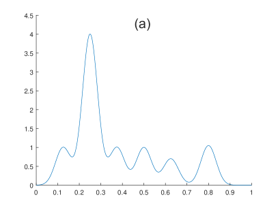
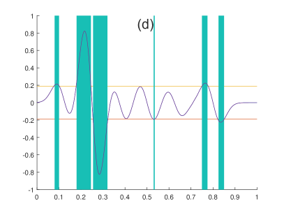
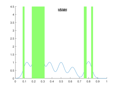
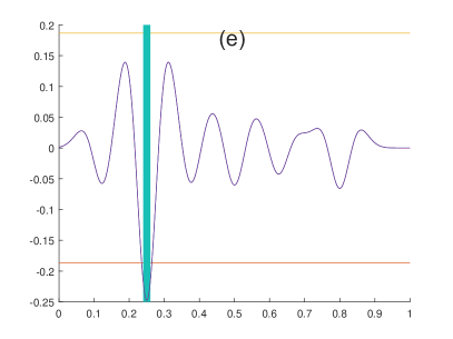
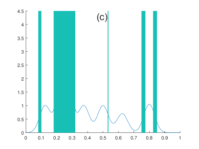
Figure 1: Relation between ${(A,B)}$-stability and ${{\mu}_{1:p}}$-stability for test function (figure (a)). Figure (b) shows ${(A,B)}$-stable regions (unshaded, $A=0.2$, $B=0.0125$). Figure (c) show ${{\mu}_{1:p}}$-stable regions (unshaded, ${\mu}={{\mu}^{-}}=0.1867$, derived from $A,B$ etc). Unstable maxima is $f(\frac{1}{4})=4$, stable maxima is $f(\frac{4}{5})=1.05$. Figures (d), (e) and (f) are first, second and third (scaled) gradients, respectively, where the shaded regions are ${{\mu}_{q}}$-unstable (so the shaded region in (c) is the combination (d) and (e)). Gradients above third order may be safely neglected here.

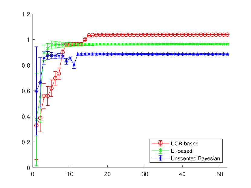
Figure 2: Convergence of the EISG, UCBSG and unscented acquisiton functions.

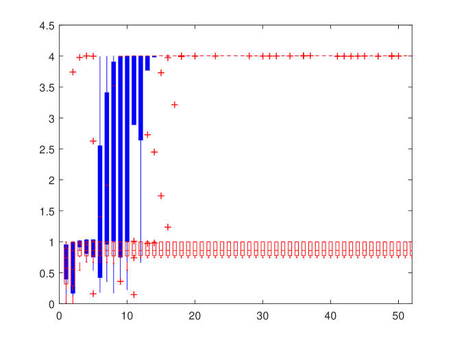
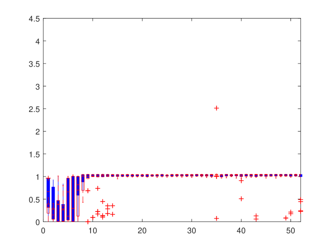
Figure 3: Recommendation box-plots for EISG (left) and UCBSG (right), with observations $f({\bf x}_{i})$ in blue and gains (calculated using post-simulation stability scores based on the complete set of observations) in red.

We have compared EISG (expected improvement in stable gain) and UCBSG (GP-UCB in stable gain) acquisition functions as well as unscented Bayesian optimisation and the stable Bayesian optimisation of [11, 10], with results shown in table 2. All experiments were repeated $10$ times. Note that neither unscented Bayesian optimisation nor [11, 10] are directly designed for this task and required some tweaking (in particular significantly increasing the variance of the input noise over that suggested by $B=0.0125$ to avoid always converging to the global maxima). Even after tweaking these algorithms still occasionally converged to the unstable maxima, so to ensure a fair comparison we have filtered out such cases.

The UCBSG acquisition function outperformed all other algorithms for this experiment. The reason for this is clear from figure 3, which shows $f({\bf x}_{t})$ and associated stable gains for recommendations over time. The EISG acquisition function tends to become “stuck” exploring the unstable global maxima, testing the same point over and over again. This provides no additional information for the gradient GP (and thus no additional information to update stability scores), as gradients are informed by the spread of samples around a point, so no additional information is gained and the process repeats. By contrast the explicit exploration term in the UCBSG acquisition function ensures a better spread of samples, so gradients (and thus stability scores) are correctly learnt and samples increasingly focus on the stable maxima.

7 Conclusions

In this paper we have studied the problem of finding stable maxima for expensive functions using a Gradient-based constraint as a surrogate for ${(A,B)}$-stability. We have also presented some theoretical analysis of the commection between ${(A,B)}$-stability and its surrogate to obtain bounds on the various parameters required. Our optimisation method is based on Bayesian optimisation. Using the novel concept of stable gain we have presented two acquisition function designed to avoid unstable regions in favour of stable solutions, namely expected improvement in stable gain (EISG) and GP upper confidence bound in stable gain (UCBSG), and experimentally we have compared these and also unscented Bayesian optimisation and stable Bayesian optimistion. Experimental results indicate that UCBSQ outperforms the alternative methods both in terms of reliability (likelihood that it will find a stable maxima) and convergence.

Appendix A Derivatives of Isotropic Kernels

Isotropic kernels [5] are kernels of the form:

$$\begin{array}[]{l}K\left({\bf x},{\bf x}^{\prime}\right)=\kappa\left(\frac{1}{2}\left\|{\bf x}-{\bf x}^{\prime}\right\|_{2}^{2}\right)\end{array}$$

Assume $K$ is $s$-times differentiable. In this section we consider the calculation of derivatives up to order $s$. Assuming that:

$$\begin{array}[]{l}\kappa^{(c)}\left(r\right)=\frac{\partial^{c}}{\partial r^{c}}\kappa\left(r\right)\;\forall c\in{\mathbb{Z}}_{s+1}\end{array}$$

can be calculated in closed form, we have the following results:

Theorem 1

Let $K({\bf x},{\bf x}^{\prime})=\kappa(\frac{1}{2}\|{\bf x}-{\bf x}^{\prime}\|_{2}^{2})$ be an isotropic kernel, where $\kappa$ is $s$-times differentiable. Denote by $\nabla_{{\bf x}^{\ldots}}^{\otimes q}$ a mixed Kronecker derivative of order $q$ (e.g. $\nabla_{{\bf x}^{\ldots}}^{\otimes 2}$ may be $\nabla_{{\bf x}}\otimes\nabla_{{\bf x}}$, $\nabla_{{\bf x}^{\prime}}\otimes\nabla_{{\bf x}^{\prime}}$, $\nabla_{{\bf x}}\otimes\nabla_{{\bf x}^{\prime}}$ or $\nabla_{{\bf x}^{\prime}}\otimes\nabla_{{\bf x}}$), where $\alpha$ is the number of times $\nabla_{{\bf x}^{\prime}}$ appears in $\nabla_{{\bf x}^{\ldots}}^{\otimes q}$. Then $\forall q\in{\mathbb{Z}}_{s+1}$:

$$\begin{array}[]{l}{\nabla_{{\bf x}^{\ldots}}^{\otimes q}K\left({\bf x},{\bf x}^{\prime}\right)=\left(-1\right)^{\alpha}\mathop{\sum}\limits_{i=0}^{\left\lfloor\frac{q}{2}\right\rfloor}{\bf a}_{(i,q)}\left({\bf x}^{\prime}-{\bf x}\right)\kappa^{(q-i)}\left(\frac{1}{2}\left\|{\bf x}-{\bf x}^{\prime}\right\|_{2}^{2}\right)}\end{array}$$

where $\kappa^{(c)}(x)=\frac{\partial^{c}}{\partial x^{c}}\kappa(x)$;

$$\begin{array}[]{rl}{\bf a}_{(i,q)}\left({\bf d}\right)&\!\!\!=\mathop{\sum}\limits_{{\bf j}\in{\mathbb{J}}_{(i,q)}}\;\;\mathop{\otimes}\limits_{k=0}^{q-1}\left\{\begin{array}[]{ll}\scriptstyle{{\bf x}^{\prime}-{\bf x}}&\scriptstyle{{\tt{if}}\;j_{k}=0}\\ \scriptstyle{{\mbox{\boldmath$\delta$}}_{j_{k}}}&\scriptstyle{\tt otherwise}\\ \end{array}\right.\end{array}$$ (15)

$$\begin{array}[]{l}\scriptstyle{{\mathbb{J}}_{(i,q)}=\{\left.{\bf j}\in{\mathbb{Z}}^{q}\right|\left\{j_{0},j_{1},\ldots,j_{q-1}\right\}=\left\{0,\ldots,0,-1,-1,-2,-2,\ldots,-i,-i\right\}\wedge\ldots}\\ \scriptstyle{\mathop{\operatorname{argmin}}\left\{\left.j_{k}\right|j_{k}=-1\right\}\leq\mathop{\operatorname{argmin}}\left\{\left.j_{k}\right|j_{k}=-2\right\}\leq\ldots\leq\mathop{\operatorname{argmin}}\left\{\left.j_{k}\right|j_{k}=-i\right\}\}}\end{array}$$

and we have used the symbolic notation (where ${\bf i}\in{\mathbb{Z}}_{n}^{q}$ is a multi-index, noting that ${\mbox{\boldmath$\delta$}}_{l}$’s appear in pairs in ${\bf a}_{(i,q)}$ $\forall l=-1,-2,\ldots,-i$):

$$\begin{array}[]{l}\scriptstyle{(\overbrace{\scriptstyle{\overset{\scriptscriptstyle{a\;{\tt{terms}}}}{\ldots}\otimes{\mbox{\boldmath$\delta$}}_{l}\otimes\ldots}}^{\scriptscriptstyle{b\;{\tt{terms}}}}\otimes{\mbox{\boldmath$\delta$}}_{l}\otimes\ldots)_{\bf i}=(\delta_{i_{a},i_{b}}(\overbrace{\scriptstyle{\overset{\scriptscriptstyle{a\;{\tt{terms}}}}{\ldots}\otimes{\bf 1}\otimes\ldots}}^{\scriptscriptstyle{b\;{\tt{terms}}}}\otimes{\bf 1}\otimes\ldots))_{\bf i}}\end{array}$$

Proof:

We begin by assuming $\alpha=0$. Defining ${\bf d}={\bf x}^{\prime}-{\bf x}$ we see that:

$$\begin{array}[]{rl}\scriptstyle{\nabla_{{\bf x}}^{\otimes 0}K\left({\bf x},{\bf x}^{\prime}\right)}&\!\!\!\!=\;\scriptstyle{\kappa^{(0)}\left(\frac{1}{2}\|{\bf x}^{\prime}-{\bf x}\|_{2}^{2}\right)}\\ \scriptstyle{\nabla_{{\bf x}}^{\otimes 1}K\left({\bf x},{\bf x}^{\prime}\right)}&\!\!\!\!=\;\scriptstyle{{\bf d}\kappa^{(1)}\left(\frac{1}{2}\|{\bf x}^{\prime}-{\bf x}\|_{2}^{2}\right)}\\ \scriptstyle{\nabla_{{\bf x}}^{\otimes 2}K\left({\bf x},{\bf x}^{\prime}\right)}&\!\!\!\!=\;\scriptstyle{\left({\bf d}\otimes{\bf d}\right)\kappa^{(2)}\left(\frac{1}{2}\|{\bf x}^{\prime}-{\bf x}\|_{2}^{2}\right)}\\ &\!\!\!\!+\;\scriptstyle{\left({\delta}_{-1}\otimes{\delta}_{-1}\right)\kappa^{(1)}\left(\frac{1}{2}\|{\bf x}^{\prime}-{\bf x}\|_{2}^{2}\right)}\\ \scriptstyle{\nabla_{{\bf x}}^{\otimes 3}K\left({\bf x},{\bf x}^{\prime}\right)}&\!\!\!\!=\;\scriptstyle{\left({\bf d}\otimes{\bf d}\otimes{\bf d}\right)\kappa^{(3)}\left(\frac{1}{2}\|{\bf x}^{\prime}-{\bf x}\|_{2}^{2}\right)}\\ &\!\!\!\!+\;\scriptstyle{\left({\bf d}\otimes{\delta}_{-1}\otimes{\delta}_{-1}+{\delta}_{-1}\otimes{\bf d}\otimes{\delta}_{-1}+{\delta}_{-1}\otimes{\delta}_{-1}\otimes{\bf d}\right)\kappa^{(2)}\left(\frac{1}{2}\|{\bf x}^{\prime}-{\bf x}\|_{2}^{2}\right)}\\ \scriptstyle{\nabla_{{\bf x}}^{\otimes 4}K\left({\bf x},{\bf x}^{\prime}\right)}&\!\!\!\!=\;\scriptstyle{\left({\bf d}\otimes{\bf d}\otimes{\bf d}\otimes{\bf d}\right)\kappa^{(4)}\left(\frac{1}{2}\|{\bf x}^{\prime}-{\bf x}\|_{2}^{2}\right)}\\ &\!\!\!\!\!\!\!\!\!\!\!\!\!\!\!\!\!\!\!\!\!\!\!\!\!\!\!\!\!\!\!\!\!\!\!\!\!\!\!\!\!\!\!\!\!\!\!\!\!\!+\scriptstyle{\left({\bf d}\otimes{\bf d}\otimes{\delta}_{-1}\otimes{\delta}_{-1}+{\bf d}\otimes{\delta}_{-1}\otimes{\bf d}\otimes{\delta}_{-1}+{\bf d}\otimes{\delta}_{-1}\otimes{\delta}_{-1}\otimes{\bf d}+{\delta}_{-1}\otimes{\bf d}\otimes{\bf d}\otimes{\delta}_{-1}+{\delta}_{-1}\otimes{\bf d}\otimes{\delta}_{-1}\otimes{\bf d}+{\delta}_{-1}\otimes{\delta}_{-1}\otimes{\bf d}\otimes{\bf d}\right)\kappa^{(3)}\left(\frac{1}{2}\|{\bf x}^{\prime}-{\bf x}\|_{2}^{2}\right)}\\ &\!\!\!\!+\;\scriptstyle{\left({\delta}_{-2}\otimes{\delta}_{-2}\otimes{\delta}_{-1}\otimes{\delta}_{-1}+{\delta}_{-2}\otimes{\delta}_{-1}\otimes{\delta}_{-2}\otimes{\delta}_{-1}+{\delta}_{-2}\otimes{\delta}_{-1}\otimes{\delta}_{-1}\otimes{\delta}_{-2}\right)\kappa^{(2)}\left(\frac{1}{2}\|{\bf x}^{\prime}-{\bf x}\|_{2}^{2}\right)}\\ \ldots\\ \end{array}$$

which confirms the first expression in the theorem for $q\leq 4$ when $\alpha=0$. More generally, suppose that for some $q>0$:

$$\begin{array}[]{rl}{\nabla_{{\bf x}}^{\otimes q}K\left({\bf x},{\bf x}^{\prime}\right)}&\!\!\!={\mathop{\sum}\limits_{i=0}^{\left\lfloor\frac{q}{2}\right\rfloor}{\bf a}_{(i,q)}\left({\bf x}^{\prime}-{\bf x}\right)\kappa^{(q-i)}\left(\frac{1}{2}\left\|{\bf x}-{\bf x}^{\prime}\right\|_{2}^{2}\right)}\\ &\!\!\!={\mathop{\sum}\limits_{i=0}^{\left\lfloor\frac{q}{2}\right\rfloor}\kappa^{(q-i)}\left(\frac{1}{2}\left\|{\bf x}-{\bf x}^{\prime}\right\|_{2}^{2}\right)}\mathop{\sum}\limits_{{\bf j}\in{\mathbb{J}}_{(i,q)}}\;\;\mathop{\otimes}\limits_{k=0}^{q-1}\left\{\begin{array}[]{ll}\scriptstyle{{\bf x}^{\prime}-{\bf x}}&\scriptstyle{{\tt{if}}\;j_{k}=0}\\ \scriptstyle{{\mbox{\boldmath$\delta$}}_{j_{k}}}&\scriptstyle{\tt otherwise}\\ \end{array}\right.\\ \end{array}$$

Then:

$$\begin{array}[]{rl}{\nabla_{{\bf x}}^{\otimes q+1}K\left({\bf x},{\bf x}^{\prime}\right)}&\!\!\!={\mathop{\sum}\limits_{i=0}^{\left\lfloor\frac{q}{2}\right\rfloor}\left(\nabla_{\bf x}\kappa^{(q-i)}\left(\frac{1}{2}\left\|{\bf x}-{\bf x}^{\prime}\right\|_{2}^{2}\right)\right)}\otimes\mathop{\sum}\limits_{{\bf j}\in{\mathbb{J}}_{(i,q)}}\;\;\mathop{\otimes}\limits_{k=0}^{q-1}\left\{\begin{array}[]{ll}\scriptstyle{{\bf x}^{\prime}-{\bf x}}&\scriptstyle{{\tt{if}}\;j_{k}=0}\\ \scriptstyle{{\mbox{\boldmath$\delta$}}_{j_{k}}}&\scriptstyle{\tt otherwise}\\ \end{array}\right.\\ &\!\!\!+{\mathop{\sum}\limits_{i=0}^{\left\lfloor\frac{q}{2}\right\rfloor}\kappa^{(q-i)}\left(\frac{1}{2}\left\|{\bf x}-{\bf x}^{\prime}\right\|_{2}^{2}\right)}\left(\mathop{\sum}\limits_{{\bf j}\in{\mathbb{J}}_{(i,q)}}\;\;\nabla_{\bf x}\otimes\mathop{\otimes}\limits_{k=0}^{q-1}\left\{\begin{array}[]{ll}\scriptstyle{{\bf x}^{\prime}-{\bf x}}&\scriptstyle{{\tt{if}}\;j_{k}=0}\\ \scriptstyle{{\mbox{\boldmath$\delta$}}_{j_{k}}}&\scriptstyle{\tt otherwise}\\ \end{array}\right.\right)\\ &\!\!\!={\mathop{\sum}\limits_{i=0}^{\left\lfloor\frac{q}{2}\right\rfloor}\left(\kappa^{(q-i+1)}\left(\frac{1}{2}\left\|{\bf x}-{\bf x}^{\prime}\right\|_{2}^{2}\right)\right)}\left({\bf x}^{\prime}-{\bf x}\right)\otimes\mathop{\sum}\limits_{{\bf j}\in{\mathbb{J}}_{(i,q)}}\;\;\mathop{\otimes}\limits_{k=0}^{q-1}\left\{\begin{array}[]{ll}\scriptstyle{{\bf x}^{\prime}-{\bf x}}&\scriptstyle{{\tt{if}}\;j_{k}=0}\\ \scriptstyle{{\mbox{\boldmath$\delta$}}_{j_{k}}}&\scriptstyle{\tt otherwise}\\ \end{array}\right.\\ &\!\!\!+{\mathop{\sum}\limits_{i=0}^{\left\lfloor\frac{q}{2}\right\rfloor}\kappa^{(q-i)}\left(\frac{1}{2}\left\|{\bf x}-{\bf x}^{\prime}\right\|_{2}^{2}\right)}\left(\mathop{\sum}\limits_{{\bf j}\in{\mathbb{J}}_{(i,q)}}\mathop{\sum}\limits_{l:j_{l}=0}{\mbox{\boldmath$\delta$}}_{-(i+1)}\otimes\mathop{\otimes}\limits_{k=0}^{q-1}\left\{\begin{array}[]{ll}\scriptstyle{{\bf x}^{\prime}-{\bf x}}&\scriptstyle{{\tt{if}}\;j_{k}=0\wedge k\neq l}\\ \scriptstyle{{\mbox{\boldmath$\delta$}}_{-(i+1)}}&\scriptstyle{\tt{if}}\;j_{k}=0\wedge k=l\\ \scriptstyle{{\mbox{\boldmath$\delta$}}_{j_{k}}}&\scriptstyle{\tt otherwise}\\ \end{array}\right.\right)\\ \end{array}$$

and it follows by index rearrangement that:

$$\begin{array}[]{rl}{\nabla_{{\bf x}}^{\otimes q+1}K\left({\bf x},{\bf x}^{\prime}\right)}&\!\!\!={\mathop{\sum}\limits_{i=0}^{\left\lfloor\frac{q+1}{2}\right\rfloor}{\bf a}_{(i,q+1)}\left({\bf x}^{\prime}-{\bf x}\right)\kappa^{(q+1-i)}\left(\frac{1}{2}\left\|{\bf x}-{\bf x}^{\prime}\right\|_{2}^{2}\right)}\\ \end{array}$$

Therefore by induction $\forall q\in{\mathbb{Z}}_{+}$:

$$\begin{array}[]{rl}{\nabla_{{\bf x}}^{\otimes q}K\left({\bf x},{\bf x}^{\prime}\right)}&\!\!\!={\mathop{\sum}\limits_{i=0}^{\left\lfloor\frac{q}{2}\right\rfloor}{\bf a}_{(i,q)}\left({\bf x}^{\prime}-{\bf x}\right)\kappa^{(q-i)}\left(\frac{1}{2}\left\|{\bf x}-{\bf x}^{\prime}\right\|_{2}^{2}\right)}\\ \end{array}$$

The final result ($\alpha\geq 0$) follows by observing the sign-anti-symmetry of ${\bf x}$ and ${\bf x}^{\prime}$ in all expressions. $\square$

Appendix B Proof of Theorems 2 and 3

In this section we prove theorems 1 and 2 from the body of the paper. Before proceeding with this we first establish some preliminary results. Finally, we consider some examples of kernels and derive the relevant constants relating to the theorems. Throughout this section we use the shorthand:

$$\begin{array}[]{l}f^{(i)}\left(x\right)=\frac{\partial^{i}}{\partial x^{i}}f\left(x\right)\end{array}$$

We will also be using the Hermite polynomials $H_{q}$ and the normalised Hermite polynomials (Hermite functions) $h_{q}$ [1]:

$$\begin{array}[]{rl}H_{q}\left(x\right)&\!\!\!=\mathop{\sum}\limits_{i=0}^{\left\lfloor\frac{q}{2}\right\rfloor}\left(-1\right)^{i}n_{(i,q)}x^{q-2i}\\ h_{q}\left(x\right)&\!\!\!=\frac{1}{\sqrt{2^{q}q!\sqrt{\pi}}}e^{-\frac{1}{2}x^{2}}\mathop{\sum}\limits_{i=0}^{\left\lfloor\frac{q}{2}\right\rfloor}\left(-1\right)^{i}n_{(i,q)}x^{q-2i}\\ \end{array}$$ (16)

where:

$$\begin{array}[]{l}n_{(i,q)}=\frac{q!}{2^{i}i!(q-2i)!}\end{array}$$

As per the paper, it is assumed throughout that:

1. ${\mathbb{X}}\subset{\mathbb{R}}^{n}$ compact, $\|{\bf x}-{\bf x}^{\prime}\|_{2}\leq M$ $\forall{\bf x},{\bf x}^{\prime}\in{\mathbb{X}}$.

2. $f:{\mathbb{X}}\subseteq{\mathbb{R}}^{n}\to{\mathbb{R}}_{+}\sim\operatorname{{\mathcal{GP}}}(0,K({\bf x},{\bf x}^{\prime}))$.

3. $\|f\|_{{\mathbb{H}}_{K}}\leq G$, where $\|\cdot\|_{{\mathbb{H}}_{K}}$ is the reproducing kernel Hilbert space norm.

4. $K({\bf x},{\bf x}^{\prime})=\kappa(\frac{1}{2}\|{\bf x}-{\bf x}^{\prime}\|_{2}^{2})$ is isotropic kernel (covariance), $\kappa$ is completely monotone, positive, $s$-times differentiable, and there exist $L^{\uparrow}\geq L^{\downarrow}\in{\mathbb{R}}_{+}$, $\Delta_{r}:{\mathbb{R}}_{+}\to{\mathbb{R}}_{+}$ non-decreasing such that:

   $$\begin{array}[]{l}L^{\downarrow q}\kappa\left(r\right)\leq\left|\kappa^{(q)}\left(r\right)\right|\leq L^{\uparrow q}\kappa\left(r\right)\;\forall q\in{\mathbb{Z}}_{s+1}\\ \left|\kappa\left(r+\delta r\right)-\mathop{\sum}\limits_{q\in{\mathbb{Z}}_{s+1}}\frac{1}{q!}\delta r^{q}\kappa^{(q)}\left(r\right)\right|\leq\Delta_{r}\left(\delta r\right)\end{array}$$

   and we define the overall Taylor bound for $\kappa$ as:

   $$\begin{array}[]{l}\Delta\left(\delta r\right)=\mathop{\sup}\limits_{r\in\left[0,\frac{1}{2}M^{2}\right)}\frac{\Delta_{r}\left(\delta r\right)}{\kappa\left(r\right)}\end{array}$$

B.1 Preliminary Results

The following preliminary results are required:

Theorem I

The number of terms in the sum ${\bf a}_{(i,q)}$ as defined by (15) is:

$$\begin{array}[]{l}n_{(i,q)}=\frac{q!}{2^{i}i!(q-2i)!}\end{array}$$

which are the same terms that occur in the Hermite polynomial (LABEL:eq:hermpoly).

Proof:

We aim to count the number of distinct vectors ${\bf j}\in{\mathbb{Z}}^{q}$ such that $\{j_{0},j_{1},\ldots,j_{q-1}\}=\{0,0,\ldots,0,-1,-1,-2,-2,\ldots,-i,-i\}$ and $\operatorname{argmin}\{j_{k}:j_{k}=-1\}\leq\operatorname{argmin}\{j_{k}:j_{k}=-2\}\leq\ldots\leq\operatorname{argmin}\{j_{k}:j_{k}=-i\}$.

Ignoring constraints, there are $q!$ permutations $(j_{0},j_{1},\ldots,j_{q-1})$ such that $\{j_{0},j_{1},\ldots,j_{q-1}\}=\{0,0,\ldots,0,-1,-1,-2,-2,\ldots,-i,-i\}$. Of these, $(q-2i)!$ are redundant reshuffles of $0$ elements, $2$ are redundant reshuffles of $-1$ elements, $2$ are redundant reshuffles of $-2$ elements, $\ldots$, and $2$ are redundant reshuffles of $-i$ elements. Thus there are $\frac{q!}{2^{i}(q-2i)!}$ distinct vectors ${\bf j}$ such that $\{j_{0},j_{1},\ldots,j_{q-1}\}=\{0,0,\ldots,0,-1,-1,-2,-2,\ldots,-i,-i\}$. Note that only $1$ out of every $i!$ of these vectors satisfies the condition $\operatorname{argmin}\{j_{k}:j_{k}=-1\}\leq\operatorname{argmin}\{j_{k}:j_{k}=-2\}\leq\ldots\leq\operatorname{argmin}\{j_{k}:j_{k}=-i\}$, leaving a total of $n_{(i,q)}$ terms in the sum (each corresponding to a vector ${\bf j}$).

The final result follows from the definition of the Hermite polynomials ([1], table 22.3). $\square$

Theorem II

Under the default assumptions:

$$\begin{array}[]{l}{\frac{1}{q!}\left|\delta{\bf x}^{\otimes q{\rm T}}{\nabla_{{\bf x}}^{\otimes q}K\left({\bf x},{\bf x}^{\prime}\right)}\right|\leq\sqrt{\frac{2^{q}}{q!}}\left(D^{\uparrow}+\frac{1}{\sqrt{2^{q}}}D_{(q)}^{\updownarrow}\right)\left(\sqrt{L^{\uparrow}}\left\|\delta{\bf x}\right\|_{2}\right)^{q}\kappa\left(\frac{1}{2}\left\|{\bf x}-{\bf x}^{\prime}\right\|_{2}^{2}\right)}\\ \end{array}$$

$\forall q\in{\mathbb{Z}}_{s+1}$, where:

$$\begin{array}[]{rl}D^{\uparrow}&\!\!\!=0.816\pi^{\frac{1}{4}}e^{\frac{1}{2}\left(\sqrt{L^{\uparrow}}M\right)^{2}}\\ D_{(q)}^{\updownarrow}&\!\!\!=\frac{L^{\uparrow}-L^{\downarrow}}{L^{\uparrow}}\mathop{\sum}\limits_{i=0}^{\left\lfloor\frac{1}{2}\left\lfloor\frac{q}{2}\right\rfloor\right\rfloor}\frac{\sqrt{q!}}{2^{2i}(2i)!(q-4i)!}\left(\sqrt{L^{\uparrow}-L^{\downarrow}}M\right)^{q-4i}\\ \end{array}$$

where $D_{(q)}^{\updownarrow}=0$ if $L^{\uparrow}=L^{\downarrow}$.

Proof:

Recall the definition of ${\bf a}_{(i,q)}$ in theorem 1 and $n_{(i,q)}$ from theorem I. Using multi-index notation we see that:

$$\begin{array}[]{rl}\delta{\bf x}^{\otimes q{\rm T}}{\bf a}_{(i,q)}\left({\bf x}\right)&\!\!\!=\left|\mathop{\sum}\limits_{{\bf j}\in{\mathbb{Z}}_{n}^{q}}\delta{\bf x}_{j_{0}}\delta{\bf x}_{j_{1}}\ldots\delta{\bf x}_{j_{q-1}}{\bf a}_{(i,q){\bf j}}\left({\bf x}\right)\right|\\ &\!\!\!=n_{(i,q)}\left\|\delta{\bf x}\right\|_{2}^{2i}\left({\bf x}^{{\rm T}}\delta{\bf x}\right)^{q-2i}\\ \end{array}$$

and so:

$$\begin{array}[]{rl}\left|\delta{\bf x}^{\otimes q{\rm T}}{\nabla_{{\bf x}}^{\otimes q}K\left({\bf x},{\bf x}^{\prime}\right)}\right|&\!\!\!=\left|\mathop{\sum}\limits_{i=0}^{\left\lfloor\frac{q}{2}\right\rfloor}\delta{\bf x}^{\otimes q{\rm T}}{\bf a}_{(i,q)}\left({\bf x}^{\prime}-{\bf x}\right)\kappa^{(q-i)}\left(\frac{1}{2}\left\|{\bf x}-{\bf x}^{\prime}\right\|_{2}^{2}\right)\right|\\ &\!\!\!=\left|\mathop{\sum}\limits_{i=0}^{\left\lfloor\frac{q}{2}\right\rfloor}n_{(i,q)}\left\|\delta{\bf x}\right\|_{2}^{2i}\left(\left({\bf x}-{\bf x}^{\prime}\right)^{{\rm T}}\delta{\bf x}\right)^{q-2i}\kappa^{(q-i)}\left(\frac{1}{2}\left\|{\bf x}-{\bf x}^{\prime}\right\|_{2}^{2}\right)\right|\\ \end{array}$$

By assumption 4 it follows that, defining $L^{\updownarrow}=L^{\uparrow}-L^{\downarrow}$ and letting $L_{[i]}\in[L^{\uparrow},L^{\downarrow}]$ $\forall i\in{\mathbb{Z}}_{q+1}$ such that the first statement in the following is true (this is always possible by the definition of $L^{\uparrow}$, $L^{\downarrow}$ in assumption 4 and the complete monotonicity of $\kappa$):

$$\begin{array}[]{rl}\scriptstyle{\left|\delta{\bf x}^{\otimes q{\rm T}}{\nabla_{{\bf x}}^{\otimes q}K\left({\bf x},{\bf x}^{\prime}\right)}\right|}&\!\!\!\scriptstyle{=\left|\mathop{\sum}\limits_{i=0}^{\left\lfloor\frac{q}{2}\right\rfloor}n_{(i,q)}\left\|\delta{\bf x}\right\|_{2}^{2i}\left(\left({\bf x}-{\bf x}^{\prime}\right)^{{\rm T}}\delta{\bf x}\right)^{q-2i}L_{[q-i]}^{q-i}\left(-1\right)^{q-i}\kappa\left(\frac{1}{2}\left\|{\bf x}-{\bf x}^{\prime}\right\|_{2}^{2}\right)\right|}\\ &\!\!\!\scriptstyle{=\left|\mathop{\sum}\limits_{i=0}^{\left\lfloor\frac{q}{2}\right\rfloor}n_{(i,q)}\left\|\delta{\bf x}\right\|_{2}^{q}\left|\left({\bf x}-{\bf x}^{\prime}\right)^{{\rm T}}\frac{\delta{\bf x}}{\left\|\delta{\bf x}\right\|_{2}}\right|^{q-2i}L_{[q-i]}^{q-i}\left(-1\right)^{i}\kappa\left(\frac{1}{2}\left\|{\bf x}-{\bf x}^{\prime}\right\|_{2}^{2}\right)\right|}\\ &\!\!\!\scriptstyle{\leq\left|\mathop{\sum}\limits_{i=0}^{\left\lfloor\frac{q}{2}\right\rfloor}n_{(i,q)}\left\|\delta{\bf x}\right\|_{2}^{q}\left|\left({\bf x}-{\bf x}^{\prime}\right)^{{\rm T}}\frac{\delta{\bf x}}{\left\|\delta{\bf x}\right\|_{2}}\right|^{q-2i}L^{\uparrow q-i}\left(-1\right)^{i}\kappa\left(\frac{1}{2}\left\|{\bf x}-{\bf x}^{\prime}\right\|_{2}^{2}\right)\right|}\\ &\!\!\!\scriptstyle{+\left|\mathop{\sum}\limits_{{i=0}\atop{i\;{\rm odd}}}^{\left\lfloor\frac{q}{2}\right\rfloor}n_{(i,q)}\left\|\delta{\bf x}\right\|_{2}^{q}\left|\left({\bf x}-{\bf x}^{\prime}\right)^{{\rm T}}\frac{\delta{\bf x}}{\left\|\delta{\bf x}\right\|_{2}}\right|^{q-2i}L^{\updownarrow q-i}\kappa\left(\frac{1}{2}\left\|{\bf x}-{\bf x}^{\prime}\right\|_{2}^{2}\right)\right|}\\ &\!\!\!\scriptstyle{=\left(\sqrt{L^{\uparrow}}\left\|\delta{\bf x}\right\|_{2}\right)^{q}\left|\mathop{\sum}\limits_{i=0}^{\left\lfloor\frac{q}{2}\right\rfloor}\left(-1\right)^{i}n_{(i,q)}\left|\sqrt{L^{\uparrow}}\left({\bf x}-{\bf x}^{\prime}\right)^{{\rm T}}\frac{\delta{\bf x}}{\left\|\delta{\bf x}\right\|_{2}}\right|^{q-2i}\right|\kappa\left(\frac{1}{2}\left\|{\bf x}-{\bf x}^{\prime}\right\|_{2}^{2}\right)}\\ &\!\!\!\scriptstyle{+\left(\sqrt{L^{\updownarrow}}\left\|\delta{\bf x}\right\|_{2}\right)^{q}\left(\mathop{\sum}\limits_{{i=0}\atop{i\;{\rm odd}}}^{\left\lfloor\frac{q}{2}\right\rfloor}n_{(i,q)}\left|\sqrt{L^{\updownarrow}}\left({\bf x}-{\bf x}^{\prime}\right)^{{\rm T}}\frac{\delta{\bf x}}{\left\|\delta{\bf x}\right\|_{2}}\right|^{q-2i}\right)\kappa\left(\frac{1}{2}\left\|{\bf x}-{\bf x}^{\prime}\right\|_{2}^{2}\right)}\\ \end{array}$$

So, by the definition of the normalised Hermite polynomial (LABEL:eq:hermpoly):

$$\begin{array}[]{rl}\scriptstyle{\left|\delta{\bf x}^{\otimes q{\rm T}}{\nabla_{{\bf x}}^{\otimes q}K\left({\bf x},{\bf x}^{\prime}\right)}\right|}&\!\!\!\scriptstyle{\leq\left(\sqrt{L^{\uparrow}}\left\|\delta{\bf x}\right\|_{2}\right)^{q}\sqrt{2^{q}q!\sqrt{\pi}}e^{\frac{1}{2}\left|\sqrt{L^{\uparrow}}\left({\bf x}-{\bf x}^{\prime}\right)^{{\rm T}}\frac{\delta{\bf x}}{\left\|\delta{\bf x}\right\|_{2}}\right|^{2}}\left|h_{q}\left(\left|\sqrt{L^{\uparrow}}\left({\bf x}-{\bf x}^{\prime}\right)^{{\rm T}}\frac{\delta{\bf x}}{\left\|\delta{\bf x}\right\|_{2}}\right|\right)\right|\kappa\left(\frac{1}{2}\left\|{\bf x}-{\bf x}^{\prime}\right\|_{2}^{2}\right)}\\ &\!\!\!\scriptstyle{+\left(\sqrt{L^{\updownarrow}}\left\|\delta{\bf x}\right\|_{2}\right)^{q}\left(\mathop{\sum}\limits_{{i=0}\atop{i\;{\rm odd}}}^{\left\lfloor\frac{q}{2}\right\rfloor}n_{(i,q)}\left|\sqrt{L^{\updownarrow}}\left({\bf x}-{\bf x}^{\prime}\right)^{{\rm T}}\frac{\delta{\bf x}}{\left\|\delta{\bf x}\right\|_{2}}\right|^{q-2i}\right)\kappa\left(\frac{1}{2}\left\|{\bf x}-{\bf x}^{\prime}\right\|_{2}^{2}\right)}\\ &\!\!\!\scriptstyle{\leq\left(\sqrt{L^{\uparrow}}\left\|\delta{\bf x}\right\|_{2}\right)^{q}\sqrt{2^{q}q!\sqrt{\pi}}e^{\frac{1}{2}\left(\sqrt{L^{\uparrow}}\left\|{\bf x}-{\bf x}^{\prime}\right\|_{2}\right)^{2}}\left|h_{q}\left(\left|\sqrt{L^{\uparrow}}\left({\bf x}-{\bf x}^{\prime}\right)^{{\rm T}}\frac{\delta{\bf x}}{\left\|\delta{\bf x}\right\|_{2}}\right|\right)\right|\kappa\left(\frac{1}{2}\left\|{\bf x}-{\bf x}^{\prime}\right\|_{2}^{2}\right)}\\ &\!\!\!\scriptstyle{+\left(\sqrt{L^{\updownarrow}}\left\|\delta{\bf x}\right\|_{2}\right)^{q}\left(\mathop{\sum}\limits_{{i=0}\atop{i\;{\rm odd}}}^{\left\lfloor\frac{q}{2}\right\rfloor}n_{(i,q)}\left(\sqrt{L^{\updownarrow}}\left\|{\bf x}-{\bf x}^{\prime}\right\|_{2}\right)^{q-2i}\right)\kappa\left(\frac{1}{2}\left\|{\bf x}-{\bf x}^{\prime}\right\|_{2}^{2}\right)}\\ \end{array}$$

Note from [1, 2] that $|h_{q}(x)|<0.816$, so:

$$\begin{array}[]{l}\begin{array}[]{rl}\scriptstyle{\left|\delta{\bf x}^{\otimes q{\rm T}}{\nabla_{{\bf x}}^{\otimes q}K\left({\bf x},{\bf x}^{\prime}\right)}\right|}&\!\!\!\scriptstyle{\leq\Big{(}0.816\left(\sqrt{L^{\uparrow}}\left\|\delta{\bf x}\right\|_{2}\right)^{q}\sqrt{2^{q}q!\sqrt{\pi}}e^{\frac{1}{2}\left(\sqrt{L^{\uparrow}}\left\|{\bf x}-{\bf x}^{\prime}\right\|_{2}\right)^{2}}}\\ &\!\!\!\scriptstyle{+\left(\sqrt{L^{\updownarrow}}\left\|\delta{\bf x}\right\|_{2}\right)^{q}\mathop{\sum}\limits_{{i=0}\atop{i\;{\rm odd}}}^{\left\lfloor\frac{q}{2}\right\rfloor}n_{(i,q)}\left(\sqrt{L^{\updownarrow}}\left\|{\bf x}-{\bf x}^{\prime}\right\|_{2}\right)^{q-2i}\Big{)}\kappa\left(\frac{1}{2}\left\|{\bf x}-{\bf x}^{\prime}\right\|_{2}^{2}\right)}\\ \end{array}\\ \scriptstyle{=\sqrt{2^{q}q!}\Big{(}\left(\sqrt{L^{\uparrow}}\left\|\delta{\bf x}\right\|_{2}\right)^{q}0.816\pi^{\frac{1}{4}}e^{\frac{1}{2}\left(\sqrt{L^{\uparrow}}\left\|{\bf x}-{\bf x}^{\prime}\right\|_{2}\right)^{2}}+\frac{1}{\sqrt{2^{q}}}\left(\sqrt{L^{\updownarrow}}\left\|\delta{\bf x}\right\|_{2}\right)^{q}\tilde{h}_{q}\left(\sqrt{L^{\updownarrow}}\left\|{\bf x}-{\bf x}^{\prime}\right\|_{2}\right)\Big{)}\kappa\left(\frac{1}{2}\left\|{\bf x}-{\bf x}^{\prime}\right\|_{2}^{2}\right)}\\ \end{array}$$

where:

$$\begin{array}[]{l}\tilde{h}_{q}\left(t\right)=\mathop{\sum}\limits_{i=0}^{\left\lfloor\frac{1}{2}\left\lfloor\frac{q}{2}\right\rfloor\right\rfloor}\frac{\sqrt{q!}}{2^{2i}(2i)!(q-4i)!}t^{q-4i}\end{array}$$

is non-decreasing for $t\in{\mathbb{R}}_{+}$, so by the assumed bounds:

$$\begin{array}[]{l}\scriptstyle{\frac{1}{q!}\left|\delta{\bf x}^{\otimes q{\rm T}}{\nabla_{{\bf x}}^{\otimes q}K\left({\bf x},{\bf x}^{\prime}\right)}\right|\leq\sqrt{\frac{2^{q}}{q!}}\Big{(}\left(\sqrt{L^{\uparrow}}\left\|\delta{\bf x}\right\|_{2}\right)^{q}0.816\pi^{\frac{1}{4}}e^{\frac{1}{2}\left(\sqrt{L^{\uparrow}}M\right)^{2}}+\frac{1}{\sqrt{2^{q}}}\left(\sqrt{L^{\updownarrow}}\left\|\delta{\bf x}\right\|_{2}\right)^{q}\tilde{h}_{q}\left(\sqrt{L^{\updownarrow}}M\right)\Big{)}\kappa\left(\frac{1}{2}\left\|{\bf x}-{\bf x}^{\prime}\right\|_{2}^{2}\right)}\\ \end{array}$$

or, re-writing:

$$\begin{array}[]{l}\scriptstyle{\frac{2^{q}}{q!}\left|\delta{\bf x}^{\otimes q{\rm T}}{\nabla_{{\bf x}}^{\otimes q}K\left({\bf x},{\bf x}^{\prime}\right)}\right|\leq\sqrt{\frac{1}{q!}}\left(\sqrt{L^{\uparrow}}\left\|\delta{\bf x}\right\|_{2}\right)^{q}\left(0.816\pi^{\frac{1}{4}}e^{\frac{1}{2}\left(\sqrt{L^{\uparrow}}M\right)^{2}}+\frac{1}{\sqrt{2^{q}}}\left(\frac{L^{\uparrow}-L^{\downarrow}}{L^{\uparrow}}\right)^{\frac{q}{2}}\tilde{h}_{q}\left(\sqrt{L^{\uparrow}-L^{\downarrow}}M\right)\right)\kappa\left(\frac{1}{2}\left\|{\bf x}-{\bf x}^{\prime}\right\|_{2}^{2}\right)}\\ \end{array}$$

Finally, noting that $\frac{L^{\uparrow}-L^{\downarrow}}{L^{\uparrow}}\in[0,1]$, it follows that:

$$\begin{array}[]{l}\scriptstyle{\frac{1}{q!}\left|\delta{\bf x}^{\otimes q{\rm T}}{\nabla_{{\bf x}}^{\otimes q}K\left({\bf x},{\bf x}^{\prime}\right)}\right|\leq\sqrt{\frac{2^{q}}{q!}}\left(\sqrt{L^{\uparrow}}\left\|\delta{\bf x}\right\|_{2}\right)^{q}\left(0.816\pi^{\frac{1}{4}}e^{\frac{1}{2}\left(\sqrt{L^{\uparrow}}M\right)^{2}}+\frac{1}{\sqrt{2^{q}}}\frac{L^{\uparrow}-L^{\downarrow}}{L^{\uparrow}}\tilde{h}_{q}\left(\sqrt{L^{\uparrow}-L^{\downarrow}}M\right)\right)\kappa\left(\frac{1}{2}\left\|{\bf x}-{\bf x}^{\prime}\right\|_{2}^{2}\right)}\\ \end{array}$$

and the result follows. $\square$

Theorem III

Under the default assumptions, the remainders of $\kappa({\bf x}+\delta{\bf x})$ Taylor expanded around ${\bf x}\in{\mathbb{X}}$, to order $p\in{\mathbb{Z}}_{s+1}$ are bounded by:

$$\begin{array}[]{l}\scriptstyle{\left|\mathop{\sum}\limits_{q=p+1}^{s}\frac{1}{q!}\delta{\bf x}^{\otimes q}{}^{\rm T}\nabla_{\bf x}^{\otimes q}\kappa\left({\bf x}\right)\right|\leq\left(\left(D^{\uparrow}+D^{\updownarrow}\right)\sqrt{\frac{1}{(p+1)!}}\frac{\left(\sqrt{2L^{\uparrow}}B\right)^{p+1}-\left(\sqrt{2L^{\uparrow}}B\right)^{s+1}}{1-\left(\sqrt{2L^{\uparrow}}B\right)}+\frac{\Delta_{\frac{1}{2}\left\|{\bf x}\right\|_{2}^{2}}\left(\frac{1}{2}B^{2}\right)}{\left|\kappa\left(\frac{1}{2}\left\|{\bf x}\right\|_{2}^{2}\right)\right|}\right)\kappa\left(\frac{1}{2}\left\|{\bf x}\right\|_{2}^{2}\right)}\end{array}$$

$\forall\delta{\bf x}:\|\delta{\bf x}\|_{2}\leq B<\frac{1}{\sqrt{2L^{\uparrow}}}$, where:

$$\begin{array}[]{rl}D^{\uparrow}&\!\!\!=0.816\pi^{\frac{1}{4}}e^{\frac{1}{2}\left(\sqrt{L^{\uparrow}}M\right)^{2}}\\ D^{\updownarrow}&\!\!\!=\frac{L^{\uparrow}-L^{\downarrow}}{L^{\uparrow}}\mathop{\sum}\limits_{i=0}^{s}\mathop{\sum}\limits_{i=0}^{\left\lfloor\frac{1}{2}\left\lfloor\frac{q}{2}\right\rfloor\right\rfloor}\frac{\sqrt{q!}}{2^{2i}(2i)!(q-4i)!}\left(\sqrt{L^{\uparrow}-L^{\downarrow}}M\right)^{q-4i}\\ \end{array}$$

where $D^{\updownarrow}=0$ if $L^{\uparrow}=L^{\downarrow}$.

Proof:

Taylor expanding to order $p\in{\mathbb{Z}}_{s+1}$:

$$\begin{array}[]{rl}\kappa\left(\frac{1}{2}\left\|{\bf x}+\delta{\bf x}\right\|_{2}^{2}\right)&\!\!\!=\mathop{\sum}\limits_{q\in{\mathbb{Z}}_{p+1}}\frac{1}{q!}\delta{\bf x}^{\otimes q}{}^{\rm T}\nabla_{\bf x}^{\otimes q}\kappa\left(\frac{1}{2}\left\|{\bf x}\right\|_{2}^{2}\right)+r_{p:{\bf x}}\left(\delta{\bf x}\right)\\ \end{array}$$

and so:

$$\begin{array}[]{rl}\left|r_{p:{\bf x}}\left(\delta{\bf x}\right)\right|&\!\!\!\leq\left|\mathop{\sum}\limits_{q=p+1}^{s}\frac{1}{q!}\delta{\bf x}^{\otimes q}{}^{\rm T}\nabla_{\bf x}^{\otimes q}\kappa\left(\frac{1}{2}\left\|{\bf x}\right\|_{2}^{2}\right)\right|+\Delta_{\frac{1}{2}\left\|{\bf x}\right\|_{2}^{2}}\left(\frac{1}{2}\left\|\delta{\bf x}\right\|_{2}^{2}\right)\end{array}$$

Using theorem II we see that:

$$\begin{array}[]{l}\scriptstyle{\left|\mathop{\sum}\limits_{q=p+1}^{s}\frac{1}{q!}\delta{\bf x}^{\otimes q}{}^{\rm T}\nabla_{\bf x}^{\otimes q}\kappa\left({\bf x}\right)\right|\leq\left|\mathop{\sum}\limits_{q=p+1}^{s}\sqrt{\frac{2^{q}}{q!}}\left(D^{\uparrow}+\frac{1}{\sqrt{2^{q}}}D^{\updownarrow}_{q}\right)\left(\sqrt{L^{\uparrow}}\left\|\delta{\bf x}\right\|_{2}\right)^{q}\right|\kappa\left(\frac{1}{2}\left\|{\bf x}\right\|_{2}^{2}\right)}\\ \;\;\;\scriptstyle{\leq\left(\left|D^{\uparrow}\mathop{\sum}\limits_{q=p+1}^{s}\sqrt{\frac{1}{q!}}\left(\sqrt{2L^{\uparrow}}\left\|\delta{\bf x}\right\|_{2}\right)^{q}\right|+\left|\mathop{\sum}\limits_{q=p+1}^{s}\sqrt{\frac{1}{2^{q}q!}}D^{\updownarrow}_{q}\left(\sqrt{2L^{\uparrow}}\left\|\delta{\bf x}\right\|_{2}\right)^{q}\right|\right)\kappa\left(\frac{1}{2}\left\|{\bf x}\right\|_{2}^{2}\right)}\\ \;\;\;\scriptstyle{\leq\left(\left|D^{\uparrow}\sqrt{\frac{1}{(p+1)!}}\mathop{\sum}\limits_{q=p+1}^{s}\left(\sqrt{2L^{\uparrow}}\left\|\delta{\bf x}\right\|_{2}\right)^{q}\right|+\left|\sqrt{\frac{1}{(p+1)!}}\mathop{\sum}\limits_{q=p+1}^{s}D^{\updownarrow}_{q}\left(\sqrt{2L^{\uparrow}}\left\|\delta{\bf x}\right\|_{2}\right)^{q}\right|\right)\kappa\left(\frac{1}{2}\left\|{\bf x}\right\|_{2}^{2}\right)}\\ \;\;\;\scriptstyle{\leq\left(\left|D^{\uparrow}\sqrt{\frac{1}{(p+1)!}}\mathop{\sum}\limits_{q=p+1}^{s}\left(\sqrt{2L^{\uparrow}}\left\|\delta{\bf x}\right\|_{2}\right)^{q}\right|+\left|\sqrt{\frac{1}{(p+1)!}}\left(\mathop{\sum}\limits_{q=p+1}^{s}D^{\updownarrow}_{q}\right)\left(\mathop{\sum}\limits_{q=p+1}^{s}\left(\sqrt{2L^{\uparrow}}\left\|\delta{\bf x}\right\|_{2}\right)^{q}\right)\right|\right)\kappa\left(\frac{1}{2}\left\|{\bf x}\right\|_{2}^{2}\right)}\\ \;\;\;\scriptstyle{\leq\sqrt{\frac{1}{(p+1)!}}D_{p}\mathop{\sum}\limits_{q=p+1}^{s}\left(\sqrt{2L^{\uparrow}}B\right)^{q}\kappa\left(\frac{1}{2}\left\|{\bf x}\right\|_{2}^{2}\right)}\\ \end{array}$$

where:

$$\begin{array}[]{rl}D_{p}&\!\!\!=0.816\pi^{\frac{1}{4}}e^{\frac{1}{2}\left(\sqrt{L^{\uparrow}}M\right)^{2}}+\frac{L^{\uparrow}-L^{\downarrow}}{L^{\uparrow}}\mathop{\sum}\limits_{q=p+1}^{s}\mathop{\sum}\limits_{i=0}^{\left\lfloor\frac{1}{2}\left\lfloor\frac{q}{2}\right\rfloor\right\rfloor}\frac{\sqrt{q!}}{2^{2i}(2i)!(q-4i)!}\left(\sqrt{L^{\uparrow}-L^{\downarrow}}M\right)^{q-4i}\\ \end{array}$$

is non-increasing with $p$. Moreover:

$$\begin{array}[]{l}\mathop{\sum}\limits_{q=p+1}^{s}\left(\sqrt{2L^{\uparrow}}B\right)^{q}=\frac{\left(\sqrt{2L^{\uparrow}}B\right)^{p+1}-\left(\sqrt{2L^{\uparrow}}B\right)^{s+1}}{1-\left(\sqrt{2L^{\uparrow}}B\right)}\end{array}$$

which is well-defined by assumption $\sqrt{2L^{\uparrow}}B<1$. Therefore:

$$\begin{array}[]{l}\scriptstyle{\left|\mathop{\sum}\limits_{q=p+1}^{s}\frac{1}{q!}\delta{\bf x}^{\otimes q}{}^{\rm T}\nabla_{\bf x}^{\otimes q}\kappa\left({\bf x}\right)\right|\leq\sqrt{\frac{1}{(p+1)!}}D_{0}\frac{\left(\sqrt{2L^{\uparrow}}B\right)^{p+1}-\left(\sqrt{2L^{\uparrow}}B\right)^{s+1}}{1-\left(\sqrt{2L^{\uparrow}}B\right)}\kappa\left(\frac{1}{2}\left\|{\bf x}\right\|_{2}^{2}\right)}\end{array}$$

and the result follows, noting that $\Delta_{r}$ is non-decreasing. $\square$

B.2 Main Proofs

Theorem 2

Let $A,B\in{\mathbb{R}}_{+}$, $s\in{\mathbb{Z}}_{+}$. Under the default assumptions, suppose the remainders of $f({\bf x}+\delta{\bf x})$ Taylor expanded about ${\bf x}\in{\mathbb{X}}$ to order $q$ satisfy the bound $|R_{q:{\bf x}}(\delta{\bf x})|\leq U_{q}(B)$ $\forall\delta{\bf x},\|\delta{\bf x}\|_{2}\leq B$. Define:

$$\begin{array}[]{l}{\mathbb{P}}=\left\{p\in{\mathbb{Z}}_{s}+1\left|U_{p}\left(B\right)\leq A\right.\right\}\\ \end{array}$$

If ${\mathbb{P}}\neq\emptyset$, $p\in{\mathbb{P}}$, and ${{{\mu}^{\pm}}}=(A\pm U_{p}(B))$ then, using ${{\mu}^{+}_{1:p}}$-stability and ${{\mu}^{-}_{1:p}}$-stability to denote ${{\mu}_{1:p}}$-stability with, respectively, ${\mu}={{\mu}^{+}}$ and ${\mu}={{\mu}^{-}}$, we have:

$$\begin{array}[]{l}{\mathbb{S}}_{{{\mu}^{-}_{1:p}}}\subseteq{\mathbb{S}}_{{(A,B)}}\subseteq{\mathbb{S}}_{{{\mu}^{+}_{1:p}}}\end{array}$$

Proof:

Suppose ${\bf x}\in{\mathbb{S}}_{{(A,B)}}$. As $f$ is $s$-times differentiable and ${(A,B)}$-stable at ${\bf x}$, and using the fact that $({\bf a}\otimes{\bf b})^{{\rm T}}({\bf c}\otimes{\bf d})=({\bf a}^{{\rm T}}{\bf c})({\bf b}^{{\rm T}}{\bf d})$:

$$\begin{array}[]{rl}A&\!\!\!\geq\left|f\left({\bf x}\right)-f\left({\bf x}+\delta{\bf x}\right)\right|\\ &\!\!\!=\left|\sum_{r\in{\mathbb{Z}}_{p}+1}\frac{1}{r!}\delta{\bf x}^{\otimes r}{}^{\rm T}\nabla_{\bf x}^{\otimes r}f\left({\bf x}\right)+R_{p:{\bf x}}\left(\delta{\bf x}\right)\right|\\ &\!\!\!\geq\left|\sum_{r\in{\mathbb{Z}}_{p}+1}\frac{1}{r!}\delta{\bf x}^{\otimes r}{}^{\rm T}\nabla_{\bf x}^{\otimes r}f\left({\bf x}\right)\right|-\left|R_{p:{\bf x}}\left(\delta{\bf x}\right)\right|\\ &\!\!\!\geq\left|\frac{1}{q!}\delta{\bf x}^{\otimes q}{}^{\rm T}\nabla_{\bf x}^{\otimes q}f\left({\bf x}\right)\right|-\left|R_{p:{\bf x}}\left(\delta{\bf x}\right)\right|\\ \end{array}$$

$\forall q\in{\mathbb{Z}}_{p}+1$, $\delta{\bf x}:\|\delta{\bf x}\|_{2}\leq B$. Hence:

$$\begin{array}[]{rl}\mathop{\sup}\limits_{\delta{\bf x}:\left\|\delta{\bf x}\right\|_{2}=B}\left|\frac{1}{q!}\delta{\bf x}^{\otimes q}{}^{\rm T}\nabla_{\bf x}^{\otimes q}f\left({\bf x}\right)\right|&\!\!\!=\frac{1}{q!}\left\|\nabla_{\bf x}^{\otimes q}f\left({\bf x}\right)\right\|_{2}\left\|\delta{\bf x}\right\|_{2}^{q}=\frac{B^{q}}{q!}\left\|\nabla_{\bf x}^{\otimes q}f\left({\bf x}\right)\right\|_{2}\\ \end{array}$$

Substituting, we find that, under the conditions of the theorem $\forall q\in{\mathbb{Z}}_{p}+1$:

$$\begin{array}[]{rl}\left\|\frac{B^{q}}{q!}\nabla_{\bf x}^{\otimes q}f\left({\bf x}\right)\right\|_{2}&\!\!\!\leq\left(A+U_{p}\left(B\right)\right)\end{array}$$

and hence ${\bf x}\in{\mathbb{S}}_{{{\mu}^{+}_{1:p}}}$, ${\mathbb{S}}_{{(A,B)}}\subseteq{\mathbb{S}}_{{{\mu}^{+}_{1:p}}}$.

Next suppose ${\bf x}\in{\mathbb{S}}_{{{\mu}^{-}_{1:p}}}$. As $f$ is $s$-times differentiable:

$$\begin{array}[]{rl}\left|f\left({\bf x}\right)-f\left({\bf x}+\delta{\bf x}\right)\right|&\!\!\!=\left|\sum_{q\in{\mathbb{Z}}_{p}+1}\frac{1}{q!}\delta{\bf x}^{\otimes q}{}^{\rm T}\nabla_{\bf x}^{\otimes q}f\left({\bf x}\right)+R_{p:{\bf x}}\left(\delta{\bf x}\right)\right|\\ &\!\!\!\leq\sum_{q\in{\mathbb{Z}}_{p}+1}\frac{1}{q!}\left|\delta{\bf x}^{\otimes q}{}^{\rm T}\nabla_{\bf x}^{\otimes q}f\left({\bf x}\right)\right|+\left|R_{p:{\bf x}}\left(\delta{\bf x}\right)\right|\\ &\!\!\!\leq\sum_{q\in{\mathbb{Z}}_{p}+1}\frac{1}{q!}\left\|\delta{\bf x}^{\otimes q}\right\|_{2}\left\|\nabla_{\bf x}^{\otimes q}f\left({\bf x}\right)\right\|_{2}+\left|R_{p:{\bf x}}\left(\delta{\bf x}\right)\right|\\ &\!\!\!\leq{{\mu}^{-}}\sum_{q\in{\mathbb{Z}}_{p}+1}B^{-q}\left\|\delta{\bf x}\right\|_{2}^{q}+\left|R_{p:{\bf x}}\left(\delta{\bf x}\right)\right|\\ \end{array}$$

$\forall q\in{\mathbb{Z}}_{p}+1$. We want to show that this implies ${\bf x}\in{\mathbb{S}}_{{(A,B)}}$ or, equivalently, that $|f({\bf x})-f({\bf x}+\delta{\bf x})|\leq A$ $\forall\delta{\bf x}:\|\delta{\bf x}\|_{2}\leq B$. It suffices to show that for $p$, ${{\mu}^{-}}$ specified, $\forall\delta{\bf x}:\|\delta{\bf x}\|_{2}\leq B$:

$$\begin{array}[]{rl}{{\mu}^{-}}\sum_{q\in{\mathbb{Z}}_{p}+1}B^{-q}\left\|\delta{\bf x}\right\|_{2}^{q}+\left|R_{p:{\bf x}}\left(\delta{\bf x}\right)\right|\leq A\end{array}$$

or, equivalently, that for $p$, ${{\mu}^{-}}$ specified, ${{\mu}^{-}}\leq A-U_{p}\left(B\right)>0$, which is true by definition of ${{\mu}^{-}}$ and $p$ in the theorem. $\square$

Theorem 3

Under the default assumptions $|f({\bf x})|<F$, where:

$$\begin{array}[]{l}F=\kappa\left(0\right)\sqrt{\frac{\pi^{\frac{1}{2}n}}{\Gamma\left(\frac{1}{2}n+1\right)}\left(\frac{M}{2}\right)^{n}}G\end{array}$$

and the remainders of $f({\bf x}+\delta{\bf x})$ Taylor expanded around ${\bf x}\in{\mathbb{X}}$ to order $q\in{\mathbb{Z}}_{s}+1$ are bounded by:

$$\begin{array}[]{r}\left|R_{q:{\bf x}}\left(\delta{\bf x}\right)\right|\leq\left(\left(D^{\uparrow}+D^{\updownarrow}\right)\frac{1}{\sqrt{(q+1)!}}\frac{\left(\sqrt{2L^{\uparrow}}B\right)^{q+1}-\left(\sqrt{2L^{\uparrow}}B\right)^{s+1}}{1-\sqrt{2L^{\uparrow}}B}+\Delta\left(\frac{1}{2}B^{2}\right)\right)F\end{array}$$

$\forall\delta{\bf x}:\|\delta{\bf x}\|_{2}\leq B<\frac{1}{\sqrt{2L^{\uparrow}}}$, where:

$$\begin{array}[]{rl}D^{\uparrow}&\!\!\!=0.816\pi^{\frac{1}{4}}e^{\frac{1}{2}\left(\sqrt{L^{\uparrow}}M\right)^{2}}\\ D^{\updownarrow}&\!\!\!=\frac{L^{\uparrow}-L^{\downarrow}}{L^{\uparrow}}\mathop{\sum}\limits_{i=0}^{s}\mathop{\sum}\limits_{i=0}^{\left\lfloor\frac{1}{2}\left\lfloor\frac{q}{2}\right\rfloor\right\rfloor}\frac{\sqrt{q!}}{2^{2i}(2i)!(q-4i)!}\left(\sqrt{L^{\uparrow}-L^{\downarrow}}M\right)^{q-4i}\\ \end{array}$$

noting that $D^{\updownarrow}=0$ if $L^{\uparrow}=L^{\downarrow}$. If $\Delta(\frac{1}{2}B^{2})F<A$ then $|R_{p:{\bf x}}(\delta{\bf x})|\leq A$ $\forall p\geq p_{\rm min}$, where:

$$\begin{array}[]{l}\scriptscriptstyle{p_{\rm min}=\max\left\{1,\left\lceil\left(\sqrt{2L^{\uparrow}}B\right)^{2}\exp\left(1+W_{0}\left(\frac{2}{e\left(\sqrt{2L^{\uparrow}}B\right)^{2}}\log\left(\frac{1}{\sqrt{\sqrt{2\pi}}}\frac{\left(D^{\uparrow}+D^{\updownarrow}\right)F}{A-\Delta(\frac{1}{2}B^{2})F}\frac{1}{1-\sqrt{2L^{\uparrow}}B}\right)\right)\right)-1\right\rceil\right\}}\\ \end{array}$$

where $W_{0}$ is the principle branch of the Lambert $W$-function.

Proof:

We have that ${\mathbb{X}}$ is compact and finite dimensional with maximum (Euclidean) distance between points in ${\mathbb{X}}$ being $M$. The maximum hypervolume of ${\mathbb{X}}$ satisfying these criteria is that of an $|{\mathbb{X}}|$-ball with diameter $M$ - that is, the Lebesgue measure of ${\mathbb{X}}$ is bounded as:

$$\begin{array}[]{l}\mu\left({\mathbb{X}}\right)\leq\frac{\pi^{\frac{1}{2}n}}{\Gamma\left(\frac{1}{2}n+1\right)}\left(\frac{M}{2}\right)^{n}\end{array}$$

We have that $f\in{\mathbb{H}}_{K}$, where ${\mathbb{H}}_{K}$ is the reproducing kernel Hilbert space associated with $K$, as $f$ is a draw from an unbiased Gaussian process with zero mean and kernel $K$. Hence $\exists\alpha\in L_{2}({\mathbb{X}})$ such that:

$$\begin{array}[]{rl}f\left({\bf x}\right)&\!\!\!=\mathop{\int}\limits_{\tilde{\bf x}\in{\mathbb{X}}}\alpha\left(\tilde{\bf x}\right)K\left({\bf x},\tilde{\bf x}\right)d\tilde{\bf x}\\ &\!\!\!=\mathop{\int}\limits_{\tilde{\bf x}\in{\mathbb{X}}}\alpha\left(\tilde{\bf x}\right)\kappa\left(\frac{1}{2}\left\|{\bf x}-\tilde{\bf x}\right\|_{2}^{2}\right)d\tilde{\bf x}\\ \end{array}$$

where $\|f\|_{{\mathbb{H}}_{K}}=\|\alpha\|_{L_{2}({\mathbb{X}})}$ (as $f\in{\mathbb{H}}_{K}$ there exist at least one $\alpha\in L_{2}({\mathbb{X}})$ such that $f$ has the above form, and by definition $\|f\|_{{\mathbb{H}}_{K}}=\inf_{\alpha}\|\alpha\|_{H}$, so we choose the minimum norm $\alpha$). Using standard properties of $L_{p}$-norms, we also have that:

$$\begin{array}[]{rl}\left\|\alpha\right\|_{L_{1}\left({\mathbb{X}}\right)}&\!\!\!\leq\sqrt{\mu\left({\mathbb{X}}\right)}\left\|\alpha\right\|_{L_{2}\left({\mathbb{X}}\right)}\\ &\!\!\!\leq\sqrt{\frac{\pi^{\frac{1}{2}n}}{\Gamma\left(\frac{1}{2}n+1\right)}\left(\frac{M}{2}\right)^{n}}\left\|\alpha\right\|_{L_{2}\left({\mathbb{X}}\right)}\\ &\!\!\!=\sqrt{\frac{\pi^{\frac{1}{2}n}}{\Gamma\left(\frac{1}{2}n+1\right)}\left(\frac{M}{2}\right)^{n}}\left\|f\right\|_{{\mathbb{H}}_{K}}\\ \end{array}$$

Moreover, using Hölder’s inequality and the positivity and complete monotonicity of $\kappa$:

$$\begin{array}[]{rl}\left|f\left({\bf x}\right)\right|&\!\!\!=\left|\mathop{\int}\limits_{\tilde{\bf x}\in{\mathbb{X}}}\alpha\left(\tilde{\bf x}\right)\kappa\left({\bf x}-\tilde{\bf x}\right)d\tilde{\bf x}\right|\\ &\!\!\!\leq\left\|\alpha\right\|_{L_{1}\left({\mathbb{X}}\right)}\mathop{\max}\limits_{\tilde{\bf x}\in{\mathbb{X}}}\left\{\kappa\left(\frac{1}{2}\left\|{\bf x}-\tilde{\bf x}\right\|_{2}^{2}\right)\right\}\\ &\!\!\!\leq\sqrt{\frac{\pi^{\frac{1}{2}n}}{\Gamma\left(\frac{1}{2}n+1\right)}\left(\frac{M}{2}\right)^{n}}\kappa\left(0\right)\left\|\alpha\right\|_{L_{2}({\mathbb{X}})}\\ &\!\!\!=\sqrt{\frac{\pi^{\frac{1}{2}n}}{\Gamma\left(\frac{1}{2}n+1\right)}\left(\frac{M}{2}\right)^{n}}\kappa\left(0\right)\left\|f\right\|_{{\mathbb{H}}_{K}}=F\\ \end{array}$$

Next, let $p\in{\mathbb{Z}}_{s+1}$. We know that:

$$\begin{array}[]{rl}f\left({\bf x}+\delta{\bf x}\right)&\!\!\!=\mathop{\int}\limits_{\tilde{\bf x}\in{\mathbb{X}}}\alpha\left(\tilde{\bf x}\right)\kappa\left(\frac{1}{2}\left\|\left({\bf x}-\tilde{\bf x}\right)+\delta{\bf x}\right\|_{2}^{2}\right)d\tilde{\bf x}\\ \end{array}$$

and the Taylor expansion of $f$ to order $p$ about ${\bf x}$ is:

$$\begin{array}[]{rl}f\left({\bf x}+\delta{\bf x}\right)&\!\!\!=\mathop{\sum}\limits_{q\in{\mathbb{Z}}_{p+1}}\frac{1}{q!}\delta{\bf x}^{\otimes q{\rm T}}\nabla_{\bf x}^{\otimes q}f\left({\bf x}\right)+R_{p:{\bf x}}\left(\delta{\bf x}\right)\\ &\!\!\!=\mathop{\int}\limits_{\tilde{\bf x}\in{\mathbb{X}}}\alpha\left(\tilde{\bf x}\right)\mathop{\sum}\limits_{q\in{\mathbb{Z}}_{p+1}}\frac{1}{q!}\delta{\bf x}^{\otimes q{\rm T}}\nabla_{\bf x}^{\otimes q}\kappa\left(\frac{1}{2}\left\|{\bf x}-\tilde{\bf x}\right\|_{2}^{2}\right)d\tilde{\bf x}+R_{p:{\bf x}}\left(\delta{\bf x}\right)\\ \end{array}$$

where $R_{p:{\bf x}}(\delta{\bf x})$ is the remainder; and hence:

$$\begin{array}[]{rl}R_{p:{\bf x}}\left(\delta{\bf x}\right)=\mathop{\int}\limits_{\tilde{\bf x}\in{\mathbb{X}}}\alpha\left(\tilde{\bf x}\right)r_{p:{\bf x}-\tilde{\bf x}}\left(\delta{\bf x}\right)d\tilde{\bf x}\end{array}$$

where:

$$\begin{array}[]{rl}\kappa\left(\frac{1}{2}\left\|{\bf x}+\delta{\bf x}\right\|_{2}^{2}\right)&\!\!\!=\mathop{\sum}\limits_{q\in{\mathbb{Z}}_{p+1}}\frac{1}{q!}\delta{\bf x}^{\otimes q{\rm T}}\nabla_{\bf x}^{\otimes q}\kappa\left(\frac{1}{2}\left\|{\bf x}\right\|_{2}^{2}\right)+r_{p:{\bf x}}\left(\delta{\bf x}\right)\\ \end{array}$$

Defining $S_{p:\delta{\bf x}}({\bf x})=R_{p:{\bf x}}(\delta{\bf x})$, we see that:

$$\begin{array}[]{rl}S_{p:\delta{\bf x}}\left({\bf x}\right)&\!\!\!=\mathop{\int}\limits_{\tilde{\bf x}\in{\mathbb{X}}}\alpha\left(\tilde{\bf x}\right)r_{p:{\bf x}-\tilde{\bf x}}\left(\delta{\bf x}\right)d\tilde{\bf x}\\ &\!\!\!=\mathop{\int}\limits_{\tilde{\bf x}\in{\mathbb{X}}}\left(\frac{r_{p:{\bf x}-\tilde{\bf x}}\left(\delta{\bf x}\right)}{\kappa\left(\frac{1}{2}\left\|{\bf x}-\tilde{\bf x}\right\|_{2}^{2}\right)}\right)\alpha\left(\tilde{\bf x}\right)\kappa\left(\frac{1}{2}\left\|{\bf x}-\tilde{\bf x}\right\|_{2}^{2}\right)d{\bf x}\\ \end{array}$$

and hence, by Hölder’s inequality:

$$\begin{array}[]{rl}\left\|S_{p:\delta{\bf x}}\left({\bf x}\right)\right\|_{L_{1}({\mathbb{X}})}&\!\!\!\leq\mathop{\sup}\limits_{\tilde{\bf x}\in{\mathbb{X}}}\left|\left(\frac{r_{p:{\bf x}-\tilde{\bf x}}\left(\delta{\bf x}\right)}{\kappa\left(\frac{1}{2}\left\|{\bf x}-\tilde{\bf x}\right\|_{2}^{2}\right)}\right)\right|\mathop{\sup}\limits_{\tilde{\bf x}\in{\mathbb{X}}}\left|\kappa\left(\frac{1}{2}\left\|{\bf x}-\tilde{\bf x}\right\|_{2}^{2}\right)\right|\left\|\alpha\right\|_{L_{1}({\mathbb{X}})}\\ &\!\!\!\leq\mathop{\sup}\limits_{\tilde{\bf x}\in{\mathbb{X}}}\left|\left(\frac{r_{p:{\bf x}-\tilde{\bf x}}\left(\delta{\bf x}\right)}{\kappa\left(\frac{1}{2}\left\|{\bf x}-\tilde{\bf x}\right\|_{2}^{2}\right)}\right)\right|\kappa\left(0\right)\sqrt{\frac{\pi^{\frac{1}{2}n}}{\Gamma\left(\frac{1}{2}n+1\right)}\left(\frac{M}{2}\right)^{n}}\left\|\alpha\right\|_{L_{2}({\mathbb{X}})}\\ &\!\!\!=\mathop{\sup}\limits_{\tilde{\bf x}\in{\mathbb{X}}}\left|\left(\frac{r_{p:{\bf x}-\tilde{\bf x}}\left(\delta{\bf x}\right)}{\kappa\left(\frac{1}{2}\left\|{\bf x}-\tilde{\bf x}\right\|_{2}^{2}\right)}\right)\right|\kappa\left(0\right)\sqrt{\frac{\pi^{\frac{1}{2}n}}{\Gamma\left(\frac{1}{2}n+1\right)}\left(\frac{M}{2}\right)^{n}}\left\|f\right\|_{{\mathbb{H}}_{K}}\\ &\!\!\!=\mathop{\sup}\limits_{\tilde{\bf x}\in{\mathbb{X}}}\left|\left(\frac{r_{p:{\bf x}-\tilde{\bf x}}\left(\delta{\bf x}\right)}{\kappa\left(\frac{1}{2}\left\|{\bf x}-\tilde{\bf x}\right\|_{2}^{2}\right)}\right)\right|F\\ \end{array}$$

Recall from theorem III that, defining $D=D^{\uparrow}+D^{\updownarrow}$:

$$\begin{array}[]{rl}\left|\frac{r_{p:{\bf x}}\left(\delta{\bf x}\right)}{\kappa\left(\frac{1}{2}\left\|{\bf x}\right\|_{2}^{2}\right)}\right|&\!\!\!\leq D\sqrt{\frac{1}{(p+1)!}}\frac{\left(\sqrt{2L^{\uparrow}}B\right)^{p+1}-\left(\sqrt{2L^{\uparrow}}B\right)^{s+1}}{1-\left(\sqrt{2L^{\uparrow}}B\right)}+\frac{\Delta_{\frac{1}{2}\left\|{\bf x}\right\|_{2}^{2}}\left(\frac{1}{2}B^{2}\right)}{\kappa\left(\frac{1}{2}\left\|{\bf x}\right\|_{2}^{2}\right)}\\ &\!\!\!\leq D\sqrt{\frac{1}{(p+1)!}}\frac{\left(\sqrt{2L^{\uparrow}}B\right)^{p+1}-\left(\sqrt{2L^{\uparrow}}B\right)^{s+1}}{1-\left(\sqrt{2L^{\uparrow}}B\right)}+\Delta\left(\frac{1}{2}B^{2}\right)\\ \end{array}$$

and hence:

$$\begin{array}[]{l}\left|R_{p:{\bf x}}\left(\delta{\bf x}\right)\right|=\left|S_{p:\delta{\bf x}}\left({\bf x}\right)\right|\leq\left\|S_{p:\delta{\bf x}}\left({\bf x}\right)\right\|_{L_{1}({\mathbb{X}})}\leq\left(D\sqrt{\frac{1}{(p+1)!}}\frac{\left(\sqrt{2L^{\uparrow}}B\right)^{p+1}-\left(\sqrt{2L^{\uparrow}}B\right)^{s+1}}{1-\left(\sqrt{2L^{\uparrow}}B\right)}+\Delta\left(\frac{1}{2}B^{2}\right)\right)F\\ \end{array}$$

Finally we must prove the bound $p\geq p_{\rm min}$ so that $|R_{p:{\bf x}}(\delta{\bf x})|\leq A$ $\forall\delta{\bf x}$ satisfying relevant bounds. First we note that, trivially:

$$\begin{array}[]{rl}\left|R_{p:{\bf x}}\left(\delta{\bf x}\right)\right|&\!\!\!\leq\left(D\sqrt{\frac{1}{(p+1)!}}\frac{\left(\sqrt{2L^{\uparrow}}B\right)^{p+1}}{1-\left(\sqrt{2L^{\uparrow}}B\right)}+\Delta\left(\frac{1}{2}M^{2}\right)\right)F\end{array}$$

Hence it suffices that $p_{\rm min}$ satisfies:

$$\begin{array}[]{l}(p_{\rm min}+1)!\geq\left(\frac{DF}{A-\Delta(\frac{1}{2}M^{2})F}\right)^{2}\left(\frac{\left(\sqrt{2L^{\uparrow}}B\right)^{p_{\rm min}+1}}{1-\sqrt{2L^{\uparrow}}B}\right)^{2}\\ \end{array}$$

By Stirling’s approximation we know that [16]:

$$\begin{array}[]{l}(p+1)!>\sqrt{2\pi(p+1)}\left(\frac{p+1}{e}\right)^{p+1}>\sqrt{2\pi}\left(\frac{p+1}{e}\right)^{p+1}\end{array}$$

so it suffices to find $p_{\rm min}$ such that:

$$\begin{array}[]{l}\sqrt{2\pi}\left(\frac{p_{\rm min}+1}{e}\right)^{p_{\rm min}+1}\geq\left(\frac{DF}{A-\Delta(\frac{1}{2}M^{2})F}\right)^{2}\left(\frac{\left(\sqrt{2L^{\uparrow}}B\right)^{p_{\rm min}+1}}{1-\sqrt{2L^{\uparrow}}B}\right)^{2}\\ \end{array}$$

or, equivalently, taking the natural log both sides and simplifying:

$$\begin{array}[]{l}\scriptscriptstyle{\frac{p_{\rm min}+1}{e\left(\sqrt{2L^{\uparrow}}B\right)^{2}}\log\left(\frac{p_{\rm min}+1}{e\left(\sqrt{2L^{\uparrow}}B\right)^{2}}\right)\geq\frac{2}{e\left(\sqrt{2L^{\uparrow}}B\right)^{2}}\log\left(\frac{1}{\sqrt{\sqrt{2\pi}}}\frac{DF}{A-\Delta(\frac{1}{2}M^{2})F}\frac{1}{1-\sqrt{2L^{\uparrow}}B}\right)}\\ \end{array}$$

Let $y=\frac{p_{\rm min}+1}{e(\sqrt{2L^{\uparrow}}\|\delta{\bf x}\|_{2})^{2}}$. Then the preceding equation reduces to finding $y$ such that:

$$\begin{array}[]{l}y\log\left(y\right)\geq\frac{2}{e\left(\sqrt{2L^{\uparrow}}B\right)^{2}}\log\left(\frac{1}{\sqrt{\sqrt{2\pi}}}\frac{DF}{A-\Delta(\frac{1}{2}M^{2})F}\frac{1}{1-\sqrt{2L^{\uparrow}}B}\right)\\ \end{array}$$

which is simply the inverse of the Lambert $W$-function (principle branch). Hence it suffices that:

$$\begin{array}[]{l}{\log\left(y\right)\geq W_{0}\left(\frac{2}{e\left(\sqrt{2L^{\uparrow}}B\right)^{2}}\log\left(\frac{1}{\sqrt{\sqrt{2\pi}}}\frac{DF}{A-\Delta(\frac{1}{2}M^{2})F}\frac{1}{1-\sqrt{2L^{\uparrow}}B}\right)\right)}\\ \end{array}$$

That is:

$$\begin{array}[]{l}\scriptscriptstyle{p_{\rm min}=\max\left\{1,\left\lceil\left(\sqrt{2L^{\uparrow}}B\right)^{2}\exp\left(1+W_{0}\left(\frac{2}{e\left(\sqrt{2L^{\uparrow}}B\right)^{2}}\log\left(\frac{1}{\sqrt{\sqrt{2\pi}}}\frac{DF}{A-\Delta(\frac{1}{2}M^{2})F}\frac{1}{1-\sqrt{2L^{\uparrow}}B}\right)\right)\right)-1\right\rceil\right\}}\\ \end{array}$$

which completes the proof. $\square$

Appendix C Properties of Standard Isotropic Kernel

In this section we consider the two kernels that are appropriate for our method and one counter-example to illustrate the limitations.

C.1 RBF Kernel

The RBF kernel is defined by:

$$\begin{array}[]{l}K\left({\bf x},{\bf x}^{\prime}\right)=\kappa_{(\gamma)}\left(\frac{1}{2}\left\|{\bf x}-{\bf x}^{\prime}\right\|_{2}^{2}\right)\\ \kappa_{(\gamma)}\left(r\right)=e^{-\frac{1}{\gamma^{2}}r}\end{array}$$

where $\gamma\in{\mathbb{R}}_{+}$. We see immediately that $\kappa$ is infinitely differentiable, where:

$$\begin{array}[]{rl}\kappa_{(\gamma)}^{(q)}\left(r\right)=\left(-\frac{1}{\gamma^{2}}\right)^{q}\kappa_{(\gamma)}\left(r\right)\\ \end{array}$$

It follows trivially that:

$$\begin{array}[]{l}L_{(\gamma)}^{\downarrow q}\kappa_{(\gamma)}\left(r\right)\leq\left|\kappa_{(\gamma)}^{(q)}\left(r\right)\right|\leq L_{(\gamma)}^{\uparrow q}\kappa_{(\gamma)}\left(r\right)\\ \end{array}$$

where:

$$\begin{array}[]{l}L_{(\gamma)}^{\uparrow}=L_{(\gamma)}^{\downarrow}=\frac{1}{\gamma^{2}}\end{array}$$

Note also that the Taylor expansion of the RBF kernel is convergent, so:

$$\begin{array}[]{l}\Delta_{(\gamma)r}\left(\delta r\right)=\Delta_{(\gamma)}\left(\delta r\right)=0\end{array}$$

C.2 Matérn Kernels

The Matérn kernel is defined by:

$$\begin{array}[]{l}K\left({\bf x},{\bf x}^{\prime}\right)=\kappa_{(\nu,\rho)}\left(\frac{1}{2}\left\|{\bf x}-{\bf x}^{\prime}\right\|_{2}^{2}\right)\\ \kappa_{(\nu,\rho)}\left(r\right)=\frac{2^{1-\nu}}{\Gamma\left(\nu\right)}\left(\sqrt{2\nu}\frac{1}{\rho}\sqrt{2r}\right)^{\nu}{\rm H}_{\nu}\left(\sqrt{2\nu}\frac{1}{\rho}\sqrt{2r}\right)\end{array}$$

where $\nu,\rho\in{\mathbb{R}}_{+}$ and ${\rm H}_{\nu}$ is a modified Bessel function of the second kind. From [1] ((9.6.28) with trivial rearrangement) we have that:

$$\begin{array}[]{l}\left(\frac{1}{z}\frac{\partial}{\partial z}\right)^{q}\left(\frac{2^{1-\nu}}{\Gamma\left(\nu\right)}z^{\nu}H_{\nu}\left(z\right)\right)=\left(\left(-\frac{1}{2}\right)^{q}\frac{\Gamma\left(\nu-q\right)}{\Gamma\left(\nu\right)}\right)\frac{2^{1-(\nu-q)}}{\Gamma\left(\nu-q\right)}z^{\nu-q}H_{\nu-q}\left(z\right)\end{array}$$

and hence $\forall q\in{\mathbb{Z}}_{\lceil\nu\rceil}$:

$$\begin{array}[]{l}\kappa_{(\nu,\rho)}^{(q)}\left(r\right)=\left(\left(-\frac{\sqrt{\nu}}{2\rho}\right)^{q}\frac{\Gamma\left(\nu-q\right)}{\Gamma\left(\nu\right)}\right)\kappa_{(\nu-q,\rho)}\left(r\right)\end{array}$$ (17)

Note that, while this indicates that derivatives do exist to arbitrary order for $\nu\in{\mathbb{R}}_{+}\backslash{\mathbb{Z}}$ as ${\rm H}_{-\nu}={\rm H}_{\nu}$ (the gamma function has poles at $\nu=0,-1,-2,\ldots$, so the derivative is ill-defined if $\nu\in{\mathbb{Z}}_{+}$ and $q\geq\nu$), the result only defines a kernel for $q\leq{\lceil\nu\rceil-1}$. Thus the derivatives of a Gaussian process with a Matérn kernel are only Gaussian processes to order $q\leq{\lceil\nu\rceil-1}$. Of equal importance here, the derivatives of order $q>{\lceil\nu\rceil-1}$ have a pole at $r=0$, so the Taylor series approximation will construct in our proofs will diverge when constructed to order $p>{\lceil\nu\rceil-1}$. So in effect, for practical purposes, we say that $K$ is $\lceil\nu\rceil-1$ times differentiable. Of particular interest are the cases:

$$\begin{array}[]{rl}\kappa_{(d+\frac{1}{2},\rho)}\left(r\right)&\!\!\!=\exp\left(-\sqrt{2d+1}\frac{1}{\rho}\sqrt{2r}\right)\frac{d!}{(2d)!}\mathop{\sum}\limits_{i\in{\mathbb{Z}}_{d+1}}\frac{(d+i)!}{i!(d-i)!}\left(2\sqrt{2d+1}\frac{1}{\rho}\sqrt{2r}\right)^{d-i}\\ \kappa_{(\infty,\rho)}\left(r\right)&\!\!\!=\exp\left(-\frac{1}{\rho^{2}}r\right)\\ \end{array}$$

where $d\in{\mathbb{Z}}_{\infty}$, where the latter is simply the RBF kernel.

We postulate the following:

Postulate IV

For all $d\in{\mathbb{Z}}_{\infty}$ the ratio function:

$$\begin{array}[]{l}R_{d}\left(r\right)=\frac{\kappa_{(d+\frac{1}{2},\rho)}\left(r\right)}{\kappa_{(d+\frac{3}{2},\rho)}\left(r\right)}\end{array}$$

has only three stationary points - one local maxima $R_{d}\left(0\right)=1$ and two local minima $R_{d}\left(\pm\tilde{r}_{d}\right)<1$ - and in the limits $\mathop{\lim}\limits_{r\to\pm\infty}R_{d}\left(r\right)=\infty$. Furthermore, defining $\beta_{d}=\mathop{\min}\limits_{r}R_{d}(r)=R_{d}(\pm\tilde{r}_{d})$ $\forall d\in{\mathbb{Z}}_{\infty}$:

$$\begin{array}[]{l}0.7528<\beta_{0}<\beta_{1}<\ldots<\beta_{d}<1\end{array}$$

Table 2 gives $\nu_{d}$ for $d\in{\mathbb{Z}}_{66}$ (obtained by simulation).

Discussion:

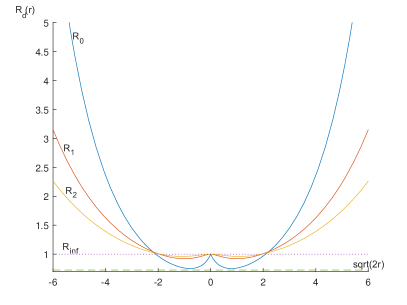
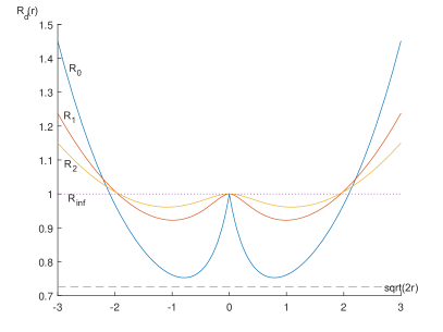
Figure 4: Example of ratio functions $R_{d}(r)={|\kappa_{(d+\frac{1}{2},\rho)}(r)|}/{\kappa_{(d+\frac{3}{2},\rho)}(r)}$ for $d=0,1,2$. Left figure shows wider range, right shows zoom. Note the lower bound (dashed line) $R=0.7529$, local maxima at $r=0$, dual minima at $r=\pm\tilde{r}_{d}$, and divergence as $|r|\to\infty$ for each curve.

We have not been able to prove this postulate. Figure 4 shows $R_{d}(r)$ for $d=0,1,2$, which conforms to the postulate, and we have simulated (and confirmed) the postulate up to $d=83$ (at which point we ran into floating point problems due to the large factorials involved). We note that this far exceeds practical requirements - most practitioners consider only $\nu\in\{\frac{1}{2},\frac{3}{2},\frac{5}{2}\}$ (i.e. $d\in\{0,1,2\}$). $\square$

$d$	$\beta_{d}$	$d$	$\beta_{d}$	$d$	$\beta_{d}$
0	0.752871	22	0.999107	44	0.99976
1	0.92244	23	0.999178	45	0.99977
2	0.96113	24	0.999241	46	0.99978
3	0.976487	25	0.999297	47	0.999789
4	0.984203	26	0.999347	48	0.999797
5	0.988643	27	0.999391	49	0.999805
6	0.991437	28	0.999432	50	0.999813
7	0.993311	29	0.999468	51	0.99982
8	0.99463	30	0.999501	52	0.999826
9	0.995593	31	0.999531	53	0.999833
10	0.996318	32	0.999559	54	0.999839
11	0.996878	33	0.999584	55	0.999844
12	0.997319	34	0.999607	56	0.99985
13	0.997673	35	0.999628	57	0.999855
14	0.997961	36	0.999648	58	0.99986
15	0.998198	37	0.999666	59	0.999864
16	0.998397	38	0.999682	60	0.999869
17	0.998564	39	0.999698	61	0.999873
18	0.998706	40	0.999712	62	0.999877
19	0.998829	41	0.999725	63	0.99988
20	0.998934	42	0.999738	64	0.999884
21	0.999026	43	0.999749	65	0.999887

Table 2: Lower bounds $\beta_{d}$ on Matérn kernel ratios $R_{d}(r)=\frac{\kappa_{(d+\frac{1}{2},\rho)}(r)}{\kappa_{(d+\frac{3}{2},\rho)}(r)}$.

Assuming the postulate is correct we have the following result:

Theorem V

For all $d\in{\mathbb{Z}}_{\infty}\backslash\{0\}$, $q\in{\mathbb{Z}}_{d}+1$, $0\leq r\leq\frac{1}{2}M^{2}$:

$$\begin{array}[]{l}L_{(d+\frac{1}{2},\rho)}^{\downarrow q}{\kappa_{(d+\frac{1}{2},\rho)}\left(r\right)}\leq\left|\kappa_{(d+\frac{1}{2},\rho)}^{(q)}\left(r\right)\right|\leq L_{(d+\frac{1}{2},\rho)}^{\uparrow q}{\kappa_{(d+\frac{1}{2},\rho)}\left(r\right)}\end{array}$$

where:

$$\begin{array}[]{rl}L_{(d+\frac{1}{2},\rho)}^{\downarrow}&\!\!\!=\frac{\sqrt{d+\frac{1}{2}}}{2\rho}0.7528\frac{\sqrt{\pi}}{2\Gamma\left(d+\frac{1}{2}\right)}\\ L_{(d+\frac{1}{2},\rho)}^{\uparrow}&\!\!\!=\frac{\sqrt{d+\frac{1}{2}}}{2\rho}\mathop{\max}\limits_{c\in{\mathbb{Z}}_{d}+1}\left\{1,\frac{\kappa_{d+\frac{1}{2}-c,\rho}\left(\frac{1}{2}M^{2}\right)}{\kappa_{d+\frac{1}{2},\rho}\left(\frac{1}{2}M^{2}\right)}\right\}\end{array}$$

Proof:

Start with (17):

$$\begin{array}[]{rl}\left|\kappa_{(d+\frac{1}{2},\rho)}^{(q)}\left(r\right)\right|&\!\!\!=\left(\left(\frac{\sqrt{d+\frac{1}{2}}}{2\rho}\right)^{q}\frac{\Gamma\left(d+\frac{1}{2}-q\right)}{\Gamma\left(d+\frac{1}{2}\right)}\right)\kappa_{(d+\frac{1}{2}-q,\rho)}\left(r\right)\\ \end{array}$$

and hence:

$$\begin{array}[]{l}\frac{\left|\kappa_{(d+\frac{1}{2},\rho)}^{(q)}\left(r\right)\right|}{\kappa_{(d+\frac{1}{2},\rho)}\left(r\right)}=\left(\frac{\sqrt{d+\frac{1}{2}}}{2\rho}\right)^{q}\frac{\Gamma\left(d+\frac{1}{2}-q\right)}{\Gamma\left(d+\frac{1}{2}\right)}\frac{\kappa_{(d-\frac{1}{2}-q,\rho)}\left(r\right)}{\kappa_{(d+\frac{1}{2},\rho)}\left(r\right)}\end{array}$$

so by postulate IV it follows that, as $0\leq r\leq\frac{1}{2}M^{2}$:

$$\begin{array}[]{rl}\frac{\left|\kappa_{(d+\frac{1}{2},\rho)}^{(q)}\left(r\right)\right|}{\kappa_{(d+\frac{1}{2},\rho)}\left(r\right)}&\!\!\!\leq\left(\frac{\sqrt{d+\frac{1}{2}}}{2\rho}\right)^{q}\frac{\Gamma\left(d+\frac{1}{2}-q\right)}{\Gamma\left(d+\frac{1}{2}\right)}\max\left\{1,\frac{\kappa_{(d+\frac{1}{2}-q,\rho)}\left(\frac{1}{2}M^{2}\right)}{\kappa_{(d+\frac{1}{2},\rho)}\left(\frac{1}{2}M^{2}\right)}\right\}\\ &\!\!\!\leq\left(\frac{\sqrt{d+\frac{1}{2}}}{2\rho}\left(\mathop{\max}\limits_{c\in{\mathbb{Z}}_{d}+1}\left\{1,\frac{\kappa_{(d+\frac{1}{2}-c,\rho)}\left(\frac{1}{2}M^{2}\right)}{\kappa_{(d+\frac{1}{2},\rho)}\left(\frac{1}{2}M^{2}\right)}\right\}\right)^{\frac{1}{q}}\right)^{q}\\ \end{array}$$

and, using postulate IV and recalling that $\Gamma(d+\frac{1}{2})\geq\Gamma(\frac{3}{2})=\frac{1}{2}\sqrt{\pi}$ $\forall d\in{\mathbb{Z}}_{\infty}\backslash\{0\}$, $q\in{\mathbb{Z}}_{d}+1$:

$$\begin{array}[]{rl}\frac{\left|\kappa_{(d+\frac{1}{2},\rho)}^{(q)}\left(r\right)\right|}{\kappa_{(d+\frac{1}{2},\rho)}\left(r\right)}&\!\!\!\geq\frac{\Gamma\left(\frac{3}{2}\right)}{\Gamma\left(d+\frac{1}{2}\right)}\left(\frac{\sqrt{d+\frac{1}{2}}}{2\rho}\right)^{q}\mathop{\prod}\limits_{c\in{\mathbb{Z}}_{q}}\frac{\kappa_{(d-\frac{1}{2}-c,\rho)}\left(r\right)}{\kappa_{(d+\frac{1}{2}-c,\rho)}\left(r\right)}\\ &\!\!\!\geq\left(\left(\frac{\sqrt{\pi}}{2\Gamma\left(d+\frac{1}{2}\right)}\right)^{\frac{1}{q}}\frac{\sqrt{d+\frac{1}{2}}}{2\rho}\right)^{q}\left(\mathop{\min}\limits_{\tilde{r}\geq 0,c\in{\mathbb{Z}}_{q}}\frac{\kappa_{(d-\frac{1}{2}-c,\rho)}\left(\tilde{r}\right)}{\kappa_{(d+\frac{1}{2}-c,\rho)}\left(\tilde{r}\right)}\right)^{q}\\ &\!\!\!\geq\left(\frac{\sqrt{d+\frac{1}{2}}}{2\rho}0.7528\left(\frac{\sqrt{\pi}}{2\Gamma\left(d+\frac{1}{2}\right)}\right)^{\frac{1}{q}}\right)^{q}\\ \end{array}$$

and so:

$$\begin{array}[]{l}L_{(q);(d+\frac{1}{2},\rho)}^{\downarrow q}{\kappa_{(d+\frac{1}{2},\rho)}\left(r\right)}\leq\left|\kappa_{(d+\frac{1}{2},\rho)}^{(q)}\left(r\right)\right|\leq L_{(q);(d+\frac{1}{2},\rho)}^{\uparrow q}{\kappa_{(d+\frac{1}{2},\rho)}\left(r\right)}\end{array}$$

where:

$$\begin{array}[]{rl}L_{(q);(d+\frac{1}{2},\rho)}^{\downarrow}&\!\!\!=\frac{\sqrt{d+\frac{1}{2}}}{2\rho}0.7528\left(\frac{\sqrt{\pi}}{2\Gamma\left(d+\frac{1}{2}\right)}\right)^{\frac{1}{q}}\\ L_{(q);(d+\frac{1}{2},\rho)}^{\uparrow}&\!\!\!=\frac{\sqrt{d+\frac{1}{2}}}{2\rho}\left(\mathop{\max}\limits_{c\in{\mathbb{Z}}_{d}+1}\left\{1,\frac{\kappa_{(d+\frac{1}{2}-c,\rho)}\left(\frac{1}{2}M^{2}\right)}{\kappa_{(d+\frac{1}{2},\rho)}\left(\frac{1}{2}M^{2}\right)}\right\}\right)^{\frac{1}{q}}\end{array}$$

As $\Gamma(d+\frac{1}{2})\geq\Gamma(\frac{3}{2})=\frac{1}{2}\sqrt{\pi}$ $\forall d\in{\mathbb{Z}}_{\infty}\backslash\{0\}$ for $q\in{\mathbb{Z}}_{d}+1$ we have:

$$\begin{array}[]{rl}L_{(q);(d+\frac{1}{2},\rho)}^{\downarrow}&\!\!\!=\frac{\sqrt{d+\frac{1}{2}}}{2\rho}0.7528\left(\frac{\sqrt{\pi}}{2\Gamma\left(d+\frac{1}{2}\right)}\right)^{\frac{1}{q}}\geq L_{(d+\frac{1}{2},\rho)}^{\downarrow}\\ L_{(q);(d+\frac{1}{2},\rho)}^{\uparrow}&\!\!\!=\frac{\sqrt{d+\frac{1}{2}}}{2\rho}\left(\mathop{\max}\limits_{c\in{\mathbb{Z}}_{d}+1}\left\{1,\frac{\kappa_{(d+\frac{1}{2}-c,\rho)}\left(\frac{1}{2}M^{2}\right)}{\kappa_{(d+\frac{1}{2},\rho)}\left(\frac{1}{2}M^{2}\right)}\right\}\right)^{\frac{1}{q}}\leq L_{(d+\frac{1}{2},\rho)}^{\uparrow}\\ \end{array}$$

and the result follows. $\square$

Finally we note that the remainders of the Taylor expansion of the Matérn kernels do not converge as the derivatives exist only to finite order (excepting the case $\nu\to\infty$, which corresponds to the RBF kernel). The remainders $\Delta_{(d+\frac{1}{2},\rho)r}(\delta r)$ and $\Delta_{(d+\frac{1}{2},\rho)}(\delta r)$ appear non-trivial to calculate, and we have been unable to find a closed-form bound. Section D discusses how these may be approximated.

C.3 A Counter-Example: the Rational Quadratic Kernel

The rational quadric kernel is defined by [5]:

$$\begin{array}[]{l}K\left({\bf x},{\bf x}^{\prime}\right)=\kappa_{(\theta)}\left(\frac{1}{2}\left\|{\bf x}-{\bf x}^{\prime}\right\|_{2}^{2}\right)\end{array}$$

where $\theta\in{\mathbb{R}}_{+}$ and:

$$\begin{array}[]{l}\kappa_{(\theta)}\left(r\right)=\frac{\theta}{2r+\theta}\end{array}$$

We see immediately that $K\in{\mathbb{C}}_{\infty}$, and $\forall q\in{\mathbb{Z}}_{\infty}$:

$$\begin{array}[]{rl}\kappa_{(\theta)}^{(q)}\left(r\right)&\!\!\!=\frac{\partial^{q}}{\partial r^{q}}\kappa_{(\theta)}\left(r\right)=\left(-2\right)^{q}q!\frac{\theta}{\left(2r+\theta\right)^{q+1}}\end{array}$$

However when we attempt to find $L_{(\theta)}^{\uparrow}$, $L_{(\theta)}^{\downarrow}$ to satisfy assumption 4 - that is, $L_{(\theta)}^{\uparrow}$, $L_{(\theta)}^{\downarrow}$ satisfying:

$$\begin{array}[]{l}L_{(\theta)}^{\downarrow}\leq\left(\frac{\left|\kappa_{(\theta)}^{(q)}\left(r\right)\right|}{\kappa_{(\theta)}\left(r\right)}\right)^{\frac{1}{q}}=\left(q!\right)^{\frac{1}{q}}\frac{2}{2r+\theta}\leq L_{(\theta)}^{\uparrow}\end{array}$$

we immediately see that no such can exist, as the central term grows factorially with $q$, so $L_{(\theta)}^{\uparrow},L_{(\theta)}^{\downarrow}\to\infty$; and while we may artificially bound the differentiability to $s<\infty$, the resulting bound on the remainders of the Taylor expansion of $f$ (see theorem 3) will grow exponentially with $s$ as:

$$\begin{array}[]{l}\left|R_{q:{\bf x}}\left(\delta{\bf x}\right)\right|\leq U_{p}\left(B\right)\propto D^{\uparrow}\propto e^{\frac{1}{2}L_{(\theta)}^{\uparrow}}\propto e^{\frac{1}{2}\left(s!\right)^{\frac{1}{s}}}\end{array}$$

rendering the bound useless in this particular case and making the rational quadratic kernel unsuitable for our purposes here.

Appendix D A Note on the Estimation of the Intrinsic Remainders $\Delta_{r}\left(\delta r\right)$ and $\Delta\left(r\right)$ for Non-Convergent Kernels

In the previous section the Matérn kernels discussed have non-convergent Taylor expansions and hence non-zero intrinsic remainders $\Delta_{r}(\delta r)$ and $\Delta(\delta r)$ (that is, one cannot obtain an arbitrarily accurate approximation of $\kappa(r+\delta r)$ by simply extending the Taylor series about $r$ to arbitrary order). We also noted that these remainders may be difficult to bound (tightly) in closed-form. In this section we discuss how they may be approximated using a simple Monte-Carlo approach [4].

We proceed as follows. Let $K({\bf x},{\bf x}^{\prime})=\kappa(\frac{1}{2}\|{\bf x}-{\bf x}^{\prime}\|_{2}^{2})$ be an $s$-times differentiable isotropic kernel, where $s$ is finite. Define:

$$\begin{array}[]{l}E_{r}\left(\delta r\right)=\left|\kappa\left(r+\delta r\right)-\mathop{\sum}\limits_{q\in{\mathbb{Z}}_{d+1}}\frac{1}{q!}\delta r^{q}\kappa^{(q)}\left(r\right)\right|\\ \end{array}$$

to be the actual (tight) remainder bound on the Taylor expansion of $\kappa$ about $r$ to maximal order $s$ (for example if we are using a Matérn kernel of order $\frac{5}{2}$ then $s=2$, so this is easily calculated).

The intrinsic remainder bound $\Delta_{r}(\delta r)$ must satisfy:

1. Remainder bound: $\Delta_{r}(\delta r)\geq E_{r}(\delta r)$ $\forall\delta r\geq 0$.

2. Non-decreasing: $\Delta_{r}(\delta r)\geq\Delta_{r}(\delta s)$ $\forall\delta s\in[0,\delta r]$.

It follows that we may estimate a lower bound on $\Delta_{r}(\delta r)$ by sampling:

$$\begin{array}[]{l}\Delta_{r}\left(\delta r\right)\approx\max\left\{\left.E_{r}\left(\delta r\right),E_{r}\left(s_{i}\right)\right|s_{0},s_{1},\ldots,s_{R_{A}}\sim{\mathcal{U}}\left(0,\delta r\right)\right\}\end{array}$$

where the number of samples $R_{A}$ controls the accuracy of this estimate. Moreover we can use the same approach to approximate $\Delta(\delta r)$:

$$\begin{array}[]{rl}\Delta\left(\delta r\right)&\!\!\!=\mathop{\max}\limits_{r\in\left[0,\frac{1}{2}M^{2}\right]}\frac{\Delta_{r}\left(\delta r\right)}{\kappa\left(r\right)}\\ &\!\!\!\approx\max\left\{\left.\frac{\Delta_{r_{i}}\left(\delta r\right)}{\kappa\left(r\right)}\right|r_{0},r_{1},\ldots,r_{R_{B}}\sim{\mathcal{U}}\left(0,\frac{1}{2}M^{2}\right)\right\}\\ \end{array}$$

where the number of meta-samples $R_{B}$ controls the accuracy of this estimate along with $R_{A}$.

The total number of samples required to approximate $\Delta(\delta r)$ in this scheme is $R_{A}R_{B}$. This may seem large if good accuracy is desired, but it is only required twice in the Bayesian optimisation algorithm - once to calculate $p_{\rm min}$, once to calculate $U_{p}(B)$ - so in practice this presents no real difficulty.

Appendix E Proof of Theorem 5

Before proceding with the proof of theorem 5 we first prove the Theorem:

Theorem VI (Expected Stable Gain)

Let ${\mathbb{D}}=\{({\bf x}_{i},{y}_{i})|{y}_{i}=f({\bf x}_{i})+\epsilon_{i}\}$, and ${\mathbb{F}}=\{(\tilde{\bf x}_{i},\tilde{y}_{i})|\tilde{y}_{i}=f(\tilde{\bf x}_{i})+\tilde{\epsilon}_{i}\}$. Assume without loss of generality that $\tilde{y}_{0}\leq\tilde{y}_{1}\leq\ldots$ and define $\tilde{y}_{-1}=\chi$. Given:

$$\begin{array}[]{l}\nabla_{\bf x}^{(q)}f\left({\bf x}\right)\sim{\mathcal{N}}\left({\bf m}_{\mathbb{D}}^{(q)}\left({\bf x}\right),{\mbox{\boldmath$\Lambda$}}^{(q)}\left({\bf x},{\bf x}\right)\right)\end{array}$$

the expected stable gain of ${\mathbb{F}}$ given ${\mathbb{D}}$ is:

$$\begin{array}[]{rl}\mathrm{E}\left(\left.g_{{\mu}}\left({\mathbb{F}}\right)\right|{\mathbb{D}}\right)&\!\!\!=\mathop{\sum}\limits_{i\in{\mathbb{Z}}_{|{\mathbb{F}}|}}\left(\tilde{y}_{i}-\tilde{y}_{i-1}\right)\left(1-\mathop{\prod}\limits_{j\in{\mathbb{Z}}_{|{\mathbb{F}}|}\backslash{\mathbb{Z}}_{i}}\left(1-s_{{{\mu}_{1:p}}}\left(\left.\tilde{\bf x}_{j}\right|{\mathbb{D}}\right)\right)\right)\\ \end{array}$$

Proof:

Using the fact that $f$ is a draw from a Gaussian Process, defining ${\bf v}_{j}^{(q)}\sim{\mathcal{N}}(\frac{B^{q}}{q!}{\bf m}_{\mathbb{D}}^{(q)}(\tilde{\bf x}_{j}),(\frac{B^{q}}{q!})^{2}{\mbox{\boldmath$\Lambda$}}_{\mathbb{D}}^{(q)}(\tilde{\bf x}_{j},\tilde{\bf x}_{j}))$ $\forall j$ and applying Theorem 2:

$$\begin{array}[]{rl}\mathrm{E}\left(\left.g_{{\mu}}\left({\mathbb{F}}\right)\right|{\mathbb{D}}\right)&\!\!\!=\mathrm{E}\left(\int_{\chi}^{\infty}\mathbbold{1}\left({\exists\left(\tilde{\bf x}_{j},\tilde{y}_{j}\right)\in{\mathbb{F}}\left|\tilde{y}_{j}\geq y\wedge\tilde{\bf x}_{i}\in{\mathbb{S}}_{{{\mu}_{1:p}}}\right.}\right)dy\right)\\ &\!\!\!=\mathop{\sum}\limits_{i\in{\mathbb{Z}}_{|{\mathbb{F}}|}}\int_{y_{i-1}}^{y_{i}}\Pr\left(\mathop{\bigvee}\limits_{j\in{\mathbb{Z}}_{|{\mathbb{F}}|}\backslash{\mathbb{Z}}_{i}}\left(\mathop{\bigwedge}\limits_{q\in{\mathbb{Z}}_{p}+1}\left\|{\bf v}_{j}^{(q)}\right\|_{\bullet}\leq{\mu}\right)\right)dy\\ &\!\!\!=\mathop{\sum}\limits_{i\in{\mathbb{Z}}_{|{\mathbb{F}}|}}\left(\tilde{y}_{i}-\tilde{y}_{i-1}\right)\left(1-\mathop{\prod}\limits_{j\in{\mathbb{Z}}_{|{\mathbb{F}}|}\backslash{\mathbb{Z}}_{i}}\left(1-s_{{{\mu}_{1:p}}}\left(\left.\tilde{\bf x}_{j}\right|{\mathbb{D}}\right)\right)\right)\\ \end{array}$$

where the range of the product arises from the assumed ordering on $\tilde{y}_{i}$. $\square$

Having established the preliminary we now prove the theorem:

Theorem 5

Let ${\mathbb{D}}=\{({\bf x}_{i},{y}_{i})|{y}_{i}=f({\bf x}_{i})+\epsilon_{i}\}$. Assume without loss of generality that ${y}_{0}\leq{y}_{1}\leq\ldots$ and define $y_{-1}=\chi$, $y_{|{\mathbb{D}}|}=\infty$. Given:

$$\begin{array}[]{l}f\left({\bf x}\right)\sim{\mathcal{N}}\left(m_{\mathbb{D}}\left({\bf x}\right),\lambda_{\mathbb{D}}\left({\bf x},{\bf x}\right)\right)\\ \nabla_{\bf x}^{(q)}f\left({\bf x}\right)\sim{\mathcal{N}}\left({\bf m}_{\mathbb{D}}^{(q)}\left({\bf x}\right),{\mbox{\boldmath$\Lambda$}}^{(q)}\left({\bf x},{\bf x}\right)\right)\end{array}$$

the EISG acquisition function reduces to:

$$\begin{array}[]{l}a^{{\rm EISG}}\left({\bf x}|{\mathbb{D}}\right)=\lambda^{1/2}_{\mathbb{D}}\left({\bf x},{\bf x}\right)s_{{{\mu}_{1:p}}}\left(\left.{\bf x}\right|{\mathbb{D}}\right)\ldots\\ \ldots\mathop{\sum}\limits_{k\in{\mathbb{Z}}_{|{\mathbb{D}}|+1}}\Big{(}\Delta\Phi_{k}\left({\bf x}\right)\mathop{\sum}\limits_{i\in{\mathbb{Z}}_{{k}}}\omega_{i}\Delta\hat{y}_{i}\left({\bf x}\right)+\ldots\\ \;\;\;\;\;\;\;\;\ldots+\omega_{k}\left(z_{k-1}\left({\bf x}\right)\Delta\Phi_{k}\left({\bf x}\right)+\Delta\phi_{k}\left({\bf x}\right)\right)\Big{)}\end{array}$$

where $z_{i}({\bf x})=\frac{m_{\mathbb{D}}({\bf x})-y_{i}}{\lambda^{1/2}_{\mathbb{D}}({\bf x},{\bf x})}$, $\Delta\hat{y}_{i}({\bf x})=\frac{{y}_{i}-{y}_{i-1}}{\lambda^{1/2}_{{\mathbb{D}}}({\bf x},{\bf x})}$ and:

$$\begin{array}[]{l}\Delta\phi_{k}\left({\bf x}\right)=\phi\left(z_{k-1}\left({\bf x}\right)\right)-\phi\left(z_{k}\left({\bf x}\right)\right)\\ \Delta\Phi_{k}\left({\bf x}\right)=\Phi\left(z_{k-1}\left({\bf x}\right)\right)-\Phi\left(z_{k}\left({\bf x}\right)\right)\\ \end{array}$$

so $\Delta\Phi_{|{\mathbb{D}}|}({\bf x})=\Phi(z_{|{\mathbb{D}}|-1}({\bf x}))$ and $\Delta\phi_{|{\mathbb{D}}|}({\bf x})=\phi(z_{|{\mathbb{D}}|-1}({\bf x}))$. The weights $\omega_{0}$, $\omega_{1}$, $\ldots$, $\omega_{|{\mathbb{D}}|}$ are given by:

$$\begin{array}[]{l}\omega_{|{\mathbb{D}}|}=1\\ \omega_{i}=\omega_{i+1}\left(1-s_{{{\mu}_{1:p}}}\left(\left.{\bf x}_{i+1}\right|{\mathbb{D}}\right)\right)\;\forall i\in{\mathbb{Z}}_{|{\mathbb{D}}|}\\ \end{array}$$

Proof:

Working from the definition of EISG:

$$\begin{array}[]{l}a^{{\rm EISG}}\left({\bf x}|{\mathbb{D}}\right)\;\;\;=\mathrm{E}\left(g_{{{\mu}_{1:p}}}\left({\mathbb{D}}\cup\left\{\left({\bf x},y\right)\right\}\right)-g_{{{\mu}_{1:p}}}\left({\mathbb{D}}\right)\right)\\ \;\;\;=\mathrm{E}_{f}\left(\mathrm{E}_{\nabla_{\bf x}^{\otimes q}}\left(g_{{{\mu}_{1:p}}}\left({\mathbb{D}}\cup\left\{\left({\bf x},y\right)\right\}\right)\right)-\mathrm{E}_{\nabla_{\bf x}^{\otimes q}}\left(g_{{{\mu}_{1:p}}}\left({\mathbb{D}}\right)\right)\right)\\ \;\;\;=\int_{\chi}^{\infty}\left(\mathrm{E}_{\nabla_{\bf x}^{\otimes q}}\left(\left.g_{{{\mu}_{1:p}}}\left({\mathbb{D}}\cup\left\{\left({\bf x},y\right)\right\}\right)\right|{\mathbb{D}}\right)-\mathrm{E}_{\nabla_{\bf x}^{\otimes q}}\left(\left.g_{{{\mu}_{1:p}}}\left({\mathbb{D}}\right)\right|{\mathbb{D}}\right)\right)\phi\left(\frac{y-m_{\mathbb{D}}\left({\bf x}\right)}{\kappa_{\mathbb{D}}^{1/2}\left({\bf x},{\bf x}\right)}\right)dy\\ \;\;\;=\mathop{\sum}\limits_{k\in{\mathbb{Z}}_{|{\mathbb{D}}|+1}}a^{{\rm EISG}}_{k}\left({\bf x}|{\mathbb{D}}\right)\end{array}$$

where the outer expectation is with regard to $f({\bf x})\sim{\mathcal{N}}(m_{\mathbb{D}}({\bf x}),\lambda_{\mathbb{D}}({\bf x},{\bf x}))$ and the inner expectation with regard to $\nabla_{\bf x}^{(q)}f({\bf x})\sim{\mathcal{N}}({\bf m}_{\mathbb{D}}^{(q)}({\bf x}),{\mbox{\boldmath$\Lambda$}}^{(q)}({\bf x},{\bf x}))$, and we have defined:

$$\begin{array}[]{l}a^{{\rm EISG}}_{k}\left({\bf x}|{\mathbb{D}}\right)=\int_{y_{k-1}}^{y_{k}}\left(\mathrm{E}_{\nabla_{\bf x}^{\otimes q}}\left(\left.g_{{{\mu}_{1:p}}}\left({\mathbb{D}}\cup\left\{\left({\bf x},y\right)\right\}\right)\right|{\mathbb{D}}\right)-\mathrm{E}_{\nabla_{\bf x}^{\otimes q}}\left(\left.g_{{{\mu}_{1:p}}}\left({\mathbb{D}}\right)\right|{\mathbb{D}}\right)\right)\phi\left(\frac{y-m_{\mathbb{D}}\left({\bf x}\right)}{\kappa_{\mathbb{D}}^{1/2}\left({\bf x},{\bf x}\right)}\right)dy\\ \end{array}$$

Using Lemma VI:

$$\begin{array}[]{l}\mathrm{E}\left(\left.g_{{{\mu}_{1:p}}}\left({\mathbb{D}}\right)\right|{\mathbb{D}}\right)=\mathop{\sum}\limits_{i\in{\mathbb{Z}}_{{|{\mathbb{D}}|}}}\left({y}_{i}-{y}_{i-1}\right)\left(1-\mathop{\prod}\limits_{j\in{\mathbb{Z}}_{{|{\mathbb{D}}|}}\backslash{\mathbb{Z}}_{i}}\left(1-s_{{{\mu}_{1:p}}}\left(\left.{\bf x}_{j}\right|{\mathbb{D}}\right)\right)\right)\\ \end{array}$$

and hence $\forall k\in{\mathbb{Z}}_{|{\mathbb{D}}|+1}$:

$$\begin{array}[]{l}\int_{y_{k-1}}^{y_{k}}\mathrm{E}\left(\left.g_{{{\mu}_{1:p}}}\left({\mathbb{D}}\right)\right|{\mathbb{D}}\right)\phi\left(\frac{y-m_{\mathbb{D}}\left({\bf x}\right)}{\kappa^{1/2}_{\mathbb{D}}\left({\bf x},{\bf x}\right)}\right)dy=\Delta\Phi_{k}\left({\bf x}\right)\mathop{\sum}\limits_{i\in{\mathbb{Z}}_{{|{\mathbb{D}}|}}}\left({y}_{i}-{y}_{i-1}\right)\left(1-\omega_{i}\right)\\ \end{array}$$

and:

$$\begin{array}[]{l}\int_{y_{k-1}}^{y_{k}}\mathrm{E}\left(\left.g_{{{\mu}_{1:p}}}\left({\mathbb{D}}\cup\left\{\left({\bf x},y\right)\right\}\right)\right|{\mathbb{D}}\right)\phi\left(\frac{y-m_{\mathbb{D}}\left({\bf x}\right)}{\kappa^{1/2}_{\mathbb{D}}\left({\bf x},{\bf x}\right)}\right)dy\\ =\Delta\Phi_{k}\left({\bf x}\right)\mathop{\sum}\limits_{i\in{\mathbb{Z}}_{k}}\left({y}_{i}-{y}_{i-1}\right)\left(1-\left(1-s_{{{\mu}_{1:p}}}\left(\left.{\bf x}\right|{\mathbb{D}}\right)\right)\mathop{\prod}\limits_{j\in{\mathbb{Z}}_{{|{\mathbb{D}}|}}\backslash{\mathbb{Z}}_{i}}\left(1-s_{{{\mu}_{1:p}}}\left(\left.{\bf x}_{j}\right|{\mathbb{D}}\right)\right)\right)+\ldots\\ \;\;\;+\;\left(\int_{y_{k-1}}^{y_{k}}\left(y-y_{k-1}\right)\phi\left(\frac{y-m_{\mathbb{D}}\left({\bf x}\right)}{\kappa^{1/2}_{\mathbb{D}}\left({\bf x},{\bf x}\right)}\right)dy\right)\left(1-\left(1-s_{{{\mu}_{1:p}}}\left({\bf x}\right)\right)\mathop{\prod}\limits_{j\in{\mathbb{Z}}_{{|{\mathbb{D}}|}}\backslash{\mathbb{Z}}_{k}}\left(1-s_{{{\mu}_{1:p}}}\left(\left.{\bf x}_{j}\right|{\mathbb{D}}\right)\right)\right)+\ldots\\ \;\;\;+\;\left(\int_{y_{k-1}}^{y_{k}}\left(y_{k}-y\right)\phi\left(\frac{y-m_{\mathbb{D}}\left({\bf x}\right)}{\kappa^{1/2}_{\mathbb{D}}\left({\bf x},{\bf x}\right)}\right)dy\right)\mathop{\sum}\left(1-\mathop{\prod}\limits_{j\in{\mathbb{Z}}_{{|{\mathbb{D}}|}}\backslash{\mathbb{Z}}_{k}}\left(1-s_{{{\mu}_{1:p}}}\left(\left.{\bf x}_{j}\right|{\mathbb{D}}\right)\right)\right)+\ldots\\ \;\;\;+\;\Delta\Phi_{k}\left({\bf x}\right)\mathop{\sum}\limits_{i\in{\mathbb{Z}}_{{|{\mathbb{D}}|}}\backslash{\mathbb{Z}}_{k}}\left({y}_{i}-{y}_{i-1}\right)\left(1-\mathop{\prod}\limits_{j\in{\mathbb{Z}}_{{|{\mathbb{D}}|}}\backslash{\mathbb{Z}}_{i}}\left(1-s_{{{\mu}_{1:p}}}\left(\left.{\bf x}_{j}\right|{\mathbb{D}}\right)\right)\right)\\ =\Delta\Phi_{k}\left({\bf x}\right)\mathop{\sum}\limits_{i\in{\mathbb{Z}}_{k}}\left({y}_{i}-{y}_{i-1}\right)\left(1-\left(1-s_{{{\mu}_{1:p}}}\left(\left.{\bf x}\right|{\mathbb{D}}\right)\right)\omega_{i}\right)+\ldots\\ \;\;\;+\;\kappa^{1/2}_{\mathbb{D}}\left({\bf x},{\bf x}\right)\Delta\phi_{k}\left({\bf x}\right)+z_{k-1}\left({\bf x}\right)\Delta\Phi_{k}\left({\bf x}\right)\left(1-\left(1-s_{{{\mu}_{1:p}}}\left(\left.{\bf x}\right|{\mathbb{D}}\right)\right)\omega_{k}\right)+\ldots\\ \;\;\;-\;\kappa^{1/2}_{\mathbb{D}}\left({\bf x},{\bf x}\right)\Delta\phi_{k}\left({\bf x}\right)+z_{k}\left({\bf x}\right)\Delta\Phi_{k}\left({\bf x}\right)\left(1-\omega_{k}\right)+\ldots\\ \;\;\;+\;\Delta\Phi\left({\bf x}\right)\mathop{\sum}\limits_{i\in{\mathbb{Z}}_{{|{\mathbb{D}}|}}\backslash{\mathbb{Z}}_{k}}\left({y}_{i}-{y}_{i-1}\right)\left(1-\omega_{i}\right)\\ =\kappa^{1/2}_{\mathbb{D}}\left({\bf x},{\bf x}\right)s_{{{\mu}_{1:p}}}\left(\left.{\bf x}\right|{\mathbb{D}}\right)\Delta\Phi_{k}\left({\bf x}\right)\mathop{\sum}\limits_{i\in{\mathbb{Z}}_{k}}\omega_{i}\Delta\hat{y}_{i}\left({\bf x}\right)+\ldots\\ \;\;\;+\;\Delta\Phi_{k}\left({\bf x}\right)\mathop{\sum}\limits_{i\in{\mathbb{Z}}_{k}}\left({y}_{i}-{y}_{i-1}\right)\left(1-\omega_{i}\right)+\ldots\\ \;\;\;+\;\kappa^{1/2}_{\mathbb{D}}\left({\bf x},{\bf x}\right)s_{{{\mu}_{1:p}}}\left(\left.{\bf x}\right|{\mathbb{D}}\right)\left(\Delta\phi_{k}\left({\bf x}\right)+z_{k-1}\left({\bf x}\right)\Delta\Phi_{k}\left({\bf x}\right)\right)\omega_{k}+\ldots\\ \;\;\;+\;\kappa^{1/2}_{\mathbb{D}}\left({\bf x},{\bf x}\right)\left(\Delta\phi_{k}\left({\bf x}\right)+z_{k-1}\left({\bf x}\right)\Delta\Phi_{k}\left({\bf x}\right)\right)\left(1-\omega_{k}\right)+\ldots\\ \;\;\;-\;\kappa^{1/2}_{\mathbb{D}}\left({\bf x},{\bf x}\right)\left(\Delta\phi_{k}\left({\bf x}\right)+z_{k}\left({\bf x}\right)\Delta\Phi_{k}\left({\bf x}\right)\right)\left(1-\omega_{k}\right)+\ldots\\ \;\;\;+\;\Delta\Phi_{k}\left({\bf x}\right)\mathop{\sum}\limits_{i\in{\mathbb{Z}}_{{|{\mathbb{D}}|}}\backslash{\mathbb{Z}}_{k}}\left({y}_{i}-{y}_{i-1}\right)\left(1-\omega_{i}\right)\\ =\Delta\Phi_{k}\left({\bf x}\right)\mathop{\sum}\limits_{i\in{\mathbb{Z}}_{k}}\left({y}_{i}-{y}_{i-1}\right)\left(1-\omega_{i}\right)+\Delta\Phi_{k}\left({\bf x}\right)\left(y_{k}-y_{k-1}\right)\left(1-\omega_{k}\right)+\ldots\\ \;\;\;+\;\Delta\Phi_{k}\left({\bf x}\right)\mathop{\sum}\limits_{i\in{\mathbb{Z}}_{{|{\mathbb{D}}|}}\backslash{\mathbb{Z}}_{k}}\left({y}_{i}-{y}_{i-1}\right)\left(1-\omega_{i}\right)+\ldots\\ \;\;\;+\;\kappa^{1/2}_{\mathbb{D}}\left({\bf x},{\bf x}\right)s_{{{\mu}_{1:p}}}\left(\left.{\bf x}\right|{\mathbb{D}}\right)\Delta\Phi_{k}\left({\bf x}\right)\mathop{\sum}\limits_{i\in{\mathbb{Z}}_{k}}\omega_{i}\Delta\hat{y}_{i}\left({\bf x}\right)+\ldots\\ \;\;\;+\;\kappa^{1/2}_{\mathbb{D}}\left({\bf x},{\bf x}\right)s_{{{\mu}_{1:p}}}\left(\left.{\bf x}\right|{\mathbb{D}}\right)\left(\Delta\phi_{k}\left({\bf x}\right)+z_{k-1}\left({\bf x}\right)\Delta\Phi_{k}\left({\bf x}\right)\right)\omega_{k}\\ =\int_{y_{k-1}}^{y_{k}}\mathrm{E}\left(\left.g_{{{\mu}_{1:p}}}\left({\mathbb{D}}\right)\right|{\mathbb{D}}\right)\phi\left(\frac{y-m_{\mathbb{D}}\left({\bf x}\right)}{\kappa^{1/2}_{\mathbb{D}}\left({\bf x},{\bf x}\right)}\right)dy+\ldots\\ \;\;\;+\;\kappa^{1/2}_{\mathbb{D}}\left({\bf x},{\bf x}\right)s_{{{\mu}_{1:p}}}\left(\left.{\bf x}\right|{\mathbb{D}}\right)\Bigg{(}\Delta\Phi_{k}\left({\bf x}\right)\mathop{\sum}\limits_{i\in{\mathbb{Z}}_{k}}\omega_{i}\Delta\hat{y}_{i}\left({\bf x}\right)+\omega_{k}\left(z_{k-1}\left({\bf x}\right)\Delta\Phi_{k}\left({\bf x}\right)+\Delta\phi_{k}\left({\bf x}\right)\right)\Bigg{)}\\ \end{array}$$

and the first result follows by summing over all $k$.

The recursive form of the weights $\omega_{i}$ may be deduced by inspection, using the convention that the empty product evaluates to $1$. $\square$

References

- [1] Milton Abramowitz, Irene A. Stegun, and Donald A. McQuarrie. Handbook of Mathematical Functions with Formulas, Graphs, and Mathematical Tables. Dover, 1972.
- [2] John P. Boyd. Asymptotic coefficients of hermite function series. Journal of Computational Physics, 54:382–410, 1984.
- [3] Eric Brochu, Vlad M. Cora, and Nando de Freitas. A tutorial on bayesian optimization of expensive cost functions, with applications to active user modeling and heirarchical reinforcement learning. eprint arXiv:1012.2599, arXiv.org, December 2010.
- [4] Pierre Del Moral, Arnaud Doucet, and Ajay Jasra. Sequential monte carlo samplers. Journal of the Royal Statistical Society: Series B (Statistical Methodology), 68(3):411–436, 2006.
- [5] Marc G. Genton. Classes of kernels for machine learning: A statistics perspective. Journal of Machine Learning Research, 2:299–312, 2001.
- [6] José Miguel Hernández-Lobato, Matthew Hoffman, and Zoubin Ghahramani. Predictive entropy search for efficient global optimization of black-box functions. In NIPS, pages 918–926, 2014.
- [7] Donald R. Jones, Matthias Schonlau, and William J. Welch. Efficient global optimization of expensive black-box functions. Journal of Global optimization, 13(4):455–492, 1998.
- [8] David J. C. MacKay. Introduction to gaussian processes. NATO ASI Series F Computer and Systems Sciences, 168, 1998.
- [9] Andrew McHutchon. Differentiating gaussian processes. Cambridge (ed.), 2013.
- [10] Tanh Dai Nguyen, Sunil Gupta, Santu Rana, and Svetha Venkatesh. Stable bayesian optimization. International Journal of Data Science and Analytics, 6(4):327–339, 2018.
- [11] Thanh Dai Nguyen, Sunil Gupta, Santu Rana, and Svetha Venkatesh. Stable bayesian optimization. In PAKDD 2017: Advances in Knowledge Discovery and Data Mining: Proceedings of the 21st Pacific-Asia Conference, pages 578–591. Springer International Publishing, 2017.
- [12] José Nogueira, Ruben Martinez-Cantin, Alexandre Bernardina, and Lorenzo Jamone. Unscented bayesian optimization for safe robot grasping. In Proceedings of the IEEE/RSJ International Conference on Intelligent Robots and Systems IROS, 2016.
- [13] A. O’Hagan. Some bayesian numerical analysis. Bayesian Statistics, 7:345–363, 1992.
- [14] Carl Edward Rasmussen. Gaussian processes to speed up hybrid monte carlo for expensive bayesian integrals. Bayesian statistics, 7:651–659, 2008.
- [15] Carl Edward Rasmussen and Christopher K. I. Williams. Gaussian Processes for Machine Learning. MIT Press, 2006.
- [16] Herbert Robbins. A remark on stirling’s formula. The American Mathematical Monthly, 62(1):26–29, 1955.
- [17] Ercan Solak, Roderick Murray-Smith, William E. Leithead, Douglas J. Leith, and Carl E. Rasmussen. Derivative observations in gaussian process models of dynamic systems. In Advances in neural information processing systems, pages 1057–1064, 2003.
- [18] Niranjan Srinivas, Andreas Krause, Sham M. Kakade, and Matthias W. Seeger. Information-theoretic regret bounds for gaussian process optimization in the bandit setting. IEEE Transactions on Information Theory, 58(5):3250–3265, May 2012.
- [19] Anqi Wu, Mikio C. Aoi, and Jonathan W. Pillow. Exploiting gradients and hessians in bayesian optimization and bayesian quadrature. arXiv preprint arXiv:1704.00060, 2017.