Few-body systems in condensed matter physics.

Abstract

This review focuses on the studies and computations of few-body systems of electrons and holes in condensed matter physics. We analyze and illustrate the application of a variety of methods for description of two- three- and four-body excitonic complexes such as an exciton, trion and biexciton in three-, two- and one-dimensional configuration spaces in various types of materials. We discuss and analyze the contributions made over the years to understanding how the reduction of dimensionality affects the binding energy of excitons, trions and biexcitons in bulk and low-dimensional semiconductors and address the challenges that still remain.

I
Introduction

Over the past 50 years, the physics of few-body systems has received substantial development. Starting from the mid-1950’s, the scientific community has made great progress and success towards the development of methods of theoretical physics for the solution of few-body problems in physics. In 1957,  Skornyakov and Ter-Martirosyan TerMartiros solved the quantum three-body problem and derived equations for the determination of the wave function of a system of three identical particles (fermions) in the limiting case of zero-range forces. The integral equation approach TerMartiros was generalized by Faddeev Faddeev to include finite and long range interactions. It was shown that the eigenfunctions of the Hamiltonian of a three-particle system with pair interaction can be represented in a natural fashion as the sum of three terms, for each of which there exists a coupled set of equations. It should be noted that the natural division of the wave function in the three-particle problem into three terms had also been considered earlier by Eyges Eyges and Gribov Gribov . However, by using this division of the wave function in the three particle problem into three terms Faddeev obtained a set of integral equations with an unambiguous solution. In the limit of zero range, one obtains the well-known Skornyakov-Ter-Martirosyan equations TerMartiros . The introduction of separable potentials allowed us to turn the problem of finding the amplitudes to that of solving a one-dimensional integral equation. The complete mathematical study and investigation of three-body problem in discrete and continuum spectra was done by L. D. Faddeev in Ref. FaddeevTrudi . ”Those days Faddeev was already a prominent figure in quantum physics” Efimov2019 . The studies of three-body physics led to discovery of the Efimov’s effect Efimov1970 ; Efimov1970PL . When Efimov in 1970 discussed this phenomenon with Faddeev, ”Faddeev was very surprised. In a few days he [Faddeev] called me [Efimov] and said he confirmed my results using his own method” Efimov2019 .

As for the four-body system, Faddeev’s idea of an explicit cluster-channel separation was completely elaborated by Yakubovsky in 1967 Yakubovsky . Merkuriev, Gignoux and Laverne Merkuriev in 1976 found and studied the asymptotic boundary conditions that are needed in configuration space in order to find unique physical solutions corresponding to various scattering processes which results in the Faddeev differential equations MF85 . Therefore, the importance of the Faddeev method development in the coordinate representation was demonstrated. Formulation of Faddeev integral equations has triggered the development of other approaches for solutions of few-body problems in physics. The general approach for solutions of these problems is based on the use of modelless methods for studying the dynamics of few-body systems in discrete and continuum spectra. Currently among the most powerful approaches are the method of hyperspherical harmonics (HH), the variational method in the harmonic-oscillator basis and the variational method complemented with the use of explicitly correlated Gaussian basis functions Varga1 ; BubinRMP . The hyperspherical harmonics method occupies an important place. Hyperradial equations are obtained from the three-particle Schrödinger equation by considering the orthonormality of HH. The analogous equations were obtained in the early works of Morpurgo Morpurgo , Delves Delves ; Delves2 ; Delves3 , and Smith Smith , but the method became particularly popular after the works of Simonov Simonov , and Badalyan and Simonov Simonov2 . Despite its conceptual simplicity, the method of hyperspherical harmonics offers great flexibility, high accuracy, and can be used to study diverse quantum systems, ranging from small atoms and molecules to light nuclei, hadrons, quantum dots, and Efimov systems. The basic theoretical foundations and details of this method are discussed in monographs Avery ; Jibuti2 . Over the past 50 years, the physics of few-body systems has received substantial development. It currently includes the problems of traditional nuclear and hypernuclear physics, quark physics, atomic physics and quantum chemistry (the structures of molecules of three or more particles). The rapid development of the theory stimulated experimental studies of various properties of few-body systems in different areas of physics.

This review presents a variety of approaches for the description of few-body systems of electrons and holes, namely the two-body (exciton), three-body (trions, or charged excitons), and four-body (biexciton) systems collectively known as excitonic complexes, in condensed matter physics. These excitonic complexes were experimentally observed in three-dimensional (3D) bulk materials, two-dimensional (2D) novel layered materials and one-dimensional (1D) materials. Although the excitonic complexes like excitons, trions, biexcitons in condensed matter physics are very similar to the two- three- and four-body bound systems in atomic and nuclear physics, there are major differences: i. Excitonic complexes are excited in bulk materials as 3D systems, in novel atomically thin materials they are 2D systems and in nanowires, nanorods and nanotubes these complexes are considered as 1D systems; ii. The reduction of dimensionality itself necessitates a change to the formalism, and requires the modification of the bare Coulomb potential to account for non-local screening effects. The screening effects, resulting from the host lattice, make the Coulomb force between charge carriers much weaker than in atomic systems; iii. Band effects make the effective masses of the electrons and holes smaller than the bare electron mass.

In this review we discuss and focus on the application of a variety of theoretical approaches for the description of two- three- and four-body excitonic complexes in 3D, 2D and 1D configuration spaces in condensed matter physics, as well as how the reduction of dimensionality affects the binding energy of excitons, trions and biexcitons in bulk and low-dimensional semiconductors. The excitons, trions and biexcitons in 3D, 2D and 1D configuration spaces are discussed in Sec. II, III and IV, respectively. Conclusions follow in Sec. V.

II Two Body Problem$-$Excitons

An exciton is an elementary excitation in condensed matter created when a conduction band electron and a valence band hole form a bound state due to the Coulomb attraction. It can be formed by absorption of a photon in a semiconductor by exciting the electron from the valence band into the conduction band. The exciton is an electrically neutral quasiparticle which can transport energy without transporting a net electric charge. The electron and hole may have either parallel or anti-parallel spins giving rise to exciton fine structure when the spins are coupled by the exchange interaction.

II.1 3D excitons

There are two types of excitons: the Mott–Wannier WannierM and Frenkel Frenkel excitons. The Mott–Wannier exciton presents a two-body system and can be treated as an exotic atomic state akin to that of a hydrogen atom. However, the effective masses of the excited electron and hole are comparable, and the screening of the Coulomb attraction leads to a much smaller binding energy and larger radius than the hydrogen atom. The recombination of the electron and hole, i.e. the decay of the exciton, is limited by resonance stabilization. Frenkel excitons were introduced by Frenkel Frenkel and are formed in materials with relatively small dielectric constants, which results in a relatively strong Coulomb attraction, leading to excitons of relatively small size, of the same order as the size of the unit cell. The Mott–Wannier excitons WannierM are formed in semiconductors with relatively large dielectric constants and small band gaps. As a result of the weaker electron-hole attraction due to the stronger screening, the radius of the Mott-Wannier exciton exceeds the lattice spacing. The screening of the Coulomb attraction in bulk materials (3D materials) is a result of the macroscopic polarization induced by a point charge surrounded by a 3D dielectric medium (Fig. 1). The electric field at a point $\mathbf{r}$ from the charge is the sum of the external field produced by the electron, $ke\mathbf{r}/r^{3}$, and the induced field due to the polarization of the medium. This charge distribution produces a field of the same functional form $ke\mathbf{r}/\varepsilon r^{3}$ and the screening is given by a simple multiplicative renormalization through the dielectric constant $\varepsilon$. Therefore, the binding energy of the Mott-Wannier excitons are obtained by the solution of the Schrödinger equation with the Coulomb potential renormalized by the dielectric constant $\varepsilon$ only. Consequently the eigenstates energies of excitons have a Rydberg series structure.  However, the effective Bohr radius for an exciton, may be much larger than the Bohr radius of the hydrogen atom, and the exciton binding energy is much smaller than the binding energy of the hydrogen atom. The two body Schrödinger equation with the screening Coulomb interaction $ke/\varepsilon r^{2}$ perfectly describes all excitonic effects in 3D materials.

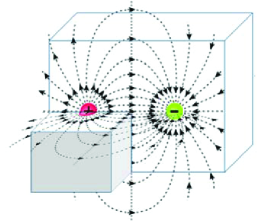
Figure 1: Electric field lines for two interacting particles in a uniform dielectric environment in 3D materials.

II.2 2D excitons

Since the experimental discovery of highly conductive graphene monolayers in 2004 Novoselov , the field of condensed matter physics has seen explosive growth in theoretical and experimental research in the realm of two-dimensional materials. The isolation of graphene from bulk crystals of graphite allowed the identification of just the first member of a family of 2D layered materials, which has grown rapidly over the past ten years and now includes insulators, semiconductors, semimetals, metals, and superconductors Bhimanapati ; Novoselov2 . 2D materials are commonly defined as crystalline materials consisting of a single layer of atoms. Most often such materials are classified as either 2D allotropes of various elements or compounds consisting of two or more ionically/covalently bonded elements. 2D materials have, within just one decade, reshaped many disciplines of modern science, both through intensive experimental and theoretical studies of their properties, as well as by providing a rich platform for further exploration of previously-known and newly-emerging exotic physical phenomena. These materials are crystalline solids with a high ratio between their lateral size and thickness Velicky . In these layered materials, known also as van der Waals materials, the atomic organization and bond strength in the 2D plane are typically much stronger than in the third dimension (out-of-plane), where they are bonded together by weak van der Waals’ interaction Novoselov2 ; Jariwala . Today, research in the field is primarily focused on graphene, transition metal dichalcogenides (TMDCs) and other emerging 2D materials beyond graphene such as phosphorene and transition metal trichalcogenides (TMTCs), which are the anisotropic semiconductors, and Xenes. These nanomaterials are essential for the next generation of devices in tunable optoelectronics, sensing, and photovoltaics. The gapless nature of graphene makes it less ideal for the study of optical phenomena in 2D crystals Novoselov3 . In terms of materials, the most well studied 2D materials beyond graphene are the semiconducting transition metal dichalcogenides with the chemical formula MX₂, where M denotes a transition metal M = Mo, W, and X denotes a chalcogenide X = S, Se, or Te Kormanyos , transition metal trichalcogenides Joshua and phosphorene Li1 ; Li2 ; Warren2015 . In recent years, experimental success was achieved in isolating stable monolayers of 2D insulators such as hexagonal boron nitride (h-BN) Dean2010 . It is often the case that any study of 2D materials includes the use of h-BN as a substrate or spacer.

Another recent addition to the 2D universe are the buckled 2D materials Matthes2014 collectively referred to as Xenes Molle2017 ; Brunetti2018 : silicene (Si) Falko2012 , germanene (Ge) Davila , stanene (Sn) Zhu2014 , and borophene (B) Mannix2015 . In the buckled 2D materials, the triangular sublattices of the honeycomb structure are vertically offset from each other by an amount which is small compared to the 2D bond length. These direct band gap materials exhibit a Dirac cone near the K/K^′ points, but have a non-zero gap with a parabolic dispersion in the immediate vicinity of the K/K^′ points, making them an intriguing counterpart to gapless graphene. Most interestingly, the vertical offset between the sublattices means that the band-gap can be tuned by applying an external electric field, leading to, among other things, a large and externally tunable exciton binding energy. In Fig. 2, we schematically illustrate an incomplete zoo of some of the important members of this 2D family.

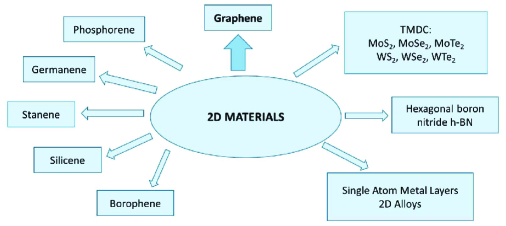
Figure 2: Schematic of a zoo of some of the important members of the 2D family.

New 2D materials offer reasonable flexibility in terms of tailoring their electronic and optical properties. The emergence of each new material brings excitement and puzzlement towards their characterization and physical properties, while expanding the tool set with which scientists may combine these materials in novel and useful ways. Together, the zoo of 2D materials offers a truly unique and exciting platform for creating novel heterostructures with unique properties by stacking the aforementioned 2D materials in different ways, which the authors of Ref. Geim2014 notably described as analogous to building with lego bricks. The properties of these materials are usually distinctly different from those of their 3D counterparts, and furthermore, the properties of these materials can drastically change even when transition from a single, isolated monolayer to two monolayers separated by a dielectric. An important characteristic of the 2D materials is the weak and highly non-local way in which they screen electric fields Rytova ; Keldysh .

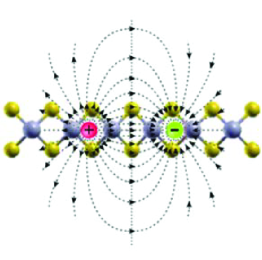
Figure 3: Electric field lines for two interacting particles in 2D materials.

The reduction of dimensionality has a strong influence on a two-body system and its effect is twofold: it decreases the kinetic energy and potential energy of interacting charge carriers. In the two-body problems if the interaction is described by the Coulomb potential and the dielectric environment is homogenous, but the electron and hole are constrained to move in a plane, the reduction of dimensionality affects only the kinetic energy of the system and one can observe that the spectrum of energy is changed from $E_{3D}\sim 2\varepsilon\hslash^{2}/n^{2}$ ($n=1,2,...,$ Rydberg series) in the 3D case, to $E_{2D}\sim 2\varepsilon\hslash^{2}/(n-1/2)^{2}$ in the 2D case. Therefore, for example, the ground state energy increases by a factor of 4. Thus, the reduction of dimensionality suppresses the kinetic energy of the 2D exciton due to the decrease of the degrees of freedom. However, the reduction of the dimensionality affects on the potential energy of the electron-hole interaction, while this interaction is still electromagnetic by nature, it must be modified from the well-known Coulomb potential. As mentioned above, in 3D the screening is given by a simple multiplicative renormalization by the dielectric constant $\varepsilon$ due to the homogeneous dielectric environment. In contrast to the 3D case, in 2D case the system is polarizable only in the 2D plane and the induced polarization field is equivalent to the electric field produced by a uniform charge distribution on a circle of radius $r$, in contrast to the uniform charge distribution on the sphere of radius $r$ in case of a 3D material. Therefore, in comparison to the 3D case shown in Fig. 1, the electric field outside of the 2D plane shown in Fig. 3 does not affect on two particle interaction, unlike the portion of the electric field lying within the 2D monolayer. As a consequence this interaction still will be a function of $r$, but with a functional form substantially different from the Coulomb potential. The 2D electromagnetic interaction between two point charges in a layered dielectric environment was first derived in Ref. Rytova , was independently re-derived over a decade later in Ref. Keldysh , and is now known as the Rytova-Keldysh (RK) potential. This interaction has the following form:

$$V(r_{eh})=-\frac{\pi ke^{2}}{\left(\varepsilon_{1}+\varepsilon_{2}\right)\rho_{0}}\left[H_{0}\left(\frac{r}{\rho_{0}}\right)-Y_{0}\left(\frac{r}{\rho_{0}}\right)\right].$$ (1)

In Eq. (1) $r$ is the distance between the electron and hole, $k\equiv 1/(4\pi\epsilon_{0})=9\times 10^{9}\$N$\cdot$m²/C², $H_{0}(x)$ and $Y_{0}(x)$ are Struve and Bessel functions of the second kind of order $\nu=0$, respectively, $\varepsilon_{1}$ and $\varepsilon_{2}$ denote the background dielectric constants on either side of the monolayer, and the screening length $\rho_{0},$ which sets the boundary between the two distinct asymptotic behaviors of the RK potential for $r\dashrightarrow 0$ and $r\dashrightarrow\infty$, is defined by $\rho_{0}=2\pi\zeta/\left[\left(\varepsilon_{1}+\varepsilon_{2}\right)/2\right]$, where $\zeta\$is the 2D polarizability of the material. For $r>>\rho_{0}$ the potential has the 3D bare Coulomb tail and becomes $-\frac{ke^{2}}{\varepsilon r}$, while for $r<<\rho_{0}$ it becomes a logarithmic potential: $-\frac{ke^{2}}{\varepsilon\rho_{0\text{ }}}\left[\ln\left(\frac{r}{2\rho_{0}}\right)+\gamma\right],$ where $\gamma$ is the Euler constant. Thus at small distance the effect of the induced polarization becomes dominant - the $1/r$ singularity is replaced by a weaker logarithmic dependence. The recent review of dynamical screening in monolayer transition-metal dichalcogenides is given in Ref. Dery2019 .

The exciton can be formed in a double layer system when an electron is confined in one layer, while the hole is located in a parallel layer separated by a dielectric of a thickness $D.$ Such excitons with spatially separated electrons and holes are known as indirect or dipolar excitons, and were first introduced in Ref. Nishanov . In this system the excitons can have a much longer lifetime than the direct excitons MoskalenkoSnoke , because the dielectric barrier between the layers reduces the probability of electron-hole recombination by tunneling. The prediction of superfluidity and Bose-Einstein condensation  Lozovik of indirect excitons in semiconductor coupled layers attracted a great interest to this system Snoke ; Butov ; Combescot . The theoretical description of an indirect exciton is a two-body problem in restricted 3D space when electron and hole can move each in one of the layers, while motion in the third direction is restricted by the layers separation $D$. To solve this problem one projects the electron position vector onto the plane with the hole and the relative position vector between the electron and the hole is $\mathbf{r}_{e}-\mathbf{r}_{h}=\mathbf{r}+D\widehat{\mathbf{z}}$, where $\widehat{\mathbf{z}}$ is unit vectors, $D$ is the fixed interlayer separation, and $\mathbf{r}$ is the separation between the hole and the projection of the electron position onto the TMDC layer with holes. One can replace the relative coordinate by $\sqrt{r^{2}+D^{2}}$ and, as a consequence, the electron-hole potential should be replaced by

$$V(r)=-\frac{\pi ke^{2}}{\left(\varepsilon_{1}+\varepsilon_{2}\right)\rho_{0}}\left[H_{0}\left(\frac{\sqrt{r^{2}+D^{2}}}{\rho_{0}}\right)-Y_{0}\left(\frac{\sqrt{r^{2}+D^{2}}}{\rho_{0}}\right)\right]\text{ \ or \ }V(r)=-\frac{ke^{2}}{\varepsilon\sqrt{r^{2}+D^{2}}}.$$ (2)

for the RK or Coulomb electron$-$hole interaction, respectively. Recently electrostatic interactions in a bilayer system of TMDC material, which is a generalization of the RK potential was suggested in Ref. Hunt2018 .

It is reasonable in a double layer system when the separation between layers is big enough to consider the oscillatory approximation (OA) for the RK, as well as the Coulomb potentials BermanKezerashviliFBS2011 ; RKPhysRevB2012 ; RKPhysRevB2016 ; RKPhysRevB2017 . Assuming that $r\ll D$, one can expand Eq. (2) as a Taylor series in terms of $\left(r/D\right)^{2}$. By limiting ourselves to the first order with respect to $\left(r/D\right)^{2}$, we obtain

$$V(r)=-V_{0}+\beta r^{2},$$ (3)

where

$$V_{0} = \frac{\pi ke^{2}}{\left(\varepsilon_{1}+\varepsilon_{2}\right)\rho_{0}}\left[H_{0}\left(\frac{D}{\rho_{0}}\right)-Y_{0}\left(\frac{D}{\rho_{0}}\right)\right],\text{ }\beta=-\frac{\pi ke^{2}}{2\left(\varepsilon_{1}+\varepsilon_{2}\right)\rho_{0}^{2}D}\left[H_{-1}\left(\frac{D}{\rho_{0}}\right)-Y_{-1}\left(\frac{D}{\rho_{0}}\right)\right];$$ (4)

$$V_{0} = \frac{ke^{2}}{\varepsilon D},\text{ \ }\beta=\frac{ke^{2}}{2\varepsilon D^{3}}.$$ (5)

Eqs. (4) and (5) define parameters $V_{0}$ and $\beta$ for the oscillatory approximation of the RK and Coulomb potentials, respectively, and $H_{-1}\left(\frac{D}{\rho_{0}}\right)$ and $Y_{-1}\left(\frac{D}{\rho_{0}}\right)$ are Struve and Bessel functions of the second kind of order $\nu=-1$, correspondingly.

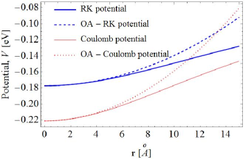
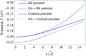
Figure 4: The comparison of the RK and Coulomb potentials and their oscillatory approximations for the electron-hole interaction in MoSe₂ (a) and phosphorene (b) double layer. At $r<6$ Å the oscillatory approximation (3) is a good approximation for both the RK and Coulomb potentials. At $r>10$ Å the RK and Coulomb potentials converge each other as $r$ increases.

Comparisons of the RK and Coulomb potentials for an electron-hole pair in a MoSe₂ and phosphorene double layer, as well as their oscillatory approximation are shown in Fig. 4. According to Fig. 4, the RK potential is weaker than the Coulomb potential at small projections $r$ of the electron-hole distance on the monolayer plane, while both potentials converge to each other as $r$ increases. The electron-hole attraction potentials for a MoSe₂ double layer are significantly larger than for a phosphorene double layer. The difference between the Rytova-Keldysh and Coulomb potentials for the phosphorene double layer is much larger than for the MoSe₂ double layer, while the Coulomb potentials for both materials must be the same. In Fig. 4 is considered the case when two monolayers are separated by 4 h-BN monolayers, corresponding to $D=1.332\ \mathrm{nm}$.

In the low-energy limit, low-energy excitations (e.g. electrons and holes) in gapless graphene electrons and holes behave as relativistic massless particles described by the Weyl equation for massless and chiral particles Guinea ; Vozmediano , while in gapped 2D materials, excitons are described by a Dirac-like equation Kormanyos ; Xiao ; Tabert . Therefore, the physics around the K and K^′ points has attracted the most attention both experimentally and theoretically. The two-band single electron Hamiltonian in the $k\cdot p$ approximation in the vicinity of the K/K^′ points was introduced in Ref. Xiao for TMDCs and Ref. Tabert for a buckled honeycomb lattice in the presence of a perpendicular electric field and are given respectively as

$$H = at\left(\xi k_{x}\hat{\sigma}_{x}+k_{y}\hat{\sigma}_{y}\right)+\frac{\Delta}{2}\hat{\sigma}_{z}-\lambda\xi\frac{\hat{\sigma}_{z}-1}{2}\hat{s}_{z},$$ (6)

$$H = \hbar v_{F}(\xi k_{x}\hat{\tau}_{x}+k_{y}\hat{\tau}_{y})-\xi\Delta_{so}\hat{\sigma}_{z}\tau_{z}+\Delta_{z}\tau_{z}.$$ (7)

In Eqs. (6) and (7) $\hat{\tau}$ and $\hat{\sigma}$ are the Pauli matrices for the spin and pseudospin, respectively, $k_{x}$ and $k_{y}$ are the components of momentum in the $xy$-plane of the monolayer, relative to the K and K^′ points, $\xi=1$ ($\xi=-1)$ is the valley index and denotes the valley K (K^′), $2\lambda$ is the spin splitting at the valence band caused by spin-orbit coupling in TMDCs, while in the Xenes, $2\Delta_{so}$ is the intrinsic gap between the conduction and valence bands at zero electric field, and is also the splitting due to spin-orbit coupling between the two conduction or two valence bands at large electric fields. Let us also mention that in (6) $a$ is the lattice constant, $t$ is the effective hopping integral (these parameters for a set of the most common layered transition metal dichalcogenides $\mathrm{MoS_{2}}$, $\mathrm{MoSe_{2}}$, $\mathrm{MoTe_{2},}$ $\mathrm{WS_{2}}$, $\mathrm{WSe_{2}}$ and $\mathrm{WTe_{2}}$ are listed in Refs. Kormanyos ; Xiao ), $\Delta$ is the energy gap, $\hat{s}_{z}$ is the Pauli matrix for spin that remains a good quantum number, while in Eq. (7) $\Delta_{z}=ed_{0}E_{\perp}$ is the gap induced by the electric field, $E_{\perp},$ normal to a monolayer, where $d_{0}$ in the latter expression is the buckling constant Tabert . The first term in Eq. (7) is the same as that of the low-energy Hamiltonian in graphene Guinea ; Vozmediano . The second term in (6) present the energy gap in TMDC, while for the Xenes in (7) the second term describes the intrinsic band gap and the third term gives the modification of the band gap due to the external electric field. One should emphasize that in Eq. (7) as well as in the Weyl’s type equation for the gapless graphene $v_{F}$ is the Fermi velocity, in contrast to speed of light in the Weyl and Dirac equations. Therefore, the Hamiltonians (6) and (7), as well as the Hamiltonians for the gapped and gapless graphene are not relativistically invariant.

Excitons in monolayers and in heterostructures of these monolayers are usually treated using one of two theoretical methods: the standard quantum mechanical approach, where the Schrödinger equation for an interacting electron and hole is solved in the framework of the effective mass approximation, and as a ”quasirelativistic” system of two coupled Dirac particles. The first approach, involving separation of the center-of-mass and relative coordinates, with a scalar interparticle potential, is completely understood and is well-developed in configuration and momentum space in 3D as well as 2D Landau ; Liboff ; Griffiths . By contrast, the description of the relativistic two-body problem is much more complicated and until now no completely self-consistent formalism for the separation of center-of-mass and relative coordinates has been developed, even for the two-body case. This is due to the following facts stemming from the relativistic treatment of the electron and hole RKPhysRevA2012 :

i) the particles’ locations and momenta are 4-vectors;

ii) the momenta are not independent but must satisfy mass-shell conditions;

iii) the inter-particle interaction potentials appear in the boosts as well as in the energy generator in the instant form of dynamics. As a result of a transformation to the center-of-mass system, even a scalar inter-particle potential becomes dependent on both a coordinate and momentum;

iv) the structure of the Poincare’ group implies that there is no definition of relativistic 4-center of mass sharing all the properties of the non-relativistic 3-center of mass Alba .

The two-body problem in condensed matter physics for the electron and hole with the Hamiltonians (6) and (7) becomes even more complicated than in the simple relativistic case. It is related to the following: i) resultant equations from the Hamiltonians (6) and (7) become non-covariant and canonical transformation implementing the separation of the center-of-mass from the relative variables within relativistic approach is invalidated; ii) even though the electron-hole interaction in the RK or Coulomb potentials depends only on the coordinate of the relative motion, after the center-of-mass transformation the potential acquires a dependence on the momenta and also due to the chiral nature of charge carriers one cannot separate the center-of-mass and relative motions.

Based on the single-particle Hamiltonians (6) and (7) one can write the Hamiltonian for the interacting electron-hole system. The general form of this Hamiltonian in the vicinity of the $K/K^{\prime}$ points for direct or indirect excitons formed by spin-up (spin-down) particles is the following:

$$\mathcal{H}_{\uparrow(\downarrow)}=\left(\begin{array}[]{cccc}V(r)&\partial_{2}&\partial_{1}&0\\ \partial_{2}^{\dagger}&-\Delta^{\prime}+V(r)&0&\partial_{1}\\ \partial_{1}^{\dagger}&0&\Delta^{\prime}+V(r)&\partial_{2}\\ 0&\partial_{1}^{\dagger}&\partial_{2}^{\dagger}&V(r)\end{array}\right)\ ,$$ (8)

where $V(r)$ is the potential energy of the attraction between an electron and a hole, which is given by Eq. (1) or by the Coulomb potential in the case of direct excitons or by Eqs. (2) in the case of indirect excitons. In Eq. (8) the parameter $\Delta^{\prime}$ is defined as $\Delta^{\prime}=\Delta-\lambda$ ($\Delta^{\prime}=-2\Delta_{z}+2\Delta_{so})$ for spin-up particles, and $\Delta^{\prime}=\Delta+\lambda$ ($\Delta^{\prime}=2\Delta_{z}-2\Delta_{so})$ for spin-down particles for TMDCs (Xenes). In Eq. (8) $\partial_{1}=C(-i\partial_{x_{1}}-\partial_{y_{1}})$, $\partial_{2}=C(-i\partial_{x_{2}}-\partial_{y_{2}})$ and the corresponding Hermitian conjugates are $\partial_{1}^{\dagger}=C(-i\partial_{x_{1}}+\partial_{y_{1}})$, $\partial_{2}^{\dagger}=C(-i\partial_{x_{2}}+\partial_{y_{2}})$, where $C$ is a constant and $C=at$ for the TMDC and $C=\hbar v_{F}$ for the Xenes and graphene. Operators are defined as $\partial_{x}=\partial/\partial x$ and $\partial_{y}=\partial/\partial y,$ when $x_{1}$, $y_{1}$ and $x_{2}$, $y_{2}$ are the coordinates of vectors $\mathbf{r}_{1}$ and $\mathbf{r}_{2}$ for an electron and hole, correspondingly.

The Hamiltonian (8) describes two interacting particles located in 2D monolayers or 2D double layers and satisfies the following conditions:

i) when the potential $V(r)=0$, the Hamiltonian describes two non-interacting Dirac particles in mono or double layers.

ii) when $\Delta^{\prime}=0$ and $V(r)$ is the Coulomb potential, the Hamiltonian describes two interacting Dirac particles in gapless graphene and is identical to the Hamiltonian Sabio representing the two-body problem in gapless graphene layer;

iii) depending on the values of $\Delta^{\prime}$ the Hamiltonian (8) describes the interacting the electron-hole system via the RK potential Keldysh in a monolayer TMDC or Xenes. In the case of indirect excitons, when the electron and hole are located in two different monolayers with the interlayer separation $D$, one can consider the electron-hole interaction via the RK or Coulomb potentials (2) or use the OA (3).

The energy spectrum of an electron-hole pair can be found by solving the eigenvalue problem for the Hamiltonian (8):

$$\mathcal{H}_{\uparrow(\downarrow)}\Psi_{\uparrow(\downarrow)}=\epsilon_{\uparrow(\downarrow)}\Psi_{\uparrow(\downarrow)}\ ,$$ (9)

where $\epsilon_{\uparrow(\downarrow)}$ is the energy spectrum for an electron-hole pair with the up and down spin orientation. The eigenfunction $\Psi_{\uparrow(\downarrow)}$ in Eq. (8) is four-component spinor, where the spinor components refer to the four possible values of the conduction/valence band indices and is given as:

$$\Psi_{\uparrow}(\mathbf{r}_{1},\mathbf{r}_{2})=\left({\begin{array}[]{c}\phi_{c\uparrow c\uparrow}(\mathbf{r}_{1},\mathbf{r}_{2})\\ \phi_{c\uparrow v\uparrow}(\mathbf{r}_{1},\mathbf{r}_{2})\\ \phi_{v\uparrow c\uparrow}(\mathbf{r}_{1},\mathbf{r}_{2})\\ \phi_{v\uparrow v\uparrow}(\mathbf{r}_{1},\mathbf{r}_{2})\end{array}}\right)\equiv\left({\begin{array}[]{c}\Psi_{c\uparrow}\\ \Psi_{v\uparrow}\end{array}}\right),\text{ where }\Psi_{c\uparrow}=\left({\begin{array}[]{c}\phi_{c\uparrow c\uparrow}\\ \phi_{c\uparrow v\uparrow}\end{array}}\right),\ \ \ \Psi_{v\uparrow}=\left({\begin{array}[]{c}\phi_{v\uparrow c\uparrow}\\ \phi_{v\uparrow v\uparrow}\end{array}}\right),$$ (10)

where a quasiparticle is characterized by the coordinates $\mathbf{r}_{j}$ in the conduction ($c$) and valence ($v$) band with the corresponding direction of spin up $\uparrow$ or down $\downarrow$, and index $j=1,2$ referring to the two monolayers, one with electrons and the other with holes. In this notation we assume that a spin-up (-down) hole describes the absence of a spin-down (-up) valence electron. The two components reflect one particle being in the conduction (valence) band and the other particle being in the valence (conduction) band, correspondingly. Let us mention that while (10) represents the spin-up particles, the spin-down particles are represented by the same expression replacing $\uparrow$ by $\downarrow$.

As aforementioned, for the Hamiltonian (8) the center-of-mass motion cannot be separated from the relative motion in the quasirelativistic approach due the chiral nature of charge carriers in 2D materials. A similar conclusion was made for the two-particle problem in graphene  Sabio , gapped graphene RKPhysRevB2012 and TMDC monolayers RKPhysRevB2016 . Since the RK and Coulomb interactions depend only on the relative coordinate of the electron-hole system, one can introduce the “center-of-mass” coordinate and the relative motion coordinate in the plane of a monolayer: $\mathbf{R}=\alpha\mathbf{r}_{1}+\delta\mathbf{r}_{2},\mathbf{r}=\mathbf{r}_{1}-\mathbf{r}_{2}$, where the coefficients $\alpha$ and $\delta$ are supposed to be found for a small momentum $\mathbf{K}$ from the condition of the separation of the coordinates of the center-of-mass and relative motion of an electron-hole in the one-dimensional equation for the corresponding components of the spinor $\Psi_{\uparrow(\downarrow)}$ RKPhysRevA2012 . One can obtain the solution of Eq. (9) by making the following Anzätze

$$\Psi_{j\uparrow(\downarrow)}(\mathbf{R},\mathbf{r})=\mathtt{e}^{i\mathbf{K}\cdot\mathbf{R}}\psi_{j\uparrow(\downarrow)}(\mathbf{r})\ ,$$

and follow the procedure given in Refs. RKPhysRevA2012 ; RKPhysRevB2012 ; RKPhysRevB2016 one derives an equation for the components $\phi_{c\uparrow(\downarrow)v\uparrow(\downarrow)}$ of the spinor $\Psi_{\uparrow(\downarrow)}.$ As an example, let us introduce the equation for the components $\phi_{c\uparrow(\downarrow)v\uparrow(\downarrow)}$ of the bound electron-hole system for TMDC materials RKPhysRevB2016 :

$$\left(-F_{1}(\epsilon_{\uparrow(\downarrow)})\nabla_{\mathbf{r}}^{2}+V(r)\right)\phi_{c\uparrow(\downarrow)v\uparrow(\downarrow)}=F_{0}^{\prime}(\epsilon_{\uparrow(\downarrow)})\phi_{c\uparrow(\downarrow)v\uparrow(\downarrow)}\ ,$$ (11)

where

$$F_{1}(\epsilon_{\uparrow(\downarrow)})=\frac{2a^{2}t^{2}}{\epsilon_{\uparrow(\downarrow)}}\ ,\text{ \ \ \ \ \ }F_{0}^{\prime}(\epsilon_{\uparrow(\downarrow)})=\epsilon_{\uparrow(\downarrow)}+\Delta^{\prime}-\frac{a^{2}t^{2}\mathcal{K}^{2}}{2\epsilon_{\uparrow(\downarrow)}}\ .$$ (12)

II.2.1
Double layers of TMDC

For the two-body electron-hole system interacting via the Rytova-Keldysh potential, Eq. (11) has no analytical solution and can only be solved numerically, while for the Coulomb potential one can obtain an analytical solution RKPhysRevA2012 . For indirect excitons, (11) can be solved only numerically for both types of potentials. One can consider a spatially separated electron-hole pair in two parallel TMDC layers at large distances $D\gg a_{B}$, where $a_{B}$ is the 2D Bohr radius of a dipolar exciton and use the oscillatory approximation (3). For TMDC materials the Bohr radius of the dipolar exciton is found to be in the range from $1.5\ \mathrm{{\mathring{A}}}$ for $\mathrm{MoTe_{2}}$ Ashwin up to $3.9\ \mathrm{{\mathring{A}}}$ for $\mathrm{MoS_{2}}$ Louie . Therefore, one can use the OA (3), which allows one to reduce the problem of indirect exciton to an exactly solvable two-body problem. By substituting (3) into Eq. (11), one obtains an equation that has the form of the Schrödinger equation for the 2D isotropic harmonic oscillator:

$$\left(-F_{1}(\epsilon_{\uparrow(\downarrow)})\nabla_{\mathbf{r}}^{2}+\beta r^{2}\right)\phi_{c\uparrow(\downarrow)v\uparrow(\downarrow)}=F_{0}(\epsilon_{\uparrow(\downarrow)})\phi_{c\uparrow(\downarrow)v\uparrow(\downarrow)}\ ,$$ (13)

where $F_{0}(\epsilon_{\uparrow(\downarrow)})=F_{0}^{\prime}(\epsilon_{\uparrow(\downarrow)})+V_{0},$ and parameters $V_{0}$ and $\beta$ are given by Eqs. (4) and (5) for  both the Rytova-Keldysh and Coulomb potentials, respectively.

The solution of the Schrödinger equation for the harmonic oscillator, is well known and is given by

$$\frac{F_{0}(\epsilon_{\uparrow(\downarrow)})}{F_{1}(\epsilon_{\uparrow(\downarrow)})}=2N\sqrt{\frac{\beta}{F_{1}(\epsilon_{\uparrow(\downarrow)})}}\ ,$$ (14)

where $N=2\tilde{N}+|L|+1$, and $\tilde{N}=\mathrm{min}(\widetilde{n},\widetilde{n}^{\prime})$, $L=\widetilde{n}-\widetilde{n}^{\prime}$, $\widetilde{n},$ $\widetilde{n}^{\prime}=0,1,2,3,\ldots$ are the quantum numbers of the 2D harmonic oscillator. The corresponding 2D wave function can be expressed in terms of associated Laguerre polynomials RKPhysRevB2016 .  Thus, considering Eq. (11) for indirect excitons and using the oscillatory approximation, we can reduce the problem of indirect exciton to an exactly solvable two-body problem. The binding energy for the indirect exciton was estimated for two $\mathrm{MoS_{2}}$ layers separated by $N$ h-BN insulating layers from $N=1$ up to $N=6$ Fogler . These dipolar excitons were observed experimentally for $N=2$ Calman . We assume that the indirect excitons in TMDCs can survive for a larger interlayer separation $D$ than in semiconductor coupled quantum wells, because the thickness of a TMDC layer is fixed, while the spatial fluctuations of the thickness of the semiconductor quantum well affects the stability of the dipolar exciton. The theoretical analysis presented above is quite general and can be applied to any TMDC monolayer or a double layer system with two different Mo- and W-based monolayers. The effect of different dielectric environments on the exciton binding energy in the framework of a four-band Hamiltonian describing indirect excitons is investigated and a remarkable dependence on the dielectric constant of the barrier between the two layers is found Peeters2018 .

The description of the Mott-Wannier excitons within the effective mass potential model requires two main inputs of material-specific ingredients such as electrons and holes effective masses, which are easily calculated from ab initio band structures, and polarizability of the monolayer, which is an essential parameter for the description of the screened electron-hole interaction. The screening effects are negligible for electron-hole distances larger than the screening length $\rho_{0}$, and at long range the electron-hole interaction is described by the Coulomb potential Reichman2013 . The screening length is defined by the 2D polarizability of the planar material Rubio . Using the polarizabilities from Ref. Reichman2013 , we conclude that $\rho_{0}$ is estimated as $38\ \mathrm{{\mathring{A}}}$ for $\mathrm{WS_{2}}$, $41\ \mathrm{{\mathring{A}}}$ for $\mathrm{MoS_{2}}$, $45\ \mathrm{{\mathring{A}}}$ for $\mathrm{WSe_{2}}$, $52\ \mathrm{{\mathring{A}}}$ for $\mathrm{MoSe_{2}}$. The spin-orbit coupling in TMDC monolayers leads to a spin-orbit splitting in the valence band and to the formation of two distinct types $A$ and $B$ excitons Reichman2013 ; Kormanyos . $A$ excitons are formed by spin-up electrons from conduction and spin-down holes from valence band, while type $B$ excitons are formed by spin-down electrons from conduction and spin-up holes from valence band GlazovRMP . Comparing the binding energies of excitons over different TMDC layers, one can observe that the binding energy depends weakly on the effective masses, but strongly on the material polarizability. As a consequence, the binding energy for $A$ and $B$ excitons, which have different effective masses are generally very similar in the same monolayer DenFuncTheoryPIMC ; BrunettiJP2018 .

II.2.2 Phosphorene

The exciton binding energy of monolayer phosphorene on a SiO₂/Si substrate was determined to be $\sim$0.9 eV WangPhosphorenEx . This result agrees well with the theoretical prediction that substrate screening strongly affects the exciton binding energy in monolayer phosphorene Rodin . A theoretical study of the exciton binding energy using the screened electron-hole interaction for anisotropic two-dimensional crystals is presented in Ref. Prada , where the authors obtained analytical expressions using variational wave functions in different limits of the screening length. The analytical solution for the exciton binding energy using the variational approach Prada gives a result which compares well with the numerical one and is in reasonable agreement with the experimental value for the monolayer of black phosphorous. A recent ab initio study Hunt22019 has used the diffusion Monte Carlo method to study the exciton binding energy of monolayer phosphorene from first-principles. The double layer phosphorene system with a number of h-BN monolayers, placed between two phosphorene monolayers was investigated in Ref. RKPhysRevBG2017 . The different lattice constants from the literature in turn causes the difference in the band curvatures, and, therefore, in the different effective masses of charge carriers. The binding energies of indirect excitons formed in the double layer phosphorene with 7 h-BN monolayers, calculated for the sets of the different masses corresponding to the different lattice constants are 28.2 meV, 29.6 meV, 37.6 meV, and 37.2 meV RKPhysRevBG2017 .

II.2.3 Xenes

Related to the 2D Xenes, the study of binding energies and optical properties of direct and indirect excitons in monolayers and double layer heterostructures of Xenes (silicene, germanene, and stanene) is presented in Ref. Brunetti2018 , where the Schrödinger equation with electric field-dependent exciton reduced mass is solved by using the RK potential for direct excitons, while both the RK and Coulomb potentials are used for indirect excitons.  One of the important features of the 2D semiconductors is the existence of strongly bound excitons with binding energies reaching up to 30% of the band gap. However, calculations of the binding energies with the RK potential as a function of external electric field in freestanding Xenes Brunetti2019  demonstrate that these binding energies are far larger than their respective band gaps, when the electric field is small or zero. This phenomena could be an indicator of the excitonic insulating phase in these materials. Thus, one can observe a phase transition in monolayer Xenes from the excitonic insulator ground state to the semiconducting phase by increasing the electric field beyond some critical value which is unique to each material. In the case of an Xene monolayer on a substrate, the enhanced dielectric screening from the substrate reduces the exciton binding energy such that Xenes on a substrate should not exhibit the excitonic insulator phase.

II.3 1D excitons

To model the electrostatic interaction of an electron and hole in 1D quantum system, Poisson’s equation is first solved to find the electrostatic potential of a point-like charge $e$ inside a 1D structure, which is considered as a dielectric cylinder. The cumbersome nature of such a potential makes it impossible to solve two-body problem analytically. However, it can be solved when the complicated potential is approximated by an effective potential. One first calculates the 1D subband energies and wave functions, while neglecting the Coulomb interaction, and using these wave functions of transverse electron and hole motion, calculates the longitudinal motion of the exciton, including corrections from image forces in the surrounding medium. To do that, the three dimensional Coulomb potential is averaged to a one dimensional Coulomb interaction between the electron and hole along the 1D nanostructure axis Bartnik ; Giblin . Thus, to perform the calculations, the Coulomb potential is often replaced by approximate model potentials. There are different models of the effective interaction potential: i. The effective 1D electron-hole interaction is modeled as cusp-type Coulomb potential $V(z)=-\frac{ke^{2}}{4\pi\varepsilon_{0}\varepsilon}\frac{A}{z-r_{0}}$, where the parameters $A$ and $r_{0}$ are determined self-consistently by employing the eigenfunctions of the lateral confinement of electrons and holes OgawaTakagahara ; RK1D ; ii. The singularity of the Coulomb potential is cut off at $r=a$, where $a$ is the radius of the wire, and the effective potential is $V(z)=-\frac{ke^{2}}{4\pi\varepsilon_{0}\varepsilon}\frac{1}{\sqrt{z^{2}+a^{2}}}$ DasSarma ; Semina ; iii. An assumption of strong lateral confinement, allows separation of the $z$ motion from the lateral motion in the $xy$ plane, and by averaging the 3D Coulomb interaction potential over the transverse degrees of freedom, an analytical 1D formula for the effective interaction potential between the confined charge carriers is derived Bednarek2003 ; Slachmuylders . iv. The potential is divided into four terms: the unscreened direct interaction of the two charges, the modification of this interaction due to the image effects, and the two self-interactions of each charge with its own image, and the adiabatic potential is obtained by averaging the potential over wave functions of the corresponding electron and hole subband Bartnik . However, in all cases the electromagnetic interaction between the charge carriers is not given by the 3D Coulomb potential but rather by one-dimensional potentials, which have a Coulomb tail, and consequently the highly excited bound eigenstates of 1D excitons have a Rydberg series structure. Calculations show that for charge carriers confined in 1D nanostructures, the aforementioned effective 1D model potentials work with a reasonable precision in a wide range of nanostructure parameters. Fig. 5 depicts the electric field lines between the interacting electron and hole. For 2D materials, field lines are screened along the plane and mainly lie unscreened in the vacuum. In 1D materials, field lines lie mainly in the vacuum, hence screening is heavily suppressed.

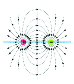
Figure 5: Electric field lines for two interacting particles in 1D materials.

Following OgawaTakagahara one can write the equation that describes one-dimensional relative motion of the electron and hole interacting via a cusp-type Coulomb interaction as

$$-\frac{\hbar^{2}}{2\mu}\frac{d^{2}\Phi_{X}(z)}{dz^{2}}-\frac{A_{eh}}{\left|z\right|+Z_{0eh}}\Phi_{X}(z)=E_{X}\Phi_{X}(z).$$ (15)

Here $\mu$ is the reduced effective mass of the electron-hole pair, $A_{eh},$ $Z_{0eh}$ are the fitting parameters for the effective electron$-$hole one-dimensional cusp-type Coulomb potentials obtained through the parametrization, $z=z_{e}-z_{h}$ is the relative electron-hole motion coordinate, $-E_{X}$ is the binding energy of the exciton, and $\Phi_{X}(z)$ is the corresponding excitonic eigenfunction. Eq. (15) has the same form as the equation for one-dimensional hydrogen atom studied by Loudon Loudon1 . One can introduce the following notations

$$\xi^{2}=-\frac{\hbar^{2}\eta_{0}^{2}}{2\mu E_{X}},\text{ }\eta_{0}=\frac{A_{eh}\mu}{\hbar^{2}},\text{ }x=\frac{2\eta_{0}(\left|z\right|+Z_{eh})}{\xi}$$ (16)

and reduce (15) to the Whittaker’s equation

$$\frac{d^{2}\zeta(x)}{dx^{2}}+\left(-\frac{1}{4}+\frac{\xi}{x}\right)\zeta(x)=0.$$ (17)

The solution of (17) is $\zeta(x)=W_{\xi,\pm 1/2}(x)$ Loudon1 ; Loudon2 ; Loudon3 , where $W_{\xi,\pm 1/2}(x)$ is the Whittaker function. The value of $\xi$ which defines $E_{X}$ and $\Phi_{X}(z)$, is determined by the boundary condition stating that for even states the derivative of wavefunction at $z=0$ must turn to zero

$$\frac{d}{dz}\left[W_{\xi,\pm 1/2}\left(\frac{2\eta_{0}(\left|z\right|+Z_{eh})}{\xi}\right)\right]_{z=0}=0.$$ (18)

The full Hamiltonian of excitons in a quantum nanowires (NWR) is constructed within $k\cdot p$ theory using the single-band effective mass approximation or even four-band effective mass model Bartnik . The formation, stability, and binding energy of excitons depends on the electron to hole mass ratio and the geometric characteristics of a nanostructure, such as the shape of the NWR, the radius of the NWR or carbon nanotudes (CNT), and the thickness of a shell for core/shell NWR. The excitons in NWRs and CNTs are well studied objects and theoretical calculations have shown that the effective 1D interaction leads to accurate results for different characteristics of NWRs as well as CNTs, which are in reasonable agreement with available experimental data.

III Three Body Problem$-$Trions

In the late 1950s Lampert L predicted the existence of charged three-particle complexes: a negatively (X^-) and positively (X⁺) charged trions, formed when an electron in a conduction band or a hole in a valence band is bound to an exciton. This idea gave rise to many publications in the 60s and the 70s to study trions in bulk materials. The binding energies of these exciton complexes are very small in bulk at room temperature, but they are substantially enhanced in structures of reduced dimensionality. Theoretical calculations performed at the end of the 1980s Stebe1987 ; Stebe1989 predicted that confining particles to a quasi-2D well increases the binding energy considerably due to the increased overlap of the electron and hole wavefunctions. The confinement increases (up to tenfold) of the trion binding energy in quantum well (QW) heterostructures compared to bulk semiconductors. In 1993, 35 years after their prediction, negatively charged trions were first observed in CdTe quantum wells QW1 , which stimulated intensive experimental and theoretical studies of trions. However, typically, trions in QW are localized at cryogenic temperatures and their binding energies are a few meV.

III.1 3D trions

Mott–Wannier trions in 3D semiconductors are intrinsically three-particle objects, which can be described by the solutions of the three-body Schrödinger equation after modeling the crystal by effective electron and hole masses and a dielectric constant. Trions present the system with two identical particles $eeh$ (X^-) or $ehh$ (X⁺) and, therefore, one deals with a three-body system AAB(ABB with two identical particles. The Faddeev formalism Faddeev ; MF85 is the most rigorous approach for investigating a three-body system. The differential Faddeev equations MF85 in configuration space can be written in the form of a system of second order differential equations and have a simpler form for the case of two identical particles. Introducing the set of the Jacobi coordinates for the three particles, separating the motion of the center-of-mass from the relative motion, one can decompose the total wave function of the system into the sum of the Faddeev components $U$ and $W$ corresponding to the $(AA)B$ and $(AB)B$ types of rearrangements: $\Psi=U+W-\hat{P}W$, where $\hat{P}$ is the permutation operator for two identical fermions. The set of the Faddeev equations for $U$ and $W$ components of the relative motion of three particles when two of them are identical fermions can be written as Filikhin ; KezTFSV :

$$(H_{0}+V_{AA}-E)\ U = -V_{AA}(W-\hat{P}W),$$

$$(H_{0}+V_{AB}-E)\ W = -V_{AB}(U-\hat{P}W).$$ (19)

In Eq. (19) $H_{0}$ is the operator of kinetic energy of the Hamiltonian taken for corresponding Jacobi coordinates, $V_{AA}$ and $V_{AB}$ are the Coulomb potentials with the dielectric constant related to the considered material.

In the framework of the aforementioned Faddeev formalism the binding energies for the 3D trions are calculated in Ref. FilKezPLA2018 using as the inputs the Coulomb potential, the known effective masses of electrons and holes obtained for various bulk materials and the corresponding dielectric constants $\varepsilon$. The theoretical analysis presented in FilKezPLA2018 is quite general and can be applied to any 3D or 2D materials. The results of calculations led to a surprising result: for the same bulk semiconductors the negatively charged trions are weakly bound, while the positively charged trions are completely unbound for experimentally known dielectric constants. At the first look this result seems strange because the binding energy of trions is determined by the Coulomb potential between the charge carriers of the same electric charge. The only difference is related to the different masses of the electron and the hole. For the same electron and hole masses the binding energies of X^- and X⁺ are equal. The origin of a discrepancy for the binding energies was addressed by considering a hypothetical model with the potential $\alpha V_{AA}$ ($0\leq\alpha\leq 1)$, where the parameter $\alpha$ controls the strength of interaction between identical particles for both trions and effectively leads to a weaker Coulomb repulsion between the identical particles and hence an increased trion binding energy. Solving the Faddeev equations with this hypothetical potential, one can find binding energies for the X^-and X⁺ trions and test the sensitivity of their binding energy to the strength of $\alpha V_{AA}$ by varying the parameter $\alpha$. The calculated contour plots of the Faddeev component $U$ and $W$ obtained from Eq. (19) demonstrated that two holes are located more closely to each other in X⁺ than the two electrons in X^-. Therefore, the Coulomb repulsion is stronger for two holes than for two electrons due to the close localization of the holes to each other. In other words, the mean inter-hole distances are much shorter than those of electrons, which makes two holes interact repulsively more intensively in the X⁺ than two electrons do in the X^-.

III.2 2D trions

Development of high-quality semiconductor quantum wells and highly doped materials allowed precise experimental studies of X^- and X⁺ trions states using optical measurements QW1 ; QW2 ; QW3 ; QW4 ; QW5 ; QW6 ; QW7 ; Esser1 ; Esser2 ; Bracker . Indeed, QW can be considered as quasi-two dimensional systems and the reduction of dimensionality is known to enhance trions binding energies Stebe1989 . Variational approaches are commonly used to find the trion ground state energy Stebe1989 ; Varga1999 ; Varga2000 ; Ronnow . Elaborate variational methods, made feasible by rapid increases in computational power, can calculate the trion ground state energy to an amazing precision of ten decimal places or more. Within the method of hyperspherical harmonics, a numerically accurate procedure is proposed to solve the Schrödinger equation for charged excitons in quasi-two dimensions. Numerical results for negatively charged trion are in good agreement with those obtained through other computationally intensive methods HHRuan1999 . A system of three identical charged particles in a two-dimensional harmonic well and a transverse magnetic field is treated in the framework of the Faddeev approach in configuration space Braun2001 ; Braun2004 . In all these studies the Coulomb potential was considered between charged particles.

Experimental and theoretical interest in trions in 2D materials has increased dramatically since 2013, when trions have been observed in 2D MoS₂ monolayer MoS23Heinz , and their signature has not just appeared at low temperature but up to room temperature. The positively, and negatively, charged trions were observed by different experimental groups in TMDC monolayers including both: molybdenum - (MoS₂ and MoSe${}_{2})$ and tungsten - (WS₂ and WSe₂) based monolayers MoS23Heinz ; MoSe21 Ross ; WSe2 Jones ; WSe2Wang ; MoSe2Singh ; Liu ; ShangBiexiton ; WS2Plechinger ; ZhangMS2 ; Christopher2017 ; CourtadeSemina . Trions in monolayer TMDCs are stable at room temperature due to their remarkably large binding energies in the range of a few tens of meV. In MoS₂ monolayer a trion is formed by an exciton with an extra electron or hole, which can be introduced by gate-doping, photoionization of impurities, or choice of substrates Bellus . These trions have been observed in photoluminescence, electroluminescence, and absorption spectra. From these measurements, the trion binding energy in MoS₂ was found to be in the range of $18-43$ meV MoS23Heinz ; ZhangMS2 ; Christopher2017 , while the binding energy of trions in MoSe₂ was determined to be 30 meV MoSe21 Ross ; MoSe2Singh . Similarly, trions were also observed in tungsten$-$based monolayers with binding energies $10-45$ meV Shang ; WS2Plechinger ; bZu  and $20-30$ meV WSe2 Jones ; WSe2Wang ; CourtadeSemina   in WS₂ and WSe₂ monolayers, respectively. The binding energies of X^- and X⁺ in monolayer MoTe₂ were measured to be $\thicksim 27$ meV and $\thicksim 24$, respectively Yang . A detailed investigation of the exciton and trion dynamics in MoSe₂ and WSe₂ monolayers as a function of temperature in the range 10–300 K is presented in Ref. Godde . Recently was reported the observation of excitonic fine structure in a 2D TMDC semiconductors Shang ; CourtadeSemina ; WS2Plechinger2016 . In photoluminescence and in energy-dependent Kerr rotation measurements the trion fine structure and coupled spin–valley dynamics in monolayer WS₂ was studied WS2Plechinger2016 . This experimental approach was able to resolve two different trion states, which are interpreted as intravalley and intervalley trions. A well-resolved fine-structure splitting of 6 meV for the negatively charged trion in WSe₂ is recently observed CourtadeSemina .

Studies of trions were extended to van der Waals heterostructures formed by the same TMDC monolayers bZu and two different TMDC monolayers. Tightly bound trions with binding energies of 62 meV in TMDC WS${}_{2}/$MoSe₂ heterostructure are formed by excitons excited in the WS₂ layer and electrons transferred from the MoSe₂ layer Bellus .

Due to the reduced dimensionality and screening in the highly anisotropic phosphorene layer, excitons and trions formed in a 2D phosphorene monolayer exhibit quasi-one-dimensional (quasi-1D) behavior and possess binding energies that are much larger than those in quasi-2D quantum wells and other isotropic 2D materials, such as TMDC. A huge trion binding energy of $\thicksim$100 meV was first observed in monolayer phosphorene Yang2 2017 , which is around two to five times higher than that in TMDCs semiconductors, such as molybdenum- or tungsten-based monolayers. The measured ultrahigh trion binding energies in three phosphorene monolayers on a SiO${}_{2}/$Si substrate reported in Ref. Yang3 2016 is $\thicksim$162 meV, which is a result of formation of quasi-1D trions in 2D phosphorene.

The nonrelativisic trion Hamiltonian in a 2D configuration space is given by

$$H=-\frac{\hbar^{2}}{2}\sum_{i=3}^{3}\frac{1}{m_{i}}\nabla_{i}^{2}+\sum_{i<j}^{3}V_{ij}(\left|\mathbf{r}_{i}-\mathbf{r}_{j}\right|),$$ (20)

where $m_{i}$ is the $i$th charge carrier mass and $\mathbf{r}_{i}$ is the $i$th particle position in a 2D configuration space. In Eq. (20) $V_{ij}(\left|\mathbf{r}_{i}-\mathbf{r}_{j}\right|)$ is the pairwise interaction energy of the charge carriers. In some theoretical studies the interaction between charged particles is considered by using the Coulomb potential, while many researchers use the RK potential Keldysh , which describes the Coulomb interaction screened by the polarization of the electron orbitals in the 2D lattice. By introducing the Jacobi coordinate $\mathbf{x}_{i}$ and $\mathbf{y}_{i}$ in 2D configuration space and separating the center-of-mass and relative coordinates, the Schrödinger equation for the relative motion of the three-body system reads

$$[-\frac{\hbar^{2}}{2\mu}(\nabla_{x_{i}}^{2}+\nabla_{y_{i}}^{2})+\sum_{i<j}^{3}V_{ij}(\left|\mathbf{r}_{i}-\mathbf{r}_{j}\right|)-E]\Psi(\mathbf{x}_{i},\mathbf{y}_{j})=0.\ \$$ (21)

A variety of theoretical approaches have been proposed for solution of Eq. (21) and finding the binding energies of trions in 2D materials by incorporating a proper treatment of screening in two dimensions via RK potential. Initial work for calculations of trion binding energies in TMDCs Reichman2013 was based on an effective mass model and the necessary parameters for the exciton and trion Hamiltonians were calculated from first principles. In particular, the trion binding energies were found by means of a simple few-parameter variational wave functions Reichman2013 ; ZhangExTheor ,  and later were used variational optimization with more intricate trial wave functions. An approach to construct the variational trion wave function in a 2D TMDC semiconductor with requirements imposed by the symmetry on the permutation of identical particles is presented in Ref. CourtadeSemina and, using an effective mass model, the authors estimated trion binding energies of 20 to 30 meV for both X⁺ and X^-.

The diffusion quantum Monte Carlo approach was used to find the numerical solution of the Schrödinger equation and obtain the energies of negatively charged trions within the Mott-Wannier model  Falko ; Falko2 . The ground-state solution for a trion was obtained with the Jastrow form trial function which was optimized using the variational Monte Carlo method. The theoretical results are in good agreement with experimental results for the trion.

Binding energies of X⁺ and X^- trions were also obtained by mapping the three-body problem in 2D onto a one particle problem in a higher-dimensional space Ganchev . The interaction (1) between charge carriers was approximated by the logarithmic potential. The wave function of three logarithmically interacting particles with different masses was found by solving the corresponding Schrödinger equation. The resulting binding energies, calculated for various electron-hole mass ratios were compared with results of the trion binding energies calculated using the diffusion quantum Monte Carlo method. The comparison of the results shows that these two theoretical approaches give very close values for the trion binding energies.

The path integral Monte Carlo method has been used to study the dependence of trion binding energies on the dielectric screening strength Saxena . In particular, trion binding energies were investigated for a range of 2D screening lengths, including the limiting cases of very strong and very weak screening. One can use these results in the analysis of experimental data and benchmarking of theoretical and computational models.

The stochastic variational method is applied to excitonic formations of two- to six-particle systems within semiconducting TMDC using a correlated Gaussian basis VargaPRB2016 . The authors studied effects of electron-hole effective mass ratio as well as the material-specific effective screening length on the binding energies of these excitonic formations. Exciton complexes are studied by means of combining the density functional theory with the path integral Monte Carlo method in order to accurately account for the particle-particle correlations and the effect of dielectric environment on the binding energies of excitons, trions and biexcitons DenFuncTheoryPIMC . It was found that the binding energy of the trion depends significantly stronger on the dielectric environment than that of biexciton. A comparison of the results VargaPRB2016 ; DenFuncTheoryPIMC with similar theoretical effective mass model studies Saxena ; BerkelbachDifMonteCarlo as well as existing experimental binding energies for the cases of the exciton and trion show good agreement. The collinear structure of the trion was used Thilagam1997 to derive a simple relation related to the ratio of the trion to exciton binding energies as which compares well with using the variational quantum Monte Carlo approach Ronnow .

The binding energies of excitons and trions in TMDC monolayers are investigated using both a multi-band model, taking into account the full low-energy dispersion for monolayer TMDCs including spin-orbit coupling, and a single-band model ZareniaPeeters2017 . Starting with the effective low-energy single-electron Hamiltonian (6) the exciton and trion Hamiltonians are constructed. To determine the eigenvalues and eigenfunctions the resulting differential equation is self-consistently solved using the finite element method. For the single-band model the Schrödinger equation (21) is solved using both the finite element method and the stochastic variational method in which a variational wave function is expanded in a basis of a large number of correlated Gaussians. Reasonable agreement is obtained between the results of both methods as well as with theoretical studies in the single-band model using ground-state diffusion Monte Carlo BerkelbachDifMonteCarlo ; Falko and path-integral Monte Carlo DenFuncTheoryPIMC . However, for the trion the single-band finite element method results show poor agreement with the single-band stochastic variational method calculations.

To obtain a solution of the Schrödinger equation (21) for the trion in Refs. KezFBS2017 ; KezFil2018 the HH method is used by employing hyperspherical coordinates in 4D configuration space.  One can introduce in 4D space the hyperradius $\rho=\sqrt{x_{i}^{2}+y_{i}^{2}}$ and a set of three angles $\Omega_{i}\equiv(\alpha_{i},\varphi_{x_{i}},\varphi_{y_{i}}),$ where $\varphi_{x_{i}}$ and $\varphi_{y_{i}}$ are the polar angles for the Jacobi vectors $\mathbf{x}_{i}$ and $\mathbf{y}_{i},$ respectively and $\alpha_{i}$ is an angle defined as $x_{i}=\rho\cos\alpha_{i},$ $y_{i}=\rho\sin\alpha_{i}.$ Using these coordinates Eq. (21) can be rewritten as KezFBS2017

$$\left[-\frac{\hbar^{2}}{2\mu}\left(\frac{\partial^{2}}{\partial^{2}\rho}+\frac{3}{\rho}\frac{\partial}{\partial\rho}-\frac{\widehat{K}^{2}(\Omega_{i})}{\rho^{2}}\right)+\sum_{i>j}^{3}V_{ij}(\left|\mathbf{r}_{i}-\mathbf{r}_{j}\right|)-E\right]\Psi(\rho,\Omega_{i})=0,\ \$$ (22)

where $\widehat{K}^{2}(\Omega_{i})$ is the angular part of the Laplace operator in 4D configuration space known as the grand angular momentum operator Avery ; Jibuti2 .

One can expand the wave function of the trion $\Psi(\rho,\Omega_{i})$ in terms of the antisymmetrized HH $\Phi_{K\lambda}(\Omega_{i})$, which are constructed using the eigenfunctions of the operator $\widehat{K}^{2}$ and present a complete set of orthonormal basis

$$\Psi(\rho,\Omega_{i})=\rho^{-3/2}\sum_{{}_{K\lambda}}u_{K\lambda}(\rho)\Phi_{K\lambda}(\Omega_{i}).\$$ (23)

In Eq. (23) $u_{K\lambda}(\rho)$ are the hyperradial functions and for ease of notation we use $\lambda\equiv$ $\{s,\tau,l_{x},l_{y},L,M\},$ where $s$ and $\tau$ are a spin and a valley index of the particle, respectively, $L$ is the total orbital angular momentum of the trion with $M$ as its projection, $K=2n+l_{x}+l_{y}$, $n$ $\geqslant 0$ is an integer. By substituting (23) into (22) one gets a set of coupled differential equations for the hyperradial functions $u_{K\lambda}(\rho)$ KezFBS2017 :

$$\left[\frac{d^{2}}{d\rho^{2}}-\frac{(K+1)^{2}-1/4}{\rho^{2}}+\kappa^{2}\right]u_{K\lambda}(\rho)=\frac{2\mu}{\hbar^{2}}\sum_{{}_{K^{{}^{\prime}}\lambda^{{}^{\prime}}}}\mathcal{W}_{K\lambda K^{{}^{\prime}}\lambda^{{}^{\prime}}}(\rho)u_{K^{{}^{\prime}}\lambda^{{}^{\prime}}}(\rho),$$ (24)

where $\kappa^{2}=2\mu B_{T}/\hbar^{2}$, $B_{T}$ is the binding energy of a 2D trion and the coupling effective potential energy is

$$\mathcal{W}_{K\lambda K\lambda^{{}^{\prime}}}(\rho)=\int\Phi_{K\lambda}^{\ast}(\Omega_{i})\sum_{i<j}^{3}V_{ij}(\left|\mathbf{r}_{i}-\mathbf{\ r}_{j}\right|)\Phi_{K^{{}^{\prime}}\lambda^{{}^{\prime}}}(\Omega_{i})d\Omega_{i},$$ (25)

which is defined by averaging of the RK potential using the hyperspherical harmonics $\Phi_{K^{{}^{\prime}}\lambda^{{}^{\prime}}}(\Omega_{i})$ which fully antisymmetrized with respect to two electrons or two holes and valley index $\tau=\pm 1$ for X^- and X⁺, correspondingly. By solving the system of hyperradial equations (24) numerically one obtains the corresponding wave function and binding energy for the trions. The effective potential (25) is written in the most general form and one concludes that both the RK and Coulomb potentials can be used for calculations of binding energies of trions in 2D monolayers.

Results of calculations of the trion binding energies with the RK potential within HH method KezFBS2017 ; KezFil2018 are in good agreement with similar theoretical effective mass model findings for the trions in MoS₂, MoSe₂, WS₂, and WSe₂ monolayers using the time-dependent density-matrix functional theory TimeDepdensity matrix functional theory , the stochastic variational method using the explicitly correlated Gaussian basis VargaPRB2016 , the path integral Monte Carlo method Saxena , the approach combining density functional theory with the path Monte Carlo method DenFuncTheoryPIMC and the diffusion Monte Carlo approach BerkelbachDifMonteCarlo ; Falko , where the RK potential was used. Moreover, for trions in TMDC materials there is good agreement between theory and experiment. Binding energies of trions (X^- and X⁺) are sensitive to the effective masses of electrons and holes as well as to values of the screening length. The reported values of screening length and effective masses used in some calculations of binding energies are not necessarily obtained using the same method. The calculations in Ref. KezFil2018 demonstrate that for the same screening length the binding energies of X⁺ slightly exceed the binding energies of X^-, when the effective mass of the electron is less than the mass of hole. However, results also show stronger dependence of binding energies on the screening length $\rho_{0}$. The latter in some cases can lead to similar binding energies of X^- and X${}^{+}.$ The same tendency is also reported in Ref. Falko2 , whereas others have found that the binding energy of X^- in WSe₂ monolayer is greater by 10 meV than that for the X⁺ CourtadeSemina . Statistically exact diffusion quantum Monte Carlo binding-energy data for a Mott-Wannier model of trions, and biexcitons in 2D TMDC monolayers in which charge carriers interact via the RK potential reported in Ref. Falko2 , confirmed all previous calculations with the Rytova-Keldysh interaction.

In the framework of the effective mass approximation trions formed by electrons and holes in layered 2D-dimensional semiconductor heterostructures were studied as well. It was found that trions in 2D heterostructures are distinguished by the location of the electrons and holes: the trion is either formed by an exciton in one layer and an electron (X^-) or hole (X⁺), which is confined in the other layer (direct exciton interacts with electron or hole from another layer) KezIJMPB2014 or by two like-charge particles confined to the same layer and the third (opposite sign) charge particle confined to another layer (indirect exciton interacts with electron or hole) Bondarev2017 , and in both cases the resultant trions are Coulomb bound. Recent experimental measurements Kimgroup2018 are in good agreement with the calculated binding energy of the trions formed by indirect excitons in bilayer TMDC structures Bondarev2017 . Variational and diffusion quantum Monte Carlo calculations of the binding energies and stability of trions in coupled quantum wells modeled by 2D bilayers with the Coulomb interaction between charge carriers enables determination of the critical layer separation at which trions become unbound for various electron-hole mass ratios Drummond2018 .

III.3 1D trions

Quantum wires and carbon nanotubes offer a medium where electrons and holes are free to move in only one spatial dimension and allow the excitation of trions. A simple model variational function with a few variable parameters is proposed for an adequate unified description of X⁺ and X^- over the entire range of free parameters, including the electron-hole mass ratios and the size and shape of nanowires QW1 Baars ; Zimmermann ; Tsu2001 ; 1DEXP ; ExQW ; PeetersPRB05 ; PeetersFewBody2006 ; PeetersPRB2008 ; Semina ; Bartnik ; Piermarocchi ; QW 2012 Phys Lett and carbon nanotubes Pedersen ; Pedersen2 ; Kammerlander ; Pedersen3 ; DifMC ; Matsunaga ; Santos ; Bondarev ; Watanabe ; Pedersen4 ; ColombierPRL ; Yuma ; Bondarev2 ; Bondarev3 . We cited these articles, but the recent literature on the subject is not limited to them. In most theoretical approaches the full Hamiltonian of trions in a NWR is constructed within $k\cdot p$ theory using the single-band effective mass approximation. The procedure of calculating effective interaction potentials between charge carriers is identical to the one discussed in subsection 2C. The one-dimensional Schrödinger equation for 1D trions usually solved within the variational approach Semina or the problem is reduced to the numerical solution of a 2D differential equation using the finite difference method PeetersPRB2008 ; Bartnik ; QW 2012 Phys Lett . Theoretical calculations have been carried out to investigate the binding energies of the trions in NWRs PeetersFewBody2006 ; PeetersPRB2008 . The binding energy for charged excitons X^- and X⁺is calculated within the single-band effective mass approximation including effects due to strain for different confinement geometry of NWRs and dependence of the trion binding energy on the size and shape of the NWR was investigated numerically. Surprisingly, in the Born-Oppenheimer approximation the Schrödinger equation for 1D X⁺ trion and biexciton in core/shell NWR can be solved analytically for a cusp-type Coulomb interaction and one can obtain analytical expressions for the binding energies and wavefunctions RK1D . Theoretical studies confirm that both the lateral confinement and the localization potential have a strong effect on the relative stability of the trions in NWRs. Even a weak localization potential not only enhances the binding energy but also changes the relative stability of the positive and negative trions QW 2012 Phys Lett . Trions in cylindrical nanowires with a dielectric mismatch within the adiabatic approximation is investigated and the three-particle problem reduces to an effective two-dimensional Schrödinger equation Slachmuylders1 and one-dimensional Schrödinger equation Slachmuylders2 for the relative motion, which are solved numerically. Analysis of the results for the singlet and triplet trion binding energies shows that the X^- is always less stable than the X⁺ in a wire with hole to electron mass ratio more than 1 Slachmuylders1 . It is demonstrated that the dielectric mismatch effects result in a distorted Coulomb interaction between the charge carriers Slachmuylders2 . Recently, a first-principles approach to trion excitations based on an extension of the Bethe-Salpeter equation to three-particle states was developed and applied to carbon nanotubes Deilmann2016 . The method provides detailed insights into the physical nature of trion states and application for a semiconducting (8,0) CNT shows that the optically active trions are redshifted by $\thicksim$130  meV compared to the excitons, which confirms experimental findings for similar CNTs. A configuration space method for calculating binding energies of exciton complexes in carbon nanotubes, as well as a review on this subject, is given in Ref. Bondarev3 .

IV Four Body Problem$-$Biexcitons

Experimental and theoretical studies of bound biexcitons in bulk and low-dimensional semiconductors have greatly advanced our fundamental understanding of few-body physics in semiconductors. A biexciton is an excitonic complex consisting of two electrons and two holes, where the charge carriers are bound via electromagnetic interaction, and have been observed in 3D, 2D, and 1D semiconductor structures. Due to computational difficulties for the description of this system, more work has been done on trions than on biexcitons. Most of theoretical approaches to study biexcitons with pure Coulomb interaction are variational and using the sophisticated technique borrowed from atomic and molecular physics. Some approaches attempt to reduce the four-particle Hamiltonian to that of a smaller system with fewer degrees of freedom Lozovik1D . Both the pure Coulomb and screened Coulomb potentials are used to describe the interaction of the biexciton in low-dimensional semiconductors. The most common approaches for solving the biexcitonic system include the variational method, diffusion Monte Carlo, and HH.

IV.1 3D biexcitons

The first reported observation of biexcitons in GaAs QWs came in 1982 MillerQW1982 , eleven years before the first evidence of trions in quantum wells QW1 . A large number of papers concerning different aspects of quantum well biexcitons has been published. The first variational calculations of the ground state of 3D and 2D biexcitons was performed by considering a biexciton as two weakly interacting subsystems. The special coordinate transformation reduces the four-body problem to the problem of one quasiparticle weakly interacting with a rigid core of two strongly interacting quasiparticles. This model yielded too large binding energies of 3.26 eV and 0.354 eV for a 2D and 3D biexciton, respectively. Along with variational approaches with different trial wave functions, the stochastic variational method with correlated Gaussian basis Varga1999 was used to study the binding energies and other properties of the biexcitons. To solve the Schrödinger equation for four charged particles interacting via the Coulomb potential, the trial wave functions are chosen to be combinations of correlated Gaussians functions and the stochastic variational method has been used as the most adequate choice of the nonlinear parameters of the correlated Gaussians. The correlated Gaussians allow a fully analytical calculation of the matrix elements. The stability of a system of two positively and two negatively charged particles with unequal masses in 3D was studied by means of a variational Monte Carlo optimization and quantum diffusion Monte Carlo methods Bressanini1998 . In the case of 3D biexcitons it was shown that biexciton is stable against the dissociation in two excitons for heavy hole masses. These methods have also provided upper and lower bounds to the binding energies of 2D biexcitons.

IV.2 2D biexcitons

Biexcitons have been studied in QWs since their discovery in 1982. However, here let us focus on formation of biexcitons in monolayers of 2D materials. In TMDC monolayers stable bound states of biexcitons were reported in Refs. ShangBiexiton ; WS2Plechinger ; MaiBiexiton ; Reichman2015 ; SieBiexitonMoS2 ; MoSe2Hao . The observed binding energies in monolayers of MoS₂, WS₂ and WSe₂ are in range of $\backsim$ $40-70$ meV. In particular, the measured binding energies of biexcitons in TMDC are the following: 40, 60 meV SieBiexitonMoS2 , 70 meV MaiBiexiton (MoS${}_{2})$; 45 meV ShangBiexiton , 65 meV WS2Plechinger (WS${}_{2})$; 52 meV Reichman2015 (WSe${}_{2})$. A recent study MoSe2Hao which used resonant two-dimensional coherent spectroscopy has identified a biexciton in MoSe₂ with binding energy of $\thicksim 20$ meV, and also observed the charged bound biexciton with a binding energy of 5 meV. Therefore, the binding energy of the biexciton in MoSe₂ is significantly smaller compared to previously reported experimental values for other TMDC monolayers. One possible explanation is that previous experiments have observed charged biexcitons or excited-state biexcitons, because it was not possible to distinguish different types of higher-order bound states based on the one-dimensional spectroscopy methods used in the previous studies MoSe2Hao .

The same theoretical approaches, which were developed for investigation of trions in TMDC materials, are used in studies of biexcitons. In particular, 2D biexcitons have been studied in the framework of the Mott-Wannier model using quantum Monte Carlo methods, variational methods, and the method of hyperspherical harmonics. To find biexciton binding energies in TMDC monolayers using the variational method, intricate trial wave functions were employed Reichman2015 ; Prada . A variational calculation Reichman2015 of the biexciton state reveals that the high binding energy arises not only from strong carrier confinement, but also from reduced and non-local dielectric screening. Biexcitons in low dimensional TMDCs were also studied in the framework of the stochastic variational method using the explicitly correlated Gaussian basis VargaNano2015 ; VargaPRB2016 . Within the effective mass approach, quantum Monte Carlo methods, such as the diffusion Monte Carlo and the path integral Monte Carlo, provide accurate and powerful means for studying few-particle systems. Biexcitons in 2D TMDC sheets of MoS₂, MoSe₂, WS₂, and WSe₂ are studied by means of the density functional theory and path integral Monte Carlo method in DenFuncTheoryPIMC . The diffusion Monte Carlo method provides a useful approach for studying the energetics of excitonic complexes. This approach was used to investigate the binding energies and intercarrier radial probability distributions of biexcitons in a variety of TMDC monolayers BerkelbachDifMonteCarlo . The binding energies of biexcitons in TMDC monolayers studied within the framework of a nonrelativistic potential model using the method of hyperspherical harmonics in six-dimensional configuration space for solution of a four-body Schrödinger equation KezFBS2017 . In all of these studies, the Rytova-Keldysh potential was used to account for the strong, non-local screening and it was found that the binding energies of biexcitons in TMDCs monolayers are less than trions.

The comparison of the results of  calculations of the binding energies of biexciton in TMDC monolayers obtained by using the Rytova-Keldysh potential Keldysh shows good agreement between a variety of approaches, including studies in the framework of the stochastic variational method using a correlated Gaussian basis VargaNano2015 ; VargaPRB2016 , theoretical studies in the single-band model using ground-state diffusion Monte Carlo BerkelbachDifMonteCarlo ; Falko and density functional theory and path integral Monte Carlo DenFuncTheoryPIMC methods and method of hyperspherical harmonics KezFBS2017 . In average, the discrepancies are less than $\pm$1 meV. There is a discrepancy with experiment for the biexciton case for MoS₂, WS₂, and WSe₂ with all theoretical predictions, while the recent experimental result for MoSe₂ MoSe2Hao is in reasonable agreement with theoretical calculations. Binding energies of excitonic complexes examined using the fractional dimensional space approach Thilagam1997 . The binding energies of the exciton, trion, and biexciton in TMDCs of varying layers are analyzed, and linked to the noninteger dimensionality parameter $\alpha$. Estimates of the binding energies of exciton complexes for the monolayer configuration of TMDC suggest a non-collinear structure for the trion and a positronium-molecule-like square structure for the biexciton Thilagam2014 .

In Ref. Falko the diffusion quantum Monte Carlo approach is applied to find the energies for Mott-Wannier models of trions and biexcitons in monolayer 2D TMDC semiconductors. Calculations are performed by using the RK potential for the interaction between charge carriers. Calculations indicate that the binding energy of a trion is larger than the biexciton binding energy in 2D semiconductors. Moreover, trion binding energies are significantly more sensitive to the effective mass values of electrons and holes than biexciton binding energies. Results of this study suggest that the experimental “trion” and “biexciton” peaks may be misclassified, because the trion binding energy should exceed the biexciton binding energy, but also indicate that the RK potential fails to give a quantitative description of the observed excitonic properties of 2D TMDCs Falko .

In summary, a broad range of theoretical works VargaNano2015 ; VargaPRB2016 ; BerkelbachDifMonteCarlo ; Falko ; DenFuncTheoryPIMC ; KezFBS2017 ; Falko2 on 2D biexciton binding energies show excellent quantitative agreement with each other, but an enormous, two to threefold disagreement with experiment. Only for MoSe₂ there is reasonable agreement with the experimental measurement of binding energy reported in Ref. MoSe2Hao .

Within considered approaches of the treatment of biexcitons the origin of a discrepancy between experimental observations and theoretical calculations from theory point of view could only arise for one or more of the following reasons: i. The Mott–Wannier model is incorrect or incomplete; ii. The Mott–Wannier model is in principle correct, but the screening considered via the RK potential requires the modification of this potential; iii. The effective masses of electrons and holes or other parameters used as inputs in the models are incorrect. There is no obvious reason to believe that the Mott–Wannier model, which provides a good description of excitons and a reasonable explanation for the binding energy of trions is incorrect. May be the discrepancy indicates that the description with the RK potential is still lacking some features for the TMDC class of materials? Perhaps a recent derived new potential TuanNewRKPot for the charge carrier interaction in a TMDC monolayer, which takes into account the three atomic sheets that compose a TMDC monolayer, can address this problem. However, the most likely explanation for the disagreement with experiments is a misinterpretation or misclassification of experimental optical spectra Falko ; Falko2 . Indeed, last year a set of four papers by different groups were published together in Nature Communication Chen2018 ; Waldecker2018 ; Li2018 ; Barbone2018 , that clarify this disagreement: the previously observed ”biexcitons” in WSe₂ Reichman2015 turned out to be a charged biexciton state. These observations were made possible by large advancements in sample growth and fabrication of a high-quality single-layer WSe₂. In Ref. Chen2018  a biexciton in WSe₂ was observed with a binding energy of 18 meV. The authors of Waldecker2018 are reported the binding energy about 20 meV, while the experimental study based on low-temperature photoluminescence spectroscopy Li2018 reported the binding energy of the biexcitons in the BN-encapsulated single-layer WSe₂ to be about 16–17 meV. These experimental measurement are in reasonable agreement with the theoretical predictions VargaNano2015 ; VargaPRB2016 ; BerkelbachDifMonteCarlo ; Falko ; DenFuncTheoryPIMC ; KezFBS2017 ; Falko2 . Thus, the discrepancy of the biexciton binding energy found between previous experiments and theories is resolved: the experimental and calculated biexciton binding energy is indeed smaller than the trion binding energy due to the screened charge carrier potential in 2D TMDCs. To investigate the biexciton valley configuration is was applied a strong out-of-plane magnetic field, which acts to break the valley degeneracy. Interestingly enough, it was reported that the biexciton in WSe₂ consists of a spin-zero bright exciton in one valley and a spin-one “dark” exciton in the other which is unusual configuration of the exciton molecule. In contrast to Refs. MoSe2Hao and Steinhoff2018 , where 20 meV biexcitons in MoSe₂ and WSe₂ were observed using two-dimensional coherent spectroscopy and ultrafast pump-probe spectroscopy, respectfully, and both works describe bright–bright excitons, which would suggest the biexciton binding energy is only weakly sensitive to the spin configuration of the two constituent excitons Waldecker2018 .

In Ref. Barbone2018 was determined the bound state of the electrons and holes comprising the biexcitons through magneto-optical spectroscopy and also resolved a splitting of 2.5 meV for the biexciton in WSe₂, which was attribute to the fine structure. In Ref. Steinhoff2018 is also shown that biexcitons in monolayer TMDCs exhibit a distinct fine structure on the order of meV due to electron-hole exchange. Experiments on monolayer WSe₂ reveal decisive biexciton signatures and a fine structure in excellent agreement with a microscopic theory that shows that the biexciton fine structure is caused by nonlocal electron-hole exchange, while local exchange leads to an increase of the binding energy of the lowest biexciton state.

Biexcitons that are formed by the indirect excitons in heterostructures modeled by 2D bilayers are studied within the effective mass approximation with the Coulomb interaction between charge carriers. A number of theoretical approaches can be found in the literature Pack1970 ; Tan2005 ; Fogler2008 ; Bondarev2017 ; Drummond2018 . The binding energy and wave functions of two-dimensional indirect biexcitons are studied analytically and numerically using the stochastic variational method Fogler2008 . It is proven that stable biexcitons exist only when the distance between electron and hole layers is smaller than a certain critical threshold. Variational and diffusion quantum Monte Carlo calculations of the binding energies of isolated indirect trions and biexcitons in ideal two-dimensional bilayer systems within the effective mass approximation were performed in Ref. Drummond2018 . The authors have found that for indirect trions, the critical layer separation at which the trion becomes unbound is at least an order of magnitude larger than that of the biexciton and concluded that in 2D materials the binding energy of the trion relative to the biexciton is further magnified by the nonlocal screening of the charge carriers by the 2D layers.

Let us also mention that studies of the exciton complexes can be extended beyond of the biexciton. Theoretical studies have predicted the existence of numerous multi-particle excitonic states. However, more complex states beyond of biexcitons have been elusive due to limited spectral quality of the optical emission. As it is mentioned above authors of Ref. MoSe2Hao have identified the charged bound biexciton in MoSe₂ with a binding energy of 5 meV. The recent experimental studies Chen2018 ; Waldecker2018 ; Li2018 ; Barbone2018 reported five-particle valleytronic states in an atomically-thin WSe₂ semiconductor $-$ quintons $-$ negatively or positively charged biexcitons, when one free electron or hole binds to a biexciton. In particular, these studies reported the identification of negatively charged biexcitons formed from a trion X^- and a neutral exciton. The observed negatively charged quinton XX^- binding energy depends on spin-valley configurations, and is in agreement with theoretical calculations DenFuncTheoryPIMC . In contrast to the negatively charged trions, no fine features can be resolved in the XX^- peak at this stage Waldecker2018 . The ground and excited states of exciton-trions are predicted to be bound and their structures are investigated within different theoretical approaches DenFuncTheoryPIMC ; VargaPRB2016 ; Steinhoff2018 . What about the excitonic complexes beyond quintons? One such study VargaPRB2016 considered up to six particles in TMDC monolayers. The authors applied the stochastic variational method using an accurate correlated Gaussian basis to calculate the energies for two- to six-body excitonic formations by employing the RK potential.

The study of biexcitons is not limited by TMDC monolayers, but extends to the emerging anisotropic 2D semiconductors such as phosphorene, which shows strongly anisotropic optical and electrical properties. This anisotropy leads to the formation of quasi-1D biexciton in a 2D system, which results in even stronger many body interactions in anisotropic 2D materials, arising from the further reduced dimensionality of the quasi-particles and thus reduced dielectric screening. Within an effective mass theory using diffusion Monte Carlo method, biexcitons in anisotropic 2D materials are investigated in Ref. ReichmanPhosforos , where the presented binding energies biexcitons in phosphorene and arsenene are notably larger than those for TMDC monolayers. In particular, for monolayer phosphorene the binding energy is twice as large as it for a typical TMDC monolayer.

IV.3 1D biexcitons

While biexcitons were originally identified in QWs in 1982 MillerQW1982 , it would take twenty years before the first direct observation of the 1D biexciton was reported in a high quality semiconductor quantum wire with a binding energy of 1.2 meV Crottini1D . Biexcitons in NWRs and CNTs are studied using similar methods  as for the trions. A study of a series of NWRs with aspect ratios (length over diameter) ranging from 1 to 10 shows that the multiexciton generation rates are roughly independent of the NWR diameter Baer2013 . Taking into account the behavior of the biexciton binding energy with the NWR size variation, it was proposed that there exists an optimal radius of elongated quantum wire, for which the associative ionization of biexciton antibonding states into trion bonding states occurs that leads to the formation of trions RK1D . Carbon nanotubes, due to their strongly diameter-dependent excitonic binding energy, can exhibit quasi-1D properties. Moreover, electron and hole effective masses depend on the diameter and chirality of the CNT, which also affects the binding energies of excitonic complexes. Different methods have been applied to study the 1D biexciton in CNTs. Based on the method widely used in atomic physics Herring1964 an analytical expression for the binding energy of the biexciton in a small-diameter CNT is obtained as a function of the interexciton distance and binding energy of constituent quasi-1D excitons in carbon nanotubes Bondarev . The latter allows one to trace biexciton energy variation, whereby the exciton binding energy varies. Applying the tight-binding model to calculate the binding of biexcitons the corresponding Coulombian 1D Schrödinger equation for four charged particles was solved by using the quantum Monte Carlo Kammerlander and variational Pedersen2 approaches. For typical nanotube diameters, biexciton binding energies obtained using the quantum Monte Carlo method are much larger than predicted by the variational method. Due to their large binding energies, biexcitons in CNTs might be stable against thermal fluctuations at room temperature.

It is of particular interest to apply a few-body methods, such as the hyperspherical harmonics expansion in one dimension formulated in terms of an expansion on a single-particle oscillator basis suggested in Timofeyuk , for description of 1D trions and biexcitons.

V Conclusions

This review has discussed some of the concepts, theoretical approaches, and computational methods used to describe excitons, trions and biexcitons in three-, two- and one-dimensional configuration spaces in various types of materials. It is shown that the reduction of dimensionality generally enhances the binding energies of exciton complexes, leading to a host of possible novel applications for experimentalists to explore. At the same time, changing the state space configuration from 3D to 2D to 1D inevitably introduces new theoretical challenges, some of which have been solved by clever application of highly specialized mathematical techniques, while for the time being, some challenges have only been tackled by leveraging computational techniques.

Quantum confinement and the lack of bulk dielectric screening have profound effects on the binding energies of excitons, trions and biexcitons in low-dimensional semiconductors. While in bulk materials, the interaction between charge carriers is weak due to the dielectric screening given by a simple multiplicative renormalization by the dielectric constant, the highly non-local nature of the dielectric screening in 2D and 1D materials such as atomically thin crystals and nanowires is responsible for the dramatic increase the binding energies, as well as for a number of unique properties exhibited by the 2D and 1D materials. Calculations demonstrated that the large binding energy of excitons, trions and biexcitons in 2D and 1D materials is mostly a result of weak dielectric screening rather than quantum confinement. It is illustrated that the binding energies of excitonic complexes in 2D and 1D materials are usually distinctly different from those of their 3D counterparts. One should mention that reducing the dimensionality of a system is often associated with exceptional electronic, optical, and magnetic properties, as the reduction of available phase space and diminished screening lead to enhanced quantum effects and increased correlations Kim2016 .

There are a number of issues which should be addressed. Today we have a number of theoretical studies of 2D trions using a variety of theoretical approaches. It would be great to have a comprehensive study of trions fine structure in 2D monolayers within the method of the Faddeev equation. The latter requires an extension of this formalism to two-dimensional configuration or momentum spaces with proper consideration of non-local screening of the Coulomb interaction and the coupled spin and valley pseudospin degrees of freedom.

Biexcitons were studied using different methods such as a variational, diffusion Monte Carlo and HH. However, there is no comprehensive study of biexcitons within the Faddeev-Yakubovsky formalism in 3D. Moreover, there is a lack of the Faddeev-Yakubovsky formalism either in configuration or momentum 2D spaces. Moreover, a complete understanding of multi-exciton complexes is key to study coherent many-body phenomena, such as condensation Kogar2017 , superconductivity Cotlet2016 and superfluidity Fogler , requires a solution of five- and six-body problem for electron-hole system in 2D materials.

It is of particular interest to consider trions and biexcitons in 2D materials such as phosphorene, which demonstrates a strong anisotropic nature, in the framework of the Faddeev and Faddeev-Yakubovsky equations and method of HH. This requires an extension of these methods for the description of three and four particles with anisotropic masses in $x$- and $y$-direction. The study the binding energies of direct and indirect trions and biexcitons in monolayers and double layer heterostructures of Xenes in an external electric field applied perpendicular to the plane of the Xene monolayer is also an important task. The external electric field changes the band gap of the Xenes monolayers and thus the effective masses of electrons and holes. This allows to study how the external electric field can be used to tune the bicentenaries and other properties of trions and biexcitons by changing the effective mass of charge carriers.

A special concern is related to a double layered van der Waals heterostructures of 2D materials. The computational modeling of two monolayer heterostructures separated by a dielectric is complicated by the incommensurable nature of the interfaces. Consequently, reliable modeling of realistic, incommensurable heterostructures requires development of novel approaches that combine the quantum description of the individual layers with a more coarse grained description of the effect of interlayer interactions ThygesenReview2017 .

A comprehensive study of formation of trions and biexcitons in bilayer heterostructures of 2D materials in addition to contemporary calculations needs development and application of the modelless approaches for restricted 3D space (the motion of electrons and holes is frozen in $z$-direction) based on the methods of Faddeev and Faddeev-Yakubovsky equations, method of HH and the variational method with the explicitly correlated Gaussian basis functions in restricted 3D space.

References

- (1) G. V. Skorniakov and K. A. Ter-Martirosian, ZhETF 31, 775 (1957) [Sov. Phys. JETP 4, 648 (1957)].
- (2) L. D. Faddeev, ZhETF 39, 1459 (1961) [Sov. Phys. JETP 12, 1014 (1961)].
- (3) L. Eyges, Phys. Rev. 115, 1643 (1959).
- (4) V. N. Gribov, ZhETF 38, 553 (1960), [Soviet Phys. JETP 11, 400 (1960)].
- (5) L. D. Faddeev. Mathematical problems of the quantum theory of scattering for a system of three particles. Proceedings of the Mathematical Institute of the Academy of Sciences of the USSR. 69, 1-122 (1963).
- (6) V. Efimov, Few-Body Syst. 60, 15 (2019).
- (7) V. Efimov, Yad. Fiz. 12, 1080 (1970).
- (8) V. Efimov, Phys. Lett. 33 B, 563 (1970).
- (9) O. A. Yakubovsky, Sov. J. Nucl. Phys. 5, 937 (1967).
- (10) S. P. Merkuriev, C. Gignoux, and A. Laverne, Ann. Phys. 99, 30 (1976).
- (11) L. D. Faddeev and S. P. Merkuriev, Quantum Scattering Theory for Several Particle Systems. Nauka, Moscow, 1985; Kluwer Academic, Dordrecht, 398 pp. 1993.
- (12) Y. Suzuki and K. Varga, Stochastic Variational Approach to Quantum-Mechanical Few-Body Problems. Springer-Verlag Berlin Heildelberg, 310 pp. 1998.
- (13) J. Mitroy, S. Bubin, W. Horiuchi, Y. Suzuki, L. Adamowicz, W. Cencek, K. Szalewicz, J. Komasa, D. Blume, and K. Varga, Rev. Mod. Phys. 85, 693 (2013).
- (14) G. Morpurgo, Nuovo Cimento 9, 461 (1952).
- (15) L. M. Delves, Nucl. 9, 391 (1959).
- (16) L. M. Delves, Nucl. Phys. 20, 276 (1960).
- (17) L. M. Delves, Nucl. Phys. 29, 268 (1962).
- (18) F. T. Smith, Phys. Rev. 120, 1058 (1960).
- (19) Yu. A. Simonov, Yad. Fiz. 3, 630 (1966). [Sov. J. Nucl. Phys. 3, 461 (1966)].
- (20) A. M. Badalyan and Yu. A. Simonov, Yad. Fiz. 3, 1032 (1966).
- (21) J. Avery, Hyperspherical Harmonics: Applications in Quantum Theory (Dordrecht: Kluwer) (1989).
- (22) R. I. Jibuti and K. V. Shitikova, Method of hyperspherical functions in atomic and nuclear physics Energoatomizdat, Moscow, 270 pp. 1993 (in Russian).
- (23) J. Frenkel, Phys. Rev. 37, 17 (1931).
- (24) G. Wannier, Phys. Rev. 52, 191 (1937).
- (25) K. N. Novoselov, A. K. Geim, S. V. Morozov, D. Jiang, Y. Zhang, S.V. Dubonos, I. V. Grigorieva, and A.A. Firsov, Science 306, 666 (2004).
- (26) G. R. Bhimanapati, et al., ACS Nano 9, 11509 (2015).
- (27) K. S. Novoselov, A. Mishchenko, A. Carvalho, A. H. Castro Neto, Science 353, 9439 (2016).
- (28) M. Velický and P. S. Toth, App. Mater. Today 8, 68 (2017).
- (29) D. Jariwala, T. J. Marks, M. C. Hersam, Nat. Mater. 16, 170 (2017).
- (30) A. K. Geim, K. S. Novoselov, Nat. Mater. 6,183 (2007).
- (31) A. Kormányos, G. Burkard, M. Gmitra, J. Fabian, V. Z´olyomi, N. D. Drummond, and V. Fal′ko, 2D Mater. 2, 022001 (2015).
- (32) J. O. Island et al., 2D Mater. 4, 022003 (2017).
- (33) L. Li, Y. Yu, G. J.Ye, Q. Ge, X. Ou, H. Wu, D. Feng, X. H. Chen, and Y. Zhang, Nat. Nanotechnol. 9, 372 (2014).
- (34) H. Liu, A. T. Neal, Z. Zhu, Z. Luo, X. Xu, D. Tománek, and P. D.Ye, ACS Nano 8, 4033 (2014).
- (35) A. H. Woomer, T. W. Farnsworth, J. Hu, R. A. Wells, C. L. Donley, and S. C. Warren, ACS Nano 9, 8869 (2015).
- (36) C. R. Dean, et al., Nat. Nanotechnol. 5, 722 (2010).
- (37) L. Matthes, P. Gori, O. Pulci, and F. Bechstedt, Phys. Rev. B 87, 035438 (2013).
- (38) A. Molle, J. Goldberger, M. Houssa, Y. Xu, S. C. Zhang, and D. Akinwande, Nat. Mater. 16, 163 (2017).
- (39) M. N. Brunetti, O. L. Berman, and R. Ya. Kezerashvili, Phys. Rev. B 98, 125406 (2018).
- (40) N. D. Drummond, V. Zólyomi, and V. I. Fal′ko, Phys. Rev. B 85, 075423 (2012).
- (41) M. E. Dávila, L. Xian, S. Cahangirov, A. Rubio, and G. Le Lay, New J. Phys. 16, 095002 (2014).
- (42) F-F. Zhu, W-J. Chen, Y. Xu, C-L. Gao, D-D. Guan, C-H. Liu, D. Qian, S-C. Zhang, and J-F. Jia, Nat. Mater. 14, 1020 (2015).
- (43) A. J. Mannix, et al., Science 350, 1513 (2015).
- (44) A. Geim, I. Grigorieva, Nature 499, 419 (2014).
- (45) N. S. Rytova, Proc. Moscow Stare University, Phys. Astron. 3, 30 (1967).
- (46) L.V. Keldysh, JETP Lett. 29, 658 (1979). L. V. Keldysh, JETP Lett. 29, 658 (1980) [Pis’ma Zh. Eksp. Teor. Fiz. 29, 716 (1979)].
- (47) B. Scharf, D. Van Tuan, I. Žutić, and H. Dery, J. Phys.: Condens. Matt. 31, 203001 (2019).
- (48) Yu. E. Lozovik and V. N. Nishanov, Sov. Phys. Solid State 18, 1905 (1976).
- (49) S. A. Moskalenko and D. W. Snoke, Bose-Einstein Condensation of Excitons and Biexcitons and Coherent Nonlinear Optics with Excitons (Cambridge University Press, New York, 2000).
- (50) Yu. E. Lozovik and V. I. Yudson, Sov. Phys. JETP. 44, 389 (1976); Zh. Eksp. Teor. Fiz. 71. 738 (1976).
- (51) D. Snoke, Spontaneous Bose coherence of excitons and polaritons, Science 298, 1368 (2002).
- (52) L. V. Butov, J. Phys.: Condens. Matter 16 R1577 (2004).
- (53) M. Combescot, R. Combescot, and F. Dubin, Rep. Prog. Phys. 80, 066501 (2017).
- (54) M. Danovich, D. A. Ruiz-Tijerina, R. J. Hunt, M. Szyniszewski, N. D. Drummond, and V. I. Fal′ko, Phys. Rev. 97, 195452 (2018).
- (55) O. L. Berman and R. Ya. Kezerashvili, Few-Body Syst. 50, 407 (2011).
- (56) O. L. Berman, R. Ya. Kezerashvili, and K. Ziegler, Phys. Rev. B 85, 035418 (2012).
- (57) O. L. Berman and R. Ya. Kezerashvili, Phys. Rev. B 93, 245410 (2016).
- (58) O. L. Berman and R. Ya. Kezerashvili, Phys. Rev. B 96, 245410 (2017).
- (59) A. H. Castro Neto, F. Guinea, N. M. R. Peres, K. S. Novoselov, and A. K. Geim, Rev. Mod. Phys. 81, 109 (2009).
- (60) M. A. H. Vozmediano, M. I. Katsnelson, and F. Guinea, Phys. Rep. 496, 109 (2010).
- (61) D. Xiao, G. B. Liu, W. Feng, X. Xu, and W. Yao, Phys. Rev. Lett. 108, 094502 (2012).
- (62) C. J. Tabert and E. J. Nicol, Phys. Rev. B 89, 195410 (2014).
- (63) L. D. Landau and E. M. Lifshitz, Quantum Mechanics: Non-Relativistic Theory, 3rd ed. (Elsevier, Oxford, 1977).
- (64) R. L. Liboff, Introductory Quantum Mechanics, 2nd ed. (Addison-Wesley, Reading, MA, 1992).
- (65) D. J. Griffiths, Introduction to Quantum Mechanics, 2nd ed. (Prentice-Hall, New York, 2005).
- (66) O. L. Berman and R. Ya. Kezerashvili, and K. Ziegler, Phys. Rev. A 87, 042513 (2013).
- (67) D. Alba, H. W. Crater, and L. Lusanna, J. Phys. A: Math. Theor. 40, 9585 (2007).
- (68) J. Sabio, F. Sols, and F. Guinea, Phys. Rev. B 81, 045428 (2010).
- (69) A. Ramasubramaniam, Phys. Rev. B 86, 115409 (2012).
- (70) D. Y. Qiu, F. H. da Jornada, and S. G. Louie, Phys. Rev. Lett. 111, 216805 (2013).
- (71) M. M. Fogler, L. V. Butov, and K. S. Novoselov, Nature Comm. 5, 4555 (2014).
- (72) E. V. Calman, C. J. Dorow, M. M. Fogler, L. V. Butov, S. Hu, A. Mishchenko, and A. K. Geim, Appl. Phys. Lett. 108, 101901 (2016).
- (73) M. Van der Donck and F. M. Peeters, Phys. Rev. B 98, 115104 (2018).
- (74) T. C. Berkelbach, M. S. Hybertsen, and D. R. Reichman, Phys. Rev. B 88, 045318 (2013).
- (75) P. Cudazzo, I.V. Tokatly, and A. Rubio, Phys. Rev. B 84, 085406 (2011).
- (76) G. Wang, A. Chernikov, M. M. Glazov, T. F. Heinz, X. Marie, T. Amand, and B. Urbaszek, Rev. Mod. Phys. 90, 021001 (2018).
- (77) I. Kylänpää, and H.-P. Komsa, Phys. Rev. B 92, 205418 (2015).
- (78) M. N. Brunetti, O. L. Berman, and R. Ya. Kezerashvili, J. Phys.: Condens. Matter 30, 225001 (2018).
- (79) X. Wang, et al., Nat. Nanotechnol. 10, 517 (2015).
- (80) A. S. Rodin, A. Carvalho, and A. H. Castro Neto, Phys. Rev. B 90, 075429 (2014).
- (81) E. Prada, J. V. Alvarez, K. L. Narasimha-Acharya, F. J. Bailen, and J. J. Palacios, Phys. Rev. B 91, 245421 (2015).
- (82) R. J. Hunt, M. Szyniszewski, G. I. Prayogo, R. Maezono, and N. D. Drummond, Phys. Rev. 98, 075122 (2018).
- (83) O. L. Berman, G. Gumbs, and R. Ya. Kezerashvili, Phys. Rev. B 96, 014505 (2017).
- (84) M. N. Brunetti, O. L. Berman, and R. Ya. Kezerashvili, Phys. Lett. A 383, 482 (2019).
- (85) A. C. Bartnik, Al. L. Efros, W.-K. Koh, C. B. Murray, and F. W. Wise, Phys. Rev. B 82, 195313 (2010).
- (86) J. Giblin, F. Vietmeyer, M. P. McDonald, and M. Kuno, Nano Lett. 11, 3307 (2011).
- (87) T. Ogawa and T. Takagahara, Phys. Rev. B 44, 8138 (1991).
- (88) R. Ya. Kezerashvili, Z. Machavariani, B. Beradze, and T. Tchelidze, Physica E 109, 228 (2019).
- (89) F. C. Zhang and S. Das Sarma, Phys. Rev. B 33, 2903 (1986).
- (90) M. A. Semina, R. A. Sergeev, and R. A. Suris, Semiconductors, 42, 1427 (2008).
- (91) S. Bednarek, B. Szafran, T. Chwiej, and J. Adamowski, Phys. Rev. B 68, 045328 (2003).
- (92) A. F. Slachmuylders, B. Partoens, W. Magnus, and F. M. Peeters, J. Phys.: Condens. Matter 18, 3951 (2006).
- (93) R. Loudon, Am. J. Phys. 27, 649 (1959).
- (94) R. J. Elliott and R. Loudon, J. Phys. Chem. Solids 8, 382 (1959).
- (95) R. J. Elliott and R. Loudon, J. Phys. Chem. Solids 15, 196 (1960).
- (96) M. A. Lampert, Phys. Rev. Lett. 1, 450 (1958).
- (97) B. Stébé, E. Feddi, and G. Munschy, Phys. Rev. B 35, 4331 (1987).
- (98) B. Stébé and A. Ainane, Superlatt. Microstruct. 5, 545 (1989).
- (99) K. Kheng, et al., Phys. Rev. Lett. 71, 1752 (1993).
- (100) I. N. Filikhin, A. Gal, and V. M. Suslov, Phys. Rev. C 68 (2003) 024002.
- (101) R. Ya. Kezerashvili, S. M. Tsiklauri, I. Filikhin, V. M. Suslov, and B. Vlahovic, J. Phys. G: Nucl. Part. Phys. 43, 065104 (2016).
- (102) I. Filikhin, R. Ya. Kezerashvili, and B. Vlahovic, Phys. Lett. A 382, 787 (2018).
- (103) G. Finkelstein, H. Shtrikman, and I. Bar-Joseph, Phys. Rev. Lett. 74, 976 (1995).
- (104) A. J. Shields, M. Pepper, D. A. Ritchie, M. Y. Simmons, and G. A. C. Jones, Phys.Rev. B 51, 18049 (1995).
- (105) H. Buhmann, L. Mansouri, J. Wang, P. H. Beton, N. Mori, L. Eaves, M. Henini, and M. Potemski, Phys. Rev. B 51, 7969 (1995).
- (106) S. A. Brown, J. F. Young, J. A. Brum, P. Hawrylak, and Z. Wasilewski, Phys. Rev. B, 54, 11082 (1996).
- (107) R. Kaur, A. J. Shields, J. L. Osborne, M. Y. Simmons, D. A. Ritchie, and M. Pepper, Phys. Stat. Sol. 178, 465 (2000).
- (108) V. Huard, R. T. Cox, K. Saminadayar, A. Arnoult, and S. Tataremko, Phys. Rev. Lett. 84, 187 (2000).
- (109) A. Esser, et al., Phys. Status Solidi (a) 178 (2000) 489.
- (110) A. Esser, et al., Phys. Rev. B 62, 8232 (2000).
- (111) A. S. Bracker, et al., Phys. Rev. B 72, 035332 (2005).
- (112) J. Usukura, Y. Suzuki, and K. Varga, Phys. Rev. B 59, 5652 (1999).
- (113) C. Riva, F.M. Peeters, and K. Varga, Phys. Rev. 61, 873 (2000).
- (114) T.F. RØnnow, T.G. Pedersen, B. Partoens, K.K. Berthelsen, Phys. Rev. B 184, 035316 (2011).
- (115) W. Y. Ruan, K. S. Chan, H. P. Ho, R. Q. Zhang, and E. Y. B. Pun, Phys. Rev. B 60, 5714 (1999).
- (116) M. Braun and O. I. Kartavtsev, Nucl. Phys. A 698, 519c (2001).
- (117) M. Braun, O. I. Kartavtsev, Phys. Lett. A 331, 437 (2004).
- (118) K. F. Mak, et al., Nat. Mater. 12, 207 (2013).
- (119) J. S. Ross, et al., Nat. Comm. 4, 1474 (2013).
- (120) A. M. Jones, et al., Nat. Nanotechnol. 8, 634 (2013).
- (121) G. Wang, et al., Phys. Rev. B 90, 075413 (2014).
- (122) A. Singh, et al. Phys. Rev. Lett. 112, 21680 (2014)
- (123) C. H. Liu, et al., Phys. Rev. Lett. 113, 166801 (2014).
- (124) J. Shang, et al., ACS Nano 9, 647 (2015).
- (125) G. Plechinger, et al. Phys. Status Solidi RRL 9, 457 (2015).
- (126) Y. Zhang, H. Li, H. Wang, R. Liu, S. Zhang, and Z. Qiu, ACS Nano 9, 8514 (2015).
- (127) J. W. Christopher, B. B. Goldberg, and A. K. Swan, Sci. Rep. 7, 14062 (2017).
- (128) E. Courtade, et al., Phys. Rev. B 96, 085302 (2017).
- (129) M. Z. Bellus, F. Ceballos, H-Y. Chiu, and H. Zhao, ACS Nano 9, 6459 (2015).
- (130) J. Shang, X. Shen, C. Cong, N. Peimyoo, B. Cao, M. Eginligil, and T. Yu, ACS Nano 9, 647 (2015).
- (131) B. Zhu, H. Zeng, J. Dai, Z. Gong, X. Cui, Proc. Natl. Acad. Sci. U.S.A. 111, 11606 (2014).
- (132) J. Yang, et al., ACS Nano 9, 6603 (2015).
- (133) T. Godde, et al., Phys. Rev. B 94, 165301 (2016).
- (134) G. Plechinger, et al., Nat. Comm. 7, 12715 (2016).
- (135) J. Yang and Y. Lu, Chin. Phys. B 26, 034201 (2017).
- (136) R. Xu, et al., ACS Nano 10, 2046 (2016).
- (137) C. Zhang, H.Wang,W. Chan, C.Manolatou, and F. Rana, Phys. Rev. B 89, 205436 (2014).
- (138) M. Szyniszewski, E. Mostaani, N. D. Drummond, and V. I. Fal′ko, Phys. Rev. B 95, 081301(R) (2017).
- (139) E. Mostaani, M. Szyniszewski, C. H. Price, R. Maezono, M. Danovich, R. J. Hunt, N. D. Drummond, and V. I. Fal′ko, Phys. Rev. B 96, 075431 (2017).
- (140) B. Ganchev, N. Drummond, I. Aleiner, and V. Fal′ko, Phys. Rev. Lett. 114, 107401 (2015).
- (141) K. A. Velizhanin and A. Saxena, Phys. Rev. B 92, 195305 (2015).
- (142) D. W. Kidd, D. K. Zhang, and K. Varga, Phys. Rev. B 93, 125423 (2016).
- (143) M. Z. Mayers, T. C. Berkelbach, M. S. Hybertsen, and D. R. Reichman, Phys. Rev. B 92, 161404 (2015).
- (144) A. Thilagam, Phys. Rev. B 55, 7804 (1997).
- (145) M. Van der Donck, M. Zarenia, and F. M. Peeters, Phys. Rev. B 96, 035131 (2017).
- (146) R. Ya. Kezerashvili and S. M. Tsiklauri, Few-Body Syst. 58, 18 (2017).
- (147) I. Filikhin, R. Ya. Kezerashvili, S. M. Tsiklauri, and B. Vlahovic, Nanotechnol. 29, 124002 (2018).
- (148) A. Ramirez-Torres, V. Turkowski, and T.S. Rahman, Phys. Rev. B 90, 085419 (2014).
- (149) O. L. Berman, R. Ya. Kezerashvili, and S. M. Tsiklauri, Int. J. Mod. Phys. B 28, 1450064 (2014).
- (150) I. V. Bondarev and M. R. Vladimirova, Phys. Rev. B 97, 165419 (2018).
- (151) L. A. Jauregui, et al., arXiv:1812.08691 [cond-mat.mes-hall] (2018).
- (152) O. Witham, R. J. Hunt, and N. D. Drummond, Phys. Rev. B 97, 075424 (2018).
- (153) T. Baars, W. Braun, M. Bayer, and A. Forchel, Phys. Rev. B 58, R1750 (1998).
- (154) A. Esser, R. Zimmermann, and E. Runge, Phys. Stat. Sol. B 227, 317 (2001).
- (155) T. Tsuchiya, Int. J. Mod. Phys. B 15, 3985 (2001).
- (156) A. Crottini, J. L. Staehli, B. Deveaud, X. L.Wang, and M. Ogura, Solid State Comm.. 121, 401 (2002).
- (157) T. Otterburg, et al., Phys. Rev. B 71, 033301 (2005).
- (158) B. Szafran, T. Chwiej, F. M. Peeters, S. Bednarek, and J. Adamowski, Phys. Rev. B 71, 235305 (2005).
- (159) F. M. Peeters, B. Szafran, T. Chwiej, S. Bednarek, and J. Adamowski, Few-Body Syst. 38, 121 (2006).
- (160) Y. Sidor, B. Partoens, and F. M. Peeters, Phys. Rev. B 77, 205413 (2008).
- (161) M. J. A. Schuetz, M. G.Moore, and C. Piermarocchi, Nat. Phys. 6, 919 (2010).
- (162) L. X. Zhai, Y. Wang, and J. J. Liu, Phys. Lett. A 376, 1866 (2012).
- (163) T. G. Pedersen, Phys. Rev. B 67, 073401 (2003).
- (164) T. G. Pedersen, K. Pedersen, H. D. Cornean, and P. Duclos, Nano Lett. 5, 291 (2005).
- (165) D. Kammerlander, D. Prezzi, G. Goldoni, E. Molinari, and U. Hohenester, Phys. Rev. Lett. 99, 126806 (2007); Physica. E 40, 1997 (2008).
- (166) T. F. Rønnow, T. G. Pedersen, and H. D. Cornean, Phys. Rev. B 81, 205446 (2010).
- (167) T. F. Rønnow, T. G. Pedersen, B. Partoens, and K. K. Berthelsen, Phys. Rev. B 84, 035316 (2011).
- (168) R. Matsunaga, K. Matsuda, and Y. Kanemitsu, Phys. Rev. Lett. 106, 037404 (2011).
- (169) S. M. Santos, B. Yuma, S. Berciaud, J. Shaver, M. Gallart, P. Gilliot, et al., Phys. Rev. Lett. 107, 187401 (2011).
- (170) I. V. Bondarev, Phys. Rev. B 83, 153409 (2011).
- (171) K. Watanabe and K. Asano, Phys. Rev. B 83, 115406 (2011); Phys. Rev. B 85, 035416 (2012).
- (172) T. F. Rønnow, T. G. Pedersen, and B. Partoens, Phys. Rev. B 85, 045412 (2012).
- (173) L. Colombier, J. Selles, E. Rousseau, J. S. Lauret, F. Vialla, C. Voisin, and G. Cassabois, Phys. Rev. Lett. 109, 197402 (2012).
- (174) B. Yuma, S. Berciaud, J. Besbas, J. Shaver, S. Santos, S. Ghosh, et al., Phys. Rev. B 87, 205412 (2013).
- (175) I. V. Bondarev, Phys. Rev. B 90, 245430 (2014).
- (176) I. V. Bondarev, Mod. Phys. Lett. B 30, 1630006 (2016).
- (177) A. F. Slachmuylders, B. Partoens, W. Magnus, and F. M. Peeters, Phys. Rev. B 76, 075405 (2007).
- (178) A. F. Slachmuylders, B. Partoens, W. Magnus, and F. M. Peeters, Physica E 40, 2166 (2008).
- (179) T. Deilmann, M. Drüppel, and M. Rohlfing, Phys. Rev. Lett. 116, 196804 (2016).
- (180) L. N. Ivanov, Yu. E. Lozovik, and D. R. Musin, J. Phys. C: Solid State Phys. 11, 2527 (1978).
- (181) R. C. Miller, et al., Phys. Rev. B 25, 6545 (1982).
- (182) D. Bressanini, M. Mella, and G. Morosi, Phys. Rev. A 55, 200, (1997); Phys. Rev. A 57, 4956 (1998).
- (183) C. Mai et al., Nano Lett. 14, 202 (2014).
- (184) Y. You, X.-X. Zhang, T. C. Berkelbach, M. S. Hybertsen, D. R. Reichman, and T. F. Heinz, Nat. Phys. 11, 477 (2015).
- (185) E. J. Sie, A. J. Frenzel, Y.-H. Lee, J. Kong, and N. Gedik, Phys. Rev. B 92, 125417 (2015).
- (186) K. Hao et al., Nat. Comm. 8,15552 (2017).
- (187) D. K. Zhang, D. W. Kidd, and K. Varga, Nano Lett. 15, 7002 (2015).
- (188) A. Thilagam, J. Appl. Phys 116, 053523 (2014).
- (189) D. V. Tuan, M. Yang, and H. Dery, Phys. Rev. B 98, 125308 (2018).
- (190) S.-Y. Chen, T. Goldstein, T. Taniguchi, K. Watanabe, and J. Yan, Nat. Comm. 9, 3717 (2018).
- (191) Z. Ye, L. Waldecker, E.Y. Ma, D. Rhodes, A. Antony, B. Kim, et al., Nat. Comm. 9, 3718 (2018).
- (192) Z. Li, T. Wang, Z. Lu, C. Jin , Y. Chen, Y. Meng, et al., Nat. Comm. 9, 3719 (2018).
- (193) M. Barbone, A. R.-P. Montblanch, D. M. Kara, C. Palacios-Berraquero, A. R. Cadore, D. De Fazio, et al., Nat. Comm. 9, 3721 (2018).
- (194) A. Steinhoff, et al., Nat. Phys. 14, 1199 (2018).
- (195) A. D. Meyertholen and M. M. Fogler, Phys. Rev. B 78, 235307 (2008).
- (196) R. T. Pack and J. O. Hirschfelder, J. Chem. Phys. 52, 521 (1970).
- (197) M. Y. J. Tan, N. D. Drummond, and R. J. Needs, Phys. Rev. B 71, 033303 (2005).
- (198) A. Chaves, M. Z. Mayers, F. M. Peeters, and D. R. Reichman, Phys. Rev. B 93, 115314 (2016).
- (199) A. Crottinia, J.L. Staehlia, B. Deveauda, X.L. Wang, M. Ogura, Solid State Comm. 121, 401 (2002).
- (200) R. Baer and E. Rabani, J. Chem. Phys 138, 051102 (2013).
- (201) C. Herring and M. Flicker, Phys. Rev. 134, A362 (1964).
- (202) N. K. Timofeyuk and D. Baye, Few-Body Syst. 58, 157 (2017).
- (203) P. Ajayan, P. Kim, and K. Banerjee, Phys. Today 69, 9, 38 (2016).
- (204) A. Kogar, et al., Science 358, 1314 (2017).
- (205) O. Cotleţ, S. Zeytinoglu, M. Sigrist, E. Demler, and A. Imamoglu, Phys. Rev. B 93, 054510 (2016).
- (206) K. S. Thygesen, 2D Mater. 4, 022004 (2017).