Finding big matchings in planar graphs quickly

Abstract

It is well-known that every $n$-vertex planar graph with minimum degree 3 has a matching of size at least $\frac{n}{3}$. But all proofs of this use the Tutte-Berge-formula for the size of a maximum matching. Hence these proofs are not directly algorithmic, and to find such a matching one must apply a general-purposes maximum matching algorithm, which has run-time $O(n^{1.5}\alpha(n))$ for planar graphs. In contrast to this, this paper gives a linear-time algorithm that finds a matching of size at least $\frac{n}{3}$ in any planar graph with minimum degree 3.

1 Introduction

In 1979, Nishizeki and Baybars proved the following result on matchings in planar graphs (detailed definitions are in Section 2):

Theorem 1.1

[20] Every $n$-vertex simple planar graph with minimum degree 3 has a matching of size at least $\frac{n}{3}$.

Their proof relies on the famous Tutte-Berge formula [5], which states that the number of unmatched vertices in a maximum matching equals the minimum of ${\mathit{odd}(G\setminus T)}-|T|$, where the minimum is taken over all vertex sets $T$, and ${\mathit{odd}(G\setminus T)}$ is the number of components of odd size in the graph $G\setminus T$. Nishizeki and Baybars then argued, by considering the planar bipartite graph of the edges between $T$ and $V-T$, that ${\mathit{odd}(G\setminus T)}-|T|\leq\frac{n}{3}$ for any $T$. This implies that the maximum matching has size at least $\frac{n}{3}$.

For planar 3-connected graphs (which always have minimum degree 3), a second independent proof of the matching-bound of $\frac{n}{3}$ was given in 2004 [8]. The proof again uses the Tutte-Berge formula, but the approach to prove that ${\mathit{odd}(G\setminus T)}-|T|\leq\frac{n}{3}$ is different: study the graph induced by $T$, and count the faces that have odd components inside.

Both arguments have the drawback that they provide no insights for finding a matching of size at least $\frac{n}{3}$ efficiently. One can find such a matching by using any algorithm that finds a maximum matching in a graph. The first such algorithm was Edmond’s famous blossom algorithm [14], which finds a maximum matching by repeatedly finding an augmenting path to increase the matching by one edge. This takes $O(m)$ time per augmenting path, hence $O(mn)$ time overall, where $m$ is the number of edges of the graph. The run-time was improved by Micali and Vazirani [19] (with corrections by Vazirani [23]) to be $O(\sqrt{n}m\alpha(m,n))$ time, where $\alpha(m,n)$ is the inverse Ackerman function that grows very slowly, For planar graphs this amounts to $O(n^{1.5}\alpha(n,n))$, which is not linear time. One can find an $\varepsilon$-approximation of the maximum matching in run-time $O(8^{1/\varepsilon}n)$ [2], and there are various fast matching-algorithms for planar graphs in special situations (see e.g. [10, 11, 1] and the references therein). But to the author’s knowledge there exists no prior algorithm that can find the matching of Theorem 1.1 in linear time.

This paper gives another proof for Theorem 1.1. In contrast to the previous proofs, it does not use the Tutte-Berge formula. Instead, for a 3-connected planar graph it uses a spanning tree of maximum degree 3, which is known to exist and can be found in linear time. Then it finds a maximum matching in this spanning tree. To find a large matching in graphs that are not 3-connected, split it into components of higher connectivity, find matchings in them, and combine suitably. (However, there are some pitfalls to this if the components contain too few vertices.) This proof naturally gives rise to an algorithm that runs in linear time.

2 Definitions

Let $G=(V,E)$ be a graph with vertices $V$ and edges $E$, and use $n:=|G|:=|V|$ as convenient shortcuts. The degree $\deg_{G}(v)$ is the number of incident edges of vertex $v$ in graph $G$; write $\deg(v)$ if the graph in question is clear. Graph $G$ has minimum degree $\delta$ if every vertex has at least $\delta$ incident edges. $G$ is called $k$-connected if removing any $k-1$ vertices leaves a connected graph. A matching $M$ in $G$ is a set of edges that have no endpoint in common. Call a vertex matched by $M$ if it is an endpoint of an edge of $M$, and unmatched otherwise. This paper frequently uses matchings where some vertices are required to be unmatched. Specifically, if three vertices $\{x,y,z\}$ are fixed, then $M_{A}$ (for any set $A\subset\{x,y,z\}$) denotes a matching where $\{x,y,z\}\setminus A$ must be unmatched. Put differently, vertices in $A$ are allowed to be used by the matching, while vertices in $\{x,y,z\}\setminus A$ are forbidden to be used.

Throughout this paper the input graph $G$ is assumed to be simple, i.e., to have neither loops nor parallel edges. (There are no non-trivial matching-bounds for graphs of large minimum degree if loops or parallel edges are allowed.)

Throughout the paper the input graph $G$ is assumed to be planar, i.e., can be drawn without a crossing in the plane, and that one particular such drawing has been fixed. All subgraphs of $G$ are assumed to inherit this drawing. A planar drawing $\Gamma$ defines the faces, which are the regions of $\mathbb{R}^{2}\setminus\Gamma$ and are characterized by giving the vertices and edges that are on its boundary. The outer-face is the infinite region of $\mathbb{R}^{2}\setminus\Gamma$. An interior vertex is a vertex not on the outer-face. A planar graph is called triangulated if all faces have three vertices.

3 Finding a matching

The algorithm for Theorem 1.1 proceeds by splitting the graph into subgraphs of increasingly higher connectivity, finding matchings in the subgraphs, and putting them together. To ensure that the combined matchings to not share an endpoint, some vertices on the outer-face are required to be unmatched.

3.1 3-connected graphs

For 3-connected graphs, a matching that satisfies the bound of Theorem 1.1 can be found by putting some existing tools together in a suitable way.

Lemma 1

Let $G$ be a 3-connected planar graph where the outer-face contains a vertex $x$ and an edge $(y,z)$ with $y\neq x\neq z$. Then $G$ has matchings of the following sizes:

1. a matching $M_{x}$ of size at least $\frac{n-3}{3}$ where $y,z$ are unmatched, and

2. a matching $M_{\emptyset}$ of size at least $\frac{n-4}{3}$ where $x,y,z$ are unmatched.

Furthermore, these matchings can be found in linear time.

Proof

Crucial for the proof is the concept of a binary spanning tree, which is a spanning tree $T$ such that $\deg_{T}(v)\leq 3$ for all vertices $v$. (This is also known in the literature as a 3-tree, but the term ‘binary spanning tree’ is preferable since ‘3-tree’ is also used for maximum graphs of treewidth 3.)

Barnette [3] showed that every 3-connected planar graph has a binary spanning tree, and it can be found—using a variety of methods—in linear time [21, 6, 9]. Some of these binary spanning trees have additional properties, and the one most useful for the proof is the one found with the algorithm by the author [6]. This binary spanning is derived from a so-called canonical ordering $\langle v_{1},v_{2},\dots,v_{n}\rangle$ of the vertices, and has the property that $\deg_{T}(v_{1})=\deg_{T}(v_{n})=1$, $\deg_{T}(v_{2})=2$, and edge $(v_{1},v_{2})\in T$. Since the canonical ordering can be chosen such that $v_{1}=y$, $v_{2}=z$ and $v_{n}=x$ [17], therefore $\deg_{T}(y)=1=\deg(x)$ and $\deg_{T}(z)=2$ and $(y,z)\in T$. This implies that $T_{\emptyset}:=T\setminus\{x,y,z\}$ is also a tree. See Figure 1(a).

(a)

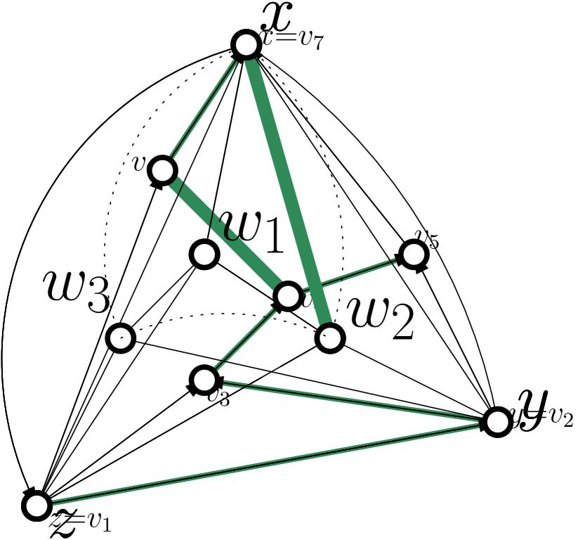
(b)

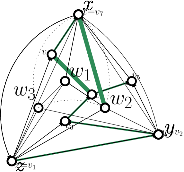
(c)

Figure 1: (a) A planar 3-connected graph with a canonical ordering [17] and the binary spanning tree obtained from it with the method in [6]. Any matching $M_{\emptyset}$ in it has size $\leq\frac{n-4}{3}$. (b) The matching-bound $|M_{x}|\geq\frac{n-2}{x}$ is tight. (c) A planar 3-connected graph with $n=6$ vertices has a matching $M_{x}$ of size 2.

The second ingredient to the proof is the result that every connected graph with minimum degree 3 has a matching of size at least $\frac{n-1}{3}$ [8]. It is not known how to find such a matching in time faster that any general-purpose maximum matching algorithm in arbitrary graphs, but the result is used here only in tree $T_{\emptyset}$. Tree $T_{\emptyset}$ is connected and has maximum degree 3, and so it contains a matching $M_{\emptyset}$ of size at least $\frac{n(T_{\emptyset})-1}{3}=\frac{n-4}{3}$. Also, in a tree a maximum matching can be found in linear time with a straightforward dynamic programming algorithm (see also [2]), so $M_{\emptyset}$ can be found in linear time.

This proves (2), and (1) is proved in the same way by using tree $T_{x}:=T\setminus\{y,z\}$ instead. ∎

The bound of Lemma 1(2) is tight, see for example Figure 1(a). The bound for Lemma 1(1), on the other hand, can be improved slightly, to $\frac{n-2}{3}$. Such a minor improvement could be deemed not be worth the effort, but is of vital importance when it it comes to merging 3-connected components of a 2-connected graph

Lemma 2

Let $G$ be a 3-connected planar graph where the outer-face contains a vertex $x$ and an edge $(y,z)$ with $y\neq x\neq z$. If $n\geq 4$, then $G$ has a matching $M_{x}$ of size at least $\frac{n-2}{3}$ where $y$ and $z$ are unmatched. It can be found in linear time.

Proof

Note that it suffices to prove the existence of such a matching; to find it in linear time use matching $M_{x}^{\prime}$ of size at least $\frac{n-3}{3}$ that exists by Lemma 1(1) and then (if needed) run one round of Edmond’s blossom algorithm to increase its size by 1. This gives the matching in linear time.

To show that matching $M_{x}$ exists, consider cases. First, if $n\not\equiv 3\bmod 3$, then by integrality $|M_{x}^{\prime}|\geq\lceil\frac{n-3}{3}\rceil\geq\frac{n-2}{3}$ and the result holds. Second, if $n\geq 8$, then it is known [8] that $G$ has a matching $M$ of size at least $\frac{n+4}{3}$. Removing from $M$ the (at most two) edges that are incident to $y$ and $z$ hence gives a matching of size at least $\frac{n-2}{3}$. By $n\geq 4$ this leaves only the case $n=6$. One could now obtain the result by enumerating all possible 3-connected graphs on $6$ vertices, but the following gives an explicit proof (see Figure 1(c)).

Let $w_{1},w_{2},w_{3}$ be the three vertices of $G$ that are not $\{x,y,z\}$. By Lemma 1(2) there is a matching $M_{\emptyset}$ of size 1 among $\{w_{1},w_{2},w_{3}\}$, after renaming therefore $(w_{1},w_{2})$ is an edge. If $(x,w_{3})$ is an edge then $(w_{1},w_{2})\cup(w_{3},x)$ is the desired matching, so assume that $(x,w_{3})\not\in E$. Since the graph is 3-connected and $n=6$, vertex $x$ has $\deg(x)\geq 3$, so $x$ is adjacent to at least one of $w_{1},w_{2}$. After renaming therefore assume that $(w_{1},x)$ is an edge. If $(w_{2},w_{3})\in E$, then $(x,w_{1})\cup(w_{2},w_{3})$ is the desired matching, so assume $(w_{2},w_{3})\not\in E$. By $\deg(w_{3})\geq 3$ therefore $w_{3}$ must be adjacent to $w_{1},y,z$. If $(x,w_{2})$ is an edge, then $(x,w_{2})\cup(w_{1},w_{3})$ is the desired matching, so assume $(x,w_{2})\not\in E$. By minimum degree 3 (and since neither $x$ nor $w_{2}$ is adjacent to $w_{3}$) therefore $x$ and $w_{2}$ must both be adjacent to all of $w_{1},y,z$. But now there is a complete bipartite graph $K_{3,3}$ with sides $\{w_{1},y,z\}$ and $\{x,w_{2},w_{3}\}$ in the planar graph $G$, a contradiction. ∎

The reader may be a bit disappointed by this proof, because it uses the Tutte-Berge formula (by appealing to the result of Nishizeki and Baybars [20]) and relies on Edmonds’ blossom algorithm [14], if only for one round. Both can be avoided by inspecting how binary spanning trees can be obtained and finding one extra edge via a counting argument. (Details are omitted, but the appendix has a similar proof for graphs with minimum degree 4.) Unfortunately the resulting linear-time algorithm, while avoiding the blossom algorithm, is also not simple since it needs to compute a so-called Tutte path.

3.2 2-connected graphs

For 2-connected graphs, it suffices to exclude two vertices on the outer-face.

Lemma 3

Let $G$ be a 2-connected planar graph with minimum degree 3 where the outer-face contains a vertex $x$ and an edge $(y,z)$ with $y\neq x\neq z$. Then $G$ has a matching $M_{x}$ of size at least $\frac{n-2}{3}$ where $y,z$ are unmatched. It can be found in linear time.

Proof

The claim holds by Lemma 2 if $G$ is 3-connected, so assume that it is not. The idea to find a $M_{x}$ is fairly standard: compute the 3-connected components, find a large matching in them, and then merge the matchings. However, two details are unusual. First, the so-called S-nodes will create difficulties because their matchings are not big enough. Therefore a pre-processing step (illustrated in Figure 2) modifies the graph by inserting artificial edges such that there are no S-nodes. This creates a complication, because the algorithm to find matching $M_{x}$ later must ensure that $M_{x}$ does not use artificial edges. Second, the matchings in the 3-connected components might well use so-called virtual edges that do not exist in $G$; such virtual edges must be removed from the matchings and compensated for by using bigger matchings in adjacent 3-connected components. (This necessitates parsing 3-connected components in a particular order, rather than simply putting the matchings together.)

SPQR-trees:

Recall first the definition of 3-connected components and the associated SPQR-tree, see for example [4, 15]. Let $G$ be a graph that that is not 3-connected, and let $(u,v)$ be a cutting pair, i.e., $G-\{u,v\}$ splits into (possibly many) connected components $C_{1},\dots,C_{k}$. The cut-components of $(u,v)$ are the subgraphs $C_{1}^{+},\dots,C_{k}^{+}$ obtained by taking for $i=1,\dots,k$ the subgraph $C_{i}$ and adding to it the vertices $u,v$ and all edges from them to $C_{i}$. Also add a virtual edge $(u,v)$ to subgraph $C_{i}^{+}$. Finally, if $k\geq 3$ or if edge $(u,v)$ exists in $G$, then define one more cut-component to consist of vertices $(u,v)$ with $k$ virtual edges $(u,v)$ (as well as the edge $(u,v)$ if it existed in $G$). Each cut-component that has at least four vertices is again 2-connected; repeat the process within them.

The 3-connected components of graph $G$ are the graphs obtained by repeating this process until all resulting graphs are multiple edges or triangles or 3-connected simple planar graphs with at least four vertices. For each 3-connected component $C$, create a node $\mu$ and set $\mathit{skel}(\mu)=C$; note that $\mathit{skel}(\mu)$ includes virtual edges. Classify each node $\mu$ as follows: $\mu$ is a P-node if $\mathit{skel}(\mu)$ has two vertices and at least three parallel edges, it is an S-node if $\mathit{skel}(\mu)$ is a triangle, and it is an R-node if $\mathit{skel}(\mu)$ is a 3-connected simple graph with at least 4 vertices. Note that any virtual edge was created as two copies, hence exists in two 3-connected components; connect two nodes $\mu,\nu$ if they have a virtual edge in common. One can argue that the result is a tree ${\cal T}$, called SPQR-tree. The SPQR-tree and the 3-connected components can be found in linear time [15].

Root the SPQR-tree ${\cal T}$ at the node $\rho$ that contains the edge $(y,z)$ and set this edge to be the parent-edge of root-node $\rho$. For all other nodes $\mu$ in ${\cal T}$, the parent-edge $(u_{\mu},v_{\mu})$ is the unique virtual edge that $\mu$ has in common with its parent in ${\cal T}$.

Eliminating S-nodes:

As explained above, any S-node $\mu$ has to be eliminated by inserting artificial edges, because the process later inserts a matching of $\mathit{skel}(\mu)$ that does not use the ends of the parent-edge, and in an S-node this would add no matching-edge at all.

Process S-nodes in top-down order in ${\cal T}$. Let $\mu$ be an S-node that has not yet been processed, and let $(u_{\mu},v_{\mu})$ be its parent edge and $a$ be the node $\neq u_{\mu},v_{\mu}$ in the triangle $\mathit{skel}(\mu)$. At least one of the edges $(u_{\mu},a)$ and $(v_{\mu},a)$ is virtual, else $\deg_{G}(a)=2$, contradicting that the minimum degree is 3. After possible renaming, edge $(v_{\mu},a)$ is virtual in $\mathit{skel}(\mu)$. Let $\nu^{\prime}$ be the child of $\mu$ that also contains virtual edge $(v_{\mu},a)$. Set $\nu=\nu^{\prime}$ if $\nu^{\prime}$ is an R-node or an S-node, and set $\nu$ to be a child of $\nu^{\prime}$ if $\nu^{\prime}$ is a P-node. (This exists since P-nodes are never leaves of ${\cal T}$.) Since no two P-nodes are adjacent, regardless of the case now $\nu$ is not a P-node and the parent-edge of $\nu$ is $(v_{\mu},a)$. Furthermore $\mathit{skel}(\nu)$ is simple and has at least three vertices. Consider one face in $\mathit{skel}(\nu)$ that is incident to its parent-edge $(v_{\mu},a)$, and let $b\neq v_{\mu},a$ be a vertex of $\mathit{skel}(\nu)$ on this face.

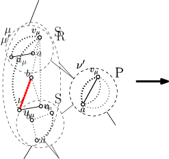
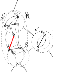
Figure 2: Eliminating an S-node $\mu$ by inserting an edge that combines $\mu$ with a child or grandchild $\nu$ to form an R-node. Parent-edges are thick dotted, other virtual edges are thin dotted, the artificial edge is red (beaded).

Add an artificial edge $(u_{\mu},b)$ to the graph. Note that one can embed $\mathit{skel}(\nu)$ inside $\mathit{skel}(\mu)$ such that $b$ is on a face incident to $(u_{\mu},v_{\mu})$, therefore the resulting graph is planar. (This requires possibly permuting the order of virtual edges on P-nodes between $\mu$ and $\nu$ and/or reversing the embedding of $\nu$.) Note that with this $\mu$ and $\nu$ becomes one R-node, whose children are the remaining children (if any) of $\mu$, all children of $\nu$, and (if $\nu^{\prime}$ was a P-node) the remaining children of $\nu^{\prime}$ (connected via a P-node if $\nu^{\prime}$ had three or more children). These changes are local to ${\cal T}$, and therefore can be executed in constant time per S-node.

Observe that if an R-node $\mu^{\prime}$ in the resulting SPQR-tree has an artificial edge $e$ in $\mathit{skel}(\mu^{\prime})$, then one end of $e$ belongs to the parent-edge of $\mu^{\prime}$ while the other is not on the parent-edge. In particular, $\mathit{skel}(\mu^{\prime})$ has a planar embedding such that the parent-edge is on the outer-face while the other end of $e$ is interior; this will be important later to avoid adding an artificial edge to the matching.

Finding the matching:

Let $G^{+}$ be the graph obtained after all S-nodes have been eliminated by the insertion of artificial edges. Let ${\cal T}^{+}$ be its SPQR-tree, with the root-node $\rho$ containing $(y,z)$. It will be helpful to expand ${\cal T}^{+}$ with a new root-node $\rho^{\prime}$ that stores two copies of $(y,z)$ (one real and one virtual) and to make $(y,z)$ virtual in $\rho$ (which becomes the child of $\rho^{\prime}$).

Now compute a matching $M_{x}$ while re-assembling $G^{+}$ from ${\cal T}^{+}$. This means the following process: Initially let the parsed subgraph $G_{p}$ be $\mathit{skel}(\rho^{\prime})$, i.e., the double edge $(y,z)$. Then, while $G_{p}$ contains virtual edges, take one virtual edge $(u,v)$ and let $\mu$ be the node of ${\cal T}^{+}$ for which this is the parent-edge. Add to $G_{p}$ the graph $\mathit{skel}(\mu)$ , and delete from $G_{p}$ the two copies of the virtual edge $(u,v)$. During this process the goal is to maintain a matching $M_{x}$ of $G_{p}$ that satisfies the following:

• $|M_{x}|\geq\frac{|G_{p}|-2}{3}$.

• Vertices $y$ and $z$ are unmatched in $M_{x}$.

• $M_{x}$ uses no artificial edge.

• $M_{x}$ uses only virtual edges for which at least one cut-component has not yet been re-inserted.

For the initial $G_{p}$ (consisting of $y,z$ and two edges between them), set $M_{x}$ to be the empty set and observe that all conditions hold. Now consider re-inserting $\mathit{skel}(\mu)$ for some node $\mu$ of ${\cal T}^{+}$, and let $(u_{\mu},v_{\mu})$ be its parent-edge. All ancestors of $\mu$ have already been re-inserted, and in particular vertices $u_{\mu}$ and $v_{\mu}$ are parsed already. Furthermore, $\mu$ is a P-node or an R-node since S-nodes have been eliminated. Expand $M_{x}$ with a matching $M_{\mu}$ inside $\mathit{skel}(\mu)$ that is found in one of three possible ways:

Case 1: $\mu$ is a P-node.

See node $\mu_{1}$ in Figure 3. In this case, do not add to matching $M_{x}$ at all. Note that no new vertices were parsed, so again $|M_{x}|\geq\frac{|G_{p}|-2}{3}$. The removal of the virtual edge $(u_{\mu},v_{\mu})$ of $\mu$ is not a problem, even if it was used by $M_{x}$, because this edge is the parent-edge of at least one child $\nu$ of $\mu$ (since $\mu$ is a P-node), and $\mathit{skel}(\nu)$ has not yet been re-inserted.

Case 2: $\mu$ is an R-node, and $(u_{\mu},v_{\mu})$ was not used by $M_{x}$ and/or exists in $G$.

See node $\mu_{2}$ in Figure 3. To find matching $M_{\mu}$, let $x_{\mu}\neq u_{\mu},v_{\mu}$ be an arbitrary vertex on the outer-face of $\mathit{skel}(\mu)$; this exists since $\mu$ is an R-node. Using Lemma 2, find a matching $M_{\mu}:=M_{x_{\mu}}(\mathit{skel}(\mu))$ that leaves $u_{\mu},v_{\mu}$ unmatched and that has size at least $\frac{|\mathit{skel}(\mu)|-2}{3}$.

Since $M_{\mu}$ leaves the ends of the parent-edge unmatched, it does not use the artificial edge that may exist inside $\mathit{skel}(\mu)$, and it does not use an edge incident to $y$ or $z$ (since these belong to the root-node, they are either not in $\mathit{skel}(\mu)$ or are an end of the parent-edge of $\mu$). All endpoints of edges in $M_{\mu}$ are in $\mathit{skel}(\mu)\setminus\{u_{\mu},v_{\mu})$, hence newly parsed, hence not matched by $M_{x}$. So $M_{x}\cup M_{\mu}$ is a matching of the required size. It does not use the virtual edge $(u_{\mu},v_{\mu})$ by case assumption, so it satisfies all required conditions.

Case 3: $\mu$ is an R-node, and $(u_{\mu},v_{\mu})\in M_{x}$ is not an edge of $G$.

See node $\mu_{3}$ in Figure 3. Since the virtual edge $(u_{\mu},v_{\mu})$ will be removed from the current graph, it must also be removed from $M_{x}$; therefore matching $M_{\mu}$ in $\mathit{skel}(\mu)$ must compensate for this removed edge and must be bigger than in the previous case. Note first that $(u_{\mu},v_{\mu})\in M_{x}$ implies that neither of its endpoints is $y$ or $z$, so $y,z$ are not vertices of $\mathit{skel}(\mu)$ and the second condition on $M_{x}$ holds. There may or may not be an artificial edge in $\mathit{skel}(\mu)$; if there is one then exactly one of its ends is in $\{u_{\mu},v_{\mu}\}$. Set $y_{\mu}\in\{u_{\mu},v_{\mu}\}$ to be this end (if there is an artificial edge) or an arbitrary vertex in $\{u_{\mu},v_{\mu}\}$ otherwise, and set $x_{\mu}$ to be the other vertex in $\{u_{\mu},v_{\mu}\}$.

Let $z_{\mu}$ be the neighbour of $y_{\mu}$ that is distinct from $x_{\mu}$ and on the outer-face of $\mathit{skel}(\mu)$; this exists since $\mu$ is a R-node. Set $M_{\mu}$ to be the matching $M_{x_{\mu}}(\mathit{skel}(\mu))$ with respect to these three vertices, i.e., $y_{\mu}$ and $z_{\mu}$ are unmatched in $M_{\mu}$. (In particular, the artificial edge has not been used.) The artificial edge (if any) is also not edge $(y_{\mu},z_{\mu})$, since one of its ends is interior to $\mathit{skel}(\mu)$. Now update $M_{x}^{\prime}:=M_{x}\setminus(u_{\mu},v_{\mu})\cup M_{\mu}\cup(y_{\mu},z_{\mu})$ and verify all claims. In particular, the size is at least $\frac{|G_{p}|p-2}{3}-1+\frac{|\mathit{skel}(\mu)|-2}{3}+1$, which is sufficiently large since $|\mathit{skel}(\mu)|-2$ new vertices were parsed.

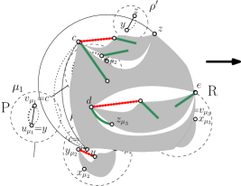
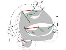
Figure 3: Re-assembling the graph while computing a matching.

Repeat the process until $G^{+}$ has been completely re-assembled. The resulting matching $M_{x}^{+}$ is a matching of size at least $\frac{n-2}{3}$ where $y,z$ are unmatched and no artificial edges are used. Since the 3-connected components can be found in linear time, and matching $M_{x}$ is obtained by computing a matching in each 3-connected component, the overall run-time is linear. ∎

3.3 Proof for connected graphs

Theorem 1.1 can now finally be proved by arguing how to handle cut-vertices; this uses more or less the “standard” approach of splitting a graph into 2-connected components and putting matchings together, but again some artificial edges need to be inserted to ensure that 2-connected components are sufficiently big.

Proof

(of Theorem 1.1) Let ${\cal B}$ be the block-tree of $G$, i.e., create a node for every 2-connected component (the maximal 2-connected subgraphs) and a node for every cut-vertex (a vertex $v$ such that $G\setminus v$ is not connected), and add an edge from a cut-vertex $v$ to a 2-connected component $C$ if and only if $v\in C$. As the name suggests, ${\cal B}$ is a tree, and it can be computed in linear time [16]. Let $C_{R}$ be a leaf of ${\cal B}$; this is necessarily a 2-connected component with at least four vertices by minimum degree 3. Root the block-tree at $C_{R}$. Let $(y,z)$ be an edge in $C_{R}$, and after possible change of embedding, assume that $(y,z)$ is on the outer-face of $G$. Declare $y$ to be the parent-node of $C_{R}$; for any 2-connected component $C\neq C_{R}$ the parent-node is the cut-vertex stored at the parent of $C$ in the block-tree.

Eliminating bridges:

A bridge is a 2-connected component that contains a single edge $(u,v)$. A pre-processing step (illustrated in Figure 4(a-b)) eliminates these in top-down order in the block-tree ${\cal B}$; Let $C$ be a 2-connected component that contains only a bridge $(u,v)$. By minimum degree 3 both $u$ and $v$ are cut-vertices, so after possible renaming $u$ is the parent-node of $C$ and $v$ is a child of $C$. Let $C^{\prime}$ be a child of $v$ and let $w$ be a neighbour of $v$; one can embed $C^{\prime}$ such that $(v,w)$ is on the outer-face of $C^{\prime}$. Insert an artificial edge $(u,w)$ and note that the result is again planar. Furthermore, this combines $C$ and $C^{\prime}$ into one 2-connected component whose parent-node is again $u$; it inherits all children of $C^{\prime}$, and also inherits $v$ as child if there are any other 2-connected components containing $v$. This is again a local change to the block-tree that can be done in overall linear time. For future reference, note that any artificial edge in a 2-connected component $C$ is adjacent to the parent-node of $C$.

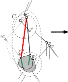
(a)

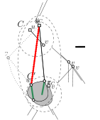
(b)

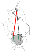
(c)

Figure 4: (a-b) Eliminating a bridge $C$ by inserting an edge that combines $C$ with a grandchild $C^{\prime}$. Parent-node are denoted by squares. (c) Finding a matching.

Finding the matching:

Now, similar as for 2-connected graphs, re-assemble the graph from the 2-connected components while creating a matching. During this process compute a matching $M_{x}$ that satisfies the following:

• $|M_{x}|\geq\frac{|G_{p}|-2}{3}$, where $G_{p}$ is the graph that has been parsed so far.

• Vertices $y$ and $z$ are unmatched in $M_{x}$.

• $M_{x}$ uses no artificial edge.

Initialize $M_{x}$ with a matching in $C_{R}$ that leaves $y$ and $z$ unmatched. Since $C_{R}$ has at least four vertices, this has size at least $\frac{|C_{R}|-2}{3}$ by Lemma 3. This uses no artificial edge since such an edge is necessarily adjacent to $y$ or $z$. So all conditions are satisfied.

Now consider some 2-connected component $C$, and let $y_{C}$ be its parent-node; $|C|\geq 3$ since there are no bridges. All ancestors of $C$ in ${\cal B}^{+}$ have already been re-inserted, and in particular $y_{C}$ has been parsed. Expand $M_{x}$ with a matching $M_{C}$ inside $C$ that is found as follows (see also Figure 4(c)): Temporarily add a vertex $z_{C}$ in the outer-face of $C$, and connect it to $y_{C}$ and to two other vertices on the outer-face of $C$ in such a way that edge $(y_{C},z_{C})$ is on the outer-face of the resulting graph $C^{+}$. Let $x_{C}\neq y_{C},z_{C}$ be an arbitrary vertex on the outer-face of $C^{+}$. Since $|C^{+}|\geq 4$ and $C^{+}$ is 2-connected, use Lemma 3 to find a matching $M_{C}:=M_{x_{C}}(C^{+})$ of $C^{+}$ where $y_{C}$ and $z_{C}$ are unmatched such that $|M_{C}|\geq\frac{|C^{+}|-2}{3}=\frac{|C|-1}{3}$. All vertices matched by $M_{C}$ are in $C\setminus\{y_{C},z_{C}\}$, hence newly parsed, hence not matched by $M_{x}$. Since $|C|-1$ vertices were newly parsed, therefore $M_{x}^{\prime}:=M_{x}\cup M_{C}$ is sufficiently big. Finally, since $y_{C}$ is unmatched in $M_{x}$, the artificial edge (if any) in $C$ is not used by $M_{C}$. So all conditions hold.

Repeat the process until $G^{+}$ has been completely re-assembled. The resulting matching $M_{x}$ is a matching of size at least $\frac{n-1}{3}$ in $G$ where $y,z$ are unmatched and no artificial edges are used. Finally add $(y,z)$ to this matching; this gives a matching in $G$ of size $\frac{n+1}{3}$ as desired. Since the 2-connected components can be found in linear time, and matching $M_{x}$ is obtained by computing a matching in each 2-connected component, the overall run-time is linear. ∎

4 Higher minimum degree?

Nishizeki and Baybars [20] proved larger matching-bounds for higher minimum degree, in particular 3-connected planar graphs have matchings of size at least $\frac{3}{7}n$ if the minimum degree is 4. Their proof uses the Tutte-Berge-formula, so naturally one wonders whether these matchings can be found in linear time. This remains an open problem. Lemma 4 below states that a slightly smaller matching can be found in linear time. This result is not new: Applying Baker’s approximation scheme [2] with $\varepsilon=\frac{1}{15}$ will gives a matching of size at least $\left(1-\frac{1}{15}\right)\frac{3}{7}n=\frac{6}{15}n$ in time $O(8^{15}n)$. Since $8^{15}$ is a constant (albeit large), this is linear time. The interesting part of Lemma 4 is hence not the result, but its proof; the hope is that with minor modifications it could be used to find a matching of size $\frac{3}{7}n$ in 3-connected planar graphs with minimum degree 4.

Lemma 4

Let $G$ be a triangulated planar graph with $n>3$ where the outer-face consists of $\{x,y,z\}$ and all interior vertices have degree at least 4. Then $G$ has

• a matching $M_{x}$ of size at least $\frac{6n-15}{15}$ where $y,z$ are unmatched.

• a matching $M_{\emptyset}$ of size at least $\frac{6n-21}{15}$ where $x,y,z$ are unmatched.

They can be found in linear time.

Proof

(Sketch, details can be found in the appendix.) Let $P$ be a Tutte-path, which is a path such that any component $C$ of $G\setminus P$ has only three neighbours on $P$, hence resides inside a separating triangle $T_{C}$ (a triangle of $G$ that is not a face). Furthermore, each component $C$ has a representative $\sigma(C)$, which is a vertex in $P$ such that no two components use the same representative. For each component $C$, let $C^{+}$ be the graph induced by $T_{C}\cup C$. Recursively compute $M_{\emptyset}(C^{+})$ and $M_{\sigma(C)}(C^{+})$.

Now take every other edge of $P$, say $(v_{i-1},v_{i})$ is such an edge. If neither $v_{i-1}$ nor $v_{i}$ is used as representative, then add $(v_{i-1},v_{i})$ to $M$; this adds one matching-edge for two vertices. If $v_{i-1}$ and/or $v_{i}$ is used as representatives, say for components $C_{i-1}$ and/or $C_{i}$, then add the matchings of these components. Evaluating the constants exactly, one can verify that this adds $\frac{6(|C_{i}|+|C_{i-1}|+2)}{15}$ matching-edges for the $|C_{i}|+|C_{i-1}|+2$ vertices in $C_{i}\cup C_{i-1}\cup\{v_{i-1},v_{i}\}$. Repeating this for every other edge of $P$ gives a matching of size $\frac{6|V|}{15}-c$ (where the error term $-c$ occurs if $P$ has an even number of edges). This error-term is a bit too big for the desired bound, but one can argue (by re-arranging which matchings are used) that it can be decreased to be at most $-\frac{3}{15}$.

To ensure that $y,z,$ and (maybe) $x$ are unmatched, path $P$ must be chosen so that it begins at $x$ and ends with $(y,z)$. Then use $P\setminus\{y,z\}$ or $P\setminus\{x,y,z\}$ as path in the above arguments and the desired bound follows. ∎

5 Outlook

This paper considered the problem of finding large matchings in a planar graph with minimum degree 3. It was known that any such graph has a matching of size at least $\frac{n+2}{3}$, but all previous proofs were non-constructive and relied on generic maximum-matching-finding algorithms to construct such a matching. This paper re-proves the result (for varying levels of connectivity), and the proofs naturally lead to linear-time algorithms to find the matching.

As for open problems, a number of other matching bounds have been proved using the Tutte-Berge formula, sometimes for graph classes that are not even planar:

• As mentioned earlier, every 3-connected planar graph has a matching of size at least $\frac{3}{7}n$ if $n\geq 30$ and the minimum degree is 4, and of size at least $\frac{9}{19}n$ if $n\geq 78$ and the minimum degree is 5 [20].

• Any 3-connected planar graphs have a matching of size $(2n-\ell_{4})/4$, where $\ell_{4}$ is the number of leaves in the tree ${\cal T}_{4}$ of 4-connected components [8].

• Every Delauney triangulation has a matching of size $\lceil(n-1)/2\rceil$ [13].

• Every $\Theta_{6}$-graph has a matching of size at least $\frac{3}{7}n$ [7].

• Every maximal simple 1-planar graph has a matching of size at least $\frac{2}{5}n$, and there are also matching bounds for 1-planar graphs of minimum degree 3,4, or 5 [24].

For all these results, the following question remains open: Can such matchings be bound in linear time?

Appendix 0.A Triangulated graphs with minimum degree 4

This appendix gives a proof of Lemma 4, i.e., a triangulated graph with minimum degree 4 has a matching of size at least $\frac{6}{15}n$ that can be found in linear time. More precisely, for $X=\{y,z\}$ or $X=\{x,y,z\}$ the goal is to find a matching $M_{X}$ of size $\frac{6(n-|X|)-3}{15}$ where vertices in $X$ are unmatched.

Base case:

The proof proceeds by induction on the number of separating triangles. In the base case, $G$ has no separating triangles, and therefore is 4-connected. In turns out that the induction step given below can also cover the base case, so we will not write the argument here.

Tutte path background:

The matching is found using a so-called Tutte-path $P$, which is a generalization of a Hamiltonian path, exists in 2-connected planar graphs [22] and can be found in linear time [9]. The following statement holds for all 3-connected planar graphs (even if not triangulated), and needs the notion of a separating triplet, i.e., a set $T$ of three vertices such that $G\setminus T$ is not connected.

Theorem 0.A.1 ([9])

Let $G$ be a 3-connected planar graph where the outer-face contains a vertex $x$ and an edge $(y,z)$ with $y\neq x\neq z$. Then $G$ has a path $P$ that begins with $x$ and ends with edge $(y,z)$ such that the following holds for the connected components ${\cal C}$ of $G\setminus P$:

• For any $C\in{\cal C}$, there exists a separating triplet $T_{C}=\{x_{C},y_{C},z_{C}\}$ of $G$ such that $C$ is a component of $G\setminus T_{C}$ and the vertices of $T_{C}$ are on $P$.

• There exists an injective assignment $\sigma(C):{\cal C}\rightarrow P$ of representatives such that $\sigma(C)\in T_{C}\setminus\{x,y,z\}$.

Furthermore, $P$ and the representatives can be found in time $O(\sum_{f\in{\cal F}(P)}\deg(f))$, where ${\cal F}(P)$ is the set of interior faces of $G$ that contain a vertex of $P$.

Assume for the rest of the proof that one such path $P$ has been fixed. Note that vertices in $X$ are the first or last vertices of $P$, so $P\setminus X$ is also a path and can be enumerated as $\langle v_{0},v_{1},v_{2},\dots,v_{k}\rangle$. See also Figure 5. Observe that $n\geq 4$ implies $|P|\geq 4$, otherwise any interior vertex is in some component $C\in{\cal C}$, but $\sigma(C)\in P\setminus\{x,y,z\}$, which is then impossible. So $P\setminus X$ is non-empty and $k\geq 0$. On the other hand, ${\cal C}$ may well be empty (e.g. in the base case when there are no separating triangles).

If ${\cal C}$ is non-empty, then for each $C\in{\cal C}$ let $T_{C}$ be the separating triangle that encloses $C$, and let $C^{+}$ be the subgraph induced by $C\cup T_{C}$. Since $C^{+}$ is triangulated, has fewer separating triangle, and all its interior vertices have degree 4 or more, one can obtain matchings $M_{\emptyset}(C^{+})$ and $M_{v}(C^{+})$ for $v\in T_{C}$ recursively. Classify $C$ as one of two types: $C$ is outward if $6|C|\%15\in\{1,2,3\}$ and inward otherwise, where $\%$ denotes the modulo-operator. Usually an inward component $C$ will use $M_{\emptyset}(C^{+})$ while an outward component will use $M_{\sigma}(C)(C^{+})$, but some exceptions will be made to this below.

Pre-processing:

Before computing the matching, the assignment $\sigma(\cdot)$ of representatives should get changed so that, whenever possible, an even-indexed vertex is used. More precisely, assume that some $C\in{\cal C}$ satisfies the following: $\sigma(C)$ is $v_{2s+1}$, some other vertex of $T_{C}$ is $v_{2t}$, and there is no $C^{\prime}\in{\cal C}$ with $\sigma(C^{\prime})=v_{2t}$. Then change the system of representatives and set $\sigma(C):=v_{2t}$. For example, in Figure 5(a), one can reassign $C_{6}$ to use $v_{6}$, rather than $v_{7}$, as representative.

(a)

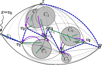
(b)

Figure 5: Finding $M_{x}$. Path $P$ is blue dashed, the representatives are purple arrows. (a) $k$ is odd, so use $M_{0,1},M_{2,3},M_{4,5}$ and $M_{6,7}$. (b) $k$ is even and $C_{2}$ is non-empty, so use $M_{0,1}$, $M_{2}$, $M_{3,4}$ and $M_{5,6}$.

Matchings $M_{i}$ and $M_{i-1,i}$:

For $i=0,\dots,k$, let $C_{i}$ be the component in ${\cal C}$ for which $\sigma(C_{i})=v_{i}$. If there is no such component then set $C_{i}:=\emptyset$ (an empty component). Also set $V_{i}:=V(C_{i})\cup\{v_{i}\}$. Observe that $\bigcup_{i=0}^{k}V_{i}=V\setminus X$ since no component uses a vertex of $X\subseteq\{x,y,z\}$ as a representative. Since the goal is to find a matching $M$ of size $\frac{6(n-|X|)-3}{15}$, it suffices to find for $i=0,\dots,k$ a matching in $V_{i}$ of size $\frac{6|V_{i}|}{15}$. This is not always possible (e.g. if $C_{i}$ is empty), but the idea is to achieve this bound on average.

For $i=0,\dots,k$, define matching $M_{i}$ as follows. If $C_{i}$ is empty then set $M_{i}:=\emptyset$ and observe that $|M_{i}|=0=\frac{6|V_{i}|-6}{15}$. If $C_{i}$ is inward, then set $M_{i}:=M_{\emptyset}(C_{i}^{+})$, and observe that $|M_{i}|\geq\lceil\frac{6|C^{+}_{i}|-21}{15}\rceil=\lceil\frac{6|C_{i}|-3}{15}\rceil$ by integrality. But $6|C_{i}|\%15\neq 1,2,3$ by definition of “inward”, so actually $|M_{i}|\geq\frac{6|C_{i}|}{15}=\frac{6|V_{i}|-6}{15}$. Finally if $C_{i}$ is outward, then set $M_{i}:=M_{v_{i}}(C_{i}^{+})$. By integrality $|M_{i}|\geq\lceil\frac{6|C_{i}^{+}|-15}{15}\rceil=\lceil\frac{6|C_{i}|+3}{15}\rceil$. Since $6|C_{i}|\%15\in\{1,2,3\}$, hence $\lceil\frac{6|C_{i}|+3}{15}\rceil\geq\frac{6|C_{i}|+12}{15}=\frac{6|V_{i}|+6}{15}$. Summarizing, for $i\in\{0,\dots,k\}$,

$$|M_{i}|\geq\left\{\begin{array}[]{ll}\frac{6|V_{i}|+6}{15}&\mbox{if $C_{i}$ is outward}\\[5.16663pt] \frac{6|V_{i}|-6}{15}&\mbox{if $C_{i}$ is inward or empty}\end{array}\right.$$ (1)

Furthermore, $v_{i}$ is unmatched in $M_{i}$ unless $C_{i}$ is outward.

For $i=1,\dots,k$, define a matching $M_{i-1,i}$ within $V_{i-1}\cup V_{i}$ as follows: If both $C_{i-1}$ and $C_{i}$ are empty or inward, then set $M_{i-1,i}=(v_{i-1},v_{i})\cup M_{i-1}\cup M_{i}$; this is a matching since $v_{i-1}$ and $v_{i}$ are unmatched in $M_{i-1}$ and $M_{i}$. In this case, $|M_{i-1,i}|\geq 1+\frac{6|V_{i-1}|-6}{15}+\frac{6|V_{i}|-6}{15}=\frac{6(|V_{i-1}|+|V_{i}|)+3}{15}$. Otherwise, set $M_{i-1,i}=M_{i-1}\cup M_{i}$ and observe that this has size at least $\frac{6|V_{i-1}|-6}{15}+\frac{6|V_{i}|+6}{15}$ since at least one of $C_{i-1}$ and $C_{i}$ is outward. So for $i=1,\dots,k$

$$|M_{i-1,i}|\geq\left\{\begin{array}[]{ll}\frac{6(|V_{i-1}|+|V_{i}|)+3}{15}&\mbox{if neither $C_{i-1}$ nor $C_{i}$ is outward}\\[5.16663pt] \frac{6(|V_{i-1}|+|V_{i}|)}{15}&\mbox{otherwise}\end{array}\right.$$ (2)

Combining matchings:

The following cases show how to put these matchings together to obtain the desired bound:

Case 1:

$k$ is odd. Then use $M=M_{0,1}\cup M_{2,3}\cup\dots\cup M_{k-1,k}.$ By Inequality (2) then $|M|\geq\sum_{i=0}^{k}\frac{6|V_{i}|}{15}=\frac{6(n-|X|)}{15}$ as desired.

Case 2:

$k$ is even and $C_{2s}$ is non-empty for some $s=0,\dots,k/2$. Then use

$$M=M_{0,1}\cup\dots\cup M_{2s-2,2s-1}\cup M_{v_{2s}}(C^{+}_{2s})\cup M_{2s+1,2s+2}\cup\dots\cup M_{k-1,k}.$$

Note that regardless of whether $C_{2s}$ is inward or outward, we have $|M_{v_{s}}(C^{+}_{2s})|\geq\frac{6|C_{2s}^{+}|-15}{15}=\frac{6|V_{2s}|-3}{15}$. Combining this with Inequality (2) applied to all other parts of $M$ shows that $|M|\geq\sum_{i=0}^{k}\frac{6|V_{i}|}{15}-\frac{3}{15}=\frac{6(n-|X|)-3}{15}$ as desired.

Case 3:

$k$ is even, and $C_{2s+1}$ and $C_{2s+2}$ are both empty or inward for some $0\leq s\leq k/2-1$. Set

$$M=M_{0,1}\cup\dots\cup M_{2s-2,2s-1}\cup M_{2s}\cup M_{2s+1,2s+2}\cup\dots\cup M_{k-1,k}.$$

(This is almost the same matching as in the previous case, but the analysis is different.) The stronger bound in Inequality (2) applies to $M_{2s+1,2s+2}$, so

$$|M_{2s}|+|M_{2s-2,2s-1}|\geq\frac{6|V_{2s}|-6}{15}+\frac{6(|V_{2s+1}|+|V_{2s+2}|)+3}{15}.$$

Combining this with Inequality (2) applied to all other parts of $M$ shows that $|M|\geq\sum_{i=0}^{k}\frac{6|V_{i}|}{15}-\frac{3}{15}=\frac{6(n-|X|)-3}{15}$ as desired.

Case 4:

$k$ is even, and for some $0\leq s<t\leq k/2$ edge $(v_{2s},v_{2t})$ exists and $C_{2s}$ and $C_{2t}$ are empty. Then use

$$M = M_{0,1}\cup\dots\cup M_{2s-2,2s-1}\quad\cup\quad(v_{2s},v_{2t})\cup M_{2s+1}$$

$$\cup M_{2s+2,2s+3}\cup\dots\cup M_{2t-2,2t-1}\quad\cup\quad M_{2t+1,2t+2}\cup\dots\cup M_{k-1,k}.$$

See also Figure 6(b). Note that $(v_{2s},v_{2t})\cup M_{2s+1}$ resides within $V_{2s}\cup V_{2s+1}\cup V_{2t}$, and $|V_{2s}|=|V_{2t}|=1$ since $C_{2s}$ and $C_{2t}$ are empty, so

$$1{+}|M_{2s+1}|\geq\frac{6(|V_{2s}|{+}|V_{2t}|){+}3}{15}{+}\frac{6|V_{2s+1}|-6}{15}=\frac{6(|V_{2s}|{+}|V_{2s+1}|{+}|V_{2t}|)-3}{15}.$$

Combining this with Inequality (2) applied to all other parts of $M$ shows that $M$ has size at least $\sum_{i=0}^{k}\frac{6|V_{i}|}{15}-\frac{3}{15}=\frac{6(n-|X|)-3}{15}$ as desired.

(a)

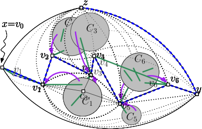
(b)

Figure 6: More methods of obtaining $M$. (a) $k$ is even and $C_{0},C_{1}$ are empty, so use $M_{0,1}\cup M_{2}\cup M_{3,4}\cup M_{5,6}$. (b) $k$ is even, edge $(v_{4},v_{6})$ exists and $C_{4},C_{6}$ are empty, so use $M_{0,1}\cup M_{2,3}\cup(v_{4},v_{6})\cup M_{5}$.

Correctness:

It remains to show that one of the above cases must apply. Assume for contradiction that none of them applies, so in particular $k$ is even (by Case 1), $C_{0},C_{2},\dots,C_{k}$ are empty (by Case 2) and $C_{1},C_{3},\dots,C_{k-1}$ are outward (by Case 3 and since $C_{0},C_{2},\dots,C_{k}$ are empty). Construct an auxiliary graph $H$ as follows (this step is only needed to argue correctness, not for the algorithm). Vertex set $A$ (shown with black squares in Figure 6(b)) consists of $X$ and $v_{1},v_{3},\dots,v_{k-1}$, a total of $\frac{k}{2}+|X|$ vertices. Vertex set $B$ (shown with circles) consists of $v_{0},v_{2},\dots,v_{k}$ and vertices $c_{1},c_{3},\dots,c_{k-1}$, where $c_{i}$ represents the (non-empty, outward) component $C_{i}\in{\cal C}$. So $|B|=k+1$. Note that $B$ includes $x=v_{0}$ if (as in Figure 6(b)) the goal is to find matching $M_{x}$.

Add the following edges to $H$. First, add any edge from $A$ to $B$ that also existed in $G$. Also connect $c_{i}$ (for $i=1,3,\dots,k-1$) to each vertex of $T_{C_{i}}$; due to the pre-processing vertices in $T_{C_{i}}$ are in $X$ or have an odd index, so $c_{i}$ has exactly three neighbours and they are in $A$.

By construction $H$ is bipartite and a minor of planar graph $G$. Since also $|H|\geq 3$, it has at most $2|H|-4=2(\frac{3}{2}k+|X|+1)-4=3k+2|X|-2$ edges. Observe that $\deg_{H}(v_{2s})\geq 4$ for all even-indexed vertices $v_{2s}$, because $v_{2s}$ has at least four neighbours in $G$, none of these can be in a component $C_{2t}$ ($C_{2t}$ is empty), none of these can be in a component $C_{2t+1}$ (else $v_{2t}\in T_{C_{2t+1}}$, but by the pre-processing $T_{C_{2t+1}}\subseteq A$) and none of them can be an even-index vertex $v_{2t}$ (else Case 4 applies). So all neighbours of $v_{2s}$ in $G$ are in $X\cup\{v_{1},v_{3},\dots,v_{k-1}\}=A$ and also neighbours in $H$. It follows that $H$ has at least $\sum_{v\in B}\deg(v)\geq 4(\frac{k}{2}+1)+3\frac{k}{2}=\frac{7}{2}k+4$ edges. Thus $\frac{7}{2}k+4\leq 3k+2|X|-2$, which implies $|X|=3$ and $k=0$. But then $|A|=3$, making $\deg_{H}(v_{0})\geq 4$ impossible. Contradiction, so one of the cases must apply.

Run-time:

Some algorithmic details remain to be filled in. Before starting any recursions, compute the tree ${\cal T}_{4}$ of 4-connected components; this can be done in linear time [18]. Root ${\cal T}_{4}$ at the component containing the outer-face, and let every node store that size of the subgraph of its descendants. With this, one can later determine in constant time whether $6|C|\%15\in\{1,2,3\}$ for any $C\in{\cal C}$, because $C$ is one component of $G\setminus T_{C}$ for a separating triangle $T_{C}$ and hence corresponds to a node of ${\cal T}_{4}$.

Finding $P$ and the representatives $\sigma$ takes time $O(\sum_{f\in{\cal F}(P)}\deg(f))$, where ${\cal F}(P)$ are the interior faces of $G$ that are incident to vertices of $P$ [9]. Next, determine triangle $T_{C}$ for each $C\in{\cal C}$ (this “falls out of” the algorithm to find $P$, but can also be re-computed by scanning the clockwise order of edges around each vertex in $P$). Then do the pre-processing to find the final assignment of representatives; note that at this point the indices of vertices in $P$ are fixed and so this can be done in $O(1)$ time per component. Finally find the graph $G[P]$ induced by $P$ and check whether it has any edges between two even-indexed vertices. Since one can also look up the type of each $C\in{\cal C}$ in constant time, one can hence determine which case applies in $O(|P|)$ time. All these operations together take time $O(|P|+\sum_{v\in P}\deg(v))$, which is $O(\sum_{f\in{\cal F}(P)}\deg(f))$ and can hence be viewed as overhead to computing $P$.

Now recursively compute for each $C\in{\cal C}$ the required matching; this takes time $O(|{\cal F}(C)|)$ time, where ${\cal F}(C)$ is the set of interior faces in $C^{+}$. Note that ${\cal F}(C)$ and ${\cal F}(P)$ overlap in faces that are incident to $T_{C}$, but similarly as in [9] it is possible to re-use the information from the computation for $P$ in the computation of the path $P_{C}$ in $C^{+}$ (which is the first step in the computation of the matching in $C^{+}$). So overall this is linear time. This finishes the proof of Lemma 4.

References

- [1] N. Anari and V. Vazirani. Planar graph perfect matching is in NC. In Symposium on Foundations of Computer Science (FOCS 2018), pages 650–661. IEEE Computer Society, 2018.
- [2] B. Baker. Approximation algorithms for NP-complete problems on planar graphs. J. ACM, 41(1):153–180, 1994.
- [3] D. W. Barnette. Trees in polyhedral graphs. Canad. J. Math., 18:731–736, 1966.
- [4] G. Di Battista and R. Tamassia. On-line planarity testing. SIAM J. Computing, 25(5), 1996.
- [5] C. Berge. Sur le couplage maximum d’un graphe. Comptes Rendus de l’Académie des Sciences, Paris, 247:258–259, 1958.
- [6] T. Biedl. Trees and co-trees with bounded degrees in planar 3-connected graphs. In Scandinavian Symposium and Workshops on Algorithms Theory (SWAT’14), volume 8503 of LNCS, pages 62–73. Springer, 2014.
- [7] T. Biedl, A. Biniaz, V. Irvine, K. Jain, P. Kindermann, and A. Lubiw. Matching and blocking sets in -graphs. 2019. CoRR 1901.01476. To appear at EuroCG’19.
- [8] T. Biedl, E. Demaine, C. Duncan, R. Fleischer, and S. Kobourov. Tight bounds on maximal and maximum matching. Discrete Mathematics, 285(1-3):7–15, 2004.
- [9] T. Biedl and P. Kindermann. Finding Tutte paths in linear time, 2018. CoRR report 1812.04543. In submission.
- [10] T. Biedl, P. Bose, E. Demaine, and A. Lubiw. Efficient algorithms for Petersen’s theorem. J. Algorithms, 38(1):110–134, 2001.
- [11] G. Borradaile, P. Klein, S. Mozes, Y. Nussbaum, and C. Wulff-Nilsen. Multiple-source multiple-sink maximum flow in directed planar graphs in near-linear time. SIAM Journal on Computing, 46(4):1280–1303, 2017.
- [12] N. Chiba and T. Nishizeki. The Hamiltonian cycle problem is linear-time solvable for -connected planar graphs. J. Algorithms, 10(2):187–211, 1989.
- [13] M. Dillencourt. Toughness and Delaunay triangulations. Discrete & Computational Geometry, 5:575–601, 1990.
- [14] J. Edmonds. Paths, trees, and flowers. Canad. J. Math., 17:449–467, 1965.
- [15] C. Gutwenger and P. Mutzel. A linear time implementation of SPQR-trees. In Graph Drawing (GD 2000), volume 1984 of Lecture Notes in Computer Science, pages 77–90. Springer, 2000.
- [16] J. E. Hopcroft and R. E. Tarjan. Efficient algorithms for graph manipulation. Communications of the ACM, 16(6), June 1973.
- [17] G. Kant. Drawing planar graphs using the canonical ordering. Algorithmica, 16:4–32, 1996.
- [18] G. Kant. A more compact visibility representation. Internat. J. Comput. Geom. Appl., 7(3):197–210, 1997.
- [19] S. Micali and V. V. Vazirani. An algorithm for finding maximum matching in general graphs. In Foundations of Computer Science (FOCS’80), pages 17–27. IEEE Computer Society, 1980.
- [20] T. Nishizeki and I. Baybars. Lower bounds on the cardinality of the maximum matchings of planar graphs. Discrete Mathematics, 28(3):255–267, 1979.
- [21] W.-B. Strothmann. Bounded-degree spanning trees. PhD thesis, FB Mathematik/Informatik und Heinz-Nixdorf Institute, Universität-Gesamthochschule Paderborn, 1997.
- [22] W. T. Tutte. Bridges and Hamiltonian circuits in planar graphs. Aequationes Math., 15(1):1–33, 1977.
- [23] V. Vazirani. An improved definition of blossoms and a simpler proof of the MV matching algorithm. CoRR, abs/1210.4594, 2012.
- [24] J. Wittnebel. Bounds on maximum matchings in 1-planar graphs. Master’s thesis, University of Waterloo, January 2019. http://hdl.handle.net/10012/14445.