Critical Density of the Abelian Manna Model via a Multi-type Branching Process

Abstract

A multi-type branching process is introduced to mimic the evolution of the avalanche activity and determine the critical density of the Abelian Manna model. This branching process incorporates partially the spatio-temporal correlations of the activity, which are essential for the dynamics, in particular in low dimensions. An analytical expression for the critical density in arbitrary dimensions is derived, which significantly improves the results over mean-field theories, as confirmed by comparison to the literature on numerical estimates from simulations. The method can easily be extended to lattices and dynamics other than those studied in the present work.

I Introduction

The Manna Model Manna (1991) is the prototypical stochastic sandpile model proposed for self-organized criticality (SOC) Bak et al. (1988). It was reformulated by Dhar to make it Abelian Dhar (1999a). The resulting Abelian Manna model (AMM) and its variants have been studied extensively numerically and analytically Ben-Hur and Biham (1996); Dhar (1999b); Dickman (2002); Basu and Mohanty (2014); Wiese (2016); Willis and Pruessner (2018a). Numerical simulations have established that a range of other models belong to the same universality class (Pruessner, 2012, p. 178), in particular the Oslo Model Christensen et al. (1996); Paczuski and Boettcher (1996) and the conserved lattice gas Rossi et al. (2000a); Jensen (1990). The stationary density of the AMM has been estimated with very high precision on hypercubic lattices of dimensions $d=1$ to $d=5$ Lübeck (2000); Dickman et al. (2001); Huynh et al. (2011); Huynh and Pruessner (2012); Willis and Pruessner (2018a). Yet, theoretical understanding of the Manna Model is far from complete. In a mean-field theory which ignores all spatial-temporal correlations, the avalanches can be naturally perceived as a binary branching process (BP) Alstrøm (1988); García-Pelayo (1994) with branching ratio $\sigma$ twice the particle density $\zeta$ as a mean field. At stationarity, the macroscopic dynamics of driving and dissipation of particles self-organises the branching ratio to unity, which is the critical value, $\sigma_{c}=1$, i.e. the branching ratio above which a finite fraction of realisations branches indefinitely. The mean-field value of the critical density is therefore $\zeta_{c,\text{\scriptsize(MF)}}=\sigma_{c}/2=1/2$ regardless of the dimension of the system Zapperi et al. (1995). However, numerical findings have placed the critical value $\zeta_{c}$ of the density clearly above $1/2$ in any dimension studied Pruessner (2012); Willis and Pruessner (2018a), suggesting that the spatial correlations ignored by the mean-field theory are significant. Here, we provide a theoretical characterisation of $\zeta_{c}$ in a general setting through a mapping to a multi-type branching process (MTBP), with a simple closed-form approximation systematically improving on the mean-field prediction. Our method incorporates only short-ranged correlations during the avalanche and highlights the role that particles conservation plays in regulating activity. While still ignoring correlations in the initial state Basu et al. (2012); Hexner and Levine (2015); Willis and Pruessner (2018a), we show that taking into account even only some of the correlations arising in the activity modifies significantly the estimate of the critical density. One may hope that our findings can be reproduced to leading order in a suitable field theory.

In the following, we first introduce the Abelian Manna Model and its (approximate) mapping to the multi-type branching process mimicking (some of) its dynamics. We then demonstrate how the critical density of the AMM can be extracted from the branching process and conclude with a brief discussion of the results.

II The Abelian Manna Model

To facilitate the following discussion, we reproduce the definition of the AMM: The AMM is normally studied on a $d$-dimensional hypercubic lattice, but extensions to arbitrary graphs are straight forward. Each site carries a non-negative number of particles, which we refer to as the occupation number. A site that carries no particle is said to be empty, otherwise it is occupied by at least one particle. A site carrying less than two particles is stable, otherwise it is active. If all sites in a lattice are stable, the system is said to be quiescent, as it does not evolve by its internal dynamics. If the lattice has $N$ sites, the number of such states is $2^{N}$. Particles are added to the lattice by an external drive. If such an externally added particle arrives at a site that is occupied by a particle already, an avalanche ensues as follows: Every site that carries more than one particle topples by moving two of them to randomly and independently chosen nearest neighbours, thereby charging them with particles. This might trigger a toppling in turn. The totality of all topplings in response to a single particle added by the external drive is called an avalanche.

We will refer to the evolution from toppling to toppling as the microscopic timescale, as opposed to the macroscopic timescale of the evolution of quiescent states. The evolution from one quiescent state to another quiescent state by adding a particle at a site and letting an avalanche complete is a Markov process. Because of the finiteness of the state space of quiescent configurations and assuming accessibility of all states (but see (Willis and Pruessner, 2018b)), the probability to find the AMM in a particular quiescent state approaches a unique, stationary, strictly positive value. The analysis below is concerned solely with the the stationary state of the AMM.

For the discussion below we require the notion of occupation number pre-toppling and occupation number post-toppling. The former refers to the number of particles at a site prior to its possible toppling, the latter refers to the number of particles at a site immediately after possibly shedding (a multiple of) two particles and yet prior to it receiving particles from any other site. Committing a slight abuse of terminology, we will refer to pre- and post-toppling occupation numbers even when the site is stable.

Of particular importance to the following consideration is the occupation density $\zeta$, that the expected total number of particles divided by the number of sites.

II.1 The multi-type branching process

One paradigm of the AMM and SOC in general is the (binary) branching process Harris (1963). The population of that process at any given time is thought to represent those sites that become active as a result of receiving a particle. As they topple, the particles arriving at nearest neighbouring stable sites might activate those, depending on whether they were previously occupied by a particle or not. Any empty site that is charged with only one particle becomes occupied but remains stable. Any stable site charged with two particles is guaranteed to become active. As active sites are sparse, they are rarely charged. However, the Abelian property of the AMM means that the arrival of one additional particle at a site leads to a further toppling only if the parity of its occupation number is odd. If two particles arrive at a site, its parity will not change, but the site is bound to topple (once more).

If a neighbouring site becomes active in response to a charge, this corresponds in the branching process to an offspring in the next generation. If two such offspring are generated, this corresponds to a branching that increases the population size. If a neighbouring site turns from empty to occupied, no offspring is produced.

The spatio-temporal evolution of an avalanche may thus be thought of as a branching process embedded in space and with strong correlations of branching and extinction events as the lattice occupation dictates whether and where these events take place. Ignoring the lattice and the history of previous and ongoing avalanches, one is left with a plain binary branching processes, as it is commonly used to cast the AMM and SOC models generally in a mean field theory Zapperi et al. (1995); Lübeck (2004); Juanico et al. (2007); Bonachela and Muñoz (2009). Field theoretic treatments of any such processes always involve branching as a basic underlying process Vespignani et al. (1998); Ramasco et al. (2004).

In general branching processes, the branching ratio is exactly unity at the critical point of the process, above which the probability of sustaining a finite population size indefinitely is strictly positive. We therefore identify the critical point of the branching process with that of the lattice model.

dimension	1	2	3	5
$\zeta_{c}$ (numerically)	0.94882(1) Willis and Pruessner (2018a)	0.7170(4)Huynh et al. (2011)	0.622325(1) Huynh and Pruessner (2012)	0.559780(5) Willis and Pruessner (2018a)
$\zeta_{c}$ (present work)	0.750	0.625	0.583	0.550

Table 1: The theoretical estimate of the critical density $\zeta_{c}$ in the $d$-dimensional AMM derived here compared to the numerical values reported in the literature for the stationary density of the Abelian Manna Model.

             

             

Figure 1: The six different active motives of the one-dimensional Abelian Manna Model. The central site carries either three ($\alpha_{i}$ for $i=0,1,2$) or two particles ($\beta_{i}$ for $i=0,1,2$) and is to topple in the next microscopic time step. The occupation number of sites neighbouring the central site are representative only in as far as their parity is concerned, with $i$ indicating the number of sites that carry an odd number. Their occupation number is post-toppling (after they may have toppled themselves, but prior to the central site toppling), whereas the central site is shown pre-topping (before it topples). The configurations differ in whether neighbouring sites may or may not topple themselves due to being charged by the toppling site. Although we may picture the configurations being situated on a one-dimensional lattice, their spatial orientation is irrelevant and so we do not distinguish left and right neighbours.

The multi-type branching process considered in the following is based on a mapping of the types (or species) of the branching process to the active motives of the AMM, as shown in Figure 1 for the one-dimensional case. These motives indicate the occupation number of the central site pre-toppling (i.e. prior to the central site toppling) and the occupation of the neighbouring sites post-toppling (i.e. after they may have toppled themselves, which leaves their parity unchanged, but prior to the central site toppling). Defining the motives this way, we can disregard toppling sites charging active neighbouring sites. We effectively keep track only of the change of parity of the neighbouring sites, which is due to charges they receive but does not change when they topple themselves. Within a time step in the multi-type branching process all currently active motives undergo toppling, which corresponds to parallel updating on the microscopic time scale of the AMM.

The species labels in Figure 1 of the form $\sigma_{i}$ characterise the configuration as follows: $\sigma=\alpha$ indicates that the active site carries three particles, $\sigma=\beta$ indicates that it carries two. The index $i$ indicates the number of neighbouring sites carrying a single particle post-toppling. In general, $i\in\{0,\ldots,q\}$ where $q$ is the coordination number. Henceforth, we restrict ourselves to regular lattices with constant coordination number $q$. These may be thought of as $d$-dimensional hypercubic lattices with $q=2d$.

At any point during the evolution of an avalanche, those sites whose occupation information is not captured by the active motives are occupied independently with density $\zeta$. The active sites we consider carry only ever two or three particles, i.e. we do not keep track of multiple topplings. In Figure 2 we illustrate how the toppling of motive $\alpha_{1}$ in one dimension gives rise to the motive $\beta_{2}$.

In the interest of clarity, we summarise our key assumptions: (i) In each timestep during an avalanche, the substrate sites (sites whose occupation information is not captured in the active motives) are assumed to be occupied independently with probability $\zeta$, which is a fixed model parameter. This is where we ignore correlations. (ii) No occupation number post-toppling exceeds unity and no active site carries more than three particles. This is a significant restriction only in one dimension, where multiple toppling is known to play a significant role Paczuski and Bassler (2000). (iii) No site receives particles toppling from different sites simultaneously. (iv) All sites are considered bulk sites, i.e. there is no boundary. Each site has therefore the same number $q$ of neighbours.

The time in the branching process progresses by all individuals attempting branching in each parallel timestep, which corresponds to the microscopic time in the AMM. The branching itself mimics the toppling dynamics: In each toppling two particles are redistributed to the same neighbour with probability (w.p.) $1/q$ and to different neighbours w.p. $1-1/q$. For a configuration of type $\sigma_{j}$, a randomly chosen neighbour of the active, toppling site is occupied (has odd parity) w.p. $j/q$. The active site itself will be left occupied if $\sigma=\alpha$ and empty if $\sigma=\beta$. The next nearest neighbours of any active site are treated as substrate sites, occupied w.p. $\zeta$ and empty w.p. $(1-\zeta)$. An illustrative example of a branching path on a one-dimensional lattice is shown in Figure 2, where the motive $\alpha_{1}$ is shown to turn into $\beta_{2}$ w.p. $\zeta/4$. The probabilities of all branching paths on regular lattices with constant $q$ are listed in Tab. 2. The multi-type branching process is initialised by a single node of type $\beta_{j}$, which is drawn with probability

$$\operatorname{Bin}(j,q;\zeta)={q\choose j}\ \zeta^{j}(1-\zeta)^{q-j},$$ (1)

reflecting the fact that an avalanche in the AMM is initialised by a single site driven to active by the external drive from a quiescent configuration. To make the expressions below well-defined, we define $\operatorname{Bin}(j,q;\zeta)=0$ for $j>q$.

Figure 2: Example of a toppling on a one-dimensional lattice. The initial state $\alpha_{1}$ goes over into state $\beta_{2}$ with probability (w.p.) $\zeta/4$, which is the joint probability of three independent events: The independent toppling of two particles to one side (w.p. $1/4$) and the occupation of a next-nearest neighbouring site (w.p. $\zeta$). The latter assumption ignores spatial correlations.

parent	branching probability	offspring
$\alpha_{j}\left\{\begin{array}[]{l}\\ \\ \\ \!\end{array}\right.$	$\frac{j}{q^{2}}\ \operatorname{Bin}(k,q-1;\zeta)$	$\alpha_{k+1}$
	$\frac{(2j+1)(q-j)}{q^{2}}\ \operatorname{Bin}(k,q-1;\zeta)$	$\beta_{k+1}$
	$\frac{j(j-1)}{q^{2}}\ \operatorname{Bin}(k,q-1;\zeta)$	$2\beta_{k+1}$
	$\frac{(q-j)(q-j-1)}{q^{2}}\ \operatorname{Bin}(k,q-1;\zeta)$	$\varnothing$
$\beta_{j}\left\{\begin{array}[]{l}\\ \\ \\ \!\end{array}\right.$	$\frac{j}{q^{2}}\ \operatorname{Bin}(k,q-1;\zeta)$	$\alpha_{k}$
	$\frac{(2j+1)(q-j)}{q^{2}}\ \operatorname{Bin}(k,q-1;\zeta)$	$\beta_{k}$
	$\frac{j(j-1)}{q^{2}}\ \operatorname{Bin}(k,q-1;\zeta)$	$2\beta_{k}$
	$\frac{(q-j)(q-j-1)}{q^{2}}\ \operatorname{Bin}(k,q-1;\zeta)$	$\varnothing$

Table 2: Branching probabilities of active motives on a regular lattice with constant coordination number $q$. The only form of branching occurs is when two independent copies of $\beta_{k}$ are generated, indicated by $2\beta_{k}$. The symbol $\varnothing$ indicates that no offspring is produced.

III Critical density

The multi-type branching process defined above approximates the population dynamics of the activity in an avalanche of the AMM on an infinite lattice. Activity performs a (branching) random walk on the lattice, as active sites topple and produce active offspring sites Pruessner (2013). For avalanches on finite lattices with open boundaries, when the density is subcritical, the activity is expected to extinguish before particles reach any of the boundaries, and as a result, the occupation density $\zeta$ increases under the external drive. When supercritical, the activity with large probability persists until incurring dissipation at the boundaries which decreases the density accordingly Paczuski and Bassler (2000). On the other hand, large $\zeta$ will generally lead to larger avalanches, and small $\zeta$ to small avalanches. Nevertheless, under this apparent self-organisation Dickman et al. (1998); Pruessner and Peters (2006), the fluctuations of $\zeta$ decrease with system size and in the thermodynamic limit, the stationary density approaches a particular value generally referred to as the critical density (even when there may be more than one, Fey et al. (2010)). We identify the critical density as the smallest density $\zeta_{c}$ at which the multi-type branching process has a finite probability to evolve forever, i.e. its critical point, when the branching ratio is unity.

To find the critical point of the multi-type branching process, it suffices to determine the density $\zeta_{c}$ when the largest eigenvalue $\lambda_{1}$ of the mean offspring matrix $\mathbf{M}$ introduced below is unity (Athreya and Ney, 2012, Theorem 2, V.3).

The mean offspring matrix is the matrix $\mathbf{M}=\{m_{\sigma,\tau}\}$, with $m_{\sigma,\tau}$ the mean number of offspring of type $\tau$ produced as an individual of type $\sigma$ undergoes multi-type branching, i.e. an update. The types $\sigma$ and $\tau$ are any of the states $\alpha_{j}$ and $\beta_{j}$ with $j\in\{0,1,\ldots,q\}$, as exemplified in Figure 1. The individual elements $m_{\sigma,\tau}$ of the matrix are easily determined from Tab. 2,

$$m_{\alpha_{j},\alpha_{0}} =0$$ (2a)

$$m_{\alpha_{j},\alpha_{k}} =\frac{j}{q^{2}}\operatorname{Bin}(k-1,q-1;\zeta)\text{ for }k>0$$ (2b)

$$m_{\alpha_{j},\beta_{0}} =0$$ (2c)

$$m_{\alpha_{j},\beta_{k}} =\frac{(2j+1)q-3j}{q^{2}}\operatorname{Bin}(k-1,q-1;\zeta)\text{ for }k>0$$ (2d)

$$m_{\beta_{j},\alpha_{k}} =\frac{j}{q^{2}}\operatorname{Bin}(k,q-1;\zeta)$$ (2e)

$$m_{\beta_{j},\beta_{k}} =\frac{(2j+1)q-3j}{q^{2}}\operatorname{Bin}(k,q-1;\zeta).$$ (2f)

Because $m_{\alpha_{j},\alpha_{k+1}}=m_{\beta_{j},\alpha_{k}}$ and $m_{\alpha_{j},\beta_{k+1}}=m_{\beta_{j},\beta_{k}}$, the matrix $\mathbf{M}$ has some very convenient symmetries, which, after ordering states according to $(\alpha_{0},\ldots,\alpha_{q},\beta_{0},\ldots,\beta_{q})$ may be written as

$$\mathbf{M}=\left(\begin{array}[]{c|c}\underline{0}_{q+1},\underline{a}\bigotimes\underline{B}&\underline{0}_{q+1},\underline{b}\bigotimes\underline{B}\\ \hline\cr\underline{a}\bigotimes\underline{B},\underline{0}_{n+1}&\underline{b}\bigotimes\underline{B},\underline{0}_{q+1}\end{array}\right)$$ (3)

with vectors

$$\underline{a}=(a_{j})_{0\leqslant j\leqslant q} \quad\text{with }\quad a_{j}=j/q^{2}$$ (4)

$$\underline{b}=(b_{j})_{0\leqslant j\leqslant q} \quad\text{with }\quad b_{j}=(2j+1)/q-3j/q^{2}$$ (5)

$$\underline{B}=(B_{k})_{0\leqslant k\leqslant q-1} \quad\text{with }\quad B_{k}=\operatorname{Bin}(k,q-1;\zeta)$$ (6)

and $\underline{0}_{q+1}$ is a column of $q+1$ zeroes. For example, the matrix for the one-dimensional AMM is

$$\mathbf{M}=\left(\begin{array}[]{rrrrrr}0&0&0&0&\frac{1}{2}B_{0}&\frac{1}{2}B_{1}\\[6.0pt] 0&\frac{1}{4}B_{0}&\frac{1}{4}B_{1}&0&\frac{3}{4}B_{0}&\frac{3}{4}B_{1}\\[6.0pt] 0&\frac{1}{2}B_{0}&\frac{1}{2}B_{1}&0&B_{0}&B_{1}\\[6.0pt] 0&0&0&\frac{1}{2}B_{0}&\frac{1}{2}B_{1}&0\\[6.0pt] \frac{1}{4}B_{0}&\frac{1}{4}B_{1}&0&\frac{3}{4}B_{0}&\frac{3}{4}B_{1}&0\\[6.0pt] \frac{1}{2}B_{0}&\frac{1}{2}B_{1}&0&B_{0}&B_{1}&0\end{array}\right)\ ,$$

using $B_{0}=\operatorname{Bin}(0,1;\zeta)=1-\zeta$, $B_{1}=\operatorname{Bin}(1,1;\zeta)=\zeta$ and $B_{2}=\operatorname{Bin}(2,1;\zeta)=0$.

Upon factorisation, the characteristic polynomial of $\mathbf{M}$ obtains a surprisingly simple form:

$$\begin{split}&\operatorname{det}\big{(}\lambda\mathbf{I}-\mathbf{M}\big{)}=\\ &\lambda^{2q-2}\Big{(}\lambda^{2}-\frac{1}{q^{3}}\Big{)}\Big{[}\lambda^{2}-\frac{2(q-1)^{2}\zeta+q+1}{q^{2}}+\frac{1}{q^{3}}\Big{]}.\end{split}$$ (7)

Since $q=2d\geqslant 2$, the largest root $\lambda_{1}$ equals unity if and only if $\zeta=\frac{q+1}{2q}$. It exceeds unity if and only if $\zeta$ exceeds $\frac{q+1}{2q}$. Our estimate of the critical density is thus

$$\zeta_{c}=\frac{q+1}{2q}.$$ (8)

This is the central result of the present work. Writing this result in a more suggestive form, with $q=2d$ for hypercubic lattices we obtain $\zeta_{c}=1/2+1/(4d)$, i.e. the correction to the mean-field result $\zeta_{c,\text{\scriptsize(MF)}}=1/2$ is $1/(4d)$. Tab. 1 shows a comparison between this result and the numerical values found by simulations Willis and Pruessner (2018a); Huynh et al. (2011); Huynh and Pruessner (2012) on lattices in dimensions $d\in\{1,2,3,5\}$. While our estimate Eq. (8) underestimates $\zeta_{c}$ as found numerically by about $21\%$ in one dimension, this deviation drops to about $2\%$ in five dimensions. We would expect that incorporating a larger number of nearest neighbours would improve the estimate further Dickman (2002).

III.1 AMM on random regular graphs

In the derivation above the dimension $d$ of the hypercubic lattices considered enters only in as far as the coordination number $q=2d$ is concerned. Hence the results equally apply to the AMM on any graph with fixed coordination number. To demonstrate this, we compare numerical estimates of the critical density in random $5$-regular graphs Bollobás and Béla (2001) ($q=5$) to our theoretical approximation. To avoid the complication of choosing sinks or dissipation sites on graphs, we adopt the fixed-energy version of the AMM Vespignani et al. (2000) in the simulations. For a given density, particles are initially uniformly randomly distributed on the sites of the graph, and a random occupied site is driven to start the avalanche. To determine the critical density, we estimate the survival probability of the activity after many microscopic timesteps (approximately ten times the size of the graph) and plot it against the particle density for different graph sizes $N$, Figure 3. The numerical estimate of $\zeta_{c}\approx 0.62$ as the apparent onset of a finite probability of indefinite survival is consistent with our theoretical approximate $\zeta_{c}=1/2+1/q=0.6$.

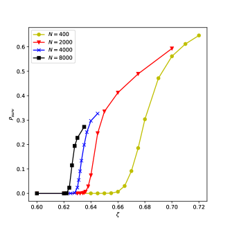
Figure 3: Estimate of the asymptotic density in the fixed-energy version of the AMM on random $5$-regular graphs of different sizes. The approximate critical point, identified as the onset of asymptotic survival, at around $\zeta_{c}=0.62$ is very close to the theoretical prediction $\zeta_{c}=1/2+1/q=0.6$.

IV Discussion

In the procedure outlined above, we have cast the dynamics of the Abelian Manna Model in a multi-type branching process, whose species consist of multiple-site motives of active sites. Upon charging a singly occupied site a branching process ensues and evolves by producing offspring according to the density of occupied sites $\zeta$. The critical density $\zeta_{c}$ of the AMM is identified with the value of $\zeta$ when the branching process is critical. Our main results Eq. (8) is in line with numerical findings in the literature, Tab. 1. The most significant corrections are found in low dimensions and almost perfect agreement in dimension $d=5$.

The multi-type branching process mapping we introduce keeps track only of the parity of active sites and the total number of particles post-toppling at their neighbours. These few motives allow us to find a closed form estimate of the critical density on regular lattices and more complicated graphs. Compared with other theoretical methods which characterise the critical density of the AMM such as real-space renormalisation group Pietronero et al. (1994); Lin (2010) and n-site approximations Dickman et al. (2002); Dickman (2002), our approach utilises only the local topology of the underlying graph, rendering it more flexible and easier to generalise. In spirit, these active motives are closely related to those in the Approximate Master Equation method Gleeson (2011, 2013) which improves significantly on a pair approximation. The treatment of the AMM activity here differs from that method by capturing mobile branching motives. To our knowledge, this has not been considered in the literature before.

The main focus of the present work is not to improve the estimates of the critical density in one dimension, which display the most significant deviation from the mean-field value. Rather, we identify the key ingredients that contribute to the deviation of the critical density from the mean-field value and characterise the deviation analytically. The AMM is believed to belong to the conserved directed percolation (CDP) universality class Vespignani et al. (2000); Rossi et al. (2000b), which is different from the more general directed percolation (DP) universality class due to the conservation of particles in the dynamics. Through the mapping of AMM avalanches to a multi-type branching process, we explicitly show that the nearest-neighbour dynamical correlations and conservation of particles during avalanching largely capture the shift of the critical density away from its mean-field value, as prescribed by a simple binary branching process.

Our mimicking process provides insight into the evolution of activity in AMM avalanches. During an avalanche, activity grows (active motives branch) at the cost of singly-occupied sites, so that the sites receiving toppling particles are occupied with a probability less than their mean density. The conservation of particles and their spatial correlations thus lead to local suppression of branching. Two phenomena are ignored in our mapping of the AMM. Firstly, the total number of particles in the system during avalanching may be reduced due to dissipation at open boundaries, and the number of singly occupied sites may decrease because of this as well as because of growing activity. As a result, branching is suppressed globally, yet this effect is weak, as only a few sites are affected Willis and Pruessner (2018b). Secondly, We ignore long-ranged anti-correlations Basu et al. (2012); Hexner and Levine (2015) in the quiescent state of the AMM, which, however, appear to be rather weak albeit algebraic Willis and Pruessner (2018b). Building on the mapping we construct here, it would be interesting for future work to establish a rigorous lower bound of the critical density in the AMM by associating the activity with some critical population dynamics, for example via the coupling method Lindvall (2002); Levin and Peres (2017).