Cross validation for penalized quantile regression with a case-weight adjusted solution path

Abstract

Cross validation is widely used for selecting tuning parameters in regularization methods, but it is computationally intensive in general. To lessen its computational burden, approximation schemes such as generalized approximate cross validation (GACV) are often employed. However, such approximations may not work well when non-smooth loss functions are involved. As a case in point, approximate cross validation schemes for penalized quantile regression do not work well for extreme quantiles. In this paper, we propose a new algorithm to compute the leave-one-out cross validation scores exactly for quantile regression with ridge penalty through a case-weight adjusted solution path. Resorting to the homotopy technique in optimization, we introduce a case weight for each individual data point as a continuous embedding parameter and decrease the weight gradually from one to zero to link the estimators based on the full data and those with a case deleted. This allows us to design a solution path algorithm to compute all leave-one-out estimators very efficiently from the full-data solution. We show that the case-weight adjusted solution path is piecewise linear in the weight parameter, and using the solution path, we examine case influences comprehensively and observe that different modes of case influences emerge, depending on the specified quantiles, data dimensions and penalty parameter.

1 Introduction

With the rapid growth of data dimensionality, regularization is widely used in model estimation and prediction. In penalized regression methods such as LASSO and ridge regression, the penalty parameter plays an essential role in determining the trade-off between bias and variance of the corresponding regression estimator. Too large a penalty could lead to undesirably large bias while too small a penalty would lead to instability in the estimator. The penalty parameter can be chosen to minimize the prediction error associated with the estimator. Cross validation (CV) (Stone, 1974) is the most commonly used technique for choosing the penalty parameter based on data-driven estimates of the prediction error, especially when there is not enough data available.

Typically, fold-wise CV is employed in practice. When the number of folds is the same as the sample size, it is known as leave-one-out (LOO) CV. For small data sets, LOO CV provides approximately unbiased estimates of the prediction error while the general $k$-fold CV may produce substantial bias due to the difference in sample size for the fold-wise training data and the original data (Kohavi, 1995). Moreover, for linear modeling procedures such as smoothing splines, the fitted values from the full data can be explicitly related to the predicted values for LOO CV (Craven and Wahba, 1979). Thus, the LOO CV scores are readily available from the full data fit. The linearity of a modeling procedure that enables exact LOO CV is strongly tied to squared error loss employed for the procedure and the simplicity of the corresponding optimality condition for the solution.

However, loss functions for general modeling procedures may not yield such simple optimality conditions as squared error loss does, and result in more complex relation between the fitted values and the observed responses. In general, the LOO predicted values may not be related to the full data fit in closed form. Consequently, the computation needed for LOO CV becomes generally intensive as LOO prediction has to be made for each of $n$ cases separately given each candidate penalty parameter.

In this paper we focus on LOO CV for penalized M-estimation with nonsmooth loss functions, in particular, quantile regression with ridge penalty (QRRP). Quantile regression (Koenker and Bassett, 1978) can provide a comprehensive description of the conditional distribution of the response variable given a set of covariates, and it has become an increasingly popular tool to explore the data heterogeneity (Koenker, 2017). Extreme quantiles can also be used for outlier detection (Chaouch and Goga, 2010). Penalized quantile regression is specifically suited for analysis of high-dimensional heterogeneous data.

The check loss for quantile regression with a pre-specified quantile parameter $\tau\in(0,1)$ is defined as

$$\rho_{\tau}(r)=\tau r_{+}+(1-\tau)(-r)_{+},\text{ where }r_{+}=\max(r,0).$$ (1)

Unlike squared error loss, the check loss is nondifferentiable at 0 as is shown in Figure 1.

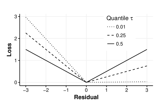
Figure 1: The check loss for quantile regression with quantile parameter $\tau=0.01,\leavevmode\nobreak\ 0.25\text{ and }0.5$

To lessen the computational cost of the exact LOO CV in this setting, Nychka et al. (1995) and Yuan (2006) proposed Approximate CV (ACV) and Generalized Approximate CV (GACV). Using a smooth approximation of the check loss, they applied similar arguments used in mean regression for the derivation of ordinary cross validation (OCV) (Allen, 1971) and generalized cross validation (GCV) (Wahba et al., 1979) to quantile regression. The key ingredients for the arguments are the leave-one-out lemma (see Section 3.2) and the first-order Taylor expansion of the smoothed check loss. The linearization error from the first-order Taylor expansion may not be ignorable for extreme quantiles due to the increasing skewness of the distribution of the LOO residuals that is at odds with the increase in the slope of the check loss with $\tau$ (see Section 4.1.1 for details). This phenomenon can be easily illustrated. Figure 2 compares the exact LOO CV and GACV scores as a function of the penalty parameter $\lambda$ for various quantiles in a simulation setting (see Section 4 for details). For instance, the approximate CV scores in the figure could produce penalty parameter values that are very different from the exact LOO CV when $\tau=0.01$ and $0.1$. The empirical studies in Li et al. (2007) and Reiss and Huang (2012) also confirm the inaccuracy of the approximation for extreme quantiles. This result motivates us to explore other computationally efficient schemes for exact LOO CV.

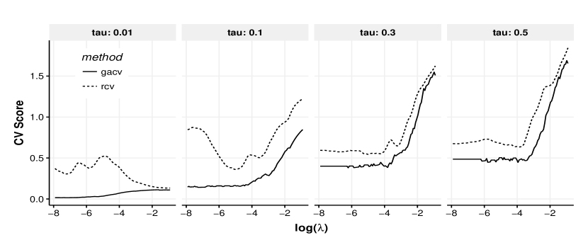
Figure 2: Comparison of the exact LOO CV and GACV scores for penalized quantile regression ($\tau=0.01,\leavevmode\nobreak\ 0.1,\leavevmode\nobreak\ 0.3,\text{ and }0.5$). The exact LOO CV score is defined as $RCV(\lambda)=\frac{1}{n}\sum_{i=1}^{n}\rho_{\tau}\big{(}y_{i}-\hat{f}_{\lambda}^{[-i]}(x_{i})\big{)}$, and GACV score from Li et al. (2007) is defined as $GACV(\lambda)=\frac{1}{n-|\mathcal{E}_{\lambda}|}\sum_{i=1}^{n}\rho_{\tau}(y_{i}-\hat{f}(x_{i}))$.

Instead of treating $n$ LOO problems separately, we exploit the homotopy strategy to relate them to the full-data problem. The $n$ LOO problems can be viewed as perturbations of the full-data problem. The key idea of homotopy is to start from a problem with known solution and gradually adjust the problem with respect to a continuous homotopy parameter until we reach the desired target problem and its solution. In our approach, we leverage the full-data solution as a starting point for the LOO problems. In optimization, homotopy techniques have been used in many algorithms including the interior point algorithm derived from perturbed KKT conditions (Zhao et al., 2012) and parametric active set programming (Allgower and Georg, 1993). In statistical learning community, the latter has been widely used in the form of path-following algorithms. For instance, Osborne (1992) and Osborne et al. (2000) apply the homotopy technique to generate piecewise linear trajectories in quantile regression and LASSO problems, respectively. Later Efron et al. (2004), Hastie et al. (2004) and Rosset and Zhu (2007) exploit the homotopy path-following methods to generate an entire solution path for a family of regularization problems indexed by the penalty parameter.

In this paper, we propose an exact path-following algorithm for LOO cross validation in penalized quantile regression by introducing a case-weight $\omega$ for the held-out case as a continuous homotopy parameter. We vary the case-weight $\omega$ from 1 to 0 to link the full-data setting to the LOO setting. Let $\{(x_{i},y_{i})\}_{i=1}^{n}$ be the full data with covariates $x_{i}\in\mathbb{R}^{p}$ and response $y_{i}\in\mathbb{R}$. Given fixed quantile $\tau$ and penalty parameter $\lambda$, for each case $i^{\star}\in\{1,\cdots,n\}$, consider the following case-weight adjusted quantile regression problem with linear regression quantiles:

$$\operatorname*{minimize\,}_{\beta_{0}\in\mathbb{R},{\beta}\in\mathbb{R}^{p}}\sum_{i\neq i^{\star}}\rho_{\tau}(y_{i}-\beta_{0}-x_{i}^{\top}{\beta})+\omega\rho_{\tau}(y_{i^{\star}}-\beta_{0}-x_{i^{\star}}^{\top}{\beta})+\frac{\lambda}{2}\|\beta\|_{2}^{2}.$$ (2)

The problem in (2) with $\omega=1$ involves the full data while $\omega=0$ leaves out the case $i^{\star}$. By decreasing the case weight $\omega$ from 1 to 0, we successfully link the two separate but intrinsically related problems. Notice that the full data solution needs to be computed only once and can be used repeatedly as a starting point for $n$ LOO problems. We provide an efficient homotopy algorithm to generate the solution path indexed by $\omega$, which results in the LOO solution. Hence, with the LOO solutions, we can compute CV scores exactly, circumventing the issues with approximate CV especially for extreme quantiles.

There have been many works on computation of the solution paths for penalized quantile regression. In spirit of Hastie et al. (2004), Li and Zhu (2008) and Li et al. (2007) proposed algorithms for solution paths in $\lambda$ given quantile $\tau$ in $l_{1}$-penalized quantile regression and kernel quantile regression, respectively. By varying quantile parameter $\tau$, Takeuchi et al. (2009) examined the solution path as a function of $\tau$ for fixed $\lambda$ in kernel quantile regression. Further, Rosset (2009) developed an algorithm for a generalized bi-level solution path as a function of both $\lambda$ and $\tau$. These algorithms are driven by a set of optimality conditions that imply piecewise linearity of the solution paths. Due to the linear structure in the additional term with a case-weight $\omega$ in (2), it can be shown that the case-weight adjusted solution path is also piecewise linear in $\omega$. This piecewise linearity allows us to devise a new path-following algorithm, which starts from the full-data solution and reaches the LOO solution at the end. We derive the optimality conditions for the case-weight adjusted solution and provide a formal proof that solutions from the algorithm satisfy the KKT conditions at every $\omega\in[0,1]$.

The proposed path-following algorithm with a varying case-weight $\omega$ does not only offer the LOO solutions efficiently, but also provides case influence measures and a new way of approximating the model degrees of freedom. We demonstrate numerically and analytically that the computational cost of the proposed algorithm in evaluation of LOO CV scores could be much lower than that of a simple competing method. This also allows an efficient evaluation of the influence of the case on the fitted model as a function of $\omega$. Different from case-deletion diagnostics (Cook, 1977; Belsley et al., 1980), Cook (1986) proposed analogous case influence graphs to assess local influence of a statistical model. Using the case-weight adjusted solution path, we can generate case influence graphs efficiently for penalized quantile regression and examine the influence of small perturbations of data on regression quantiles. In contrast to mean regression, it is observed that cases with almost identical case deletion statistics could have quite different case influence graphs in quantile regression. In addition, we generalize the leave-one-out lemma by considering a data perturbation scheme that is more general than case deletion and naturally associated with the case weight adjustment. Using the generalized lemma, we propose a new approach to approximating model degrees of freedom based on the case-weight adjusted solutions. Numerically, we observe that data dimension and penalty parameter value can influence the computational time of the algorithm.

The paper is organized as follows. Section 2 proposes a path-following algorithm for case-weight adjusted quantile regression with ridge penalty for cross validation. A formal validation of the algorithm is provided on the basis of the optimality conditions. Section 3 presents another application of the case-weight adjusted solutions for measuring case influence on regression quantiles and approximating the model degrees of freedom. In Section 4, some numerical studies are presented to illustrate the applications of the proposed case-weight adjusted solution path algorithm and its favorable computational efficiency for computing LOO CV scores. We conclude with some remarks in Section 5. Technical proofs are provided in Appendix.

2 Case-weight Adjusted Solution Path in Quantile Regression with Ridge Penalty

In this section, we present a path-following algorithm for solving the penalized quantile regression problem in (2) with case weight $\omega$. We illustrate in detail how to construct a solution path from the full-data solution as the case weight decreases from $1$ to $0$. As with many existing solution path algorithms, the key to our derivations is the optimality conditions for (2). We analyze the Karush-Kuhn-Tucker (KKT) conditions for the problem after reformulating it as a constrained optimization problem. We formally prove that the path generated by the proposed algorithm solves the problem (2), and is piecewise linear in $\omega$.

2.1 Optimality Conditions

In the path-following algorithm, we start from the full-data solution at $\omega=1$, and specify a scheme to update the solution as $\omega$ decreases from $1$ to $0$. The updating scheme is designed so that the path generated satisfies the KKT conditions for every $\omega$ in $[0,1]$. As such, we first derive the KKT conditions for the optimization problem (2). Toward this end, let $(\beta_{0,\omega},\beta_{\omega})$ denote the solution of (2). By (1) and the fact that $\max(x,0)=\inf_{t\geq 0,t\geq x}t$, we introduce auxiliary variables $\xi=(\xi_{1},\cdots,\xi_{n})$ and $\zeta=(\zeta_{1},\cdots,\zeta_{n})$ with $\xi_{i}\geq\max(y_{i}-\beta_{0}-x_{i}^{\top}\beta,0)$ and $\zeta_{i}\geq\max(-(y_{i}-\beta_{0}-x_{i}^{\top}\beta),0)$ for $i=1,\ldots,n$ to reexpress the check loss as follows:

$$\rho_{\tau}(y_{i}-\beta_{0}-x_{i}^{\top}\beta) = \tau\max(y_{i}-\beta_{0}-x_{i}^{\top}\beta,0)+(1-\tau)\max(-(y_{i}-\beta_{0}-x_{i}^{\top}\beta),0)$$

$$= \inf_{\xi_{i},\zeta_{i}\geq 0\text{ and }-\zeta_{i}\leq y_{i}-\beta_{0}-x_{i}^{\top}\beta\leq\xi_{i}}\tau\xi_{i}+(1-\tau)\zeta_{i}\,.$$

Thus, we can rewrite the optimization problem (2) as

$$\begin{array}[]{cl}\underset{\beta_{0}\in\mathbb{R},\beta\in\mathbb{R}^{p},\xi\in\mathbb{R}^{n},\zeta\in\mathbb{R}^{n}}{\operatorname*{minimize\,}}&\tau\sum_{i\neq i^{\star}}\xi_{i}+(1-\tau)\sum_{i\neq i^{\star}}\zeta_{i}+\omega\tau\xi_{i^{\star}}+\omega(1-\tau)\zeta_{i^{\star}}+\frac{\lambda}{2}\|\beta\|_{2}^{2}\\ \text{subject to }&-\zeta_{i}\leq y_{i}-\beta_{0}-x_{i}^{\top}\beta\leq\xi_{i},\text{and }\zeta_{i},\xi_{i}\geq 0\text{ for }i=1,\cdots,n\,.\end{array}$$ (3)

Note that (3) is in the standard form of a constrained convex optimization problem:

$$\begin{array}[]{cl}\underset{x\in\mathbb{R}^{n}}{\operatorname*{minimize\,}}&f(x)\\ \text{ subject to }&g_{i}(x)\leq 0\text{ for }i=1,\ldots,m\,,\end{array}$$ (4)

where $f(\cdot)$ and $g_{i}(\cdot)$ are convex functions. It is well-known that the KKT conditions for (4) are

$$\begin{array}[]{ll}\nabla f(x)+\sum_{i=1}^{m}\lambda_{i}\nabla g_{i}(x)=0\,,\text{ and }\\ \lambda_{i}g_{i}(x)=0,\quad\text{ for some real numbers }\lambda_{i}\geq 0,\leavevmode\nobreak\ i=1,\ldots,m\,.\end{array}$$ (5)

By letting $x=(\beta_{0},\beta,\xi,\zeta)$, $g_{i}(x)=-\zeta_{i}$, $g_{n+i}(x)=-\xi_{i}$, $g_{i+2n}(x)=\beta_{0}+x_{i}^{\top}\beta-y_{i}-\zeta_{i}$, and $g_{i+3n}(x)=y_{i}-\beta_{0}-x_{i}^{\top}\beta-\xi_{i}$ for $i=1,\ldots,n$, we can write, after some simplifications, the KKT conditions for (3) as

$$X^{\top}\theta_{\omega}=\lambda\beta_{\omega}\,,\text{ and }\,\theta_{\omega}^{\top}{1}=0$$ (6)

$$\theta_{i,\omega}=\begin{cases}\tau-1&\text{ for }i\neq i^{\star}\\ \omega(\tau-1)&\text{ for }i=i^{\star}\end{cases} \text{if }y_{i}-\beta_{0,\omega}-x_{i}^{\top}\beta_{\omega}<0$$ (7)

$$\theta_{i,\omega}\in\begin{cases}[\tau-1,\tau]&\text{ for }i\neq i^{\star}\\ [\omega(\tau-1),\omega\tau]&\text{ for }i=i^{\star}\end{cases} \text{if }y_{i}-\beta_{0,\omega}-x_{i}^{\top}\beta_{\omega}=0$$ (8)

$$\theta_{i,\omega}=\begin{cases}\tau&\text{ for }i\neq i^{\star}\\ \omega\tau&\text{ for }i=i^{\star}\end{cases} \text{if }y_{i}-\beta_{0,\omega}-x_{i}^{\top}\beta_{\omega}>0$$ (9)

where $\theta_{\omega}=(\theta_{1,\omega},\ldots,\theta_{n,\omega})\in\mathbb{R}^{n}$ is the set of dual variables associated with the residual bounds and $X=\begin{pmatrix}x_{1}^{\top}\\ \vdots\\ x_{n}^{\top}\end{pmatrix}$ is the $n\times p$ design matrix. A detailed derivation is included in the Appendix A.1. The solution $(\beta_{0,\omega},\beta_{\omega})$ and $\theta_{\omega}$ can thus be determined by the equality conditions in (6)–(9).

2.2 Outline of the Solution Path Algorithm

Let $r_{i,\omega}=y_{i}-\beta_{0,\omega}-x_{i}^{\top}\beta_{\omega}$ denote the residual for the $i$th case with $(\beta_{0,\omega},\beta_{\omega})$. According to the sign of each residual, we can partition the $n$ cases into three sets. Depending on which side of $0$ each residual falls on, the three sets are called the elbow set, $\mathcal{E_{\omega}}=\{i:r_{i,\omega}=0\}$, the left set of the elbow, $\mathcal{L_{\omega}}=\{i:r_{i,\omega}<0\}$ and the right set of the elbow, $\mathcal{R_{\omega}}=\{i:r_{i,\omega}>0\}$. The three sets may evolve as $\omega$ decreases. We call $\omega_{m}$ a breakpoint if the three sets change at $\omega_{m}$. The following rules specify how and when we should update the three sets at each breakpoint:

1. if $\theta_{i,\omega}$ = $\tau[\omega+(1-\omega)\mathbb{I}(i\neq i^{\star})]$ for some $i\in\mathcal{E_{\omega}}$, then move case $i$ from $\mathcal{E_{\omega}}$ to the right set of the elbow $\mathcal{R_{\omega}}$.

2. if $\theta_{i,\omega}$ = $(\tau-1)[\omega+(1-\omega)\mathbb{I}(i\neq i^{\star})]$ for some $i\in\mathcal{E_{\omega}}$, then move case $i$ from $\mathcal{E_{\omega}}$ to the left set of the elbow $\mathcal{L_{\omega}}$.

3. if $r_{i,\omega}=0$ for some $i\in\mathcal{L_{\omega}}\cup\mathcal{R_{\omega}}$, then move case $i$ from $\mathcal{L_{\omega}}\cup\mathcal{R_{\omega}}$ to the elbow set $\mathcal{E_{\omega}}$.

Figure 3: Change in the three sets from $(\mathcal{L}_{m-1},\mathcal{E}_{m-1},\mathcal{R}_{m-1})$ to $(\mathcal{L}_{m},\mathcal{E}_{m},\mathcal{R}_{m})$ at $\omega_{m}$.

Given the three sets, we next analyze how the solution should evolve between two breakpoints. Toward this end, we let $\{\omega_{i},\text{ for }i=0,1,\ldots,M\mid 0\leq\omega_{M}<\cdots<\omega_{1}<\omega_{0}=1\}$ be the set of breakpoints, and denote by $\mathcal{E}_{m}$, $\mathcal{L}_{m}$ and $\mathcal{R}_{m}$ the three sets between $\omega_{m+1}$ and $\omega_{m}$ for $m=1,\ldots,M$ (see Figure 3). Now, when $\omega_{m+1}<\omega<\omega_{m}$, the KKT conditions determine how $(\beta_{0,\omega},\beta_{\omega})$ and $\theta_{\omega}$ should change as functions of $\omega$ and we can show that they satisfy the following:

$$\begin{array}[]{clc}-\sum_{i\in\mathcal{E}_{m}}\theta_{i,\omega}&=&\sum_{i\notin\mathcal{E}_{m}}\theta_{i,\omega}\\[4.30554pt] \lambda\beta_{\omega}-\sum_{i\in\mathcal{E}_{m}}\theta_{i,\omega}x_{i}&=&\sum_{i\notin\mathcal{E}_{m}}\theta_{i,\omega}x_{i}\\[4.30554pt] \beta_{0,\omega}+x_{i}^{\top}\beta_{\omega}&=&y_{i}\quad\text{ for }i\in\mathcal{E}_{m}\end{array}$$ (10)

using (6) and (8), and the fact that $\theta_{i,\omega}=\{\tau-\mathbb{I}(i\in\mathcal{L}_{m})\}\{\omega+(1-\omega)\mathbb{I}(i\neq i^{\star})\}$ for $i\notin\mathcal{E}_{m}$ from (7) and (9).

Next, we show that $(\beta_{0,\omega},\beta_{\omega},\theta_{\omega})$ satisfying (10) must be linear in $\omega$. Before proceeding, we introduce some notations. For any vector $v=(v_{1},\ldots,v_{n})^{\top}\in\mathbb{R}^{n}$ and any index set $A=\{i_{1},\ldots,i_{k}\}\subseteq\{1,2,\ldots,n\}$, define $v_{A}=(v_{i_{1}},\ldots,v_{i_{k}})$ be a sub-vector of $v$. Similarly, for any matrix $M=\begin{pmatrix}m_{1}^{\top}\\ \vdots\\ m_{n}^{\top}\end{pmatrix}\in\mathbb{R}^{n\times L}$, let $M_{A}=\begin{pmatrix}m_{i_{1}}^{\top}\\ \vdots\\ m_{i_{k}}^{\top}\end{pmatrix}$ be a submatrix of $M$, where $m_{i}^{\top}$ is the $i$th row of $M$ for $i=1,\ldots,n$. Let $\mathbf{1}$ be the vector of ones and $\mathbf{0}$ be the matrix of zeros of appropriate size. Now we can rewrite (10) into a matrix form:

$$\begin{pmatrix}0&\mathbf{0}^{\top}_{p}&-{\mathbf{1}}^{\top}_{\mathcal{E}_{m}}\\[4.30554pt] 0&\lambda I_{p\times p}&-X^{\top}_{\mathcal{E}_{m}}\\ {\mathbf{1}}_{\mathcal{E}_{m}}&X_{\mathcal{E}_{m}}&\mathbf{0}_{\mathcal{E}_{m}}\end{pmatrix}\begin{pmatrix}\beta_{0,\omega}\\[4.30554pt] \beta_{\omega}\\ \theta_{{\mathcal{E}_{m}},\omega}\end{pmatrix}=\begin{pmatrix}{\mathbf{1}}^{\top}_{\mathcal{L}_{m}}\theta_{\mathcal{L}_{m}}+{\mathbf{1}}^{\top}_{\mathcal{R}_{m}}\theta_{\mathcal{R}_{m}}\\[4.30554pt] X^{\top}_{\mathcal{L}_{m}}\theta_{\mathcal{L}_{m}}+X^{\top}_{\mathcal{R}_{m}}\theta_{\mathcal{R}_{m}}\\ y_{\mathcal{E}_{m}}\end{pmatrix}$$

which is a system of linear equations of dimension $1+p+|\mathcal{E}_{m}|$. Note that the left hand side of the above linear equation does not depend on $\omega$, while the right hand side is a linear function of $\omega$. This implies that its solution must be a linear function of $\omega$. The following lemma summarizes the properties of the solution path described thus far.

Lemma 1.

The solution path $(\beta_{0,\omega},\beta_{\omega})$ satisfying the KKT conditions (6)–(9) is piecewise linear in $\omega$.

Using Lemma 1, we propose a solution path algorithm that updates the three sets following the aforementioned rules at each breakpoint and linearly updates the solutions between two consecutive breakpoints. First we provide an outline of our algorithm:

• Start with the full-data solution at $\omega=1$.

• While $\omega>0$,

  1. Decrease $\omega$ and update $(\beta_{0,\omega},\beta_{\omega})$ and $\theta_{\omega}$ until one of the inequalities in the KKT conditions is violated.

  2. When the violation happens, update the three sets according to the rules (a)–(c). Then go back to Step (i).

2.3 Determining Breakpoints

For implementation of Step (i), we need to derive a formula for the next breakpoint $\omega_{m+1}$ among $\omega\leq\omega_{m}$. From the KKT conditions (6)–(9), we can see that as $\omega$ decreases, the conditions (7)–(9) will be violated when $\theta_{i,\omega}=\tau[\omega+(1-\omega)\mathbb{I}(i\neq i^{\star})]\text{ or }(\tau-1)[\omega+(1-\omega)\mathbb{I}(i\neq i^{\star})]$ for some $i\in\mathcal{E}_{m}$, or $r_{i,\omega}=0$ for some $i\in\mathcal{L}_{m}\cup\mathcal{R}_{m}$. Thus, to find the next breakpoint $\omega_{m+1}$, we need to derive how $\theta_{{\mathcal{E}_{m}},\omega}$ and $r_{\omega}=(r_{1,\omega},\ldots,r_{n,\omega})$ change as functions of $\omega$. This is established in the following proposition, for which we need to impose an assumption that any $\min(p+2,n)$ points of $\{(\tilde{x}_{i},y_{i})\}^{n}_{i=1}$ are linearly independent, where $\tilde{x}_{i}=(1,x_{i}^{\top})^{\top}$. We call this condition the general position condition. A similar condition is also imposed in Li et al. (2007).

Proposition 1.

Suppose that the data points $\{(\tilde{x}_{i},y_{i})\}_{i=1}^{n}$ satisfy the general position condition. Then the solution path for (2) satisfies the following properties:

• When $i^{\star}\in\mathcal{R}_{m}\cup\mathcal{L}_{m}$, we have that

  $$\theta_{\mathcal{E}_{m},\omega}-\theta_{\mathcal{E}_{m},\omega_{m}}=b_{m}(\omega-\omega_{m})\,,$$ (11)

  where

  $$b_{m} = -(\tilde{X}_{\mathcal{E}_{m}}\tilde{X}_{\mathcal{E}_{m}}^{\top})^{-1}\left[b_{0,m}1_{\mathcal{E}_{m}}+\tilde{X}_{\mathcal{E}_{m}}\tilde{x}_{i^{\star}}(\tau-\mathbb{I}(i^{\star}\in\mathcal{L}_{m}))\right]$$ (12)

  with $$b_{0,m}=\frac{1-1_{\mathcal{E}_{m}}^{\top}(\tilde{X}_{\mathcal{E}_{m}}\tilde{X}_{\mathcal{E}_{m}}^{\top})^{-1}\tilde{X}_{\mathcal{E}_{m}}\tilde{x}_{i^{\star}}}{1_{\mathcal{E}_{m}}^{\top}(\tilde{X}_{\mathcal{E}_{m}}\tilde{X}_{\mathcal{E}_{m}}^{\top})^{-1}1_{\mathcal{E}_{m}}}(\tau-\mathbb{I}(i^{\star}\in\mathcal{L}_{m}))\,,$$ (13)

  and

  $$\lambda(r_{\omega}-r_{\omega_{m}})=h_{m}(\omega-\omega_{m})\,,$$ (14)

  where

  $$h_{m}=-b_{0,m}{1}-\tilde{X}\left[\tilde{X}_{\mathcal{E}_{m}}^{\top}b_{m}+\{\tau-\mathbb{I}(i^{\star}\in\mathcal{L}_{m})\}\tilde{x}_{i^{\star}}\right]\,.$$ (15)

• Moreover, $i^{\star}\in\mathcal{E}_{m}$ can only happen when $m=0$, and if that happens, both $r_{\omega}$ and $\theta_{\omega}$ are constant vectors for $\omega\in[\omega_{1},1]$, and $i^{\star}$ will move from $\mathcal{E}_{0}$ to $\mathcal{L}_{1}\cup\mathcal{R}_{1}$ at the next breakpoint $\omega_{1}=\frac{{\theta}_{i^{\star},\omega_{0}}}{\tau-\mathbb{I}({\theta}_{i^{\star},\omega_{0}}<0)}$, and stay in $\mathcal{L}_{m}\cup\mathcal{R}_{m}$ for all $m=1,\ldots,M$.

The proof of Proposition 1 is provided in the Appendix. Using Proposition 1, we can easily determine the next breakpoint if $i^{\star}\in\mathcal{L}_{m}\cup\mathcal{R}_{m}$. Specifically, the next breakpoint is determined by the largest $\omega<\omega_{m}$ such that $\theta_{i,\omega}=\tau\text{ or }\tau-1$ for some $i\in\mathcal{E}_{m}$, or $r_{i,\omega}=0$ for some $i\in\mathcal{L}_{m}\cup\mathcal{R}_{m}$. Hence, the next breakpoint is

$$\omega_{m+1}=\max(\omega_{1,m+1},\omega_{2,m+1})\,,$$ (16)

where $\omega_{1,m+1}$ is the largest $\omega<\omega_{m}$, at which $\theta_{i,\omega}$, for some $i\in\mathcal{E}_{m}$, hits either of the boundaries $\tau$ or $\tau-1$, and $\omega_{2,m+1}$ is the largest $\omega<\omega_{m}$, at which $r_{i,\omega}$ hits $0$ for some $i\in\mathcal{L}_{m}\cup\mathcal{R}_{m}$. Moreover, we know that $\theta_{\mathcal{E}_{m},\omega}$ and $r_{\omega}$ evolve as linear functions of $\omega$ according to (11) and (14), from which we obtain the following for $\omega_{1,m+1}$ and $\omega_{2,m+1}$:

$$\omega_{1,m+1} =\underset{\theta\in\{\tau,\tau-1\}}{\max}\left(\underset{i\in\mathcal{E}_{m}\text{ and }-\omega_{m}\leq\frac{\theta-\theta_{i,\omega_{m}}}{b_{i,m}}<0}{\max}\frac{\theta-\theta_{i,\omega_{m}}}{b_{i,m}}+\omega_{m}\right)$$ (17a)

$$\omega_{2,m+1} =\underset{i\in\mathcal{L}_{m}\cup\mathcal{R}_{m}\text{ and }0<\frac{\lambda r_{i,\omega_{m}}}{h_{i,m}}\leq\omega_{m}}{\max}-\frac{\lambda r_{i,\omega_{m}}}{h_{i,m}}+\omega_{m}\,,$$ (17b)

where $b_{i,m}$ and $h_{i,m}$ are the $i$th component of slopes $b_{m}$ and $h_{m}$ defined in (12) and (15), respectively. From these two formulas, we can see that the next breakpoint can be determined without evaluating the solutions between two breakpoints.

2.4 A Path-Following Algorithm

We summarize the detailed description of our proposed solution-path algorithm in Algorithm 1.

1 Input:  $X\in\mathbb{R}^{n\times p},y\in\mathbb{R}^{n},\tau\in(0,1),{\lambda}\in\mathbb{R}^{+},i^{\star}\in\{1,\cdots,n\},\hat{\beta}_{0,\omega_{0}},\hat{\beta}_{\omega_{0}}$

2 Set $\mathcal{L}_{0}=\{i:y_{i}-\hat{\beta}_{0,\omega_{0}}-x_{i}^{\top}\hat{\beta}_{\omega_{0}}<0\}$, $\mathcal{E}_{0}=\{i:y_{i}-\hat{\beta}_{0,\omega_{0}}-x_{i}^{\top}\hat{\beta}_{\omega_{0}}=0\}$, $\mathcal{R}_{0}=\{i:y_{i}-\hat{\beta}_{0,\omega_{0}}-x_{i}^{\top}\hat{\beta}_{\omega_{0}}>0\}$.

3 Compute $\hat{\theta}_{\omega_{0}}$ by setting $\hat{\theta}_{\mathcal{L}_{0},\omega_{0}}=(\tau-1)\mathbf{1}$, $\hat{\theta}_{\mathcal{R}_{0},\omega_{0}}=\tau\mathbf{1}$, and $\hat{\theta}_{\mathcal{E}_{0},\omega_{0}}=(\tilde{X}_{\mathcal{E}_{0}}\tilde{X}_{\mathcal{E}_{0}}^{\top})^{-1}\big{[}\lambda y_{\mathcal{E}_{0}}-\lambda\hat{\beta}_{0,\omega_{0}}{1}_{\mathcal{E}_{0}}-\tilde{X}_{\mathcal{E}_{0}}\big{(}\tilde{X}^{\top}_{\mathcal{L}_{0}}\hat{\theta}_{\mathcal{L}_{0},\omega_{0}}+\tilde{X}^{\top}_{\mathcal{R}_{0}}\hat{\theta}_{\mathcal{R}_{0},\omega_{0}}\big{)}\big{]}$ (see (33));

4 Set $m=0$;

5

6if $i^{\star}\in\mathcal{E}_{0}$ then

7       $\omega_{\text{1}}=\frac{\hat{\theta}_{i^{\star},\omega_{0}}}{\tau-\mathbb{I}(\hat{\theta}_{i^{\star},\omega_{0}}<0)}$;

8       Set $(\hat{\beta}_{\omega},\hat{\beta}_{0,\omega},\hat{\theta}_{\omega})=(\hat{\beta}_{\omega_{0}},\hat{\beta}_{0,\omega_{0}},\hat{\theta}_{\omega_{0}})$ for any $\omega\in[\omega_{1},1]$;

9       if $\omega_{1}>0$ then

10             Update the three sets: $(\mathcal{L}_{1},\mathcal{E}_{1},\mathcal{R}_{1})=(\mathcal{L}_{0},\mathcal{E}_{0}\setminus\{i^{\star}\},\mathcal{R}_{0}\cup\{i^{\star}\})$ if $\hat{\theta}_{i^{\star},\omega_{0}}>0$,

11             otherwise $(\mathcal{L}_{1},\mathcal{E}_{1},\mathcal{R}_{1})=(\mathcal{L}_{0}\cup\{i^{\star}\},\mathcal{E}_{0}\setminus\{i^{\star}\},\mathcal{R}_{0})$;

12            

13       end if

14      $m=m+1$;

15      

16 end if

17while $\omega_{m}>0$ do

18       Compute the slopes $(b_{0,m},b_{m},h_{m})$ according to (13), (12) and (15), respectively;

19       Compute the next breakpoint $\omega_{m+1}$ and its two candidates $\omega_{1,m+1}$ and $\omega_{2,m+1}$ according to (16), (17a) and (17b);

20       For each $\omega\in[\max(\omega_{m+1},0),\omega_{m})$,                                                                                        set $(\hat{\theta}_{\mathcal{L}_{m}\setminus\{i^{\star}\},\omega},\hat{\theta}_{\mathcal{R}_{m}\setminus\{i^{\star}\},\omega},\hat{\theta}_{i^{\star},\omega})=\big{(}(\tau-1){1}_{\mathcal{L}_{m}\setminus\{i^{\star}\}},\tau{1}_{\mathcal{R}_{m}\setminus\{i^{\star}\}},\omega(\tau-\mathbb{I}(i^{\star}\in\mathcal{L}_{m}))\big{)}$, $(\lambda\hat{\beta}_{0,\omega},\hat{\theta}_{\mathcal{E}_{m},\omega})=(\lambda\hat{\beta}_{0,\omega_{m}},\hat{\theta}_{\mathcal{E}_{m},\omega_{m}})+(b_{0,m},b_{m})(\omega-\omega_{m})$ and $(\lambda\hat{\beta}_{\omega},\lambda\hat{r}_{\omega})=(\lambda\hat{\beta}_{\omega_{m}},\lambda\hat{r}_{\omega_{m}})+(X_{\mathcal{E}_{m}}^{\top}b_{m}+(\tau-\mathbb{I}(i^{\star}\in\mathcal{L}_{m}))x_{i^{\star}},h_{m})(\omega-\omega_{m})$;

21       Update the three sets:

22       if $\omega_{m+1}=\omega_{1,m+1}$ then

23             Let $i$ be the index that maximizes the objective function in (17a).                                                                                        Set $(\mathcal{L}_{m+1},\mathcal{E}_{m+1},\mathcal{R}_{m+1})=(\mathcal{L}_{m},\mathcal{E}_{m}\setminus\{i\},\mathcal{R}_{m}\cup\{i\})$ if $\hat{\theta}_{i,\omega_{m+1}}=\tau$,      Rule (a)

24             otherwise $(\mathcal{L}_{m+1},\mathcal{E}_{m+1},\mathcal{R}_{m+1})=(\mathcal{L}_{m}\cup\{i\},\mathcal{E}_{m}\setminus\{i\},\mathcal{R}_{m})$;                  Rule (b)

25      else

26             Let $i$ be the index that maximizes the objective function in (17b).                                                                                        Set $(\mathcal{L}_{m+1},\mathcal{E}_{m+1},\mathcal{R}_{m+1})=(\mathcal{L}_{m}\setminus\{i\},\mathcal{E}_{m}\cup\{i\},\mathcal{R}_{m})$ if $i\in\mathcal{L}_{m}$,

27             otherwise $(\mathcal{L}_{m+1},\mathcal{E}_{m+1},\mathcal{R}_{m+1})=(\mathcal{L}_{m},\mathcal{E}_{m}\cup\{i\},\mathcal{R}_{m}\setminus\{i\})$;                  Rule (c)

28       end if

29      $m=m+1$;

30      

31 end while

Algorithm 1 The $\omega$ Path Algorithm for Case-weight Adjusted Quantile Regression

The following theorem states that the path generated by Algorithm 1 is indeed a solution path to the optimization problem (2), provided that the data points satisfy the general position condition.

Theorem 1.

Assume that the set of data points $\{(\tilde{x}_{i},y_{i})\}^{n}_{i=1}$ satisfies the general position condition. The case-weight adjusted path generated by Algorithm 1 solves the optimization problem (2) indexed by $\omega\in[0,1]$.

3 Case Influence and Degrees of Freedom in Case-weight Adjusted Regression

In addition to model validation through LOO CV, the case-weight adjusted solution path for quantile regression can be used for assessing case influences on regression quantiles. In this section, we further explore the use of the case-weight adjusted solutions for measuring case influence and model complexity.

3.1 The Assessment of Case Influence

In statistical modeling, assessing case influence and identifying influential cases is crucial for model diagnostics. Assessment of case influence on a statistical model has been extensively studied in robust statistics literature. Seminal works on case influence assessment include Cook (1977), Cook (1979) and Cook and Weisberg (1982). As a primary example, Cook proposed the following measure, known as Cook’s distance for case $i^{\star}$:

$$D_{i^{\star}}=\frac{\sum_{i=1}^{n}(\hat{f}(x_{i})-\hat{f}^{[-i^{\star}]}(x_{i}))^{2}}{p\hat{\sigma}^{2}},$$

where $\hat{\sigma}^{2}$ is an estimate of error variance. Cook’s distance measures an aggregated effect of one single case on $n$ fitted values after that case is deleted. In other words, it compares two sets of fitted values when case $i^{\star}$ has weight $\omega=1$ and $\omega=0$. In contrast to the standard Cook’s distance, Cook (1986) also introduced the notion of a case-influence graph to get a broad view of case influence as a function of case weight $\omega$. As a general version of $D_{i^{\star}}$, a case-weight adjusted Cook’s distance is defined as

$$D_{i^{\star}}(\omega)=\frac{\sum_{i=1}^{n}(\hat{f}(x_{i})-\hat{f}_{\omega}^{i^{\star}}(x_{i}))^{2}}{p\hat{\sigma}^{2}}$$ (18)

for each $\omega\in[0,1]$, where $\hat{f}_{\omega}^{i^{\star}}$ is the fitted model when case $i^{\star}$ has weight $\omega$ and the remaining cases have weight 1. When $\omega=0$, $\hat{f}_{0}^{*}$ coincides with $\hat{f}^{[-i^{\star}]}$ and thus $D_{i^{\star}}(0)=D_{i^{\star}}$. With this generalized distance, we could examine more complex modes of case influence that may not be easily detected by Cook’s distance $D_{i^{\star}}$. Figure 4 provides an example of case-influence graphs where two cases A and B have the same Cook’s distance but obviously different influence on the model fit depending on $\omega$. Two cases A and B can be treated the same if merely assessed by $D_{i^{\star}}$, but since $D_{A}(\omega)\geq D_{B}(\omega)$ at each $\omega\in[0,1]$, case A should be treated as more influential than case B.

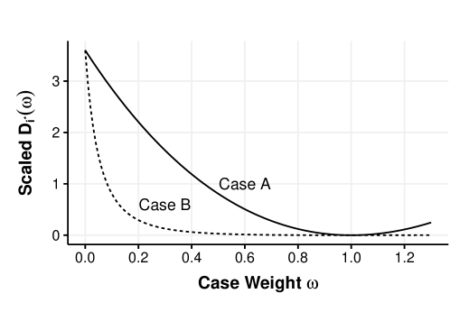
Figure 4: An illustrative example of case-influence graphs in least squares regression based on Figure 1 in Cook (1986).

Case influence graphs provide comprehensive information on local influence of cases in general, and they can be used to assess the differences in robustness of modeling procedures. But generation of such graphs is computationally more expensive than Cook’s distance. To circumvent the computational issue, Cook (1986) suggested to focus on the local influence around $\omega=1$ through the curvature of the graph. As evident in (18), once $\hat{f}_{\omega}^{i^{\star}}$ is obtained, the generalized Cook’s distance $D_{i^{\star}}(\omega)$ is readily available. Thus, using path-following algorithms that generate case-weight adjusted solutions, we can easily construct case influence graphs without additional computational cost.

Leveraging our solution path algorithm for quantile regression with adjusted case weight, we specifically study the characteristics of case-influence graphs for various quantiles. In addition, we include case influence graphs of ridge regression for comparison of mean regression and quantile regression as a robust counterpart in terms of case influences. For ridge regression with penalty parameter $\lambda$ and case weight $\omega$ for case $i^{\star}\in\{1,\cdots,n\}$, we solve the following problem:

$$\operatorname*{minimize\,}_{\beta_{0}\in\mathbb{R},{\beta}\in\mathbb{R}^{p}}\sum_{i\neq i^{\star}}(y_{i}-\beta_{0}-x_{i}^{\top}{\beta})^{2}+\omega(y_{i^{\star}}-\beta_{0}-x_{i^{\star}}^{\top}{\beta})^{2}+\lambda\|\beta\|_{2}^{2}.$$ (19)

With squared error loss, the case-weight adjusted fit $\hat{f}^{i^{\star}}_{\omega}$ can be computed in closed form and, thus, obtaining $D_{i^{\star}}(\omega)$ is straightforward for ridge regression. For quantile regression with the check loss, however, $\hat{f}^{i^{\star}}_{\omega}$ cannot be obtained as easily, but our proposed solution path algorithm readily offers the path for $D_{i^{\star}}(\omega)$ as $\omega$ decreases from 1 to 0.

We present the case-weight adjusted Cook’s distance $D_{i^{\star}}(\omega)$ for ridge regression in the following proposition. Let $H(\lambda)=\tilde{X}(\tilde{X}^{\top}\tilde{X}+\lambda\tilde{I})^{-1}\tilde{X}^{\top}$ denote the hat matrix for ridge regression with full data, where $\tilde{I}=\begin{pmatrix}0&\\ &I\end{pmatrix}$. $h_{ij}(\lambda)$ denotes the $ij$th entry of $H(\lambda)$ and $h_{ii}(\lambda)$ is the leverage of case $i$ in ridge regression.

Proposition 2.

For ridge regression with penalty parameter $\lambda$,

$$D_{i^{\star}}(\omega)=\frac{r^{2}_{i^{\star}}\sum_{j=1}^{n}h^{2}_{ji^{\star}}(\lambda)}{p\hat{\sigma}^{2}\{1/(1-\omega)-h_{i^{\star}i^{\star}}(\lambda)\}^{2}},$$ (20)

where $r_{i^{\star}}$ is the residual for case $i^{\star}$ from the full data fit.

The proposition above shows that $D_{i^{\star}}(\omega)$ for ridge regression is smooth and convex in $\omega$. The convexity comes from the fact that the second derivative of $g_{h}(\omega)=\{1/(1-\omega)-h\}^{-2}$ for a positive constant $h$ is $\{2+4h(1-\omega)\}\{1-h(1-\omega)\}^{-4}$, which is positive for $\omega\in(0,1)$. Furthermore, $g_{h}(\omega)$ with $h\in[0,1]$ decreases monotonically in $\omega\in(0,1)$ since $1/(1-\omega)$ increases in $\omega$ and $1/(1-\omega)-h>0$. This implies that as case weight $\omega$ decreases from $1$ to $0$, $D_{i^{\star}}(\omega)$ increases monotonically since $h_{i^{\star}i^{\star}}\in[0,1]$. When both $\omega=0$ and $\lambda=0$, $D_{i^{\star}}(\omega)$ reduces to standard Cook’s distance $(r^{2}_{i^{\star}}h_{i^{\star}i^{\star}})/\{p\hat{\sigma}^{2}(1-h_{i^{\star}i^{\star}})^{2}\}$, where $h_{i^{\star}i^{\star}}$ is the leverage of case $i^{\star}$ in ordinary linear regression. This can be seen from the fact that $\sum_{j=1}^{n}h^{2}_{i^{\star}j}(\lambda)$ is the $i^{\star}$th diagonal entry of $H^{2}(\lambda)$ and $H(0)$ is idempotent.

For penalized quantile regression, the piecewise linear solution path that we have constructed suggests that the discrepancy between the full-data fit and the case-weight adjusted fit at any $\omega$, $\hat{f}(x_{i})-\hat{f}_{\omega}^{i^{\star}}(x_{i})$, is also piecewise linear, and thus $D_{i^{\star}}(\omega)$ is piecewise quadratic in $\omega$. Hence, $D_{i^{\star}}(\omega)$ can be easily obtained by aggregating the piecewise squared difference in the fit from $1$ to $\omega$. Equivalently, using (15), the squared difference in the residual, $(r_{i}-r_{i,\omega})^{2}$, can be aggregated to produce $D_{i^{\star}}(\omega)$. An explicit expression of $D_{i^{\star}}(\omega)$ is provided in the proposition below.

Proposition 3.

For penalized quantile regression in (2) with penalty parameter $\lambda$, if $\omega\in(\omega_{m+1},\omega_{m}]$,

$$D_{i^{\star}}(\omega) =\frac{1}{p\hat{\sigma}^{2}}\sum_{i=1}^{n}(\hat{f}(x_{i})-\hat{f}_{\omega}^{i^{\star}}(x_{i}))^{2}=\frac{1}{p\hat{\sigma}^{2}}\sum_{i=1}^{n}(r_{i,\omega}-r_{i,\omega_{0}})^{2}$$

$$=\frac{1}{p\hat{\sigma}^{2}}\|\mathbf{r}_{\omega}-\mathbf{r}_{\omega_{m}}+\sum_{k=1}^{m}(\mathbf{r}_{\omega_{k}}-\mathbf{r}_{\omega_{k-1}})\|_{2}^{2}$$

$$=\frac{1}{p\hat{\sigma}^{2}}\|(\omega-\omega_{m})\mathbf{h}_{m}+\sum_{k=1}^{m}(\omega_{k}-\omega_{k-1})\mathbf{h}_{k-1}\|_{2}^{2}\,,$$ (21)

where $\mathbf{h}_{k}$ is the vector of the slopes of the case-weight adjusted residuals $\mathbf{r}$ over $(\omega_{k+1},\omega_{k}]$.

Numerical examples of case-influence graphs for ridge regression and quantile regression are presented in Section 4.

3.2 Effective Model Degrees of Freedom

In this section, we examine another application of a case-weight adjusted solution in approximating the model degrees of freedom of a general modeling procedure $\hat{f}$. Ye (1998) defined the effective model degrees of freedom of $\hat{f}$ in regression as

$$df(\hat{f})=\sum_{i=1}^{n}\frac{\partial\hat{f}(x_{i})}{\partial y_{i}},$$ (22)

where the fitted model $\hat{f}$ is based on data from a general regression model $y_{i}=f(x_{i})+\epsilon_{i}$. The definition above indicates the overall sensitivity of the fitted values to the perturbation of the responses as a measure of model complexity, which is generally expected to be larger for more complex modeling procedures.

According to (22), the model degrees of freedom can be evaluated exactly only when the fitted values are expressed analytically as a function of data. In general, $\frac{\partial\hat{f}(x_{i})}{\partial y_{i}}$ needs to be approximated. For complex modeling procedures such as regression trees, Ye (1998) suggested to approximate the effective model degrees of freedom by repeatedly generating perturbed data, fitting a model to the data and estimating the rate of change in the fitted values. As an alternative, using case-weight adjusted solutions, we propose a simple scheme for data perturbation which allows for approximation of the model degrees of freedom without generating any new data. The idea is inspired by the leave-one-out lemma in Craven and Wahba (1979), which describes the identity of the leave-one-out solution and the solution to perturbed data where the response of one case is replaced with its predicted value from the leave-one-out solution for smoothing splines. As a result, the lemma suggests the following approximation:

$$\frac{\partial\hat{f}(x_{i})}{\partial y_{i}}\approx\frac{\hat{f}(x_{i})-\hat{f}^{[-i]}(x_{i})}{y_{i}-\hat{f}^{[-i]}(x_{i})}.$$ (23)

This approximation becomes exact, in fact, for linear modeling procedures such as ridge regression and smoothing splines. Here we extend the leave-one-out lemma by considering a more general data perturbation scheme that changes only a fraction of a response and keeps the remaining fraction of it as it is. We call the extension under this fractional data perturbation scheme the leave-part-out lemma.

To state the extended lemma that holds true for penalized $M$-estimators in general, let $\ell(\cdot)$ be a general nonnegative loss function defined on the residual space to measure the lack of model fit and $J(f)$ be a penalty functional defined on the model space to measure the complexity of model $f$. Let $\hat{f}$ be the minimizer of the penalized empirical risk $Q(f)=\sum_{i=1}^{n}\ell(y_{i}-f(x_{i}))+\lambda J(f)$. Analogously, let $\hat{f}^{i}_{\omega}$ be the minimizer of $\sum_{j\neq i}\ell(y_{j}-f(x_{j}))+\omega\ell(y_{i}-f(x_{i}))+\lambda J(f)$ when case $i$ has weight $\omega$. For the aforementioned fractional perturbation scheme, it is natural to introduce a new response variable $\tilde{y}_{i}(\omega)$ with case weight $\omega\in[0,1]$, which takes $y_{i}$ with probability $\omega$ and $\hat{f}^{i}_{\omega}(x_{i})$ with probability $1-\omega$. When we perturb data by replacing $y_{i}$ with $\tilde{y}_{i}(\omega)$ and keeping the rest of responses, the penalized empirical risk changes to

$$Q_{\omega}(f)=\sum_{j\neq i}\ell(y_{j}-f(x_{j}))+\omega\ell(y_{i}-f(x_{i}))+(1-\omega)\ell(\hat{f}^{i}_{\omega}-f(x_{i}))+\lambda J(f).$$

Using similar arguments as in the leave-one-out leamma, we can show that the minimizer of $Q_{\omega}(f)$ is the case-weight adjusted solution $\hat{f}^{i}_{\omega}$.

Lemma 2.

(Leave-Part-Out Lemma) For each $\omega\in[0,1]$, $\hat{f}^{i}_{\omega}$ minimizes

$$Q_{\omega}(f)=\sum_{j\neq i}\ell(y_{j}-f(x_{j}))+\omega\ell(y_{i}-f(x_{i}))+(1-\omega)\ell(\hat{f}^{i}_{\omega}-f(x_{i}))+\lambda J(f).$$

This lemma reduces to the leave-one-out lemma in Wahba et al. (1979) when $\omega=0$ as the perturbed response $\tilde{y}_{i}(\omega)$ is $\hat{f}^{[-i]}(x_{i})$ with probability 1 and the leave-one-out solution $\hat{f}^{[-i]}$ minimizes $Q_{0}(f)$ in this case. At the other extreme when $\omega=1$, $\tilde{y}_{i}(\omega)=y_{i}$ and thus the full data solution $\hat{f}$ minimizes $Q_{1}(f)$. On the whole, the above lemma offers a trajectory of the fitted value $\hat{f}^{i}_{\omega}(x_{i})$ as the case weight $\omega$ varies with the corresponding change in response $\tilde{y_{i}}(\omega)$.

Using the map from $\tilde{y}_{i}(\omega)$ to $\hat{f}^{i}_{\omega}$ for $\omega\in[0,1]$ that the lemma implies, we can approximate $\frac{\partial\hat{f}(x_{i})}{\partial y_{i}}$. In particular, the change in response from $\tilde{y}_{i}(\omega)$ to $\tilde{y}_{i}(1)=y_{i}$ results in the change in the fitted value at $x_{i}$ from $\hat{f}^{i}_{\omega}(x_{i})$ to $\hat{f}(x_{i})$. Given the probabilistic nature of the perturbed response $\tilde{y}_{i}(\omega)$, it is sensible to look at the average change in response, which is given by $y_{i}-\{\omega y_{i}+(1-\omega)\hat{f}^{i}_{\omega}(x_{i})\}=(1-\omega)(y_{i}-\hat{f}^{i}_{\omega}(x_{i}))$. This leads to the following approximation of the rate of change depending on $\omega\in[0,1)$:

$$\frac{\partial\hat{f}(x_{i})}{\partial y_{i}}\approx\frac{\hat{f}(x_{i})-\hat{f}^{i}_{\omega}(x_{i})}{y_{i}-\{\omega y_{i}+(1-\omega)\hat{f}^{i}_{\omega}(x_{i})\}}=\frac{\hat{f}(x_{i})-\hat{f}^{i}_{\omega}(x_{i})}{(1-\omega)(y_{i}-\hat{f}^{i}_{\omega}(x_{i}))},$$ (24)

which sums to the approximate model degrees of freedom of $\hat{f}$:

$$df(\hat{f})=\sum_{i=1}^{n}\frac{\partial\hat{f}(x_{i})}{\partial y_{i}}\approx\sum_{i=1}^{n}\frac{\hat{f}(x_{i})-\hat{f}^{i}_{\omega}(x_{i})}{(1-\omega)(y_{i}-\hat{f}^{i}_{\omega}(x_{i}))}=\vcentcolon df_{\omega}(\hat{f}).$$ (25)

Clearly, when $\omega=0$, $df_{\omega}(\hat{f})$ reduces to the known approximation of model degrees of freedom based on the leave-one-out lemma while (25) with case weight $\omega\in[0,1)$ as an extension provides much greater flexibility in approximating the sensitivity of fitted values to responses. For those modeling procedures that have fitted values smoothly varying with responses, $df_{\omega}(\hat{f})$ with $\omega$ close to 1 (a fractional change in a case) is expected to produce more precise approximation of the degrees of freedom than $\omega=0$ (case deletion). At the same time, when the approximation based on the leave-one-out solution in (23) becomes exact as with linear modeling procedures, the proposed approximate model degrees of freedom $df_{\omega}(\hat{f})$ using case-weight adjusted solutions is consistent with $df(\hat{f})$ for every value of $\omega$. The following proposition states this property for ridge regression as an example, giving additional credence to our proposed approximate degrees of freedom $df_{\omega}(\hat{f})$.

Proposition 4.

For ridge regression defined in (19),

$$df_{\omega}(\hat{f})=\frac{1}{1-\omega}\sum_{i=1}^{n}(1-\omega)h_{i,i}(\lambda)=df(\hat{f}),\text{ for every }\omega\in[0,1).$$ (26)

4 Numerical Studies

In this section, we present various numerical studies to illustrate the applications of our proposed case-weight adjusted solution path algorithm, including LOO CV and case-influence graphs. We also analyze the computational complexity of the proposed path-following algorithm, and demonstrate its efficiency in computation of LOO CV scores numerically. Throughout the numerical studies, the standard linear model $y_{i}=\beta_{0}+x_{i}^{\top}\beta+\epsilon_{i}$ was used. We independently generated covariates $\{x_{ij}:i=1,\cdots,n,\leavevmode\nobreak\ j=1,\cdots,p\}$, coefficients $\big{(}\beta_{0},\beta_{1},\cdots,\beta_{p}\big{)}$ and random errors $\{\epsilon_{i}:i=1,\cdots,n\}$ from the standard normal distribution.

4.1 Leave-One-Out CV

We first investigate the inaccuracy of GACV in approximating LOO CV scores as demonstrated in the introduction for extreme quantiles. This necessitates exact LOO CV. Then we numerically show that resorting to the homotopy strategy and applying our proposed $\omega$ path algorithm to obtain all the LOO solutions directly from the full-data solution could be more scalable and efficient than a straightforward procedure of solving $n$ LOO problems separately.

4.1.1 Comparison between GACV and exact LOO CV

The exact LOO CV score in quantile regression is defined as $RCV(\lambda)=\frac{1}{n}{\sum_{i=1}^{n}\rho_{\tau}\big{(}y_{i}-\hat{f}_{\lambda}^{[-i]}(x_{i})\big{)}}$ and GACV score from Li et al. (2007) is defined as $GACV(\lambda)=\frac{1}{n-|\mathcal{E}_{\lambda}|}{\sum_{i=1}^{n}\rho_{\tau}(y_{i}-\hat{f}(x_{i}))}$. We set $n=50$, $p=30$, and $N_{\lambda}=100$ to compare the exact LOO CV and GACV scores at various quantiles, $\tau=0.5,\leavevmode\nobreak\ 0.3,\leavevmode\nobreak\ 0.1,\text{ and }0.01$. Figure 2 reveals that as the pre-specified quantile $\tau$ gets extreme, the quality of GACV deteriorates. Similar observations have been made in the empirical studies of Li et al. (2007) and Reiss and Huang (2012).

GACV is based on the smoothed check loss, $\rho_{\tau,\delta}$, with a small threshold $\delta$, which is given by $\rho_{\tau,\delta}(r)=\big{(}\tau I(r>0)+(1-\tau)I(r<0)\big{)}r^{2}/\delta$. This approximate loss differs from $\rho_{\tau}$ only in the region of $(-\delta,\delta)$. In the derivation of GACV, the following first-order Taylor expansion of the smoothed loss is used: $\rho_{\tau}(y_{i}-\hat{f}^{[-i]}(x_{i}))-\rho_{\tau}(y_{i}-\hat{f}(x_{i}))\approx\rho_{\tau,\delta}^{\prime}(y_{i}-\hat{f}(x_{i}))(\hat{f}(x_{i})-\hat{f}^{[-i]}(x_{i})),$ which may be attributed to the issue with GACV. Letting $r^{[-i]}_{i}=y_{i}-\hat{f}^{[-i]}(x_{i})$, the LOO prediction error, and $r_{i}=y_{i}-\hat{f}(x_{i})$, the residual from the full data fit, we define the approximation error of GACV from the exact LOO CV as

$$\Delta_{\text{approx.}}\vcentcolon=\rho_{\tau,\delta}^{\prime}(r_{i})(r^{[-i]}_{i}-r_{i})-\big{[}\rho_{\tau}(r^{[-i]}_{i})-\rho_{\tau}(r_{i})\big{]}.$$ (27)

Apparently the approximation error only comes from points with different signs of $r^{[-i]}_{i}$ and $r_{i}$. We categorize all the possible scenarios for the approximation error in Table 1 except the case when $r^{[-i]}_{i}=0$. In the case of $r^{[-i]}_{i}=0$, the approximation error is negligible.

Table 1: Approximation Error of $\rho_{\tau}(r^{[-i]}_{i})-\rho_{\tau}(r_{i})$

Scenario			True Difference	Approximation	Approximation Error
	$r^{[-i]}_{i}$	$r_{i}$	$\rho_{\tau}(r^{[-i]}_{i})-\rho_{\tau}(r_{i})$	$\rho_{\tau,\delta}^{\prime}(r_{i})(r^{[-i]}_{i}-r_{i})$	$\Delta_{\text{approx.}}$
(a)	$(0,\infty)$	$(-\infty,-\delta]$	$(\tau)r^{[-i]}_{i}-(\tau-1)r_{i}$	$(\tau-1)(r^{[-i]}_{i}-r_{i})$	$-|r^{[-i]}_{i}|$
(b)	$(0,\infty)$	$(-\delta,0]$		$2(1-\tau)\frac{r_{i}}{\delta}(r^{[-i]}_{i}-r_{i})$	$\approx-\tau|r^{[-i]}_{i}|$
(c)	$(-\infty,0)$	$[\delta,\infty)$	$(\tau-1)r^{[-i]}_{i}-(\tau)r_{i}$	$\tau(r^{[-i]}_{i}-r_{i})$	$-|r^{[-i]}_{i}|$
(d)	$(-\infty,0)$	$[0,\delta)$		$2\tau\frac{r_{i}}{\delta}(r^{[-i]}_{i}-r_{i})$	$\approx-(1-\tau)|r^{[-i]}_{i}|$

When the residual $r_{i}$ and the LOO residual $r_{i}^{[-i]}$ have different signs $(+,0,-)$, we call the case flipped as in scenarios (b) and (d) in Table 1. Potential issues with GACV for extreme quantiles are summarized as follows:

1. The cases in the elbow set have zero residuals. Thus, those cases are almost always flipped. In fact, in our experiment, we found that all the flipped cases belong to the elbow set. The derivative of the smoothed check loss at $r_{i}=0$ for the approximation is zero while the corresponding derivative for the true difference is either $\tau$ or $\tau-1$. This leads to the approximation error listed in scenarios (b) and (d).

2. For scenarios (b) and (d), the approximation error $\Delta_{\text{approx.}}$ depends on both $\tau$ and $r_{i}^{[-i]}$. Given $r_{i}^{[-i]}$, extreme values of $\tau$ (e.g., $\tau=0.01$ in Figure 2) lead to a larger approximation error in scenario (d), in particular. To see the effect of $\tau$ on the discrepancy between the true difference and its approximation, we examine the distribution of the LOO residuals $r_{i}^{[-i]}$ for flipped cases. Figure 5 displays the distribution of $r^{[-i]}_{i}$ for flipped cases for various quantiles when $log(\lambda)=-6$ from Figure 2. As $\tau$ becomes more extreme, the distribution tends to be more left-skewed, and scenario (d) occurs more often than scenario (b). This results in larger discrepancy between LOO CV and GACV for extreme quantiles as illustrated in Figure 2.

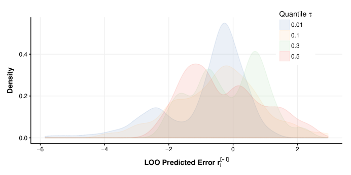
Figure 5: The distributions of LOO residual $r^{[-i]}_{i}$ for flipped cases for various quantiles ($\tau=0.5,\leavevmode\nobreak\ 0.3,\leavevmode\nobreak\ 0.1,\text{ and }0.01$).

4.1.2 Computation for Exact Leave-One-Out CV

We compare two approaches to computing exact LOO CV scores over a set of $N_{\lambda}$ prespecified grid points for the tuning parameter $\lambda$. The first one is based on the proposed $\omega$-path algorithm in Algorithm 1. The other one applies the “$\lambda$-path” algorithm proposed in Li et al. (2007) to the $n$ LOO data sets separately. We make comparisons of the two approaches in terms of theoretical computational complexity as well as practical runtime on simulated data sets.

We first analyze the computational comlexity of applying the “$\lambda$-path” algorithm proposed in Li et al. (2007) $n$ times. Note that the $\lambda$-path algorithm of Li et al. (2007) generates the solution path as $\lambda$ decreases from $\infty$ to $0$. The computation of the exact LOO CV scores involves two components: (i) applying this algorithm to each of the $n$ LOO data sets; and (ii) linearly interpolating the solutions between consecutive grid points. According to Li et al. (2007), the average cost of computing one $\lambda$ path is $O(n^{2}p)$ and the cost for the linear interpolation is $O(N_{\lambda}p)$. Hence, the total cost of computing the exact LOO CV scores in this case is $O(np(n^{2}+N_{\lambda}))$.

For the proposed $\omega$-path aglorithm, it generates each LOO solution directly from the full-data solution. The computation consists of generating $n$ case-weight adjusted $\omega$-paths, whose cost depends on the number of breakpoints for case-weight parameter $\omega$. To simplify the analysis, we work with the average number of $\omega$-breakpoints, denoted by $N_{\omega}$. Our empirical studies show that $N_{\omega}$ is usually small compared to problem dimension (see Table 2). In fact, for extreme values of $\lambda$, we can prove that $N_{\omega}=1$. Therefore, we assume that $N_{\omega}=O(1)$ in our analysis. By inspecting Algorithm 1, the average computational cost at each $\omega$-breakpoint is dominated by Line 15, which computes $b_{0,m}$, $b_{m}$, and $h_{m}$—the slopes of $\beta_{0,\omega}$, $\theta_{\mathcal{E},\omega}$, and $r_{\omega}$. First, the computation of $b_{0,m}$ and $b_{m}$ in (12) and (13) involves inverting a $|\mathcal{E}_{m}|\times|\mathcal{E}_{m}|$ matrix $\tilde{X}_{\mathcal{E}_{m}}\tilde{X}_{\mathcal{E}_{m}}^{\top}$, which typically costs $O(|\mathcal{E}_{m}|^{3})$. This can be reduced further to $O(|\mathcal{E}_{m}|^{2})$ by employing a rank-one updating algorithm (Hager, 1989). Moreover, the cost for computing $h_{m}$ in (15) is $O(np)$. Therefore, the average cost of generating one $\omega$-path at a grid point for $\lambda$ is $O(N_{\omega}(np+|\mathcal{E}_{m}|^{2}))=O(np)$, because $|\mathcal{E}_{m}|\leq\min(n,p+1)$ according to Lemma 3 in Appendix and the assumption that $N_{\omega}=O(1)$. Consequently, the average cost of computing exact LOO CV scores over $N_{\lambda}$ grid points using the proposed $\omega$-path algorithm is $O(N_{\lambda}n^{2}p)$, which is in contrast to the cost of the $\lambda$-path algorithm, $O(np(n^{2}+N_{\lambda}))$. Note that the savings could be large when $N_{\lambda}\ll n$, which is corroborated by an empirical runtime comparison.

Table 2: Average number of $\omega$-breakpoints for various data dimensions and quantiles. The results are averaged over 20 independent simulations with $N_{\lambda}=50$. The 50 grid points for $\lambda\in[0.01,100]$ are equally spaced on the logarithmic scale. The values in the parentheses are the corresponding standard errors.

$\tau$	$n$	$p$	Average number of $\omega$ breakpoints	$n$	$p$	Average number of $\omega$ breakpoints
0.1	100	50	4.409 (0.556)	50	300	0.714 (0.109)
	300	50	4.417 (0.768)	150	300	1.044 (0.192)
0.3	100	50	7.177 (0.686)	50	300	0.714 (0.109)
	300	50	7.724 (1.074)	150	300	1.360 (0.202)
0.5	100	50	7.427 (0.695)	50	300	1.098 (0.119)
	300	50	8.780 (1.119)	150	300	1.635 (0.238)

We present numerical examples comparing the actual runtime performance of the two algorithms. Both algorithms are implemented in C++ with Armadillo package, and were run on a MacBook Pro with Intel Core i5 2.5 GHz CPU and 8 Giga Bytes of main memory. We varied the quantile ($\tau=0.1,\leavevmode\nobreak\ 0.3,\leavevmode\nobreak\ 0.5$), sample size ($n=50$ to 300), number of covariates ($p=50$ to 300), and number of grid points ($N_{\lambda}=20,\leavevmode\nobreak\ 50$). The grid points for $\lambda$ were equally spaced on the logarithmic scale over the range of $\lambda$-breakpoints for the full data fit. For each setting, we had 20 independent replicates and the results are summarized over the replicates. To see the complexity of $\omega$-paths clearly, we recorded the average number of $\omega$-breakpoints when $N_{\lambda}$ is 50 in Table 2.

The runtimes for computation of CV scores depend on the number of grid points and generally a grid for the tuning parameter needs a sufficiently fine resolution to locate the minimum CV score. Figure 6 illustrates that both $N_{\lambda}=20$ and $50$ are adequate for identifying the optimal tuning parameter value for $\lambda$. The solid curves are the complete CV score curves while the dots on the curves correspond to the CV scores at the grid points. The minimizers of the CV scores over the grid points are indicated by the solid vertical lines in the two panels, both of which are close to the dashed vertical lines which correspond to the minimizers of the complete CV score curves.

The runtime comparisons are presented in Figure 7 for $p<n$ settings and Figure 8 for $p>n$ settings. The figures are based on the numerical summaries of the results in Tables 3 and 4 in Appendix. Overall, they show that as the sample size $n$ increases, our proposed $\omega$-path algorithm becomes more scalable than the competing $\lambda$-path algorithm. This is consistent with our earlier analysis of computational complexities.

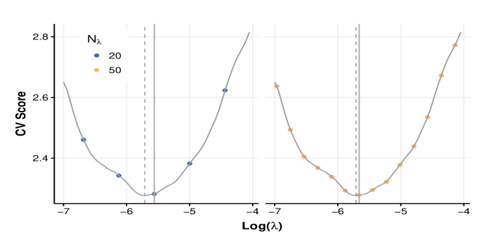
Figure 6: Comparison of two levels of grid resolution in cross validation ($n=100,p=100,\tau=0.5$). The solid curve is a complete CV score curve zoomed in the basin around the optimal $\lambda$, and the dots on the curves are CV scores at the grid points with $N_{\lambda}=20$ in the left panel and $N_{\lambda}=50$ in the right panel.

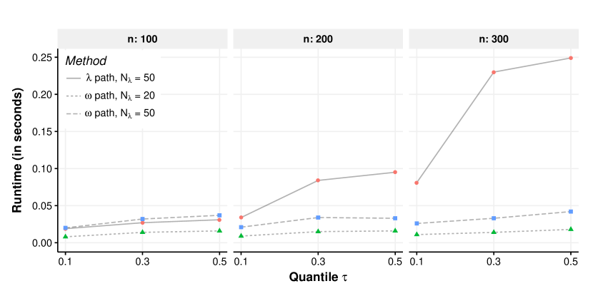
Figure 7: Comparison of the runtime per case (i.e. the total runtime/$n$) between the $\omega$-path and $\lambda$-path algorithms with different data dimensions, quantiles, and levels of grid resolution ($p=50$; $n=100,\leavevmode\nobreak\ 200,\text{ and }300$; $\tau=0.1,\leavevmode\nobreak\ 0.3,\text{ and }0.5$; $N_{\lambda}=20\text{ and }50$).

Figure 8: Comparison of the runtime per case between the $\omega$-path and $\lambda$-path algorithms with different data dimensions, quantiles and levels of grid resolution ($p=300$; $n=50,100\text{ and }150$; $\tau=0.1,\leavevmode\nobreak\ 0.3,\text{ and }0.5$; $N_{\lambda}=20\text{ and }50$).

4.2 Case Influence Graphs

This section presents case influence graphs for ridge regression and $\ell_{2}$-penalized quantile regression with the same data. As is introduced in Section 3.1, case influence graphs show a broad view of the influence of a case on the model as a function of case weight $\omega$. For simplicity, we rescale the generalized Cook’s distance $D_{i^{\star}}(\omega)$ in (18) by replacing the factor $1/p\hat{\sigma}^{2}$ with $1/n$ as

$$\tilde{D}_{i^{\star}}(\omega)=\frac{1}{n}\sum_{i=1}^{n}(\hat{f}(x_{i})-\hat{f}_{\omega}^{i^{\star}}(x_{i}))^{2}.$$ (28)

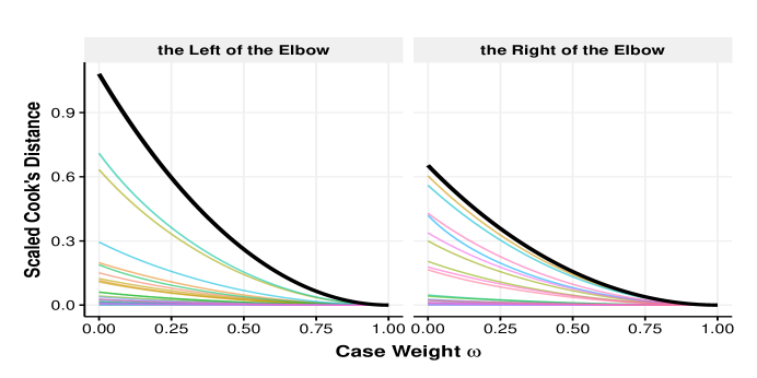
Figure 9: Case influence graphs for ridge regression $(n=50,p=30)$. The influence curves in the left and right panels correspond to cases with negative and positive full-data residuals, respectively. The bold curves correspond to the cases with the most positive or negative full-data residual.

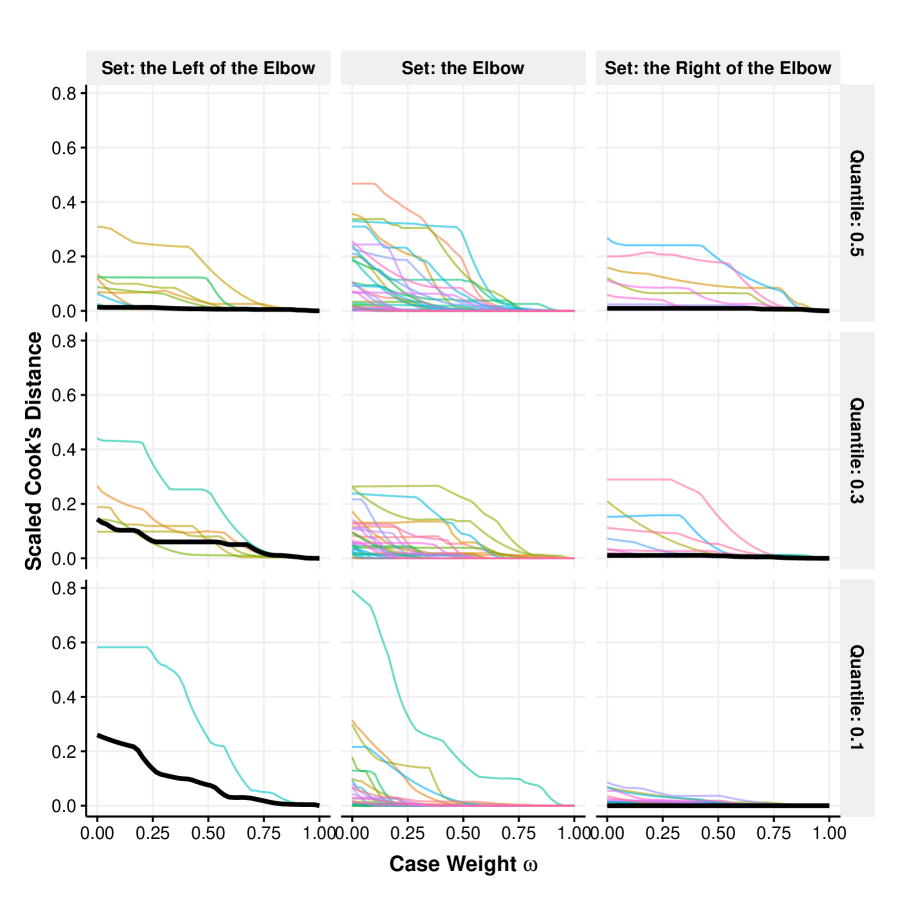
Figure 10: Case influence graphs for penalized quantile regression with various quantiles $(\tau=0.5,\leavevmode\nobreak\ 0.3,\text{ and }0.1)$, $n=50$ and $p=30$. The left, middle and right panels correspond to cases with negative, zero and positive full-data residuals. The bold curves indicate the cases with the most positive or negative full-data residual.

Figure 9 and Figure 10 provide case influence graphs for ridge regression and penalized quantile regression using the same data. Here we remark some major differences in the characteristics of the graphs. As is discussed in Section 3.1, the influence graphs for ridge regression in Figure 9 are smooth, convex and monotonically decreasing in $\omega$, while those for quantile regression in Figure 10 are piecewise quadratic. Moreover, there are few crossings in the curves for ridge regression in Figure 9, suggesting that the standardard Cook’s distance may well be adequate for assessing case influences in ridge regression. By contrast, Figure 10 reveals that for quantile regression, the relation between the case influence graphs and case deletion statistics is more complex and some cases in the elbow set with almost identical standard Cook’s distance can have quite different influence on the model fit.

Additionally, the bold curves marked in Figure 9 and Figure 10 show that for ridge regression, the cases with the most positive or negative full-data residuals have the greatest influence on the model fit, while for quantile regression that is not the case. In fact, for ridge regression, (20) in Proposition 2 implies strong dependence of the case influence on the magnitude of full-data residual. Without much heterogeneity in the case leverages as in our data setting, the cases with the most positive or negative full-data residuals would have the greatest influence. However, for quantile regression, the form of Cook’s generalized distance derived in (3) does not reveal any specific relation between case influence and the magnitude of full-data residual. It is observed that the residuals for the cases with the most positive or negative values tend not to change their signs as $\omega$ decreases from $1$ to $0$, and thus those cases are unlikely to enter the elbow set. They may have little influence on the model fit because the estimated coefficients $(\hat{\beta}_{0,\omega},\hat{\beta}_{\omega})$ only depend on the responses in the elbow set $y_{\mathcal{E}_{m}}$ as shown in Section 2. This is akin to the fact that sample quantiles are not affected by extreme observations. The case influence graphs for quantile regression confirm this expectation, providing another perspective on the robustness of quantile regression.

5 Discussion

In this article, we have proposed a novel path-following algorithm to comptute the leave-one-out cross validation scores exactly for quantile regression with ridge penalty. Numerical analysis has demonstrated that the proposed algorithm compares favorably to an alternative approach in terms of computational efficiency. Theoretically, we have provided a formal proof to establish the validity of the solution path algorithm. Moreover we have demonstrated that our proposed method can be used to efficiently compute the case influence graph, which provides a more comprehensive approach to assessing case influence.

We have primarily focused on $\ell_{2}$ penalized linear quantile regression. Similar case-weight adjusted path following algorithms can be derived for nonparametric quantile regression and $\ell_{1}$ penalized quantile regression. Additionally, following the ideas proposed in Rosset (2009), it may be possible to derive a bi-level solution path for each pair of $(\lambda,\omega)$, or even a tri-level path for each trio of $(\tau,\lambda,\omega)$. Furthermore, the idea of linking the full-data solution and the leave-one-out solution can be extended to classification settings. This will allow us to extend the notion of case influence to classification (Koh and Liang, 2017) and to study the stability of classifiers using case influence measures. How to efficiently assess case influence in classification in itself is an important future direction.

Appendix A Appendix

A.1 Derivation of KKT conditions (6)–(9)

The Lagrangian function associated with (3) is

$$L(\beta_{0},\beta,\xi,\zeta,\alpha,\gamma,\kappa,\rho)=\tau\sum_{i\neq i^{\star}}\xi_{i}+(1-\tau)\sum_{i\neq i^{\star}}\zeta_{i}+\omega\tau\xi_{i^{\star}}+\omega(1-\tau)\zeta_{i^{\star}}+\frac{\lambda}{2}\|\beta\|_{2}^{2}$$

$$\quad+\sum_{i=1}^{n}\alpha_{i}(y_{i}-\beta_{0}-x_{i}^{\top}\beta-\xi_{i})-\sum_{i=1}^{n}\gamma_{i}(y_{i}-\beta_{0}-x_{i}^{\top}\beta+\zeta_{i})-\sum_{i=1}^{n}\kappa_{i}\xi_{i}-\sum_{i=1}^{n}\rho_{i}\zeta_{i}\,,$$

where $\alpha_{i},\gamma_{i},\kappa_{i},\rho_{i}\geq 0$ are the dual variables associated with the inequality constraints, and $\xi_{i}\text{ and }\zeta_{i}\geq 0$ are primal variables introduced in (3). Hence, the Karush-Kuhn-Tucker (KKT) conditions are given by

$$\frac{\partial L}{\partial\beta} = \lambda\beta-\sum_{i=1}^{n}\alpha_{i}x_{i}+\sum_{i=1}^{n}\gamma_{i}x_{i}=0,$$

$$\frac{\partial L}{\partial\beta_{0}} = \sum_{i=1}^{n}(\alpha_{i}-\gamma_{i})=0,$$

$$\frac{\partial L}{\partial\xi_{i}} = -\alpha_{i}-\kappa_{i}+\omega\tau+(1-\omega)\tau\mathbf{1}_{\{i\neq i^{\star}\}}=0,$$

$$\frac{\partial L}{\partial\zeta_{i}} = -\gamma_{i}-\rho_{i}+\omega(1-\tau)+(1-\omega)(1-\tau)\mathbf{1}_{\{i\neq i^{\star}\}}=0,$$

$$\alpha_{i}(y_{i}-\beta_{0}-x_{i}^{\top}\beta-\xi_{i})=0,\quad\gamma_{i}(y_{i}-\beta_{0}-x_{i}^{\top}\beta+\zeta_{i})=0,\quad\kappa_{i}\xi_{i}=0,\quad\rho_{i}\zeta_{i}=0,$$

$$-\zeta_{i}\leq y_{i}-\beta_{0}-x_{i}^{\top}\beta\leq\xi_{i},\quad\alpha_{i}\geq 0,\leavevmode\nobreak\ \gamma_{i}\geq 0,\leavevmode\nobreak\ \kappa_{i}\geq 0,\leavevmode\nobreak\ \rho_{i}\geq 0,\leavevmode\nobreak\ \xi_{i}\geq 0,\leavevmode\nobreak\ \zeta_{i}\geq 0,\leavevmode\nobreak\ i=1,\cdots,n.$$

Defining $\theta_{i}\vcentcolon=\alpha_{i}-\gamma_{i}$ for $i=1,\cdots,n$, we obtain (6) from the first two equations.

Note that when $y_{i}-\beta_{0}-x_{i}^{\top}\beta>0$, we must have $\xi_{i}\geq y_{i}-\beta_{0}-x_{i}^{\top}\beta>0$, which, together with $\kappa_{i}\xi_{i}=0$, implies that $\kappa_{i}=0$. Consequently, we have that $\alpha_{i}=\omega\tau+(1-\omega)\tau\mathbb{I}_{\{i\neq i^{\star}\}}$ and $\xi_{i}=y_{i}-\beta_{0}-x_{i}^{\top}\beta$, because $\alpha_{i}\neq 0$. Moreover, we also have that $\gamma_{i}=0$, because $\gamma_{i}(y_{i}-\beta_{0}-x_{i}^{\top}\beta+\zeta_{i})=0$ and $\zeta_{i}\geq 0$. Hence, $\theta_{i}=\alpha_{i}-\gamma_{i}=\omega\tau+(1-\omega)\tau\mathbb{I}_{\{i\neq i^{\star}\}}$, which proves (9). Similarly, when $y_{i}-\beta_{0}-x_{i}^{\top}\beta<0$, we have that $\gamma_{i}=\omega(1-\tau)+(1-\omega)(1-\tau)\mathbb{I}_{\{i\neq i^{\star}\}}$ and $\alpha_{i}=0$. Hence, $\theta_{i}=\alpha_{i}-\gamma_{i}=-\omega\tau-(1-\omega)\tau\mathbb{I}_{\{i\neq i^{\star}\}}$, which proves (7).

Finally, when $y_{i}-\beta_{0}-x_{i}^{\top}\beta=0$, we must have that $\xi_{i}=0$, because $\alpha_{i}\xi_{i}=0$, $\kappa_{i}\xi_{i}=0$, and $\alpha_{i}+\kappa_{i}=\omega\tau+(1-\omega)\tau\mathbb{I}_{\{i\neq i^{\star}\}}>0$. Similarly, $\zeta_{i}=0$. Moreover, note that $\alpha_{i}\in[0,\omega\tau+(1-\omega)\tau\mathbb{I}_{\{i\neq i^{\star}\}}]$ and $\gamma_{i}\in[0,\omega(1-\tau)+(1-\omega)(1-\tau)\mathbb{I}_{\{i\neq i^{\star}\}}]$. Hence, $\theta_{i}=\alpha_{i}-\gamma_{i}\in[-\omega(1-\tau)-(1-\omega)(1-\tau)\mathbb{I}_{\{i\neq i^{\star}\}}\,,\omega\tau+(1-\omega)\tau\mathbb{I}_{\{i\neq i^{\star}\}}]$, which proves (8).

A.2 Proof of Lemma 3

Lemma 3.

Let $\mathcal{E}_{m}$ be the elbow set defined in Algorithm 1. Suppose that $\{(\tilde{x}_{i},y_{i})\}_{i=1}^{n}$ satisfies the general position condition that any $\min(p+2,n)$ points of $\{(\tilde{x}_{i},y_{i})\}^{n}_{i=1}$ are linearly independent. Then we have $|\mathcal{E}_{m}|\leq p+1$ and $\tilde{X}_{\mathcal{E}_{m}}\tilde{X}_{\mathcal{E}_{m}}^{\top}\succ 0$ for each $m=0,1,\ldots,M$.

Proof.

We prove $\tilde{X}_{\mathcal{E}_{m}}\tilde{X}_{\mathcal{E}_{m}}^{\top}\succ 0$ by showing that (i) $|\mathcal{E}_{m}|\leq p+1$ and (ii) the rows of $\tilde{X}_{\mathcal{E}_{m}}$ are linearly independent.

(i). We prove $|\mathcal{E}_{m}|\leq p+1$ by contradiction. Suppose that $|\mathcal{E}_{m}|\geq p+2$. Then we must have $p+2\leq|\mathcal{E}_{m}|\leq n$. Moreover, by the general position condition, we know that any $\min(n,p+2)=p+2$ points of $\{(\tilde{x}_{i},y_{i})\}^{n}_{i=1}$ are linearly independent, which implies that $rank(\tilde{X}_{\mathcal{E}_{m}},Y_{\mathcal{E}_{m}})\geq p+2$. On the other hand, we can rewrite the KKT condition (8) as

$$y_{\mathcal{E}_{m}}=\beta_{0}{1}_{\mathcal{E}_{m}}+X_{\mathcal{E}_{m}}\beta=\tilde{X}_{\mathcal{E}_{m}}\begin{pmatrix}\beta_{0}\\ \beta\end{pmatrix}\,,$$

which implies that $rank(\tilde{X}_{\mathcal{E}_{m}},Y_{\mathcal{E}_{m}})=rank(\tilde{X}_{\mathcal{E}_{m}})\leq min(p+1,n)\leq p+1$. This is a contradiction. Thus $|\mathcal{E}_{m}|\leq p+1$.

(ii). Since the number of rows of $\tilde{X}_{\mathcal{E}_{m}}$, $|\mathcal{E}_{m}|\leq\min(p+1,n)\leq\min(p+2,n)$ by (i), $rank(\tilde{X}_{\mathcal{E}_{m}},Y_{\mathcal{E}_{m}})=|\mathcal{E}_{m}|$ by the general position condition, which implies that $rank(\tilde{X}_{\mathcal{E}_{m}})=|\mathcal{E}_{m}|$. Thus, the rows of $\tilde{X}_{\mathcal{E}_{m}}$ must be linearly independent. ∎

A.3 Proof of Proposition 1

Since $\lambda r_{\omega}=\lambda(y-\beta_{0,\omega}{\mathbf{1}}-X\beta_{\omega})=\lambda y-\lambda\beta_{0,\omega}{\mathbf{1}}-XX^{\top}\theta_{\omega}$, using the fact that $\lambda\beta_{\omega}=X^{\top}\theta_{\omega}$ from (6), we only need to derive the updating formulas for $\beta_{0,\omega}$ and $\theta_{{\mathcal{E}_{m}},\omega}$.

Let $\tilde{X}=(\mathbf{1},X)$ denote the expanded design matrix with each row $\tilde{x}_{i}^{\top}=(1,x_{i}^{\top})\text{ for }i=1,\cdots,n$. Combining the first two equations in (10), we rewrite (10) as

$$\begin{array}[]{cll}\lambda\begin{pmatrix}0\\ \beta_{\omega}\end{pmatrix}-\tilde{X}^{\top}_{\mathcal{E}_{m}}\theta_{\mathcal{E}_{m},\omega}&=&\tilde{X}^{\top}_{\mathcal{L}_{m}}\theta_{\mathcal{L}_{m},\omega}+\tilde{X}^{\top}_{\mathcal{R}_{m}}\theta_{\mathcal{R}_{m},\omega},\\ \beta_{0,\omega}{1}_{\mathcal{E}_{m}}+\tilde{X}_{\mathcal{E}_{m}}\begin{pmatrix}0\\ \beta_{\omega}\end{pmatrix}&=&y_{\mathcal{E}_{m}}.\end{array}$$ (29)

By eliminating $\beta_{\omega}$ from (29), we have that

$$(\tilde{X}_{\mathcal{E}_{m}}\tilde{X}_{\mathcal{E}_{m}}^{\top})\theta_{\mathcal{E}_{m},\omega}=\big{[}\lambda y_{\mathcal{E}_{m}}-\lambda\beta_{0,\omega}{1}_{\mathcal{E}_{m}}-\tilde{X}_{\mathcal{E}_{m}}\big{(}\tilde{X}^{\top}_{\mathcal{L}_{m}}\theta_{\mathcal{L}_{m},\omega}+\tilde{X}^{\top}_{\mathcal{R}_{m}}\theta_{\mathcal{R}_{m},\omega}\big{)}\big{]}\,,$$ (30)

and

$$1^{\top}_{\mathcal{E}_{m}}\theta_{\mathcal{E}_{m},\omega}=-1^{\top}_{\mathcal{L}_{m}}\theta_{\mathcal{L}_{m},\omega}-1^{\top}_{\mathcal{R}_{m}}\theta_{\mathcal{R}_{m},\omega}.$$ (31)

Under the general position condition, we have that

$$\lambda\beta_{0,\omega}=\frac{1^{\top}_{\mathcal{E}_{m}}(\tilde{X}_{\mathcal{E}_{m}}\tilde{X}_{\mathcal{E}_{m}}^{\top})^{-1}\left(\lambda y_{\mathcal{E}_{m}}-\tilde{X}_{\mathcal{E}_{m}}(\tilde{X}^{\top}_{\mathcal{L}_{m}}\theta_{\mathcal{L}_{m},\omega}+\tilde{X}^{\top}_{\mathcal{R}_{m}}\theta_{\mathcal{R}_{m},\omega})\right)+1^{\top}_{\mathcal{L}_{m}}\theta_{\mathcal{L}_{m},\omega}+1^{\top}_{\mathcal{R}_{m}}\theta_{\mathcal{R}_{m},\omega}}{1^{\top}_{\mathcal{E}_{m}}(\tilde{X}_{\mathcal{E}_{m}}\tilde{X}_{\mathcal{E}_{m}}^{\top})^{-1}1_{\mathcal{E}_{m}}}$$ (32)

and

$$\theta_{\mathcal{E}_{m},\omega}=(\tilde{X}_{\mathcal{E}_{m}}\tilde{X}_{\mathcal{E}_{m}}^{\top})^{-1}\big{[}\lambda y_{\mathcal{E}_{m}}-\lambda\beta_{0,\omega}{1}_{\mathcal{E}_{m}}-\tilde{X}_{\mathcal{E}_{m}}\big{(}\tilde{X}^{\top}_{\mathcal{L}_{m}}\theta_{\mathcal{L}_{m},\omega}+\tilde{X}^{\top}_{\mathcal{R}_{m}}\theta_{\mathcal{R}_{m},\omega}\big{)}\big{]}\,,$$ (33)

where the fact that $\tilde{X}_{\mathcal{E}_{m}}\tilde{X}_{\mathcal{E}_{m}}^{\top}$ is invertible and $1^{\top}_{\mathcal{E}_{m}}(\tilde{X}_{\mathcal{E}_{m}}\tilde{X}_{\mathcal{E}_{m}}^{\top})^{-1}1_{\mathcal{E}_{m}}\neq 0$ are ensured by the general position condition in view of Lemma 3.

From (32) and (33), note that the dependence of $\beta_{0,\omega}$ and $\theta_{\mathcal{E}_{m},\omega}$ on $\omega$ stems from $\theta_{\mathcal{L}_{m},\omega}$ and $\theta_{\mathcal{R}_{m},\omega}$, which may be a function of $\omega$ depending on whether the weighted case $i^{\star}$ is in $\mathcal{L}_{m}\cup\mathcal{R}_{m}$ or not. More specifically, from (7)–(9), if case $i^{\star}\in\mathcal{E}_{m}$, then $\beta_{0,\omega}$ and $\theta_{\mathcal{E}_{m},\omega}$ are independent of $\omega$, because $\theta_{\mathcal{L}_{m},\omega}$ and $\theta_{\mathcal{R}_{m},\omega}$ are both independent of $\omega$. On the other hand, if case $i^{\star}\in\mathcal{L}_{m}\cup\mathcal{R}_{m}$, then $\beta_{0,\omega}$ and $\theta_{\mathcal{E}_{m},\omega}$ are linear in $\omega$ as $\theta_{i^{\star}}=\omega(\tau-\mathbb{I}(i^{\star}\in\mathcal{L}_{m}))$ is linear in $\omega$. As a result, we consider these two cases separately to determine the next breakpoint:

• Case I: $i^{\star}\in\mathcal{L}_{m}\cup\mathcal{R}_{m}$

• Case II: $i^{\star}\in\mathcal{E}_{m}$

I. For Case I, note that

$$\theta_{i^{\star},\omega}=\omega[\tau-\mathbb{I}(i^{\star}\in\mathcal{L}_{m})]\text{ and }\theta_{i,\omega}=[\tau-\mathbb{I}(i\in\mathcal{L}_{m})]\text{ for }i\neq i^{\star}\text{ and }i\in\mathcal{L}_{m}\cup\mathcal{R}_{m}.$$

Hence, taking the difference of (32) at $\omega$ and $\omega_{m}$, and using the fact that only $\theta_{i^{\star},\omega}$ changes with $\omega$, we obtain that

$$\lambda\beta_{0,\omega}-\lambda\beta_{0,\omega_{m}}=b_{0,m}(\omega-\omega_{m})\,,$$ (34)

where

$$b_{0,m}=\frac{1-1_{\mathcal{E}_{m}}^{\top}(\tilde{X}_{\mathcal{E}_{m}}\tilde{X}_{\mathcal{E}_{m}}^{\top})^{-1}\tilde{X}_{\mathcal{E}_{m}}\tilde{x}_{i^{\star}}}{1_{\mathcal{E}_{m}}^{\top}(\tilde{X}_{\mathcal{E}_{m}}\tilde{X}_{\mathcal{E}_{m}}^{\top})^{-1}1_{\mathcal{E}_{m}}}[\tau-\mathbb{I}(i^{\star}\in\mathcal{L}_{m})].$$

Similarly, taking the difference of (33) at $\omega$ and $\omega_{m}$, we obtain that

$$\theta_{\mathcal{E}_{m},\omega}-\theta_{\mathcal{E}_{m},\omega_{m}}$$

$$= -(\tilde{X}_{\mathcal{E}_{m}}\tilde{X}_{\mathcal{E}_{m}}^{\top})^{-1}\left[(\lambda\beta_{0,\omega}-\lambda\beta_{0,\omega_{m}}){1}_{\mathcal{E}_{m}}+\tilde{X}_{\mathcal{E}_{m}}\tilde{x}_{i^{\star}}\{\tau-\mathbb{I}(i^{\star}\in\mathcal{L}_{m})\}(\omega-\omega_{m})\right]$$

$$= -(\tilde{X}_{\mathcal{E}_{m}}\tilde{X}_{\mathcal{E}_{m}}^{\top})^{-1}\left[b_{0,m}1_{\mathcal{E}_{m}}+\tilde{X}_{\mathcal{E}_{m}}\tilde{x}_{i^{\star}}\{\tau-\mathbb{I}(i^{\star}\in\mathcal{L}_{m})\}\right](\omega-\omega_{m})$$

$$= b_{m}(\omega-\omega_{m})\,,$$

where

$$b_{m}=-(\tilde{X}_{\mathcal{E}_{m}}\tilde{X}_{\mathcal{E}_{m}}^{\top})^{-1}\left[b_{0,m}1_{\mathcal{E}_{m}}+\tilde{X}_{\mathcal{E}_{m}}\tilde{x}_{i^{\star}}\{\tau-\mathbb{I}(i^{\star}\in\mathcal{L}_{m})\}\right]\,.$$

This proves (11) and (12). Note that (11) and (12) give how $\theta_{\mathcal{E}_{m},\omega}$ changes as a function of $\omega$. Next, we derive a similar formula for $r_{\omega}$. To that end, multiplying both sides of the first equation in (29) by $\tilde{X}$, we have that for any $\omega\in[\omega_{m+1},\omega_{m}]$,

$$\lambda\tilde{X}\begin{pmatrix}0\\ \beta_{\omega}\end{pmatrix}-\tilde{X}\tilde{X}^{\top}_{\mathcal{E}_{m}}\theta_{\mathcal{E}_{m},\omega}=\tilde{X}\tilde{X}^{\top}_{\mathcal{L}_{m}}\theta_{\mathcal{L}_{m},\omega}+\tilde{X}\tilde{X}^{\top}_{\mathcal{R}_{m}}\theta_{\mathcal{R}_{m},\omega}.$$

Together with (7)–(9), this further implies that

$$\lambda\tilde{X}\begin{pmatrix}0\\ \beta_{\omega}-\beta_{\omega_{m}}\end{pmatrix}=\tilde{X}\tilde{X}^{\top}_{\mathcal{E}_{m}}(\theta_{\mathcal{E}_{m},\omega}-\theta_{\mathcal{E}_{m},\omega_{m}})+\{\tau-\mathbb{I}(i^{\star}\in\mathcal{L}_{m})\}\tilde{X}\tilde{x}_{i^{\star}}(\omega-\omega_{m})\,.$$

Combining this with (34) and (12), we obtain the following result for residual $r_{\omega}$:

$$\lambda r_{\omega}-\lambda r_{\omega_{m}} = \lambda\left(y-\tilde{X}\begin{pmatrix}\beta_{0,\omega}\\ \beta_{\omega}\end{pmatrix}\right)-\lambda\left(y-\tilde{X}\begin{pmatrix}\beta_{0,\omega_{m}}\\ \beta_{\omega_{m}}\end{pmatrix}\right)$$

$$= -\lambda\tilde{X}\begin{pmatrix}0\\ \beta_{\omega}-\beta_{\omega_{m}}\end{pmatrix}-(\lambda\beta_{0,\omega}-\lambda\beta_{0,\omega_{m}})\mathbf{1}$$

$$= -\tilde{X}\tilde{X}^{\top}_{\mathcal{E}_{m}}(\theta_{\mathcal{E}_{m},\omega}-\theta_{\mathcal{E}_{m},\omega_{m}})-\{\tau-\mathbb{I}(i^{\star}\in\mathcal{L}_{m})\}\tilde{X}\tilde{x}_{i^{\star}}(\omega-\omega_{m})-b_{0,m}(\omega-\omega_{m})\mathbf{1}$$

$$= -\tilde{X}\tilde{X}^{\top}_{\mathcal{E}_{m}}b_{m}(\omega-\omega_{m})-\{\tau-\mathbb{I}(i^{\star}\in\mathcal{L}_{m})\}\tilde{X}\tilde{x}_{i^{\star}}(\omega-\omega_{m})-b_{0,m}(\omega-\omega_{m})\mathbf{1}$$

$$= h_{m}(\omega-\omega_{m})\,,$$

where

$$h_{m}=-b_{0,m}\mathbf{1}-\tilde{X}\left[\tilde{X}_{\mathcal{E}_{m}}^{\top}b_{m}+\{\tau-\mathbb{I}(i^{\star}\in\mathcal{L}_{m})\}\tilde{x}_{i^{\star}}\right].$$

This proves (14) and (15).

II. For Case II: $i^{\star}\in\mathcal{E}_{m}$, we will show that $i^{\star}\in\mathcal{E}_{m}$ can only happen when $m=0$, and if that happens, $i^{\star}$ will move from $\mathcal{E}_{0}$ to $\mathcal{L}_{1}\cup\mathcal{R}_{1}$ at the next breakpoint, and stay in $\mathcal{L}_{m}\cup\mathcal{R}_{m}$ for all $m=1,\ldots,M$. We show this by considering two scenarios.

• Scenario 1: if $i^{\star}\in\mathcal{L}_{0}\cup\mathcal{R}_{0}$, then case $i^{\star}$ will stay in $\mathcal{L}_{m}\cup\mathcal{R}_{m}$ for $m=1,\ldots,M$.

• Scenario 2: if $i^{\star}\in\mathcal{E}_{0}$, then $i^{\star}$ will move from $\mathcal{E}_{0}$ to $\mathcal{L}_{1}\cup\mathcal{R}_{1}$ at the next breakpoint, and stay in $\mathcal{L}_{m}\cup\mathcal{R}_{m}$ for $m=1,\ldots,M$.

For Scenario 1, we show that if $i^{\star}\in\mathcal{L}_{m}\cup\mathcal{R}_{m}$, then case $i^{\star}$ will not move from $\mathcal{L}_{m}\cup\mathcal{R}_{m}$ to $\mathcal{E}_{m}$ at the next breakpoint. We prove this by showing that the slope of the residual for case $i^{\star}$ over $(\omega_{m+1},\omega_{m})$ is negative if $i^{\star}\in\mathcal{R}_{m}$; and positive if $i^{\star}\in\mathcal{L}_{m}$. Suppose that $i^{\star}\in\mathcal{R}_{m}$. In view of (14) and (15), we need to show that $\frac{\partial r_{i^{\star},\omega}}{\partial\omega}=h_{i^{\star},m}<0$, or equivalently,

$$h_{i^{\star},m}=-b_{0,m}-\tilde{x}_{i^{\star}}^{\top}\left[\tilde{X}_{\mathcal{E}_{m}}^{\top}b_{m}+\tilde{x}_{i^{\star}}\tau\right]<0\,.$$ (35)

By (12) and (13), we can show that

$$h_{i^{\star},m} = -\left(b_{0,m}+\tilde{x}_{i^{\star}}^{\top}\left[\tilde{X}_{\mathcal{E}_{m}}^{\top}b_{m}+\tilde{x}_{i^{\star}}\tau\right]\right)$$

$$= -\left(b_{0,m}-\tilde{x}_{i^{\star}}^{\top}\left[\tilde{X}_{\mathcal{E}_{m}}^{\top}\left((\tilde{X}_{\mathcal{E}_{m}}\tilde{X}_{\mathcal{E}_{m}}^{\top})^{-1}\left[b_{0,m}1_{\mathcal{E}_{m}}+\tilde{X}_{\mathcal{E}_{m}}\tilde{x}_{i^{\star}}\{\tau-\mathbb{I}(i^{\star}\in\mathcal{L}_{m})\}\right]\right)+\tilde{x}_{i^{\star}}\tau\right]\right)$$

$$= -\left(b_{0,m}-\tilde{x}_{i^{\star}}^{\top}\tilde{X}^{\top}_{\mathcal{E}_{m}}(\tilde{X}_{\mathcal{E}_{m}}\tilde{X}_{\mathcal{E}_{m}}^{\top})^{-1}b_{0,m}{1}_{\mathcal{E}_{m}}-\tilde{x}_{i^{\star}}^{\top}\tilde{X}^{\top}_{\mathcal{E}_{m}}(\tilde{X}_{\mathcal{E}_{m}}\tilde{X}_{\mathcal{E}_{m}}^{\top})^{-1}\tilde{X}_{\mathcal{E}_{m}}\tilde{x}_{i^{\star}}\tau+\tilde{x}_{i^{\star}}^{\top}\tilde{x}_{i^{\star}}\tau\right)$$

$$= -b_{0,m}\left(1-\tilde{x}_{i^{\star}}^{\top}\tilde{X}^{\top}_{\mathcal{E}_{m}}(\tilde{X}_{\mathcal{E}_{m}}\tilde{X}_{\mathcal{E}_{m}}^{\top})^{-1}{1}_{\mathcal{E}_{m}}\right)-\tau\tilde{x}_{i^{\star}}^{\top}\big{(}I-\tilde{X}_{\mathcal{E}_{m}}^{\top}(\tilde{X}_{\mathcal{E}_{m}}\tilde{X}_{\mathcal{E}_{m}}^{\top})^{-1}\tilde{X}_{\mathcal{E}_{m}}\big{)}\tilde{x}_{i^{\star}}$$

$$= -\tau\frac{(1-1^{\top}_{\mathcal{E}_{m}}(\tilde{X}_{\mathcal{E}_{m}}\tilde{X}_{\mathcal{E}_{m}}^{\top})^{-1}\tilde{X}_{\mathcal{E}_{m}}\tilde{x}_{i^{\star}})^{2}}{1^{\top}_{\mathcal{E}_{m}}(\tilde{X}_{\mathcal{E}_{m}}\tilde{X}_{\mathcal{E}_{m}}^{\top})^{-1}1_{\mathcal{E}_{m}}}-\tau\tilde{x}_{i^{\star}}^{\top}\big{(}I-\tilde{X}_{\mathcal{E}_{m}}^{\top}(\tilde{X}_{\mathcal{E}_{m}}\tilde{X}_{\mathcal{E}_{m}}^{\top})^{-1}\tilde{X}_{\mathcal{E}_{m}}\big{)}\tilde{x}_{i^{\star}}<0\,,$$

where the last inequality uses the fact that $\tilde{x}_{i^{\star}}^{\top}\big{(}I-\tilde{X}_{\mathcal{E}_{m}}^{\top}(\tilde{X}_{\mathcal{E}_{m}}\tilde{X}_{\mathcal{E}_{m}}^{\top})^{-1}\tilde{X}_{\mathcal{E}_{m}}\big{)}\tilde{x}_{i^{\star}}>0$ under the general position condition, which can be shown as follows. Note that the rows of $\tilde{X}_{\mathcal{E}_{m}}$ and $\tilde{x}_{i}$ are linearly independent since $|\mathcal{E}_{m}\cup\{i\}|=|\mathcal{E}_{m-1}|\leq\min(n,p+1)\leq\min(n,p+2)$. Hence, $\tilde{x}_{i}^{\top}\big{(}I-\tilde{X}^{\top}_{\mathcal{E}_{m}}\big{(}\tilde{X}_{\mathcal{E}_{m}}\tilde{X}_{\mathcal{E}_{m}}^{\top}\big{)}^{-1}\tilde{X}_{\mathcal{E}_{m}}\big{)}\tilde{x}_{i}>0$ since $\tilde{X}^{\top}_{\mathcal{E}_{m}}\big{(}\tilde{X}_{\mathcal{E}_{m}}\tilde{X}_{\mathcal{E}_{m}}^{\top}\big{)}^{-1}\tilde{X}_{\mathcal{E}_{m}}$ is the projection matrix for the row space of $\tilde{X}_{\mathcal{E}_{m}}$ and $\tilde{X}^{\top}_{\mathcal{E}_{m}}\big{(}\tilde{X}_{\mathcal{E}_{m}}\tilde{X}_{\mathcal{E}_{m}}^{\top}\big{)}^{-1}\tilde{X}_{\mathcal{E}_{m}}\tilde{x}_{i}\neq\tilde{x}_{i}$.

Similarly we can also show that when $i^{\star}\in\mathcal{L}_{m}$,

$$h_{i^{\star},m} = (1-\tau)\frac{(1-1^{\top}_{\mathcal{E}_{m}}(\tilde{X}_{\mathcal{E}_{m}}\tilde{X}_{\mathcal{E}_{m}}^{\top})^{-1}\tilde{X}_{\mathcal{E}_{m}}\tilde{x}_{i^{\star}})^{2}}{1^{\top}_{\mathcal{E}_{m}}(\tilde{X}_{\mathcal{E}_{m}}\tilde{X}_{\mathcal{E}_{m}}^{\top})^{-1}1_{\mathcal{E}_{m}}}+(1-\tau)\tilde{x}_{i^{\star}}^{\top}\big{(}I-\tilde{X}_{\mathcal{E}_{m}}^{\top}(\tilde{X}_{\mathcal{E}_{m}}\tilde{X}_{\mathcal{E}_{m}}^{\top})^{-1}\tilde{X}_{\mathcal{E}_{m}}\big{)}\tilde{x}_{i^{\star}}$$ (36)

$$> 0\,.$$

This finishes the proof for Scenario 1.

For Scenario 2, note that when $i^{\star}\in\mathcal{E}_{0}$, all the residuals and $\theta_{\omega}$ are constant as $\theta_{\omega}$ and $(\beta_{0,\omega},\beta_{\omega})$ are independent of $\omega$ for $\omega\in[\omega_{1},1]$. As a result, the next breakpoint $\omega_{1}$ can be determined by setting $\theta_{i^{\star},\omega_{0}}=\omega\tau\text{ or }\omega(\tau-1)$, that is,

$$\omega_{1}=\begin{cases}\frac{{\theta}_{i^{\star},\omega_{0}}}{\tau}&\text{ if }0<{\theta}_{i^{\star},\omega_{0}}<\tau\\ \frac{{\theta}_{i^{\star},\omega_{0}}}{\tau-1}&\text{ if }\tau-1<{\theta}_{i^{\star},\omega_{0}}<0\\ 0&\text{ if }{\theta}_{i^{\star},\omega_{0}}=0\end{cases},\,\text{ or }\,\omega_{1}=\frac{{\theta}_{i^{\star},\omega_{0}}}{\tau-\mathbb{I}({\theta}_{i^{\star},\omega_{0}}<0)}\,,$$ (37)

and $i^{\star}$ will move from $\mathcal{E}_{0}$ to $\mathcal{L}_{1}$ or $\mathcal{R}_{1}$ at $\omega_{1}$. After $\omega_{1}$, by the same argument used for Scenario 1, we can show that $i^{\star}$ will stay in $\mathcal{L}_{m}\cup\mathcal{R}_{m}$ for $m=1,\ldots,M$. This proves Scenario 2.

In summary, $i^{\star}\in\mathcal{E}_{m}$ can only happen when $m=0$, and if that happens, $i^{\star}$ will move from $\mathcal{E}_{0}$ to $\mathcal{L}_{1}$ or $\mathcal{R}_{1}$ at the next breakpoint, and stay in $\mathcal{L}_{m}\cup\mathcal{R}_{m}$ for $m=1,\ldots,M$. This completes the proof of Proposition 1.

A.4 Proof of Theorem 1

We only need to show that the case-weight adjusted path $(\hat{\beta}_{0,\omega},\hat{\beta}_{\omega},\hat{\theta}_{\omega})$ generated by Algorithm 1 satisfies all the KKT conditions in (6)–(9). Our plan is to show that: (i) the initial full-data solution $(\hat{\beta}_{0,\omega_{0}},\hat{\beta}_{\omega_{0}})$ together with $\hat{\theta}_{\omega_{0}}$ specified in Line 3 satisfies the KKT conditions at $\omega=\omega_{0}$; (ii) if $i^{\star}\in\mathcal{E}_{0}$, then for each $\omega\in[\omega_{1},1]$, $(\hat{\beta}_{0,\omega},\hat{\beta}_{\omega},\hat{\theta}_{\omega})$ in Line 7 satisfies the KKT conditions; and (iii) after Line 13 in Algorithm 1, $i^{\star}\notin\mathcal{E}_{m}$ for each $m$, and $(\hat{\beta}_{0,\omega},\hat{\beta}_{\omega},\hat{\theta}_{\omega})$ in Line 17 satisfies the KKT conditions.

(i) Note that $(\hat{\beta}_{0,\omega_{0}},\hat{\beta}_{\omega_{0}})$ is the full-data solution. Thus, there must exist a vector $\theta\in\mathbb{R}^{n}$ such that $(\hat{\beta}_{0,\omega_{0}},\hat{\beta}_{\omega_{0}},\theta)$ satisfies the KKT conditions of (6)–(9). On the other hand, similar to the derivation of (33), we can show that $\theta$ must be unique and equal to $\hat{\theta}_{\omega_{0}}$ specified in Algorithm 1 given $(\hat{\beta}_{0,\omega_{0}},\hat{\beta}_{\omega_{0}})$. Hence, $(\hat{\beta}_{0,\omega_{0}},\hat{\beta}_{\omega_{0}},\hat{\theta}_{\omega_{0}})$ satisfies the KKT conditions.

(ii) If the weighted case $i^{\star}\in\mathcal{E}_{0}$, then for each $\omega\in[\omega_{1},1]$, $(\hat{\beta}_{0,\omega},\hat{\beta}_{\omega},\hat{\theta}_{\omega})=(\hat{\beta}_{0,\omega_{0}},\hat{\beta}_{\omega_{0}},\hat{\theta}_{\omega_{0}})$, and thus it must also satisfy the KKT conditions (6)–(9), because the only condition in (6)–(9) that involves $\omega$ is $\theta_{i^{\star},\omega_{0}}\in[\omega(\tau-1),\omega\tau]$, which remains to be true when $\omega\geq\omega_{1}=\frac{\hat{\theta}_{i^{\star},\omega_{0}}}{\tau-\mathbb{I}(\hat{\theta}_{i^{\star},\omega_{0}}<0)}$.

(iii) We use induction on $m$ to show that $(\hat{\beta}_{0,\omega},\hat{\beta}_{\omega},\hat{\theta}_{\omega})$ satisfies the KKT conditions for $\omega\in[\omega_{m+1},\omega_{m}]$ and $i^{\star}\notin\mathcal{E}_{m}$, after Line 13 of Algorithm 1. First we show that $i^{\star}\notin\mathcal{E}_{m}$ after Line 13 of Algorithm 1. Using similar arguments in Part II of the proof of Proposition 1, we can show that if $i^{\star}\in\mathcal{L}_{m}\cup\mathcal{R}_{m}$, then case $i^{\star}$ will not move from $\mathcal{L}_{m}\cup\mathcal{R}_{m}$ to $\mathcal{E}_{m}$ at the next breakpoint. This can be verified using (35) and (36), both of which are still valid here since $b_{0,m}$ and $b_{m}$ in Line 15 are computed according to (12) and (13) in Proposition 1. Hence, we must have $i^{\star}\in\mathcal{L}_{m}\cup\mathcal{R}_{m}$ after Line 13 of Algorithm 1.

Next, we show that $(\hat{\beta}_{0,\omega},\hat{\beta}_{\omega},\hat{\theta}_{\omega})$ satisfies the KKT conditions for $\omega\in[\omega_{m+1},\omega_{m}]$ after Line 13 of Algorithm 1, provided that $i^{\star}\notin\mathcal{E}_{m}$. In other words, we show that for each $\omega\in[\omega_{m+1},\omega_{m}]$, $(\hat{\beta}_{0,\omega},\hat{\beta}_{\omega},\hat{\theta}_{\omega})$ generated by Algorithm 1 satisfies the KKT conditions provided that $(\hat{\beta}_{0,\omega_{m}},\hat{\beta}_{\omega_{m}},\hat{\theta}_{\omega_{m}})$ satisfies the KKT conditions at breakpoint $\omega_{m}$. Note that the KKT conditions consist of equality conditions and inequality conditions. We verify them separately.

Equality conditions: First, we verify that the following equality conditions are satisfied between breakpoints $\omega_{m}$ and $\omega_{m+1}$:

$$\begin{array}[]{ll}\hat{\theta}_{\mathcal{L}_{m}\setminus\{i^{\star}\},\omega}=(\tau-1){1}_{\mathcal{L}_{m}\setminus\{i^{\star}\}},\quad\hat{\theta}_{\mathcal{R}_{m}\setminus\{i^{\star}\},\omega}=\tau{1}_{\mathcal{R}_{m}\setminus\{i^{\star}\}},\quad\hat{\theta}_{i^{\star},\omega}=\omega(\tau-\mathbb{I}(i^{\star}\in\mathcal{L}_{m}))\\ \tilde{X}^{\top}\hat{\theta}_{\omega}=\begin{pmatrix}0\\ \lambda\hat{\beta}_{\omega}\end{pmatrix},\quad\tilde{X}_{\mathcal{E}_{m}}\begin{pmatrix}\hat{\beta}_{0,m}\\ \hat{\beta}_{m}\end{pmatrix}=y_{\mathcal{E}_{m}}.\end{array}$$ (38)

Since the above equality conditions are satisfied at $\omega=\omega_{m}$, it is sufficient to show that for each $\omega\in[\omega_{m+1},\omega_{m}]$,

$$\tilde{X}^{\top}(\hat{\theta}_{\omega}-\hat{\theta}_{\omega_{m}})=\begin{pmatrix}0\\ \lambda(\hat{\beta}_{\omega}-\hat{\beta}_{\omega_{m}})\end{pmatrix}$$ (39a)

$$\tilde{X}_{\mathcal{E}_{m}}\begin{pmatrix}\hat{\beta}_{0,\omega}-\hat{\beta}_{0,\omega_{m}}\\ \hat{\beta}_{\omega}-\hat{\beta}_{\omega_{m}}\end{pmatrix}=\mathbf{0}.$$ (39b)

To prove (39a), first we see that

$$\tilde{X}^{\top}(\hat{\theta}_{\omega}-\hat{\theta}_{\omega_{m}}) =\tilde{X}_{\mathcal{L}_{m}}^{\top}(\hat{\theta}_{\mathcal{L}_{m},\omega}-\hat{\theta}_{\mathcal{L}_{m},\omega_{m}})+\tilde{X}_{\mathcal{R}_{m}}^{\top}(\hat{\theta}_{\mathcal{R}_{m},\omega}-\hat{\theta}_{\mathcal{R}_{m},\omega_{m}})+\tilde{X}_{\mathcal{E}_{m}}^{\top}(\hat{\theta}_{\mathcal{E}_{m},\omega}-\hat{\theta}_{\mathcal{E}_{m},\omega_{m}})$$

$$=\{\tau-\mathbb{I}(i^{\star}\in\mathcal{L}_{m})\}\tilde{x}_{i^{\star}}(\omega-\omega_{m})+\tilde{X}^{\top}_{\mathcal{E}_{m}}b_{m}(\omega-\omega_{m})\quad\quad\mbox{by \eqref{eq:theta_slopes}}$$

$$=\left(\{\tau-\mathbb{I}(i^{\star}\in\mathcal{L}_{m})\}\tilde{x}_{i^{\star}}+\tilde{X}^{\top}_{\mathcal{E}_{m}}b_{m}\right)(\omega-\omega_{m})$$

$$=\begin{pmatrix}\left(\{\tau-\mathbb{I}(i^{\star}\in\mathcal{L}_{m})\}+1_{\mathcal{E}_{m}}^{\top}b_{m}\right)(\omega-\omega_{m})\\ \left(\{\tau-\mathbb{I}(i^{\star}\in\mathcal{L}_{m})\}x_{i^{\star}}+X_{\mathcal{E}_{m}}^{\top}b_{m}\right)(\omega-\omega_{m})\end{pmatrix}\,.$$

Moreover, by (12) and (13), we can show that

$$-1_{\mathcal{E}_{m}}^{\top}b_{m} =1_{\mathcal{E}_{m}}^{\top}(\tilde{X}_{\mathcal{E}_{m}}\tilde{X}_{\mathcal{E}_{m}}^{\top})^{-1}\left[b_{0,m}1_{\mathcal{E}_{m}}+\tilde{X}_{\mathcal{E}_{m}}\tilde{x}_{i^{\star}}\{\tau-\mathbb{I}(i^{\star}\in\mathcal{L}_{m})\}\right]$$

$$=b_{0,m}1_{\mathcal{E}_{m}}^{\top}(\tilde{X}_{\mathcal{E}_{m}}\tilde{X}_{\mathcal{E}_{m}}^{\top})^{-1}1_{\mathcal{E}_{m}}+1_{\mathcal{E}_{m}}^{\top}(\tilde{X}_{\mathcal{E}_{m}}\tilde{X}_{\mathcal{E}_{m}}^{\top})^{-1}\tilde{X}_{\mathcal{E}_{m}}\tilde{x}_{i^{\star}}\{\tau-\mathbb{I}(i^{\star}\in\mathcal{L}_{m})\}$$

$$=\left(1-1_{\mathcal{E}_{m}}^{\top}(\tilde{X}_{\mathcal{E}_{m}}\tilde{X}_{\mathcal{E}_{m}}^{\top})^{-1}\tilde{X}_{\mathcal{E}_{m}}\tilde{x}_{i^{\star}}\right)\{\tau-\mathbb{I}(i^{\star}\in\mathcal{L}_{m})\}+\ 1_{\mathcal{E}_{m}}^{\top}(\tilde{X}_{\mathcal{E}_{m}}\tilde{X}_{\mathcal{E}_{m}}^{\top})^{-1}\tilde{X}_{\mathcal{E}_{m}}\tilde{x}_{i^{\star}})\{\tau-\mathbb{I}(i^{\star}\in\mathcal{L}_{m})\}$$

$$=\tau-\mathbb{I}(i^{\star}\in\mathcal{L}_{m}).$$

Combining this with Line 17 of Algorithm 1, we obtain (39a).

To prove (39b), by (39a), (34), (11), and (12), it follows that

$$\lambda\tilde{X}_{\mathcal{E}_{m}}\begin{pmatrix}\hat{\beta}_{0,\omega}-\hat{\beta}_{0,\omega_{m}}\\ \hat{\beta}_{\omega}-\hat{\beta}_{\omega_{m}}\end{pmatrix} =\tilde{X}_{\mathcal{E}_{m}}\begin{pmatrix}\lambda(\hat{\beta}_{0,\omega}-\hat{\beta}_{0,\omega_{m}})\\ \mathbf{0}\end{pmatrix}+\tilde{X}_{\mathcal{E}_{m}}\begin{pmatrix}0\\ \lambda(\hat{\beta}_{\omega}-\hat{\beta}_{\omega_{m}})\end{pmatrix}$$

$$=\lambda(\hat{\beta}_{0,\omega}-\hat{\beta}_{0,\omega_{m}}){1}_{\mathcal{E}_{m}}+\tilde{X}_{\mathcal{E}_{m}}\tilde{X}^{\top}(\hat{\theta}_{\omega}-\hat{\theta}_{\omega_{m}})$$

$$=\left(b_{0,m}{1}_{\mathcal{E}_{m}}+\tilde{X}_{\mathcal{E}_{m}}\tilde{X}_{\mathcal{E}_{m}}^{\top}b_{m}+\tilde{X}_{\mathcal{E}_{m}}\tilde{x}_{i^{\star}}\{\tau-\mathbb{I}(i^{\star}\in\mathcal{L}_{m})\}\right)(\omega-\omega_{m})$$

$$=\biggl{(}b_{0,m}{1}_{\mathcal{E}_{m}}+\tilde{X}_{\mathcal{E}_{m}}\tilde{x}_{i^{\star}}\{\tau-\mathbb{I}(i^{\star}\in\mathcal{L}_{m})\}-$$

$$\phantom{{}=1}\tilde{X}_{\mathcal{E}_{m}}\tilde{X}_{\mathcal{E}_{m}}^{\top}(\tilde{X}_{\mathcal{E}_{m}}\tilde{X}_{\mathcal{E}_{m}}^{\top})^{-1}\left[b_{0,m}{1}_{\mathcal{E}_{m}}+\tilde{X}_{\mathcal{E}_{m}}\tilde{x}_{i^{\star}}\{\tau-\mathbb{I}(i^{\star}\in\mathcal{L}_{m})\}\right]\biggr{)}(\omega-\omega_{m})$$

$$=0.$$

Inequality conditions: Next we verify the inequality conditions between breakpoints $\omega_{m}$ and $\omega_{m+1}$. For this, we consider two cases: $m=\mathbb{I}(i^{\star}\in\mathcal{E}_{0})$ and $m\geq\mathbb{I}(i^{\star}\in\mathcal{E}_{0})+1$. In the first case, if $i^{\star}\notin\mathcal{E}_{0}$, then $m=0$, and all inequality conditions are trivially satisfied for $\omega\in[\omega_{1},1]$. If $i^{\star}\in\mathcal{E}_{0}$, then $m=1$. Now for $\omega\in[\omega_{2},\omega_{1}]$, we need to verify that $r_{i^{\star},\omega}>0$ if $i^{\star}\in\mathcal{R}_{1}$, and $r_{i^{\star},\omega}<0$ if $i^{\star}\in\mathcal{L}_{1}$. In fact, by similar arguments used in the proof of Part II of Proposition 1, it can be shown that the residual of case $i^{\star}$ will increase if $i^{\star}\in\mathcal{R}_{1}$ and will decrease if $i^{\star}\in\mathcal{L}_{1}$. Moreover, since $i^{\star}\in\mathcal{E}_{0}$, we must have $r_{i^{\star},\omega_{1}}=0$. Combining, we have that that $r_{i^{\star},\omega}>0$ if $i^{\star}\in\mathcal{R}_{1}$ and $r_{i^{\star},\omega}<0$ if $i^{\star}\in\mathcal{L}_{1}$.

In the second case of $m\geq\mathbb{I}(i^{\star}\in\mathcal{E}_{0})+1$, we have that $i^{\star}\notin\mathcal{E}_{m}$ and $i^{\star}\notin\mathcal{E}_{m-1}$ since $i^{\star}\notin\mathcal{E}_{m}$ after Line 13. In addition, as we have shown before, the sign of the residual of case $i^{\star}$ does not change after Line 13. Under these conditions, we next show that all the inequality conditions are satisfied by verifying that the three rules in Algorithm 1 to update the elbow set and non-elbow sets at each breakpoint are consistent with the signs of resulting residuals. Specifically, we need to verify that, for rule (a), if $\hat{\theta}_{i,\omega_{m}}=\tau$ for some $i\in\mathcal{E}_{m-1}$, then $r_{i,\omega}>0$ for $\omega\in(\omega_{m+1},\omega_{m})$; for rule (b), if $\hat{\theta}_{i,\omega_{m}}=\tau-1$ for some $i\in\mathcal{E}_{m-1}$, then $r_{i,\omega}<0$ for $\omega\in(\omega_{m+1},\omega_{m})$, and for rule (c), if $r_{i,\omega_{m}}=0$ for some $i\in\mathcal{L}_{m-1}\cup\mathcal{R}_{m-1}$, then $\theta_{i,\omega}\in(\tau-1,\tau)$ for $\omega\in(\omega_{m+1},\omega_{m})$.

For rule (a), if there exists $i\in\mathcal{E}_{m-1}$ such that $\hat{\theta}_{i,\omega_{m}}=\tau$ at $\omega_{m}$, the rule sets $\mathcal{E}_{m}=\mathcal{E}_{m-1}\setminus\{i\}$ and $\mathcal{R}_{m}=\mathcal{R}_{m-1}\cup\{i\}$. We need to show that $r_{i,\omega}>0$ for $\omega\in(\omega_{m+1},\omega_{m})$. Since $r_{i,\omega_{m}}=0$, we need to show that $h_{i,m}$—the slope of $r_{i,\omega}$—is negative. In view of (15) and the fact that $\mathcal{E}_{m}=\mathcal{E}_{m-1}\setminus\{i\}$, we need to prove that

$$-h_{i,m}=b_{0,m}+\tilde{x}_{i}^{\top}[\tilde{X}^{\top}_{\mathcal{E}_{m-1}\setminus\{i\}}b_{m}+\tilde{x}_{i^{\star}}(\tau-\mathbb{I}(i^{\star}\in\mathcal{L}_{m})]>0.$$ (40)

Since $i\in\mathcal{E}_{m-1}$, we have that $\lambda r_{i,\omega}\equiv 0$ for $\omega\in(\omega_{m},\omega_{m-1}]$, which implies that its slope $h_{i,m-1}=0$. This, together with (15), implies that

$$-h_{i,m-1} = b_{0,m-1}+\tilde{x}_{i}^{\top}[\tilde{X}^{\top}_{\mathcal{E}_{m-1}}b_{m-1}+\tilde{x}_{i^{\star}}(\tau-\mathbb{I}(i^{\star}\in\mathcal{L}_{m-1}))]$$ (41)

$$= b_{0,m-1}+\tilde{x}_{i}^{\top}[\tilde{X}^{\top}_{\mathcal{E}_{m}}b_{\mathcal{E}_{m},m-1}+\tilde{x}_{i}b_{i,m-1}+\tilde{x}_{i^{\star}}(\tau-\mathbb{I}(i^{\star}\in\mathcal{L}_{m-1}))]=0\,.$$

Moreover, note that $\mathbb{I}(i^{\star}\in\mathcal{L}_{m-1})=\mathbb{I}(i^{\star}\in\mathcal{L}_{m})$ for $m\geq 1+\mathbb{I}(i^{\star}\in\mathcal{E}_{0})$ since $i^{\star}\notin\mathcal{E}_{m}$ and $i\neq i^{\star}$. In view of (41), (40) is equivalent to

$$b_{0,m}+\tilde{x}_{i}^{\top}\tilde{X}^{\top}_{\mathcal{E}_{m-1}\setminus\{i\}}b_{m}>b_{0,m-1}+\tilde{x}_{i}^{\top}\tilde{X}^{\top}_{\mathcal{E}_{m-1}\setminus\{i\}}b_{\mathcal{E}_{m-1}\setminus\{i\},m-1}+\tilde{x}_{i}^{\top}\tilde{x}_{i}b_{i,m-1}\,,$$

or

$$(b_{0,m}-b_{0,m-1})+\tilde{x}_{i}^{\top}\tilde{X}^{\top}_{\mathcal{E}_{m}}(b_{m}-b_{\mathcal{E}_{m},m-1})-\tilde{x}_{i}^{\top}\tilde{x}_{i}b_{i,m-1}>0.$$ (42)

Next we plan to show that

$$(b_{m}-b_{\mathcal{E}_{m},m-1})-\tilde{x}_{i}^{\top}\tilde{x}_{i}b_{i,m-1}$$ (43)

$$= b_{i,m-1}\left(-\frac{\big{(}{1_{\mathcal{E}_{m}}}^{\top}\big{(}\tilde{X}_{\mathcal{E}_{m}}\tilde{X}_{\mathcal{E}_{m}}^{\top}\big{)}^{-1}\tilde{X}_{\mathcal{E}_{m}}\tilde{x}_{i}-1\big{)}^{2}}{{1_{\mathcal{E}_{m}}}^{\top}\big{(}\tilde{X}_{\mathcal{E}_{m}}\tilde{X}_{\mathcal{E}_{m}}^{\top}\big{)}^{-1}{1_{\mathcal{E}_{m}}}}-\tilde{x}_{i}^{\top}\big{(}I-\tilde{X}^{\top}_{\mathcal{E}_{m}}\big{(}\tilde{X}_{\mathcal{E}_{m}}\tilde{X}_{\mathcal{E}_{m}}^{\top}\big{)}^{-1}\tilde{X}_{\mathcal{E}_{m}}\big{)}\tilde{x}_{i}\right).$$

To that end, from the second equation in (38), we know that $1^{\top}\hat{\theta}_{\omega}=0$ for $\omega\in(\omega_{m+1},\omega_{m}]$. Hence, for any $\omega\in(\omega_{m+1},\omega_{m})$,

$$\begin{array}[]{ll}1_{\mathcal{E}_{m}}^{\top}\hat{\theta}_{\mathcal{E}_{m},\omega}+1_{\mathcal{L}_{m}}^{\top}\hat{\theta}_{\mathcal{L}_{m},\omega}+1_{\mathcal{R}_{m}}^{\top}\hat{\theta}_{\mathcal{R}_{m},\omega}=0\\ 1_{\mathcal{E}_{m}}^{\top}\hat{\theta}_{\mathcal{E}_{m},\omega_{m}}+1_{\mathcal{L}_{m}}^{\top}\hat{\theta}_{\mathcal{L}_{m},\omega_{m}}+1_{\mathcal{R}_{m}}^{\top}\hat{\theta}_{\mathcal{R}_{m},\omega_{m}}=0\end{array}\,.$$ (44)

Taking difference of the above two equations and using the updating formula for $\hat{\theta}_{\mathcal{E}_{m},\omega}$, we obtain that

$$1_{\mathcal{E}_{m}}^{\top}b_{m}(\omega-\omega_{m})+(\tau-\mathbb{I}(i^{\star}\in\mathcal{L}_{m}))(\omega-\omega_{m})=0.$$ (45)

Dividing both sides by $\omega-\omega_{m}$, (45) reduces to

$$1_{\mathcal{E}_{m}}^{\top}b_{m}+(\tau-\mathbb{I}(i^{\star}\in\mathcal{L}_{m}))=0.$$

Similarly, we also have that

$$1_{\mathcal{E}_{m-1}}^{\top}b_{m-1}+(\tau-\mathbb{I}(i^{\star}\in\mathcal{L}_{m-1}))=0\,.$$

Taking the difference and using the fact that $\mathbb{I}(i^{\star}\in\mathcal{L}_{m-1})=\mathbb{I}(i^{\star}\in\mathcal{L}_{m})$ for $m\geq 1+\mathbb{I}(i^{\star}\in\mathcal{E}_{0})$, we obtain that

$$b_{i,m-1}=1_{\mathcal{E}_{m}}^{\top}b_{m}-1_{\mathcal{E}_{m}}^{\top}b_{\mathcal{E}_{m},m-1}:=1_{\mathcal{E}_{m}}^{\top}\Delta_{\mathcal{E}_{m}},$$ (46)

where $\Delta_{\mathcal{E}_{m}}=b_{m}-b_{\mathcal{E}_{m},m-1}$. On the other hand, for any $j\in\mathcal{E}_{m}$, $r_{j,m-1}=r_{j,m}=0$ implies their slopes $h_{j,m-1}=h_{j,m}=0$. Hence, we have that $h_{\mathcal{E}_{m-1}\setminus\{i\},m-1}=0$ and $h_{\mathcal{E}_{m-1}\setminus\{i\},m}=0$, which implies that

$$\begin{array}[]{ll}b_{0,m-1}{1_{\mathcal{E}_{m}}}+\tilde{X}_{\mathcal{E}_{m}}[\tilde{X}^{\top}_{\mathcal{E}_{m}}b_{\mathcal{E}_{m},m-1}+b_{i,m-1}\tilde{x}_{i}+\tilde{x}_{i^{\star}}(\tau-\mathbb{I}(i^{\star}\in\mathcal{L}_{m-1}))]=0\,,\\ b_{0,m}{1_{\mathcal{E}_{m}}}+\tilde{X}_{\mathcal{E}_{m}}[\tilde{X}^{\top}_{\mathcal{E}_{m}}b_{m}+\tilde{x}_{i^{\star}}(\tau-\mathbb{I}(i^{\star}\in\mathcal{L}_{m}))]=0\,.\end{array}$$

Again, because of $\mathbb{I}(i^{\star}\in\mathcal{L}_{m-1})=\mathbb{I}(i^{\star}\in\mathcal{L}_{m})$ for $m\geq 1+\mathbb{I}(i^{\star}\in\mathcal{E}_{0})$, taking the difference, we obtain that

$$\Delta_{0}{1_{\mathcal{E}_{m}}}+\tilde{X}_{\mathcal{E}_{m}}\tilde{X}^{\top}_{\mathcal{E}_{m}}\Delta_{\mathcal{E}_{m}}-\tilde{X}_{\mathcal{E}_{m}}\tilde{x}_{i}b_{i,m-1}=0\,,$$ (47)

where $\Delta_{0}=b_{0,m}-b_{0,m-1}$. Combining (46) and (47) and solving for $\Delta_{\mathcal{E}_{m}}$ and $\Delta_{0}$, we obtain that

$$\begin{array}[]{ll}\Delta_{\mathcal{E}_{m}}=\big{(}\tilde{X}_{\mathcal{E}_{m}}\tilde{X}_{\mathcal{E}_{m}}^{\top}\big{)}^{-1}\big{(}\tilde{X}_{\mathcal{E}_{m}}\tilde{x}_{i}b_{i,m-1}-\Delta_{0}{1_{\mathcal{E}_{m}}}\big{)}\,,\\ \Delta_{0}=\frac{\big{(}1_{\mathcal{E}_{m}}^{\top}\big{(}\tilde{X}_{\mathcal{E}_{m}}\tilde{X}_{\mathcal{E}_{m}}^{\top}\big{)}^{-1}\tilde{X}_{\mathcal{E}_{m}}\tilde{x}_{i}-1\big{)}b_{i,m-1}}{{1}_{\mathcal{E}_{m}}^{\top}\big{(}\tilde{X}_{\mathcal{E}_{m}}\tilde{X}_{\mathcal{E}_{m}}^{\top}\big{)}^{-1}{1}_{\mathcal{E}_{m}}}\,.\end{array}$$

Substituting the above into the LHS of (42), we have that

LHS of (42) $$=(b_{0,m}-b_{0,m-1})+\tilde{x}_{i}^{\top}\tilde{X}^{\top}_{\mathcal{E}_{m}}(b_{m}-b_{\mathcal{E}_{m},m-1})-\tilde{x}_{i}^{\top}\tilde{x}_{i}b_{i,m-1}=\Delta_{0}+\tilde{x}_{i}^{\top}\tilde{X}^{\top}_{\mathcal{E}_{m}}\Delta_{\mathcal{E}_{m}}-\tilde{x}_{i}^{\top}\tilde{x}_{i}b_{i,m-1}$$

$$=\frac{\big{(}1_{\mathcal{E}_{m}}^{\top}\big{(}\tilde{X}_{\mathcal{E}_{m}}\tilde{X}_{\mathcal{E}_{m}}^{\top}\big{)}^{-1}\tilde{X}_{\mathcal{E}_{m}}\tilde{x}_{i}-1\big{)}b_{i,m-1}}{{1_{\mathcal{E}_{m}}}^{\top}\big{(}\tilde{X}_{\mathcal{E}_{m}}\tilde{X}_{\mathcal{E}_{m}}^{\top}\big{)}^{-1}{1_{\mathcal{E}_{m}}}}+\tilde{x}_{i}^{\top}\tilde{X}^{\top}_{\mathcal{E}_{m}}\big{(}\big{(}\tilde{X}_{\mathcal{E}_{m}}\tilde{X}_{\mathcal{E}_{m}}^{\top}\big{)}^{-1}\tilde{X}_{\mathcal{E}_{m}}\tilde{x}_{i}b_{i,m-1}-\tilde{x}_{i}^{\top}\tilde{x}_{i}b_{i,m-1}$$

$$\quad-\frac{\big{(}\tilde{X}_{\mathcal{E}_{m}}\tilde{X}_{\mathcal{E}_{m}}^{\top}\big{)}^{-1}{1_{\mathcal{E}_{m}}}\big{(}{1_{\mathcal{E}_{m}}}^{\top}\big{(}\tilde{X}_{\mathcal{E}_{m}}\tilde{X}_{\mathcal{E}_{m}}^{\top}\big{)}^{-1}\tilde{X}_{\mathcal{E}_{m}}\tilde{x}_{i}-1\big{)}b_{i,m-1}}{{1_{\mathcal{E}_{m}}}^{\top}\big{(}\tilde{X}_{\mathcal{E}_{m}}\tilde{X}_{\mathcal{E}_{m}}^{\top}\big{)}^{-1}{1_{\mathcal{E}_{m}}}}\big{)}$$

$$=b_{i,m-1}\left(-\frac{\big{(}{1_{\mathcal{E}_{m}}}^{\top}\big{(}\tilde{X}_{\mathcal{E}_{m}}\tilde{X}_{\mathcal{E}_{m}}^{\top}\big{)}^{-1}\tilde{X}_{\mathcal{E}_{m}}\tilde{x}_{i}-1\big{)}^{2}}{{1_{\mathcal{E}_{m}}}^{\top}\big{(}\tilde{X}_{\mathcal{E}_{m}}\tilde{X}_{\mathcal{E}_{m}}^{\top}\big{)}^{-1}{1_{\mathcal{E}_{m}}}}-\tilde{x}_{i}^{\top}\big{(}I-\tilde{X}^{\top}_{\mathcal{E}_{m}}\big{(}\tilde{X}_{\mathcal{E}_{m}}\tilde{X}_{\mathcal{E}_{m}}^{\top}\big{)}^{-1}\tilde{X}_{\mathcal{E}_{m}}\big{)}\tilde{x}_{i}\right).$$

This proves (43).

Moreover, under the general position condition, we must have the rows of $\tilde{X}_{\mathcal{E}_{m}}$ and $\tilde{x}_{i}$ are linearly independent since $|\mathcal{E}_{m}\cup\{i\}|=|\mathcal{E}_{m-1}|\leq\min(n,p+1)\leq\min(n,p+2)$. Hence, $\tilde{x}_{i}^{\top}\big{(}I-\tilde{X}^{\top}_{\mathcal{E}_{m}}\big{(}\tilde{X}_{\mathcal{E}_{m}}\tilde{X}_{\mathcal{E}_{m}}^{\top}\big{)}^{-1}\tilde{X}_{\mathcal{E}_{m}}\big{)}\tilde{x}_{i}>0$ since $\tilde{X}^{\top}_{\mathcal{E}_{m}}\big{(}\tilde{X}_{\mathcal{E}_{m}}\tilde{X}_{\mathcal{E}_{m}}^{\top}\big{)}^{-1}\tilde{X}_{\mathcal{E}_{m}}$ is the projection matrix for the row space of $\tilde{X}_{\mathcal{E}_{m}}$ and $\tilde{X}^{\top}_{\mathcal{E}_{m}}\big{(}\tilde{X}_{\mathcal{E}_{m}}\tilde{X}_{\mathcal{E}_{m}}^{\top}\big{)}^{-1}\tilde{X}_{\mathcal{E}_{m}}\tilde{x}_{i}\neq\tilde{x}_{i}$. Thus, in order to show that the LHS of (42) is positive, it remains to show that $b_{i,m-1}<0$. Based on the facts that $\hat{\theta}_{i,\omega}$ is a linear function of $\omega$: $\hat{\theta}_{i,\omega}=\hat{\theta}_{i,\omega_{m-1}}+b_{i,m-1}(\omega-\omega_{m-1})$ for $\omega\in[\omega_{m},\omega_{m-1}]$ and $\hat{\theta}_{i,\omega}=\tau$ at $\omega_{m}$, we must have its slope $\frac{\partial\hat{\theta}_{i,\omega}}{\partial\omega}<0$ for $\omega\in(\omega_{m},\omega_{m-1})$. This implies that

$$\frac{\partial\hat{\theta}_{i,\omega}}{\partial\omega}=b_{i,m-1}<0\,,$$

which completes the proof for rule (a).

For rule (b), similar arguments can be applied to prove that if there exists some case $i\in\mathcal{E}_{m-1}$ such that $\hat{\theta}_{i,\omega_{m}}=\tau-1\text{ and }r_{i,\omega_{m}}=0$ at $\omega_{m}$, then $r_{i,\omega}<0$ for any $\omega\in(\omega_{m+1},\omega_{m})$.

For rule (c), without loss of generality, we assume that $r_{i,\omega_{m}}=0$ for some case $i\in\mathcal{L}_{m-1}$ and $\hat{\theta}_{i,\omega_{m}}=\tau-1$ at $\omega_{m}$. Then the rule updates the three sets as $\mathcal{E}_{m}=\mathcal{E}_{m-1}\cup\{i\}$ and $\mathcal{L}_{m}=\mathcal{L}_{m-1}\setminus\{i\}$. As $\omega$ starts to decrease from $\omega_{m}$, $\hat{\theta}_{i,\omega}$ will increase from $\tau-1$, which implies that its slope $b_{i,m}<0$.

In the proof of rule (a), we have shown that $h_{i,m}<0$ given $b_{i,m-1}<0$ and $h_{i,m-1}=0$. Here we need to prove $b_{i,m}<0$ given $h_{i,m-1}<0$ and $h_{i,m}=0$. Reversing the arguments used for rule (a), we need to show that $b_{i,m}<0$ given (42). Similar to the proof of rule (a), we can show that the LHS of (42) is

$$b_{i,m}\Big{(}-\frac{\big{(}{1_{\mathcal{E}_{m-1}}}^{\top}\big{(}\tilde{X}_{\mathcal{E}_{m-1}}\tilde{X}_{\mathcal{E}_{m-1}}^{\top}\big{)}^{-1}\tilde{X}_{\mathcal{E}_{m-1}}\tilde{x}_{i}-1\big{)}^{2}}{{1_{\mathcal{E}_{m-1}}}^{\top}\big{(}\tilde{X}_{\mathcal{E}_{m-1}}\tilde{X}_{\mathcal{E}_{m-1}}^{\top}\big{)}^{-1}{1_{\mathcal{E}_{m-1}}}}-\tilde{x}_{i}^{\top}\big{(}I-\tilde{X}^{\top}_{\mathcal{E}_{m-1}}\big{(}\tilde{X}_{\mathcal{E}_{m-1}}\tilde{X}_{\mathcal{E}_{m-1}}^{\top}\big{)}^{-1}\tilde{X}_{\mathcal{E}_{m-1}}\big{)}\tilde{x}_{i}\Big{)}>0,$$

which implies that $b_{i,m}<0$. This completes the proof.

A.5 Proof of Lemma 2

Given case weight $\omega\in(0,1)$, let $\tilde{y}_{i}(\omega)$ be a random variable which takes $y_{i}$ with probability $\omega$ and $\hat{f}^{i}_{\omega}$ with probability $1-\omega$. Consider perturbed data by replacing $y_{i}$ with $\tilde{y}_{i}(\omega)$ and keeping the rest of the responses.

Assume that $\ell$ is any nonnegative loss function and $\hat{f}$ minimizes

$$\sum_{j\neq i}\ell(y_{j}-f(x_{j}))+\omega\ell(y_{i}-f(x_{i}))+(1-\omega)\ell(\hat{f}^{i}_{\omega}(x_{i})-f(x_{i}))+\lambda J(f).$$

For any function $f$, observe that the penalized empirical risk of $f$ over the perturbed data satisfies the following inequalities:

$$\sum_{j\neq i}\ell(y_{j}-f(x_{j}))+\omega\ell(y_{i}-f(x_{i}))+(1-\omega)\ell(\hat{f}^{i}_{\omega}(x_{i})-f(x_{i}))+\lambda J(f)\hskip 14.22636pt$$

$$\geq\sum_{j\neq i}\ell(y_{j}-f(x_{j}))+\omega\ell(y_{i}-f(x_{i}))+\lambda J(f)\hskip 14.22636pt\big{(}\ell\text{ is nonnegative and }\omega\in[0,1]\big{)}$$

$$\geq\sum_{j\neq i}\ell(y_{j}-\hat{f}^{i}_{\omega}(x_{j}))+\omega\ell(y_{i}-\hat{f}^{i}_{\omega}(x_{i}))+\lambda J(\hat{f}^{i}_{\omega})\hskip 14.22636pt\big{(}\text{by the definition of }\hat{f}^{i}_{\omega}\big{)}$$

$$=\sum_{j\neq i}\ell(y_{j}-\hat{f}^{i}_{\omega}(x_{j}))+\omega\ell(y_{i}-\hat{f}^{i}_{\omega}(x_{i}))+(1-\omega)\ell(\hat{f}^{i}_{\omega}(x_{i})-\hat{f}^{i}_{\omega}(x_{i}))+\lambda J(\hat{f}^{i}_{\omega})$$

$$\geq\sum_{j\neq i}\ell(y_{j}-\hat{f}(x_{j}))+\omega\ell(y_{i}-\hat{f}(x_{i}))+(1-\omega)\ell(\hat{f}^{i}_{\omega}(x_{i})-\hat{f}(x_{i}))+\lambda J(\hat{f}).\hskip 14.22636pt(\text{by the definition of }\hat{f})$$

Taking $f=\hat{f}$ completes the proof.

A.6 Proof of Proposition 2

The normal equation for problem (19) is

$$-\sum_{i\neq i^{\star}}^{n}\tilde{x}_{i}(y_{i}-\tilde{x}_{i}^{\top}\tilde{\beta}_{\omega})-\omega\tilde{x}_{i^{\star}}(y_{i^{\star}}-\tilde{x}_{i^{\star}}^{\top}\tilde{\beta}_{\omega})+\lambda\tilde{I}\tilde{\beta}_{\omega}=0.$$ (48)

When $\omega=\omega_{0}=1$, in particular, the normal equation is

$$-\sum_{i\neq i^{\star}}^{n}\tilde{x}_{i}(y_{i}-\tilde{x}_{i}^{\top}\tilde{\beta}_{\omega_{0}})-\omega\tilde{x}_{i^{\star}}(y_{i^{\star}}-\tilde{x}_{i^{\star}}^{\top}\tilde{\beta}_{\omega_{0}})-(1-\omega)\tilde{x}_{i^{\star}}(y_{i^{\star}}-\tilde{x}_{i^{\star}}^{\top}\tilde{\beta}_{\omega_{0}})+\lambda\tilde{I}\tilde{\beta}_{\omega_{0}}=0.$$ (49)

Subtracting (48) from (49), we have

$$\bigg{[}\sum_{i\neq i^{\star}}^{n}\tilde{x}_{i}\tilde{x}_{i}^{\top}+\omega\tilde{x}_{i^{\star}}\tilde{x}_{i^{\star}}^{\top}+\lambda\tilde{I}\bigg{]}(\tilde{\beta}_{\omega_{0}}-\tilde{\beta}_{\omega})=(1-\omega)\tilde{x}_{i^{\star}}(y_{i^{\star}}-\tilde{x}_{i^{\star}}^{\top}\tilde{\beta}_{\omega_{0}})=(1-\omega)\tilde{x}_{i^{\star}}r_{i^{\star}},$$

which leads to

$$\tilde{\beta}_{\omega_{0}}-\tilde{\beta}_{\omega}=\big{[}\tilde{X}^{\top}\tilde{X}+\lambda\tilde{I}-(1-\omega)\tilde{x}_{i^{\star}}\tilde{x}_{i^{\star}}^{\top}\big{]}^{-1}(1-\omega)\tilde{x}_{i^{\star}}r_{i^{\star}}.$$

Letting $\tilde{D}_{\lambda}=\tilde{X}^{\top}\tilde{X}+\lambda\tilde{I}$, we have

$$\tilde{\beta}_{\omega_{0}}-\tilde{\beta}_{\omega} = \bigg{[}\tilde{D}_{\lambda}^{-1}+\frac{\tilde{D}_{\lambda}^{-1}\tilde{x}_{i^{\star}}\tilde{x}_{i^{\star}}^{\top}\tilde{D}_{\lambda}^{-1}}{{1}/{(1-\omega)}-\tilde{x}_{i^{\star}}^{\top}\tilde{D}_{\lambda}^{-1}\tilde{x}_{i^{\star}}}\bigg{]}(1-\omega)\tilde{x}_{i^{\star}}r_{i^{\star}}$$

$$= (1-\omega)\tilde{D}_{\lambda}^{-1}\bigg{[}\tilde{x}_{i^{\star}}+\frac{\tilde{x}_{i^{\star}}\tilde{x}_{i^{\star}}^{\top}\tilde{D}_{\lambda}^{-1}\tilde{x}_{i^{\star}}}{{1}/{(1-\omega)}-\tilde{x}_{i^{\star}}^{\top}\tilde{D}_{\lambda}^{-1}\tilde{x}_{i^{\star}}}\bigg{]}r_{i^{\star}}$$

$$= \frac{\tilde{D}_{\lambda}^{-1}\tilde{x}_{i^{\star}}r_{i^{\star}}}{{1}/{(1-\omega)}-\tilde{x}_{i^{\star}}^{\top}\tilde{D}_{\lambda}^{-1}\tilde{x}_{i^{\star}}},$$

which implies that

$$\hat{f}(x_{j})-\hat{f}_{\omega}^{i^{\star}}(x_{j})=\tilde{x}_{j}^{\top}(\tilde{\beta}_{\omega_{0}}-\tilde{\beta}_{\omega})=\frac{\big{(}\tilde{x}_{j}^{\top}\tilde{D}_{\lambda}^{-1}\tilde{x}_{i^{\star}}\big{)}r_{i^{\star}}}{{1}/{(1-\omega)}-\tilde{x}_{i^{\star}}^{\top}\tilde{D}_{\lambda}^{-1}\tilde{x}_{i^{\star}}}=\frac{h_{ji^{\star}}(\lambda)r_{i^{\star}}}{{1}/{(1-\omega)}-h_{i^{\star}i^{\star}}(\lambda)}.$$ (50)

Hence,

$$\sum_{j=1}^{n}\big{(}\hat{f}(x_{j})-\hat{f}_{\omega}^{i^{\star}}(x_{j})\big{)}^{2}=\frac{r_{i^{\star}}^{2}\sum_{j=1}^{n}h_{ji^{\star}}^{2}(\lambda)}{\{{1}/{(1-\omega)}-h_{i^{\star}i^{\star}}(\lambda)\}^{2}},$$

which completes the proof.

A.7 Proof of Proposition 4

From (50),

$$\sum_{i=1}^{n}\frac{\hat{f}(x_{i})-\hat{f}^{i}_{\omega}(x_{i})}{y_{i}-\hat{f}^{i}_{\omega}(x_{i})} =\sum_{i=1}^{n}\frac{\hat{f}(x_{i})-\hat{f}^{i}_{\omega}(x_{i})}{\big{(}y_{i}-\hat{f}(x_{i})\big{)}+\big{(}\hat{f}(x_{i})-\hat{f}^{i}_{\omega}(x_{i})\big{)}}$$

$$=\sum_{i=1}^{n}\frac{\frac{h_{ii}(\lambda)r_{i}}{{1}/{(1-\omega)}-h_{i,i}(\lambda)}}{r_{i}+\frac{h_{i,i}(\lambda)r_{i}}{{1}/{(1-\omega)}-h_{ii}(\lambda)}}$$

$$=\sum_{i=1}^{n}(1-\omega)h_{ii}(\lambda).$$

Thus, $df_{\omega}(f)=\frac{1}{1-\omega}\sum_{i=1}^{n}(1-\omega)h_{ii}(\lambda)=\sum_{i=1}^{n}h_{ii}(\lambda)=df(\hat{f})$.

Table 3: Runtime Per Case ($n>p$): the elapsed runtime per case (i.e. the total runtime/$n$) measured in seconds, where the value in the parentheses is standard deviation. For the $\lambda$-path algorithm, the first term is the runtime for generating solutions at all the breakpoints and the second term is the runtime for performing the linear interpolation at given $\lambda$ grids.

$n$	$p$	$\tau$	$\lambda$ path ($N_{\lambda}$ = 50)	$\omega$ path ($N_{\lambda}$ = 20)	$\omega$ path ($N_{\lambda}$ = 50)
100	50	.5	.030 (.003) + .001 (1e-4)	.016 (.004)	.037 (.011)
100	50	.3	.026 (.004) + .001 (7e-5)	.014 (.003)	.032 (.007)
100	50	.1	.018 (.002) + .001 (6e-5)	.008 (.003)	.020 (.007)
200	50	.5	.092 (.017) + .003 (3e-4)	.016 (.003)	.033 (.008)
200	50	.3	.081 (.014) + .003 (3e-4)	.015 (.004)	.034 (.009)
200	50	.1	.032 (.006) + .002 (2e-4)	.009 (.002)	.021 (.005)
300	50	.5	.243 (.050) + .006 (6e-4)	.018 (.006)	.042 (.016)
300	50	.3	.224 (.043) + .006 (4e-4)	.014 (.005)	.033 (.012)
300	50	.1	.075 (.026) + .006 (.001)	.011 (.003)	.026 (.006)

Table 4: Runtime Per Case ($n<p$).

$n$	$p$	$\tau$	$\lambda$ path ($N_{\lambda}$ = 50)	$\omega$ path ($N_{\lambda}$ = 20)	$\omega$ path ($N_{\lambda}$ = 50)
50	300	.5	.0097 (1e-4) + .0015 (9e-5)	.0042 (7e-4)	.0105 (.002)
50	300	.3	.0097 (8e-5) + .0015 (7e-5)	.0041 (5e-4)	.0102 (.001)
50	300	.1	.0096 (7e-5) + .0015 (1e-4)	.0038 (6e-4)	.0095 (.001)
100	300	.5	.0610 (.001) + .0030 (1e-4)	.0155 (.003)	.0363 (.005)
100	300	.3	.0610 (1e-3) + .0030 (2e-4)	.0145 (2e-3)	.0356 (.006)
100	300	.1	.0600 (9e-4) + .0030 (1e-4)	.0146 (2e-3)	.0355 (.005)
150	300	.5	.1790 (.003) + .0040 (2e-4)	.0330 (.006)	.0860 (.015)
150	300	.3	.1740 (.001) + .0040 (2e-4)	.0310 (.005)	.0790 (.011)
150	300	.1	.1720 (.001) + .0040 (2e-4)	.0300 (.004)	.0760 (.013)

References

- (1)
- Allen (1971) Allen, D. M. (1971). The prediction sum of squares as a criterion for selecting predictor variables, Technical Report 23, Department of Statistics, University of Kentucky.
- Allgower and Georg (1993) Allgower, E. and Georg, K. (1993). Continuation and path following, Acta Numerica 2: 1 – 64.
- Belsley et al. (1980) Belsley, D., Kuh, E. and Welsch, R. (1980). Regression Diagnostics, New York: Wiley.
- Chaouch and Goga (2010) Chaouch, M. and Goga, C. (2010). Design-based estimation for geometric quantiles with application to outlier detection, Computational Statistics and Data Analysis 54: 2214 – 2229.
- Cook (1977) Cook, D. (1977). Detection of influential observations in linear regression, Technometrics 19(1): 15 – 18.
- Cook (1979) Cook, D. (1979). Influential observations in linear regression, Journal of American Statistical Association 74(365): 169 – 174.
- Cook (1986) Cook, D. (1986). Assessment of local influence, Journal of the Royal Statistical Society. Series B (Methodological) 48(2): 133 – 169.
- Cook and Weisberg (1982) Cook, D. and Weisberg, S. (1982). Residuals and Influence in Regression, Chapman and Hall.
- Craven and Wahba (1979) Craven, P. and Wahba, G. (1979). Smoothing noisy data with spline functions: Estimating the correct degree of smoothing by the method of generalized cross-validation, Numerische Mathematik 31: 377 – 403.
- Efron et al. (2004) Efron, B., Hastie, T., Johnstone, I. and Tishirani, R. (2004). Least angle regression, The Annals of Statistics 32(2): 407 – 499.
- Hager (1989) Hager, W. W. (1989). Updating the inverse of a matrix, SIAM Review 31(2): 221 – 239.
- Hastie et al. (2004) Hastie, T., Rosset, S., Tishirani, R. and Zhu, J. (2004). The entire regularization path for the support vector machine, Journal of Machine Learning Research 5: 1391 – 1415.
- Koenker (2017) Koenker, R. (2017). Quantile regression: 40 years on, Annual Review of Economics 9: 155 – 176.
- Koenker and Bassett (1978) Koenker, R. and Bassett, G. (1978). Regression quantiles, Econometrica 46(1): 33 – 50.
- Koh and Liang (2017) Koh, P. W. and Liang, P. (2017). Understanding black-box predictions via influence functions. arXiv preprint arXiv: 1703.04730.
- Kohavi (1995) Kohavi, R. (1995). A study of cross-validation and bootstrap for accuracy estimation and model selection, Proceedings of the 14th International Joint Conference on Artificial Intelligence (IJCAI), pp. 1137–1145.
- Li et al. (2007) Li, Y., Liu, Y. and Zhu, J. (2007). Quantile regression in reproducing kernel Hilbert spaces, Journal of American Statistical Association 102(477): 255 – 268.
- Li and Zhu (2008) Li, Y. and Zhu, J. (2008). -norm quantile regression, Journal of Computational and Graphical Statistics 17(1): 163 – 185.
- Nychka et al. (1995) Nychka, D., Gray, G., Haaland, P. and Martin, D. (1995). A nonparametric regression approach to syringe grading for quality improvement, Journal of American Statistical Association 90(432): 1171 – 1178.
- Osborne (1992) Osborne, M. (1992). An effective method for computing regression quantiles, IMA Journal of Numerical Analysis 12: 151 – 166.
- Osborne et al. (2000) Osborne, M., Presnell, B. and Turlach, B. (2000). A new approach to variable selection in least squares problems, IMA Journal of Numerical Analysis 20(3): 389 – 403.
- Reiss and Huang (2012) Reiss, P. and Huang, L. (2012). Smoothness selection for penalized quantile regression splines, The International Journal of Biostatistics 8(1): Article 10.
- Rosset (2009) Rosset, S. (2009). Bi-level path following for cross validated solution of kernel quantile regression, Journal of Machine Learning Research 10: 2473 – 2505.
- Rosset and Zhu (2007) Rosset, S. and Zhu, J. (2007). Piecewise linear regularized solution paths, The Annals of Statistics 35(3): 1012 – 1030.
- Stone (1974) Stone, M. (1974). Cross-validatory choice and assessment of statistical predictions, Journal of the Royal Statistical Society. Series B (Methodological) 36: 111 – 147.
- Takeuchi et al. (2009) Takeuchi, I., Nomura, K. and Kanamori, T. (2009). Nonparametric conditional density estimation using piecewise-linear solution path of kernel quantile regression, Neural Computation 21(2): 533 – 559.
- Wahba et al. (1979) Wahba, G., Golub, G. and Health, M. (1979). Generalized cross-validation as a method for choosing a good ridge parameter, Technometrics pp. 215 – 223.
- Ye (1998) Ye, J. (1998). On measuring and correcting the effects of data mining and model selection, Journal of American Statistical Association 93(441): 120 – 131.
- Yuan (2006) Yuan, M. (2006). GACV for quantile smoothing splines, Computational Statistics and Data Analysis 50: 813 – 829.
- Zhao et al. (2012) Zhao, X., Zhang, S. and Liu, Q. (2012). Homotopy interior-point method for a general multiobjective programming problem, Journal of Applied Mathematics 77: 1 – 12.