The $8Pmmn$ borophene sheet: A solid-state platform for space-time engineering

Abstract

We construct the most generic Hamiltonian of the $8Pmmn$ structure of borophene sheet in presence of spin-orbit, as well as background electric and magnetic fields. In addition to spin and valley Hall effects, this structure offers a framework to conveniently manipulate the resulting ”tilt” of the Dirac equation by applying appropriate electric fields. Therefore, the tilt can be made space-, as well as time-dependent. The border separating the low-field region with under-tilted Dirac fermions from the high-field region with over-tilted Dirac fermions will correspond to a black-hole horizon. In this way, space-time dependent electric fields can be used to design the metric of the resulting space-time felt by electrons and holes satisfying the tilted Dirac equation. Our platform offers a way to generate analogues of gravitational waves by electric fields (instead of mass sources) which can be detected in solid state spectroscopies as waves of enhanced superconducting correlations.

I Introduction

The dynamics of elementary particles is severely restricted by imposing the symmetry of vacuum, namely the Lorentz symmetry on them. However elementary excitations in solid-state systems are mounted on a lattice. As such, the low-energy (long wave-length) effective electronic degrees of freedom in solid-state systems are not obliged to satisfy the Lorentz symmetry, although they might do so, as in graphene sheets Novoselov et al. (2005); Katsnelson and Kat︠s︡nelʹson (2012) and 3+1 dimensional Dirac materials Armitage et al. (2018); Wehling et al. (2014). There are 230 possible symmetry structures on lattices Dresselhaus et al. (2007), some of which have non-symmorphic symmetry elements, namely elements that are a combination of point group operations with fractional translation. The Bloch phase resulting from the shift can, for example, give rise to a class of fermions dubbed nexus fermions which have no counterpart in the realm of elementary particles, as they boldly contradict the famous spin-statistics theorem according to which all fermions must have half-integer spins Schwartz (2014); Peskin (2018).

The non-symmorphic symmetry elements have at least one more interesting effect which is the subject of present work: The resulting Dirac theory on the background of such lattices is specified by two velocity scales, (i) the major velocity $v_{F}$ (that replaces the light velocity of high-energy relativistic theories), and (ii) the tilt velocity $v_{t}$. The ratio between these two parameters $\eta=v_{t}/v_{F}$ determines the type of tilted Dirac cone. The situation with $0<\eta<1$ ($1<\eta$) in Fig. 1 is under-tilted (over-tilted). Trying to tilt the Dirac equation in symmorphic structures such as graphene by applying strains will only produce very little tilt Cabra et al. (2013); Mao et al. (2011), while the pristine tilt in borophene is $\eta\sim 0.4$ Fan et al. (2018). This signifies the importance of underlying non-symmorphic lattice structure which serves to produce a substantial tilt even in the non-strained structure. Not only that, as we will show in this paper, the peculiar symmetry of $8Pmmn$ borophene forces the background electric (and magnetic) fields to couple to electronic degrees of freedom in such a way that the tilt velocity $v_{t}$ can be directly tuned by the electric field.

To set the stage for our work, let us start by the minimal form of tilted Dirac equation in two space dimensions Morinari et al. (2009); Jalali-Mola and Jafari (2018a, b),

$$H=\hbar v_{F}\begin{pmatrix}\eta k_{x}&k_{x}-ik_{y}\\ k_{x}+ik_{y}&\eta k_{x}\end{pmatrix}=\hbar v_{F}(\eta k_{x}\tau_{0}+{\boldsymbol{k}}.\boldsymbol{\tau}),$$ (1)

where $\tau_{0}$ is the unit $2\times 2$ matrix and $\tau_{i=1,2}$ are Pauli matrices. In order to make the physics transparent, we have used our freedom to choose a coordinate system such that the $k_{x}$ axis is along the tilt direction. From the effective theory of $8Pmmn$-borophene it follows that the effective Hamiltonian around the other valley is obtained by $\eta\to-\eta$. So the valley degrees of freedom can be labeled by $\zeta=\pm 1$ (see SM). The possible anisotropy of the Fermi velocity $v_{F}$ Kajita et al. (2014a) can be removed by a rescaling of momenta (or coordinates) which will give rise to a constant Jacobian and does not alter the physics. The dispersion relation for this tilted Dirac cone Hamiltonian are given by,

$$E_{s}({\boldsymbol{k}})=k(s+\eta\cos{\theta}_{{\boldsymbol{k}}})~{}~{}~{},~{}~{}~{}$$ (2)

where $s=\pm 1$ refers to positive ($E_{+}$) and negative ($E_{-}$) energy states, and $\theta_{{\boldsymbol{k}}}$ is polar angle of the two-dimensional wave vector, ${\boldsymbol{k}}$, with respect to the $x$ axis.

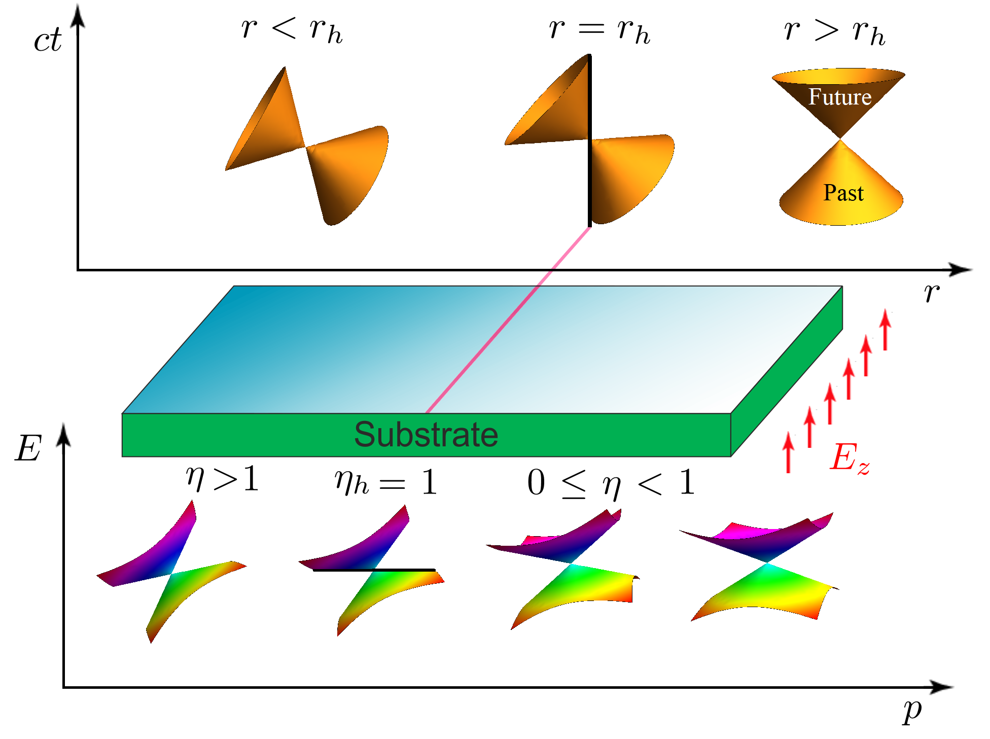
Figure 1: Schematic illustration of the low energy physics (solid state) analog of the black-hole horizon in $8Pmmn$ lattice. The strong-field region will correspond to the interior of the black-hole.

Following Volovik Nissinen and Volovik (2017); Volovik (2016a, 2018), let us view the dispersion of a tilted Dirac cone as a null-surface in a Painelevé-Gullstrand (PG) space-time,

$$ds^{2}=-v_{F}^{2}dt^{2}+(d{\boldsymbol{r}}-{\boldsymbol{v}}_{t}dt)^{2}.$$ (3)

The $v_{t}$ can have arbitrary dependence on space-time coordinates. When $v_{t}$ is inversely proportional to the radial coordinate, i.e. $\eta=v_{t}/v_{F}=r_{h}/r$ (where $r_{h}=2GM/v_{F}$ is the solid-state horizon radius), the resulting PG metric will be a coordinate transformation of celebrated Schwartzchild space-time Carroll (2003) that remains regular at the horizon Martel and Poisson (2001). In our work $v_{t}$ can be arbitrary, and we will show that it is solely controlled by the perpendicular electric field. Therefore in $8Pmmn$ borophene, the geometry of such a generic PG space-time can be engineered via engineering the space-time profile of $v_{t}$ or equivalently $\eta$. The dispersion of massless particles in this space time is given by $g_{\mu\nu}k^{\mu}k^{\nu}=0$, or equivalently, $(E-{\boldsymbol{k}}.{\boldsymbol{v}}_{t})^{2}-v_{F}^{2}k^{2}=0$ which is equivalent to the dispersion relation (2). When the tilt-velocity is allowed to depend on the radial coordinate as $v_{t}/v_{F}=r_{h}/r$, the over-tilt condition $v_{t}>v_{F}$ corresponds to $r<r_{h}$ which defines the balck-hole in this space-time geometry as in Fig. 1.

Unlike existing proposals of black-hole physics Curiel (2019) in condensed matter systems based on liquid Helium Novello et al. (2002) or Bose-Einstein condensates in three space dimensions Macher and Parentani (2009); Curtis et al. (2018), which require very low-temperature or high pressures, the $8Pmmn$ borophene sheet offers a solid-state system at ambient conditions with additional tunability to explore black-hole physics on the table top. Recent solid-state proposals in 3+1 dimensions employ the external strain Guan et al. (2017) or intrinsic inhomogeneity Huang et al. (2018) where a type-III Weyl material with $\eta=1$ (right at the horizon) can slightly change to either $\eta<1$ or $\eta>1$ (see Fig. 1). In our proposal, apart from dealing with a 2+1 dimensional space-time which makes our system a unique space-time laboratory on the table-top, the electric field offers a wide tunability which is different from slight changes induced by strain. Furthermore, being two-diemnsional allows to ”pattern” the electric field to design arbitrary 2+1 dimensional space-time.

II Results

II.1 Candidate material

As pointed out earlier, the non-symmorphic structure of the lattice is essential to produce substantial tilt in the pristine form Liu et al. (2019). Boron is the light element with the atomic number $Z=5$ which is in the left of Carbon in periodic table of elements. It has a number of structures Ezawa (2017) some of which are synthesized Mannix et al. (2015); Zhong et al. (2017a, b); Feng et al. (2016); Zhang et al. (2016a, b). We will be dealing with the $8Pmmn$ structure shown in Fig. 2 which is predicted to be stable Tang and Ismail-Beigi (2007, 2010); Zhou et al. (2014); Lopez-Bezanilla and Littlewood (2016). Earlier layered material hosting tilted Dirac cone was the $\alpha$-BEDT organic conductor Kajita et al. (2014a). The common features of $8Pmmn$ borophene apart from hosting the tilted Dirac cones Zabolotskiy and Lozovik (2016), is that the low-energy degrees of freedom in both systems is built from molecular orbitals Zhou et al. (2014) rather than the atomic orbitals. However, their essential difference is that the organic conductor is a layered material, while $8Pmmn$ borophene is an atom-thick two-dimensional material. In symmorphic structures such as graphene, the amount of tilt that can be extrinsically produced by applying an appropriate strain on it is negligible. Furthermore, the electric field tunability of the tilt parameter of borophene is not available in graphene. Therefore we are left with only one suitable choice among the present three possible 2+1-dimensional tilted Dirac cone systems. Search for other 2+1-dimensional systems with substantial intrinsic tilt deformation of the Dirac equation remains an open problem.

Figure 2: Lattice structure of $8Pmmn$ borophene: (a) top view (b) side view. Green rectangle is the unit cell.

II.2 Effective Hamiltonian

The most generic $8Pmmn$-invariant $4\times 4$ Hamiltonian in the basis of molecular orbitals, $|\psi^{c},\frac{1}{2}\rangle$, $|\psi^{v},\frac{1}{2}\rangle$, $|\psi^{c},-\frac{1}{2}\rangle$,$|\psi^{v},-\frac{1}{2}\rangle$ is given by (see SM for details),

$$H=f(\vec{k})\sigma_{0}\tau_{0}+m(\vec{k})\sigma_{0}\tau_{3}+t_{0}k_{x}\sigma_{0}\tau_{2}$$

$$+\Delta_{\rm KM}k_{y}\sigma_{3}\tau_{1}$$

$$+\sum_{i,j=1}^{2}k_{i}\sigma_{j}\epsilon_{ij}(\lambda^{R}_{0,i}\tau_{0}+\lambda^{R}_{3,i}\tau_{3})$$

$$+(\lambda_{2}\sigma_{2}+\lambda_{1}k_{x}k_{y}\sigma_{1})\tau_{2}$$

$$+\sum_{i=1}^{3}B_{i}\sigma_{i}g_{0,i}\tau_{0}+M_{i}^{\rm int}g_{3,i}\tau_{3}$$ (4)

where $f(\vec{k})=f_{0}+f_{1}k_{x}^{2}+f_{2}k_{y}^{2}$, $m(\vec{k})=m_{1}k_{x}^{2}+m_{2}k_{y}^{2}-m_{0}$ and we have used the explicit form of $\Gamma$ matrices in terms of direct product of Pauli matrices $\sigma$ (in spin-space) and $\tau$ (in molecular orbital space). $\Delta_{\rm KM}$ is spin-orbit coupling of the Kane-Mele Kane and Mele (2005)-type, $\lambda^{R}_{0,i}$ and $\lambda^{R}_{3,i}$ for $i=1,2$ are anisotropic Rashba spin-orbit coupling. $\lambda^{R}_{0,i}$ is proportional to external electric field Min et al. (2006) while $\lambda^{R}_{3,i}$ is similar to ”buckling” term of Silicene structure Ezawa (2017). $\lambda_{1},\lambda_{2}$ are forms of spin-orbit coupling which are specific to the $8Pmmn$ structure. The $\lambda$ couplings are proportional to the coordinate $z$ itself. Similarly, in the last line, we have two types of Zeeman coupling. The term containing $\tau_{0}$ are related to coupling to external field $B$, and the term containing $\tau_{3}$ is due to internal exchange fields which roots in the orbital angular momentum of the molecular orbitals involved. In both electric and magnetic field related terms, those couplings carrying the subscript $3$ which are coupled to $\tau_{3}$ arise from internal fields specific to $8Pmmn$ structure. The lack of symmetry under $z\to-z$ prevents them from vanishing.

II.3 Spin Hall effect in borophene

The first line of equation (4) is what gives the long-wave length limit in equation (1). As long as only the first line is concerned, a pair of tilted Dirac cones at $\vec{k}^{\zeta}=(0,\zeta k_{D})$ along the $\Gamma Y$ line are obtained, where $k_{D}=\sqrt{m_{0}/m_{2}}$ and $\zeta=\pm$ is the valley index. The tilt is then controlled by $f_{2}$ parameter. The second line is related to spin-orbit coupling. Generically this term generates a gap in the tilted Dirac cone spectrum. The reason is simple, because in the first line $\tau_{3}$ and $\tau_{2}$ are already used, and the second line being containing $\tau_{1}$ in two space dimensions will always generate a gap. To see this, let us define $\vec{p}=\vec{k}-\vec{k}^{\zeta}$ and linearize the above Hamiltonian when only the first two lines are present:

$$H=F_{0}\tau_{0}+F_{1}\sigma_{3}\tau_{1}+F_{2}\tau_{2}+F_{3}\tau_{3}$$ (5)

where $F_{0}=2\zeta f_{2}k_{D}p_{y}$, $F_{1}=\zeta\Delta_{\rm KM}k_{D}+\Delta_{\rm KM}p_{y}$, $F_{2}=t_{0}p_{x}$ and $F_{3}=2\zeta m_{2}k_{D}p_{y}$. The spectrum of the above Hamiltonian for two eigenvalues $\sigma_{3}=\pm 1$ (for $\uparrow$ and $\downarrow$ states) is given by

$$2\zeta f_{2}k_{D}p_{y}\pm\sqrt{\Delta_{\rm KM}^{2}(\zeta k_{D}+p_{y})^{2}+(t_{0}p_{x})^{2}+4(m_{2}k_{D}p_{y}\sigma_{3})^{2}}$$

As can be seen, the tilt is controlled by $\zeta f_{2}k_{D}$ and is therefore opposite for the two valleys. Moreover at Dirac nodes $\vec{k}^{\zeta}$, we have $\vec{p}=0$ and therefore the resulting mass term is a Haldane mass and will be given by $\zeta\Delta_{\rm KM}k_{D}$ Haldane (1988) which will give rise to SHE Tokura et al. (2019); Jungwirth et al. (2012); Manchon et al. (2015). Hydrogenation brings in some $sp^{3}$ component which enhances the spin-orbit term ($\Delta_{\rm KM}$ in our case). The valley and spin dependence of the gap lies at the core of proposal by Kane and Mele Kane and Mele (2005). Observation of this effect for hydrogenated graphene has been discussed by Balakrishnan and coworkers Balakrishnan et al. (2014). The further control parameter in the case of borophene is that in addition to the extrinsic enhancement of spin-orbit coupling ($\Delta_{\rm KM}$), one can also use the strain to manipulate $k_{D}$ Oliva-Leyva and Naumis (2013); Mañes et al. (2013).

A very important property of borophene in contrast to graphene is that, while in graphene both topologically trivial Dirac mass and topologically non-trivial Haldane mass are allowed by symmetries of the lattice, in the case of borophene, as long as it remains in the $8Pmmn$ symmetry group, the Haldane mass is the only possible form of gap. To see this, let us try to add a gap opening term proportional to $\tau_{1}$. If it is not of the $\sigma_{3}\tau_{1}$ form, then it must be proportional to $\sigma_{0}\tau_{1}=\Gamma_{45}$ which belongs to $B_{3u}$ representation (see SM) and is even with respect to time-reversal. But the basis functions in this representation are odd with respect to TR. This means that only spin-orbit coupling is able to gap out the tilted Dirac cone spectrum of $8Pmmn$ borophene. Indeed this has been confirmed by ab-initio calculations. In the case of pristine borophene where only intrinsic spin-orbit coupling exists, the spin-orbit induced gap is $\sim 0.03$ meV, while for hydrogenated borophene the buckling arising from $sp^{3}$ nature of the bonds will give extrinsic contribution to spin-orbit coupling Castro Neto and Guinea (2009) which then generates two orders of magnitude larger spin-orbit gap $\sim 2.25$ meV Fan et al. (2018). Note that, although the gap opening comes from $\sigma_{3}$ term, the two spin sub-bands corresponding to $\uparrow$ and $\downarrow$ spins remain degenerate as $\sigma_{3}^{2}=(\pm 1)^{2}=+1$. The effect of spin-orbit coupling in $8Pmmn$ group is different from e.g. $P4/nmm$ group where even spin-orbit coupling is not able to gap out the resulting two-dimensional Dirac cone Young and Kane (2015).

A further prediction of the first two lines of our effective Hamiltonian, equation (4) which maybe relevant to $8Pmmn$ crystals other than borophene is that if a material in this group happen to have $m_{0}=0$, we will have $k_{D}=0$ and therefore the Dirac cone will move to $\Gamma$ pint. This will have two consequences: (i) The gap which is controlled by Haldane mass $\zeta\Delta_{\rm KM}k_{D}$ vanishes. (ii) The tilt which is controlled by the $\zeta f_{2}k_{D}$ combination also vanishes. Therefore as $m_{0}\to 0$, the two tilted gapped Dirac spectrum with opposite tilt move towards each other, and collide at $\Gamma$ pint, whereby both gap and tilt are destroyed. Since the $\Delta_{\rm KM}$ term being related to spin-orbit coupling is non-zero for extrinsic or intrinsic reasons, the only way to diminish the Haldane mass will be to require $k_{D}=0$. But this will also diminish the tilt. In this way, the SHE and tilt are locked to each other and always go hand in hand. This suggests a possible connection between the tilt and the $Z_{2}$ index of the resulting SHE state.

II.4 Electric field effects

Now let us discuss the third and fourth line of our effective Hamiltonian, equation (4). The spin structure is of the Rashba form ${\boldsymbol{k}}\times{\vec{\sigma}}.\vec{z}$ where $\vec{z}=z\hat{z}$ is a vector perpendicular to the crystal sheet. This term being proportional to the real space coordinate $z$ is related to a linear electrostatic profile which is equivalent to a constant electric field, $E_{z}$ perpendicular to the borophene sheet. Having a Rashba spin-orbit coupling form can be potentially useful in spintronic applications Manchon et al. (2015). The origin of the electric field can be extrinsic or intrinsic. The externally applied electric field couples to both conduction and valence states on equal footing. Therefore it will be isotropic in $\tau$ space and hence will be coupled through $\tau_{0}$. This accounts for the first term in the third line where Rashba parameters $\lambda^{R}_{0,i}$ are introduced and they are related to external electric field by $E_{\rm ext}z\alpha_{i}=\lambda^{R}_{0,i}$ where $\alpha_{i}$ with $i=1,2$ accounts for the anisotropy of the crystal. In the isotropic approximation, this constant will not depend on the direction $i$. The second term $\lambda^{R}_{3,i}$ is coupled via $\tau_{3}$, meaning that it couples asymmetrically to molecular orbital degrees of freedom forming the conduction and valence bands. This can be traced back to the lack of symmetry under $z\to-z$ of the crystal in Fig. 2 which gives rise to staggered polarization pattern.

This staggered polarization when projected in the space of low-energy molecular orbitals $|\psi^{c}\rangle$ and $|\psi^{v}\rangle$, generates $\tau_{3}$ term as in the third line of equation (4). Similar arguments apply to the fourth line. Therefore couplings $\lambda^{R}_{3,i}$, $\lambda_{2}$ and $\lambda_{1}$ arise from internal polarization fields and are fixed by materials parameters. Progress in the calculation of polarization for periodic solids Resta (2002); King-Smith and Vanderbilt (1993) can be employed to obtain ab-initio estimates of these couplings for $8Pmmn$ borophene.

The matrix structure of the third line in the space of molecular orbitals is $\lambda^{R}_{0,i}\tau_{0}+\lambda^{R}_{3,i}\tau_{3}={\rm diag}(\lambda^{R}_{0,i}+\lambda^{R}_{3,i},\lambda^{R}_{0,i}-\lambda^{R}_{3,i})$. Since $\lambda^{R}_{0}$ can be externally tunned by applied electric field, it can be used to tune either of the upper or lower diagonal components to zero. In this way the the resulting (anisotropic) Rashba term will become orbital-selective Xie et al. (2014). A uniaxial strain is expected to distort the low-energy molecular orbitals whereby the intrinsic $\lambda^{R}_{3,i}$ couplings can be changed Mañes et al. (2013); Oliva-Leyva and Naumis (2013).

II.5 Tunable tilt: a tool for space-time engineering

Now we are ready to discuss the most important message of our work which is the tunning of the tilt parameter by electric fields in $8Pmmn$ borophene sheets. The role of all $\lambda$ terms in equation (4) is to generate spin-orbit gaps (see the next subsection). But since Boron is a very light element, the intrinsic spin-orbit gaps are on the scale of $0.02$ meV Fan et al. (2018). Therefore we can ignore the mass terms. To look into the velocity scales in $x$-direction we set $p_{y}=0$ in equation (9) to obtain,

$$\varepsilon_{\tau}(p_{x})=sp_{x}\sqrt{t_{0}^{2}+u^{2}+2\tau w^{2}}$$ (6)

$$u^{2}=\lambda_{1}^{2}k_{D}^{2}+\left(\lambda_{3,1}^{R}\right)^{2}+\left(\lambda_{0,1}^{R}\right)^{2}$$

$$w^{4}=\lambda_{1}^{2}k_{D}^{2}\left(\lambda_{3,1}^{R}\right)^{2}+t_{0}^{2}\left[\left(\lambda_{0,1}^{R}\right)^{2}+\left(\lambda_{3,1}^{R}\right)^{2}\right]$$

where $s=\pm 1$ are eigenvalues of $\sigma_{3}$ and $\tau=\pm 1$ refer to the eigenvalues of $\tau_{3}$ matrix. Now define the tilt and major velocity scale by $v_{t}=\frac{v_{+}+v_{-}}{2},~{}~{}~{}v_{F}=\frac{v_{+}-v_{-}}{2}$ from which we get, in the limit of very large electric fields such that $\lambda^{R}_{0,1}\gg t_{0}$ we obtain,

$$v_{tx}\approx(t_{0}^{2}+u^{2})^{1/2},~{}~{}~{}~{}v_{Fx}\approx\frac{w^{2}}{\sqrt{t_{0}^{2}+u^{2}}}$$ (7)

In this limit the major Fermi velocity $v_{Fx}$ is saturated, while $v_{tx}$ remarkable is linearly controlled by the electric field. Similarly to investigate the velocity scales related to $y$ direction, we ignore the gap and set $p_{x}=0$ which gives,

$$v_{ty}=2\zeta f_{2}k_{D}+s\lambda_{0,2}^{R},~{}~{}~{}~{}v_{Fy}=2\zeta m_{2}k_{D}+s\lambda_{3,2}^{R}$$ (8)

This again shows a linear dependence of the $v_{ty}$ to electric field, while the $v_{Fy}$ does not change by electric field.

Therefore the major Fermi velocities $v_{Fi}$ determining the solid angle subtended by the Dirac cone are essentially controlled by intrinsic parameters and intrinsic (albeit anisotropic) Rashba couplings $\lambda^{R}_{3,i}$, while the corresponding tilt velocity $v_{ti}$ is controlled by external electric field $\lambda^{R}_{0,i}$. The intrinsic Rashba spin-orbit energy scales for pristine borophene are $\lambda^{R}_{3,i}\sim 10^{-2}$ meV. By hydrogenation and introducing $sp^{3}$ component, it can be enhanced up to $\sim 2$ meV Fan et al. (2018). At energy scales well above these scales, the spin-orbit gap can be ignored, and we are essentially dealing with a gapless (two-space dimensional) Dirac node. When the external electric field is zero, the cone is given by the tilt parameter $\eta=3.4/8.0\sim 0.4$ Fan et al. (2018). By increasing the external electric field, this value will keep increasing. Beyond the point corresponding to $\eta_{h}=1$, it will be overtilted Volovik (2016b); Nissinen and Volovik (2017). The reason we have used the subscript $h$ (for ”horizon”) rather than $c$ (for ”critical”) is to emphasize gravitational analogy Nissinen and Volovik (2017); Novello et al. (2002); Volovik (2016b).

Therefore $8Pmmn$ borophene is a promising solid-state platform where a background electric field can manipulate the tilt velocity scales. The ability to tune the tile of a Dirac cone is already interesting by itself. Larger tilt enhances the effect of Landau quantizations and makes the ultra quantum limit much more accessible than the upright Dirac cone Morinari et al. (2009). Also when it comes to plasmon oscillations, the tilt gives rise to a kink in the plasmon spectrum Jalali-Mola and Jafari (2018a, b). An interesting amplification of magnetic fields by crossed electric fields can also be achieved in tilted Dirac cone systems where the effective ”tilt-boosted” magnetic fields felt in the two valleys are reciprocally related Jafari (2019).

Equipped with the gravitational analogy, $8Pmmn$ borophene can be used as a ”black-hole on the table top” : One can apply strong enough perpendicular electric field to a portion of borophene sample. The region with the strong field will correspond to overtilted Dirac cone, while the low-field region will be described by undertilted Dirac equation. The strong-field region will correspond to the interior of the black-hole, while the low-field region will correspond to the exterior of the black-hole as in Fig. 1.

Moving across the horizon in Fig. 1, corresponds to the Lifshitz transition of the Dirac dispersion which will leave a signature in superconducting correlations Li et al. (2017). Letting the electric field profile oscillate with time will cause the horizon to oscillate. This will act like a source of gravitational waves which describes the oscillatory behavior of the metric. Within Einstein equation, the ”source” determining the metric is the mass content of space time, while in our case the metric is determined by background electric field. Fixing a location for the tip of scanning tunneling microscope can detect that oscillations of the metric in the form of oscillatory superconducting correlations. Any time a distortion of space-time in the form of a ”tilt-hump” with $\eta\approx 1$ reaches the STM tip, it will detect an enhancement of superconducting correlations Li et al. (2017). Therefore the condensed matter analogue of ”gravitational waves” of our simulated space-time are the waves of superconducting correlations.

Another effect of the horizon in condensed matter applications would be that, the electron-hole pairs created by e.g., sun light near the horizon will have some chance to enter the black hole. Even a small in-plane electric field bias can encourage e.g. holes more than electrons to dive into black hole where their future light cone is limits them to $\eta>1$ region. Therefore the horizon is a barrier for the recombination of electron-hole pairs. Given the two space dimensional nature of our system, this effect may find potential applications in solar cells where reduction of electron-hole recombination is a merit.

II.6 Valley Hall Effect

Now let us discuss the physics of $\lambda$ terms which are Rashba-type and $8Pmmn$ generalizations of Rashba. Typical scale of $\lambda^{R}_{0}$ terms arising from electric fields in Germanene is $\sim 10$ meV Ezawa (2012) while in the intrinsic case $\Delta_{\rm KM}\sim 0.03$ meV Fan et al. (2018). Therefore let us ignore the Kane-Mele term, and focus on the $\lambda$-terms only. The essential role of $\lambda$ terms is to open spin-orbit gaps, whereby to generate Dirac mass for the fermions of equation (1). The effective Hamiltonian around Dirac valley labeled by $\zeta=\pm 1$ is given by ($\Delta_{\rm KM}=0,B=0$)

$$H= (F_{0}+\lambda^{R}_{0,1}p_{x}\sigma_{2}-\lambda^{R}_{0,2}p_{y}\sigma_{1}-\zeta\lambda^{R}_{0,2}k_{D}\sigma_{1})\tau_{0}$$

$$+ (F_{2}+\zeta\lambda_{1}k_{D}p_{x}\sigma_{1}+\lambda_{2}\sigma_{2})\tau_{2}$$

$$+ (F_{3}+\lambda^{R}_{3,1}p_{x}\sigma_{2}-\lambda^{R}_{3,2}p_{y}\sigma_{1}-\zeta\lambda^{R}_{3,2}k_{D}\sigma_{1})\tau_{3}$$ (9)

where $F_{\mu}$ coefficients are given below equation (5). Setting $p_{x}=p_{y}=0$, we obtain the ”gap matrix” as

$$g=-\zeta\lambda^{R}_{0,2}k_{D}\sigma_{1}\tau_{0}+\lambda_{2}\sigma_{2}\tau_{2}+\zeta\lambda^{R}_{3,2}k_{D}\sigma_{1}\tau_{3}.$$ (10)

Note that the only $\lambda^{R}_{0,2}$ and $\lambda^{R}_{3,2}$ appear in the gap matrix. The other two Rashba terms corresponding to $x$ direction, namely $\lambda^{R}_{0,1}$ and $\lambda^{R}_{3,1}$ appear as coefficients of $p_{x}$ term. Their role is to renormalize the Fermi velocity and the velocity scale associated with the tilt which was discussed in previous next subsection. Corresponding to two eigenvalues $s=\pm 1$ of matrix $\sigma_{3}$, the eigenvalues of the above matrix are

$$-d\pm\zeta\lambda^{R}_{3,2}k_{D},~{}~{}~{}+d\pm\zeta\lambda^{R}_{3,2}k_{D},~{}~{}~{}d=\sqrt{\lambda_{2}^{2}+\left(\zeta\lambda^{R}_{0,2}k_{D}\right)^{2}}.$$ (11)

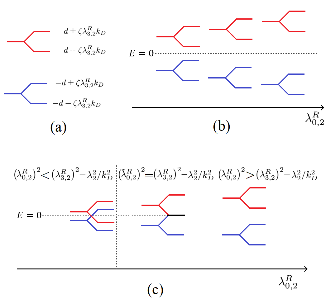
Figure 3: Schematic level diagram in the presence of external electric field.

Now there are two situations: (i) $|\lambda_{2}|>|\lambda^{R}_{3,2}|k_{D}$ and (ii) $|\lambda_{2}|<|\lambda^{R}_{3,2}|k_{D}$. These are schematically shown in Fig. 3 As can be seen from the schematic level diagram, the spectral gap in case (i) is given by $2(d-\zeta\lambda^{R}_{3,2}k_{D})$ (see Fig. 3.b). The valley symmetry is explicitly broken, which in turn will give rise to valley Hall effect. As can be seen by turning on the external field $\lambda^{R}_{0,2}$ and increasing it, the gap always increases, and the valley asymmetry becomes less important. Therefore in case (i), the valley Hall effect is decreased by turning on perpendicular electric field and increasing it. Case (ii) is more interesting. In this case the gap will be given by $-2(d-\zeta\lambda^{R}_{3,2}k_{D})$. This quantity is positive when the external electric field is absent. At a critical value of $\left(\tilde{\lambda}^{R}_{0,2}\right)^{2}=\left(\lambda^{R}_{3,2}\right)^{2}-\lambda_{2}^{2}/k_{D}^{2}$ this gap vanishes, and beyond this point, the gap changes sign (see Fig. 3.c). In either case, the valley Hall effect arising from the asymmetry between the Rashba gaps in the two valleys is present. But now by increasing the externally applied perpendicular electric field, the sign of valley Hall effect can be changed.

II.7 Magnetic field effects

The last line contains the effect of Zeeman coupling. In table II of supplementary material, we have assumed that the ”world” is composed of $8Pmmn$ crystal and the apparatus generating the $\vec{B}$. In this way, under time-reversal $\vec{B}$ changes sign, and therefore to construct TR invariant Hamiltonian for the ”world” (which is equivalent to breaking TR of the ”system”) it has to couple to appropriate $\Gamma$ matrices which are odd with respect to TR. In this way, we have obtained the last line of equation (4). The first term of the last line is similar to the standard Zeeman coupling which couples evenly to the molecular orbital degrees of freedom ($\propto\tau_{0}$). However, the second term which containing $\tau_{3}$, asymmetrically couples to orbital degrees of freedom. Similar to electric field case, the $g_{0,i}$ couplings are related to the externally applied field (or exchange field) while $g_{3,i}$ couplings are intrinsic and arise from the orbital angular momenta of the molecular orbitals involved. When the couplings are tunned to satisfy $g_{0,i}=\pm g_{3,i}$, the Zeeman coupling will be orbital selective.

To understand the physics of this line, let us assume that $\Delta_{\rm KM}\approx 0$ and $B\neq 0$,

$$H=(F_{0}+\sum_{i=1}^{3}B_{i}\sigma_{i}g_{0,i})\tau_{0}+F_{2}\tau_{2}+(F_{3}+\sum_{i=1}^{3}M_{i}^{\rm int}\sigma_{i}g_{3,i})\tau_{3}$$

The magnetic field has no effect on the Fermi and tilt velocities, as there is no term related to $B$ or $M$ in coefficients of $p_{x}$ and $p_{y}$ in Hamiltonian. Zeeman terms generation gaps as,

$$\varepsilon_{g}=s\sqrt{(B_{i}+\tau M^{\rm int}_{i})^{2}}$$ (12)

These gaps arising from magnetic field interplay with the Kane-Mele gap and will enrich the phase diagram Ezawa (2012).

III Summary and Discussion

We have obtained effective Hamiltonian of the non-symmorphic $8Pmmn$ borophene sheet which has a substantial intrinsic tilt in the spectrum of its Dirac fermions. Due to the non-symmorphic nature of the underlying lattice, a perpendicular electric field couples to the system in such a way that it can tune the tilt parameter $v_{t}=\eta v_{F}$. The tilt parameter $\eta$ on the other hand can be regarded as a parameter in the effective space-time felt by the electrons and holes of the $8Pmmn$ graphene (Fig. 1). In this analogy, the border between the high field region with overtilted Dirac cone and a low-field region with undertilted Dirac cone will correspond to a horizon. For an electron moving near the horizon the particle content of the states will be different from the one which is away from the horizon. Those approaching the horizon will feel more particle fluctuations which correspond to enhanced superconducting correlations in a superconducting proximity set up. Letting the electric fields controlling the tilt $\eta$ to dance, will act like a source of ”gravitational” waves which translate into waves of superconducting correlations. As such they can be detected as a wave of enhanced superconducting correlations in solid state spectroscopies.

The ability to engineer the metric felt by electrons promotes our borophene system as a space-time simulator, albeit in 2+1 dimensions. Given that our real world is 3+1 dimensional, our proposal offers a unique solid-state platform to explore 2+1 dimensional space-time which can not be found in cosmos.

We also discussed valley Hall effect arising from the asymmetry $\eta\to-\eta$ of the two tilts. Extrinsically enhancing the spin-orbit coupling by e.g. hydrogenation will generate spin Hall effect which would be perhaps comparable to the same effect in hydrogenated graphene Balakrishnan et al. (2013).

IV acknowledgements

We wish to thank Mehdi Torabian, Shant Baghram, Mehdi Kargarian, Mojtaba Allaei and Abolhassan Vaezi for fruitful discussion. T.F. appreciates Iman Ahmadabadi for useful discussion about the EBR. T.F. appreciates the financial support from Iran National Science Foundation (INSF) under post doctoral project no. 96015597. Z. F. was supported by Iran Science Elites Federation (ISEF) post doctoral fellowship. S. A. J. appreciates research deputy of Sharif University of Technology, grant no. G960214.

Appendix A The nonsymmorphic $8Pmmn$ group

To be self-contained, in this section we present details of the $8Pmmn$ group and its representations. The lattice structure of borophene is shown in Fig. 4. The symmetry group of Borophene is $8Pmmn$, where the $8$ stands for the number of atoms in the units cell. The $8Pmmn$ is point group number $59$ Bradley and Cracknell (2010). The generators (minimal set of elements from which all other members of the group can be constructed) are given by Bradley and Cracknell (2010); Dresselhaus et al. (2007), $\tilde{C}_{2x}=\{C_{2x}|\frac{a}{2}00\},\tilde{C}_{2y}=\{C_{2y}|0\frac{b}{2}0\},\tilde{I}=\{I|000\}$, where the notation $\{C_{2x}|{\mathbf{t}}\}$ is a nonsymmorphic element meaning the two-fold rotation $C_{2x}$ around the $x$ axis is followed by a translation $\mathbf{t}$. All other symmetry operations of the $8Pmmn$ group can be constructed from the above generators as follows: $\tilde{C}_{2z}=\tilde{C}_{2x}\tilde{C}_{2y}=\{C_{2z}|\frac{a}{2}\frac{b}{2}0\}$, $\tilde{M}_{z}=\tilde{I}\tilde{C}_{2z}=\{M_{z}|\frac{a}{2}\frac{b}{2}0\}$, $\tilde{M}_{x}=\tilde{I}\tilde{C}_{2x}=\{M_{x}|\frac{a}{2}00\}$ and $\tilde{M}_{y}=\tilde{I}\tilde{C}_{2y}=\{M_{y}|0\frac{b}{2}0\}$ Bradley and Cracknell (2010). This group has $8$ commuting elements and therefore being Abelian, admits $8$ one-dimensional irreducible representations Bunkar (1979) given in Table. 1. Extensions beyond the double-lines are related to the double group which is obtained by taking the spin of the electrons into account and that upon a $2\pi$ rotation, the spinor goes into its negative Dresselhaus et al. (2007). The double group admits two-dimensional representations which are not relevant to our minimal $4\times 4$ matrix representations of the effective Hamiltonian of borophene.

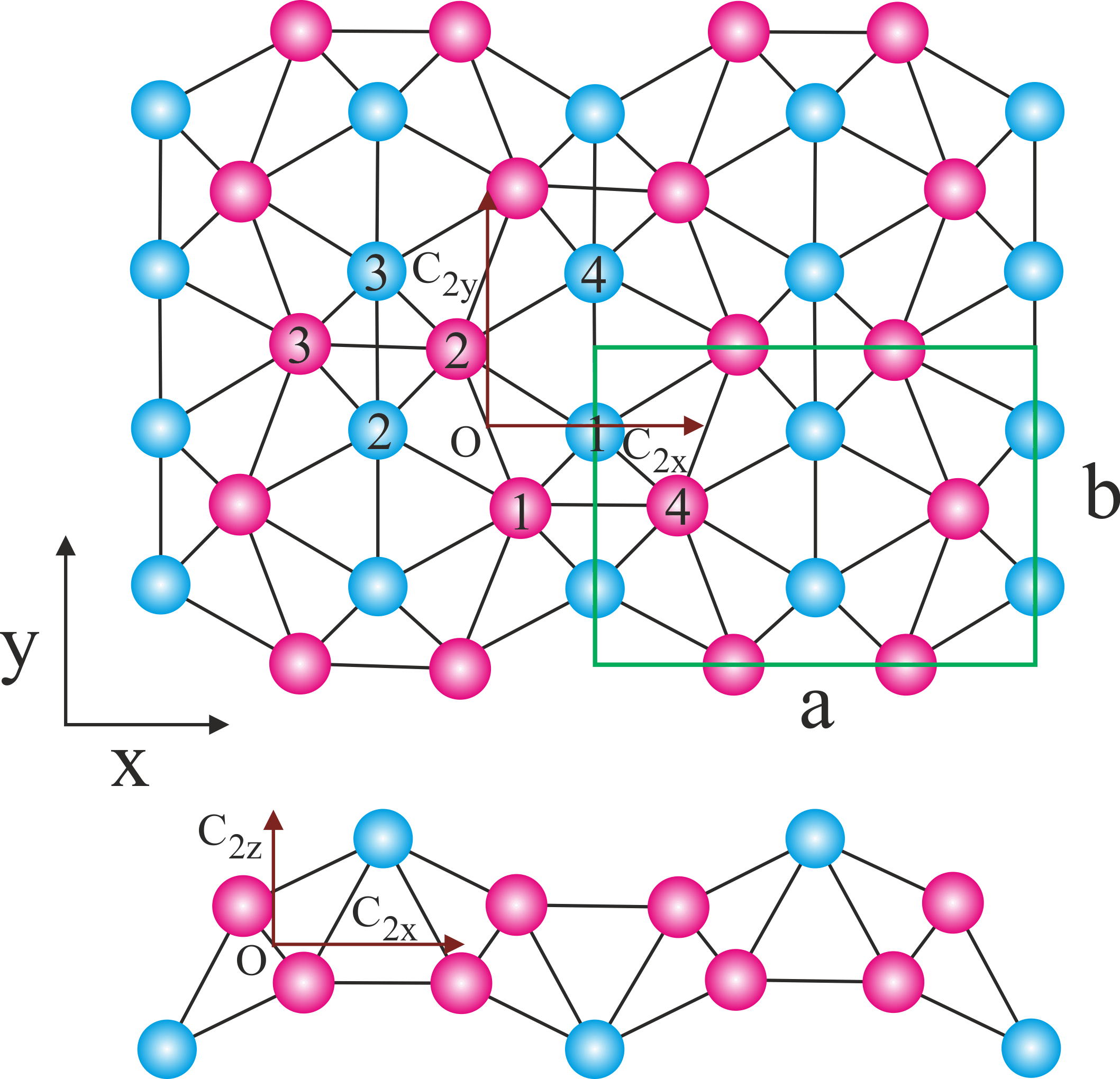
Figure 4: (Color online) Borophene lattice structure (a) top view (b) side view. The screw symmetry axes for $\tilde{c_{2x}}$, $\tilde{c_{2y}}$ and $\tilde{c_{2z}}$ indicated by brown. Green rectangular is the selected unit cell.

Nonsymmorphic elements such as ”gline planes and screw axes cause the bands to stick together on the special surface lines and planes” Kittel (1983). Following Kittel Kittel (1983) let us see how does it work for the $8Pmmn$ group. In the Brillouin zone of the system (Fig. 5) let $\psi(x,y)$ be some basis wave function on the boundary line $Z$ of the BZ. Then the screw rotation operation $\tilde{C}_{2x}$ acts as $\tilde{C}_{2x}\psi(x,y)=\psi(x+\frac{a}{2},-y)$ while the inversion $\tilde{I}$ is defined by the operation $\tilde{I}\psi(x,y)=\psi(-x,-y)$. On other hand $\tilde{M}_{x}$ acts as $\tilde{M}_{x}\psi(x,y)=\psi(-x+\frac{a}{2},y)$ which means,

$$\tilde{C}_{2x}\psi(x,y)=\tilde{M}_{x}\tilde{I}\psi(x,y)$$ (13)

Now the argument by Kittel works by showing that assumption of non-degeneracy on $Z$ line leads to contradiction Kittel (1983). So let us assume that on the $Z$ line, the representation is one dimensional. From $\tilde{I}^{2}\psi(x,y)=\psi(x,y)$ it follows that $\tilde{I}\psi(x,y)=\pm\psi(x,y)$. The same story holds for $\tilde{M}_{x}\psi(x,y)=\pm\psi(x,y)$. Therefore by Eq. (13) we must have,

$$\tilde{C}_{2x}^{2}\psi(x,y)=\tilde{M}_{x}\tilde{I}\tilde{M}_{x}\tilde{I}\psi(x,y)$$

$$=(\pm 1)^{2}(\pm 1)^{2}\psi(x,y)=\psi(x,y)$$ (14)

However from the very definition of $\tilde{C}_{2x}$ we have,

$$\tilde{C}_{2x}^{2}\psi(x,y)=\tilde{C}_{2x}\psi(x+\frac{a}{2},-y)=\psi(x+a,+y)$$

$$=e^{ik_{x}a}\psi(x,y)=e^{i\pi}\psi(x,y)=-\psi(x,y)$$ (15)

Table 1: Character table of $8pmmn$ double group

	$E$	$\tilde{c}_{2z}$	$\tilde{c}_{2y}$	$\tilde{c}_{2x}$	$\tilde{I}$	$\tilde{M}_{z}$	$\tilde{M}_{y}$	$\tilde{M}_{x}$	$CE$	$C\tilde{I}$
$A_{g}$	1	1	1	1	1	1	1	1	1	1
$A_{u}$	1	1	1	1	-1	-1	-1	-1	1	-1
$B_{1g}$	1	1	-1	-1	1	1	-1	-1	1	1
$B_{1u}$	1	1	-1	-1	-1	-1	1	1	1	-1
$B_{2g}$	1	-1	1	-1	1	-1	1	-1	1	1
$B_{2u}$	1	-1	1	-1	-1	1	-1	1	1	-1
$B_{3g}$	1	-1	-1	1	1	-1	-1	1	1	1
$B_{3u}$	1	-1	-1	1	-1	1	1	-1	1	-1
$E_{g/2}$	2	0	0	0	2	0	0	0	-2	-2
$E_{u/2}$	2	0	0	0	-2	0	0	0	-2	2

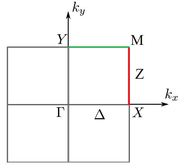
Figure 5: (Color online) Rectangular first Brillouin zone.

which contradicts Eq. (A). Note that in the the second line we have used the Bloch theorem and that on $Z$ line we have $k_{x}a=\pi$. Therefore, along the $XM=Z$ line of Fig. 5, the irreducible representations can not be one-dimensional. Now assuming that one of the states is $\psi$, again a similar argument by Kittel  shows that both $\psi$ and $\tilde{C}_{2x}T\psi$ where $T$ is the time-reversal operator, are degenerate. The same considerations apply to the $YM$ line.

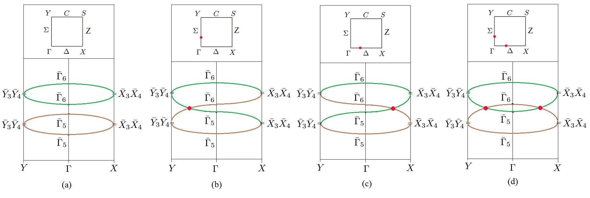
Figure 6: (Color online) Possible decomposition of elementary band representation in the presence of time reversal symmetry labeled according to notations of Bilbao crystallography server Elcoro et al. (2017). (a) the disconnected components of EBR correspond to the insulating phase of $8Pmmn$ group materials, (b) a Dirac node points along the $\Gamma Y$ path, (c) a Dirac node along the $\Gamma X$ path and (d) a pair of Dirac points along the $Y\Gamma X$ path in BZ.

A.1 elementary band representation

In this section by considering the Brillouin zone of the system, we obtain all the ways that are possible for energy bands to be connected in order to obtain realizable band structure Bradlyn et al. (2017); Cano et al. (2018); Bradlyn et al. (2018). In the band theory, the symmetry-enforced semimetal is realized when the number of electrons is a fraction of the number of connections that forms an elementary band representation (EBR). The possible candidate for semimetallic materials are identified from EBRs Bradlyn et al. (2017); Cano et al. (2018); Bradlyn et al. (2018).

The possible decomposition of elementary band representation of the $8Pmmn$ group with time reversal symmetry is illustrated in Fig. 6. As shown in Fig. 6-a the disconnected components of EBR correspond to the insulating phase of $8Pmmn$ group materials. Fig. 6-b and Fig. 6-c show a graph with connected EBR which indicate the screw-symmetry and time reversal protected topological semimetal. In these two figures (Fig. 6-b and Fig. 6-c) Dirac nodes along the $\Gamma X$ and $\Gamma Y$ are obtained. According to EBR, there is yet another possibility shown in Fig. 6-d which corresponds to two pairs of Dirac points along the $Y\Gamma X$ path in BZ. However, as will become clear in the following sections and in agreement with ab-initio calculations related to ”borophene” Zhou et al. (2014), the most general Hamiltonian constructed from irreducible representations will correspond Fig. 6-b. There can be other possible materials with the same $8Pmmn$ which may realize three other possibilities in Fig. 6.

Appendix B Molecular orbitals and effective Hamiltonian

The first known example of tilted Dirac cone material is the organic conductor $\alpha$-(BEDT-TTF)₂I₃, which is composed of molecular orbitals Kajita et al. (2014b). It was noted by Zhou and coworkers that in the case of borophene the charge density for the states at the bottom of the conduction band and top of valence band are enhanced on some bonds Zhou et al. (2014). On the other hand, ab-initio calculation of Ref. Fan et al. (2018) shows that the eigenvalues of operators $(\tilde{C}_{2x},\tilde{C}_{2y},\tilde{I})$ for bottom of conduction and top of valence band states are $(+1,+1,+1)$ and $(+1,-1,-1)$, respectively. This information is sufficient to let us construct most general molecular orbital consistent with the above eigenvalues. To do this, let us start from Fig. 4. The pink atoms correspond to ”inner” (${\rm I}$) and blue atoms correspond to ”ridge” (${\rm R}$) borons Lopez-Bezanilla and Littlewood (2016). Both type of atoms are labeled by $1,2,3,4$. As can be seen in Fig. 4, at the level of point group, we have following actions for the generators of $8Pmmn$ group: $\tilde{C}_{2x}$ replace $(1^{\rm I}\leftrightarrow 3^{\rm I},2^{\rm I}\leftrightarrow 4^{\rm I})$, $(1^{\rm R}\leftrightarrow 2^{\rm R},3^{\rm R}\leftrightarrow 4^{\rm R})$. For $\tilde{C}_{2y}$ we have $(1^{\rm I}\leftrightarrow 2^{\rm I},3^{\rm I}\leftrightarrow 4^{\rm I})$ and $(1^{\rm R}\leftrightarrow 3^{\rm R},2^{\rm R}\leftrightarrow 4^{\rm R})$. Finally $\tilde{I}$ acts as, $(1^{\rm I}\leftrightarrow 2^{\rm I},3^{\rm I}\leftrightarrow 4^{\rm I})$ and $(1^{\rm R}\leftrightarrow 2^{\rm R},3^{\rm R}\leftrightarrow 4^{\rm R})$. At the next level, depending on whether the relevant orbital in each of the above positions is $p_{x},p_{y}$ or $p_{z}$, we have:

$$\tilde{C}_{2x}\{p_{x}\}=p_{x},\tilde{C}_{2x}\{p_{y,z}\}=-p_{y,z}$$

$$\tilde{C}_{2y}\{p_{y}\}=p_{y},\tilde{C}_{2x}\{p_{x,z}\}=-p_{x,z}$$

$$\tilde{I}\{p_{x,y,z}\}=-p_{x,y,z}.$$

It should be noted that the inversion center is located at the crossing point of two screw axis as plotted in Fig. 4. Imposing the eigenvalues $(+1,+1,+1)$ and $(+1,-1,-1)$ for the conduction and valence states, we obtain the most general molecular orbitals composing the bottom of conduction band ($|\Psi^{c}\rangle$) and those at the top of valence band ($|\Psi^{v}\rangle$) as follows:

$$|\Psi^{c}_{\rm mol}\rangle\propto$$ (16)

$$\alpha\left(p_{x}^{\rm I1}-p_{x}^{\rm I2}+p_{x}^{\rm I3}-p_{x}^{\rm I4}\right)+\beta\left(p_{y}^{\rm R1}-p_{y}^{\rm R2}+p_{y}^{\rm R3}-p_{y}^{\rm R4}\right)$$

$$+\gamma\left(p_{z}^{\rm I1}-p_{z}^{\rm I2}-p_{z}^{\rm I3}+p_{z}^{\rm I4}\right)+\gamma^{\prime}\left(p_{z}^{\rm R1}-p_{z}^{\rm R2}-p_{z}^{\rm R3}+p_{z}^{\rm R4}\right)$$

$$|\Psi^{v}_{\rm mol}\rangle\propto$$ (17)

$$\alpha^{\prime}\left(p_{x}^{\rm I1}+p_{x}^{\rm I2}+p_{x}^{\rm I3}+p_{x}^{\rm I4}\right)+\alpha^{\prime\prime}\left(p_{x}^{\rm R1}+p_{x}^{\rm R2}+p_{x}^{\rm R3}+p_{x}^{\rm R4}\right)$$

$$\gamma^{\prime\prime}\left(p_{z}^{\rm I1}+p_{z}^{\rm I2}-p_{z}^{\rm I3}-p_{z}^{\rm I4}\right).$$

As can be seen the eigenvalues of $(\tilde{C}_{2x},\tilde{C}_{2y},\tilde{I})$ imply that the $p_{y}$ orbitals are absent in the valence band states. This is in agreement with Ref. Lopez-Bezanilla and Littlewood (2016). This reference further suggests that the coefficient $\beta$ of the $p_{y}$ orbitals in the conduction band is also negligible. The coefficients can not be fixed by the symmetry argument. But this is already enough to let us construct the most general Hamiltonian compatible with the above eigenvalues. We have used the subscript ”mol” to emphasize the molecular orbital nature of degrees of freedom involved in the low-energy effective theory of borophene. This should be contrasted to a graphene sheet, where atomic $p_{z}$ orbitals form the low-energy electronic degrees of freedom.

Eqns. (16) and  (17) allow us to construct the matrix representation of the generators (and hence all other members) of the $8Pmmn$ group. Let $\tau_{i},i=1,2,3$ denote the Pauli matrices acting on the space of the above molecular orbitals. $\tau_{0}$ is the unit $2\times 2$ matrix. Adding the spin structure, let $\sigma_{i}$ denote the Pauli matrices in the space of $\uparrow$ and $\downarrow$ states. Again $\sigma_{0}$ will be the unit matrix in this space. In this basis we have the following representation,

$$\tilde{C}_{2x}=i\sigma_{1}\tau_{0},~{}~{}\tilde{C}_{2y}=i\sigma_{2}\tau_{3},~{}~{}\tilde{I}=\sigma_{0}\tau_{3},T=i\sigma_{2}\tau_{0}K$$ (18)

where a tenser product $\otimes$ is understood. $T$ is the time-reversal, and $K$ is the complex conjugation. This representation is on the space of four states $|\Psi^{c}_{\rm mol},\pm\frac{1}{2}\rangle$ and $|\Psi^{v}_{\rm mol},\pm\frac{1}{2}\rangle$. In this space, the most general $4\times 4$ Hamiltonian can be written as,

$$H=d_{0}(k){\mathbbm{1}}+\sum_{i}d_{i}(k)\Gamma_{i}+\sum_{ij}d_{ij}(k)\Gamma_{ij},$$ (19)

where $\mathbbm{1}$ denotes the $4\times 4$ identity matrix and the $\Gamma$s are suitable basis in the space of $4\times 4$ matrices. One possible explicit representation is given by Liu et al. (2010),

$$\Gamma_{1}=\sigma_{x}\otimes\tau_{x}$$

$$\Gamma_{2}=\sigma_{y}\otimes\tau_{x}$$

$$\Gamma_{3}=\sigma_{z}\otimes\tau_{x}$$

$$\Gamma_{4}=1\otimes\tau_{y}$$

$$\Gamma_{5}=1\otimes\tau_{z}$$

$$\Gamma_{ij}=[\sigma_{i}\otimes\tau_{x},\sigma_{j}\otimes\tau_{x}]/2i=\epsilon_{ijk}\sigma_{k}\otimes 1$$

$$\Gamma_{i4}=[\sigma_{i}\otimes\tau_{x},1\otimes\tau_{y}]/2i=\sigma_{i}\otimes\tau_{3}$$

$$\Gamma_{i5}=[\sigma_{i}\otimes\tau_{x},1\otimes\tau_{z}]/2i=-\sigma_{i}\otimes\tau_{y}$$

$$\Gamma_{45}=[1\otimes\tau_{y},1\otimes\tau_{z}]/2i=1\otimes\tau_{x}$$ (20)

Functions $d_{0}(k)$, $d_{i}(k)$ and $d_{ij}(k)$ are polynomials in $k$. Now using Eq. (18) one can construct the effect of all symmetry operators $g$ of the $8Pmmn$ group on the above set of $\Gamma$ matrices by $g:\Gamma\to g\Gamma g^{-1}$.

The properties of $\Gamma$ matrices under the generators of $8Pmmn$ group operators and time reversal symmetry operator $T$ are given in the following. For $\tilde{C}_{2x}$ we have,

$$\tilde{C}_{2x}\Gamma_{1}\tilde{C}_{2x}=\Gamma_{1},~{}~{}\tilde{C}_{2x}\Gamma_{2}\tilde{C}_{2x}=-\Gamma_{2},~{}~{}\tilde{C}_{2x}\Gamma_{3}\tilde{C}_{2x}=-\Gamma_{3}$$

$$\tilde{C}_{2x}\Gamma_{4}\tilde{C}_{2x}=\Gamma_{4},~{}~{}\tilde{C}_{2x}\Gamma_{5}\tilde{C}_{2x}=\Gamma_{5},~{}~{}\tilde{C}_{2x}\Gamma_{45}\tilde{C}_{2x}=\Gamma_{45}$$

$$\tilde{C}_{2x}\Gamma_{15}\tilde{C}_{2x}=\Gamma_{15},~{}~{}\tilde{C}_{2x}\Gamma_{25}\tilde{C}_{2x}=-\Gamma_{25},~{}~{}\tilde{C}_{2x}\Gamma_{35}\tilde{C}_{2x}=-\Gamma_{35}$$

$$\tilde{C}_{2x}\Gamma_{14}\tilde{C}_{2x}=\Gamma_{14},~{}~{}\tilde{C}_{2x}\Gamma_{24}\tilde{C}_{2x}=-\Gamma_{24},~{}~{}\tilde{C}_{2x}\Gamma_{34}\tilde{C}_{2x}=-\Gamma_{34}$$

$$\tilde{C}_{2x}\Gamma_{12}\tilde{C}_{2x}=-\Gamma_{12},~{}~{}\tilde{C}_{2x}\Gamma_{13}\tilde{C}_{2x}=-\Gamma_{13},~{}~{}\tilde{C}_{2x}\Gamma_{23}\tilde{C}_{2x}=\Gamma_{23}$$

For $\tilde{C}_{2y}$ we obtain,

$$\tilde{C}_{2y}\Gamma_{1}\tilde{C}_{2y}=\Gamma_{1},~{}~{}\tilde{C}_{2y}\Gamma_{2}\tilde{C}_{2y}=-\Gamma_{2},~{}~{}\tilde{C}_{2y}\Gamma_{3}\tilde{C}_{2y}=\Gamma_{3}$$

$$\tilde{C}_{2y}\Gamma_{4}\tilde{C}_{2y}=-\Gamma_{4},~{}~{}\tilde{C}_{2y}\Gamma_{5}\tilde{C}_{2y}=\Gamma_{5},~{}~{}\tilde{C}_{2y}\Gamma_{45}\tilde{C}_{2y}=-\Gamma_{45}$$

$$\tilde{C}_{2y}\Gamma_{15}\tilde{C}_{2y}=\Gamma_{15},~{}~{}\tilde{C}_{2y}\Gamma_{25}\tilde{C}_{2y}=-\Gamma_{25},~{}~{}\tilde{C}_{2y}\Gamma_{35}\tilde{C}_{2y}=\Gamma_{35}$$

$$\tilde{C}_{2y}\Gamma_{14}\tilde{C}_{2y}=-\Gamma_{14},~{}~{}\tilde{C}_{2y}\Gamma_{24}\tilde{C}_{2y}=\Gamma_{24},~{}~{}\tilde{C}_{2y}\Gamma_{34}\tilde{C}_{2y}=-\Gamma_{34}$$

$$\tilde{C}_{2y}\Gamma_{12}\tilde{C}_{2y}=-\Gamma_{12},~{}~{}\tilde{C}_{2y}\Gamma_{13}\tilde{C}_{2y}=\Gamma_{13},~{}~{}\tilde{C}_{2y}\Gamma_{23}\tilde{C}_{2y}=-\Gamma_{23}$$

Under inversion they behave as,

$$\tilde{I}\Gamma_{1}\tilde{I}=-\Gamma_{1},~{}~{}\tilde{I}\Gamma_{2}\tilde{I}=-\Gamma_{2},~{}~{}\tilde{I}\Gamma_{3}\tilde{I}=-\Gamma_{3}$$ (23)

$$\tilde{I}\Gamma_{4}\tilde{I}=-\Gamma_{4},~{}~{}\tilde{I}\Gamma_{5}\tilde{I}=\Gamma_{5},~{}~{}\tilde{I}\Gamma_{45}\tilde{I}=-\Gamma_{45}$$

$$\tilde{I}\Gamma_{15}\tilde{I}=-\Gamma_{15},~{}~{}\tilde{I}\Gamma_{25}\tilde{I}=-\Gamma_{25},~{}~{}\tilde{I}\Gamma_{35}\tilde{I}=-\Gamma_{35}$$

$$\tilde{I}\Gamma_{14}\tilde{I}=\Gamma_{14},~{}~{}\tilde{I}\Gamma_{24}\tilde{I}=\Gamma_{24},~{}~{}\tilde{I}\Gamma_{34}\tilde{I}=\Gamma_{34}$$

$$\tilde{I}\Gamma_{12}\tilde{I}=\Gamma_{12},~{}~{}\tilde{I}\Gamma_{13}\tilde{I}=\Gamma_{13},~{}~{}\tilde{I}\Gamma_{23}\tilde{I}=\Gamma_{23}$$

Finally under time-reversal they are transformed as,

$$T\Gamma_{i}T^{-1}=-\Gamma_{i},~{}~{}~{}i=1,2,3,4$$

$$T\Gamma_{5}T^{-1}=\Gamma_{5}$$

$$T\Gamma_{ij}T^{-1}=-\Gamma_{ij}~{}~{}~{}T\Gamma_{i4}T^{-1}=-\Gamma_{i4}$$

$$T\Gamma_{i5}T^{-1}=\Gamma_{i5}~{}~{}~{}i.j=1,2,3$$

$$T\Gamma_{45}T^{-1}=\Gamma_{45}$$ (24)

Then using the character table 1 the $\Gamma$ matrices can be classified in terms of the irreducible representations. We have summarized the result of this procedure in table 2.

Table 2: Basis functions (polynomials up to third order) and $\Gamma$ matrices transforming in every irreducible representation. The values of $T=\pm$ denotes the signature under time reversal operation. As for the $B$ field itself, $T=-$ indicates that the TR operates on the whole world.

(basis;T)	representation	($\Gamma$ matrices;T)
{$1$,$k_{x}^{2}$,$k_{y}^{2}$ ;$+$}	$A_{g}$	{I, $\Gamma_{5}$;$+$}
{$k_{x}k_{y}z$;$+$ }	$A_{u}$	{$\Gamma_{15}$;$+$}
{$k_{x}k_{y}$;$+$}	$B_{1g}$	——
{$B_{z}$;$-$ }	$B_{1g}$	{$\Gamma_{12}$,$\Gamma_{34}$; -}
{$z$ ;$+$}	$B_{1u}$	{$\Gamma_{25}$;+}
{$B_{y}$,$zk_{x}$;$-$}	$B_{2g}$	{$\Gamma_{13}$,$\Gamma_{24}$;$-$}
{$k_{y}$,$k_{x}^{2}k_{y}$, $k_{y}^{3}$, $z^{2}k_{y}$;$-$}	$B_{2u}$	{$\Gamma_{3}$;$-$}
{$B_{x}$,$zk_{y}$;$-$}	$B_{3g}$	{$\Gamma_{14}$, $\Gamma_{23}$;$-$ }
{$k_{x}$, $k_{x}k_{y}^{2}$,$k^{3}_{x}$,$z^{2}k_{x}$;$-$}	$B_{3u}$	{$\Gamma_{4}$;$-$}
——	$A_{u}$	{$\Gamma_{1}$;$-$}
——	$B_{1u}$	{$\Gamma_{2}$;$-$}
——	$B_{2u}$	{$\Gamma_{35}$;$+$}
——	$B_{3u}$	{$\Gamma_{45}$;$+$}

The middle column denotes the irreducible representations of the $8Pmmn$ group. It turns out that all the $16$ $\Gamma$-matrices belong to one-dimensional representations of the $8Pmmn$ group. These are denoted in the right column, along with their signature under TR operation. Corresponding basis functions up to third order polynomials along with their signature under TR are given in the left column. Since none of the matrices belongs to $B_{1g}$ representation, the corresponding entry is empty. In $A_{u}$ and $B_{1u}$ representations in rows number $10$ and $11$, the basis functions can only have ”$+$” signature under the TR. So there is no basis function with ”$-$” TR signature to couple to $\Gamma_{1}$ and $\Gamma_{2}$ matrices. Similarly, in $B_{2u}$ and $B_{3u}$ irreducible representations of the last two rows, the basis functions are odd under TR, and there is no TR-even basis function to couple to $\Gamma_{35}$ and $\Gamma_{45}$ matrices. Now it is straightforward to construct invariant Hamiltonian: Simply multiply basis functions from the left column in their corresponding matrices in the right column.

Therefore the most generic $8Pmmn$-invariant $4\times 4$ Hamiltonian $|\psi^{c},\frac{1}{2}\rangle$, $|\psi^{v},\frac{1}{2}\rangle$, $|\psi^{c},-\frac{1}{2}\rangle$,$|\psi^{v},-\frac{1}{2}\rangle$ basis is given by,

$$H=f(\vec{k})\sigma_{0}\tau_{0}+m(\vec{k})\sigma_{0}\tau_{3}+t_{0}k_{x}\sigma_{0}\tau_{2}$$

$$+\Delta_{\rm KM}k_{y}\sigma_{3}\tau_{1}$$

$$+\sum_{i,j=1}^{2}k_{i}\sigma_{j}\epsilon_{ij}(\lambda^{R}_{0,i}\tau_{0}+\lambda^{R}_{3,i}\tau_{3})$$

$$+(\lambda_{2}\sigma_{2}+\lambda_{1}k_{x}k_{y}\sigma_{1})\tau_{2}$$

$$+\sum_{i=1}^{3}B_{i}\sigma_{i}g_{0,i}\tau_{0}+M_{i}^{\rm int}g_{3,i}\tau_{3}$$ (25)

where $f(\vec{k})=f_{0}+f_{1}k_{x}^{2}+f_{2}k_{y}^{2}$, $m(\vec{k})=m_{1}k_{x}^{2}+m_{2}k_{y}^{2}-m_{0}$ and we have used the explicit form of $\Gamma$ matrices in terms of direct product of $\sigma$ and $\tau$ matrices. $\Delta_{\rm KM}$ is spin-orbit coupling of the Kane-Mele Kane and Mele (2005)-type, $\lambda^{R}_{0,i}$ and $\lambda^{R}_{3,i}$ for $i=1,2$ are anisotropic Rashba spin-orbit coupling. $\lambda^{R}_{0,i}$ is proportional to external electric field Min et al. (2006) while $\lambda^{R}_{3,i}$ is similar to ”buckling” term Ezawa (2017). $\lambda_{1},\lambda_{2}$ are forms of spin-orbit coupling which are specific to the $8Pmmn$ structure. All $\lambda$ couplings are proportional to the coordinate $z$ itself, signifying that they are related to a linear potential profile. Those appearing along with $\tau_{3}$ are ”staggered” fields, while those evenly coupled to orbital degrees of freedom are ”uniform” fields which can be extrinsically applied. Similarly, in the last line, we have two types of Zeeman coupling. The term proportional to $\tau_{0}$ are related to coupling to external field $B_{i}$, and the term proportional to $\tau_{3}$ is due to internal exchange fields which roots in the orbital angular momentum of the molecular orbitals involved. In both electric and magnetic field related terms, those couplings carrying index $3$ which are coupled to $\tau_{3}$ arise from internal fields specific to $8Pmmn$ structure. The lack of symmetry under $z\to-z$ prevents them from vanishing.

References

- Novoselov et al. (2005) K. S. Novoselov, A. K. Geim, S. Morozov, D. Jiang, M. Katsnelson, I. Grigorieva, S. Dubonos, Firsov, and AA, nature 438, 197 (2005).
- Katsnelson and Kat︠s︡nelʹson (2012) M. I. Katsnelson and M. I. Kat︠s︡nelʹson, Graphene: carbon in two dimensions (Cambridge university press, 2012).
- Armitage et al. (2018) N. P. Armitage, E. J. Mele, and A. Vishwanath, Rev. Mod. Phys. 90, 015001 (2018).
- Wehling et al. (2014) T. Wehling, A. M. Black-Schaffer, and A. V. Balatsky, Advances in Physics 63, 1 (2014).
- Dresselhaus et al. (2007) M. S. Dresselhaus, G. Dresselhaus, and A. Jorio, Group theory: application to the physics of condensed matter (Springer Science & Business Media, 2007).
- Schwartz (2014) M. D. Schwartz, Quantum field theory and the standard model (Cambridge University Press, 2014).
- Peskin (2018) M. E. Peskin, An introduction to quantum field theory (CRC Press, 2018).
- Cabra et al. (2013) D. C. Cabra, N. E. Grandi, G. A. Silva, and M. B. Sturla, Phys. Rev. B 88, 045126 (2013).
- Mao et al. (2011) Y. Mao, W. L. Wang, D. Wei, E. Kaxiras, and J. G. Sodroski, ACS Nano 5, 1395 (2011), pMID: 21222462, https://doi.org/10.1021/nn103153x .
- Fan et al. (2018) X. Fan, D. Ma, B. Fu, C.-C. Liu, and Y. Yao, Phys. Rev. B 98, 195437 (2018).
- Morinari et al. (2009) T. Morinari, T. Himura, and T. Tohyama, J. Phys. Soc. Jpn. 78, 023704 (2009).
- Jalali-Mola and Jafari (2018a) Z. Jalali-Mola and S. A. Jafari, Phys. Rev. B 98, 195415 (2018a).
- Jalali-Mola and Jafari (2018b) Z. Jalali-Mola and S. A. Jafari, Phys. Rev. B 98, 235430 (2018b).
- Kajita et al. (2014a) K. Kajita, Y. Nishio, N. Tajima, Y. Suzumura, and A. Kobayashi, Journal of the Physical Society of Japan 83, 072002 (2014a).
- Nissinen and Volovik (2017) J. Nissinen and G. E. Volovik, JETP Letters 105, 447 (2017).
- Volovik (2016a) G. E. Volovik, JETP Letters 104, 645 (2016a).
- Volovik (2018) G. E. Volovik, Physics-Uspekhi 61, 89 (2018).
- Carroll (2003) S. Carroll, Spacetime and Geometry: An Introduction to General Relativity (Pearson, 2003).
- Martel and Poisson (2001) K. Martel and E. Poisson, Am. J. Phys. 69, 476 (2001).
- Curiel (2019) E. Curiel, Nature Astronomy 3, 27 (2019).
- Novello et al. (2002) M. Novello, M. Visser, and G. E. Volovik, Artificial black holes (World Scientific, 2002).
- Macher and Parentani (2009) J. Macher and R. Parentani, Phys. Rev. A 80, 043601 (2009).
- Curtis et al. (2018) J. B. Curtis, G. Refael, and V. Galitski, arXiv preprint arXiv:1801.01607 (2018).
- Guan et al. (2017) S. Guan, Z.-M. Yu, Y. Liu, G.-B. Liu, L. Dong, Y. Lu, Y. Yao, and S. A. Yang, npj Quantum Materials 2, 23 (2017).
- Huang et al. (2018) H. Huang, K.-H. Jin, and F. Liu, Phys. Rev. B 98, 121110 (2018).
- Liu et al. (2019) H. Liu, J.-T. Sun, and S. Meng, arXiv preprint arXiv:1901.10058 (2019).
- Ezawa (2017) M. Ezawa, Phys. Rev. B 96, 035425 (2017).
- Mannix et al. (2015) A. J. Mannix, X.-F. Zhou, B. Kiraly, J. D. Wood, D. Alducin, B. D. Myers, X. Liu, B. L. Fisher, U. Santiago, J. R. Guest, M. J. Yacaman, A. Ponce, A. R. Oganov, M. C. Hersam, and N. P. Guisinger, Science 350, 1513 (2015).
- Zhong et al. (2017a) Q. Zhong, J. Zhang, P. Cheng, B. Feng, W. Li, S. Sheng, H. Li, S. Meng, L. Chen, and K. Wu, Journal of Physics: Condensed Matter 29, 095002 (2017a).
- Zhong et al. (2017b) Q. Zhong, L. Kong, J. Gou, W. Li, S. Sheng, S. Yang, P. Cheng, H. Li, K. Wu, and L. Chen, Phys. Rev. Materials 1, 021001 (2017b).
- Feng et al. (2016) B. Feng, J. Zhang, Q. Zhong, W. Li, S. Li, H. Li, P. Cheng, S. Meng, L. Chen, and K. Wu, Nature chemistry 8, 563 (2016).
- Zhang et al. (2016a) Z. Zhang, E. S. Penev, and B. I. Yakobson, Nature chemistry 8, 525 (2016a).
- Zhang et al. (2016b) Z. Zhang, A. J. Mannix, Z. Hu, B. Kiraly, N. P. Guisinger, M. C. Hersam, and B. I. Yakobson, Nano letters 16, 6622 (2016b).
- Tang and Ismail-Beigi (2007) H. Tang and S. Ismail-Beigi, Phys. Rev. Lett. 99, 115501 (2007).
- Tang and Ismail-Beigi (2010) H. Tang and S. Ismail-Beigi, Phys. Rev. B 82, 115412 (2010).
- Zhou et al. (2014) X.-F. Zhou, X. Dong, A. R. Oganov, Q. Zhu, Y. Tian, and H.-T. Wang, Phys. Rev. Lett. 112, 085502 (2014).
- Lopez-Bezanilla and Littlewood (2016) A. Lopez-Bezanilla and P. B. Littlewood, Phys. Rev. B 93, 241405 (2016).
- Zabolotskiy and Lozovik (2016) A. D. Zabolotskiy and Y. E. Lozovik, Phys. Rev. B 94, 165403 (2016).
- Kane and Mele (2005) C. L. Kane and E. J. Mele, Phys. Rev. Lett. 95, 226801 (2005).
- Min et al. (2006) H. Min, J. E. Hill, N. A. Sinitsyn, B. R. Sahu, L. Kleinman, and A. H. MacDonald, Phys. Rev. B 74, 165310 (2006).
- Haldane (1988) F. D. M. Haldane, Phys. Rev. Lett. 61, 2015 (1988).
- Tokura et al. (2019) Y. Tokura, K. Yasuda, and A. Tsukazaki, Nature Reviews Physics (2019), 10.1038/s42254-018-0011-5.
- Jungwirth et al. (2012) T. Jungwirth, J. Wunderlich, and K. Olejník, Nature Materials 11, 382 EP (2012), review Article.
- Manchon et al. (2015) A. Manchon, H. C. Koo, J. Nitta, S. M. Frolov, and R. A. Duine, Nature Materials 14, 871 EP (2015), review Article.
- Balakrishnan et al. (2014) J. Balakrishnan, G. K. W. Koon, A. Avsar, Y. Ho, J. H. Lee, M. Jaiswal, S.-J. Baeck, J.-H. Ahn, A. Ferreira, M. A. Cazalilla, A. H. C. Neto, and B. Özyilmaz, Nature Communications 5, 4748 EP (2014), article.
- Oliva-Leyva and Naumis (2013) M. Oliva-Leyva and G. G. Naumis, Phys. Rev. B 88, 085430 (2013).
- Mañes et al. (2013) J. L. Mañes, F. de Juan, M. Sturla, and M. A. H. Vozmediano, Phys. Rev. B 88, 155405 (2013).
- Castro Neto and Guinea (2009) A. H. Castro Neto and F. Guinea, Phys. Rev. Lett. 103, 026804 (2009).
- Young and Kane (2015) S. M. Young and C. L. Kane, Phys. Rev. Lett. 115, 126803 (2015).
- Resta (2002) R. Resta, Journal of Physics: Condensed Matter 14, R625 (2002).
- King-Smith and Vanderbilt (1993) R. D. King-Smith and D. Vanderbilt, Phys. Rev. B 47, 1651 (1993).
- Xie et al. (2014) Z. Xie, S. He, C. Chen, Y. Feng, H. Yi, A. Liang, L. Zhao, D. Mou, J. He, Y. Peng, X. Liu, Y. Liu, G. Liu, X. Dong, L. Yu, J. Zhang, S. Zhang, Z. Wang, F. Zhang, F. Yang, Q. Peng, X. Wang, C. Chen, Z. Xu, and X. J. Zhou, Nature Communications 5, 3382 EP (2014), article.
- Volovik (2016b) G. E. Volovik, JETP Letters 104, 645 (2016b).
- Jafari (2019) S. A. Jafari, in preparation (2019).
- Li et al. (2017) D. Li, B. Rosenstein, B. Y. Shapiro, and I. Shapiro, Phys. Rev. B 95, 094513 (2017).
- Ezawa (2012) M. Ezawa, Phys. Rev. Lett. 109, 055502 (2012).
- Balakrishnan et al. (2013) J. Balakrishnan, G. K. W. Koon, M. Jaiswal, A. C. Neto, and B. Özyilmaz, Nature Physics 9, 284 (2013).
- Bradley and Cracknell (2010) C. Bradley and A. Cracknell, The mathematical theory of symmetry in solids: representation theory for point groups and space groups (Oxford University Press, 2010).
- Bunkar (1979) P. R. Bunkar, Molecular Symmetry and Spectroscopy (ACADEMIC PRESS, 1979).
- Kittel (1983) C. Kittel, Quantum theory of solids, 2nd Revised Edition (John Wiley and Sons, 1983).
- Elcoro et al. (2017) L. Elcoro, B. Bradlyn, Z. Wang, M. G. Vergniory, J. Cano, C. Felser, B. A. Bernevig, D. Orobengoa, G. Flor, and M. I. Aroyo, Journal of Applied Crystallography 50, 1457 (2017).
- Bradlyn et al. (2017) B. Bradlyn, L. Elcoro, J. Cano, M. Vergniory, Z. Wang, C. Felser, M. Aroyo, and B. A. Bernevig, Nature 547, 298 (2017).
- Cano et al. (2018) J. Cano, B. Bradlyn, Z. Wang, L. Elcoro, M. Vergniory, C. Felser, M. Aroyo, and B. A. Bernevig, Physical Review B 97, 035139 (2018).
- Bradlyn et al. (2018) B. Bradlyn, L. Elcoro, M. Vergniory, J. Cano, Z. Wang, C. Felser, M. Aroyo, and B. A. Bernevig, Physical Review B 97, 035138 (2018).
- Kajita et al. (2014b) K. Kajita, Y. Nishio, N. Tajima, Y. Suzumura, and A. Kobayashi, Journal of the Physical Society of Japan 83, 072002 (2014b).
- Liu et al. (2010) C.-X. Liu, X.-L. Qi, H. Zhang, X. Dai, Z. Fang, and S.-C. Zhang, Phys. Rev. B 82, 045122 (2010).