Chronostar: a novel Bayesian method for kinematic age determination. I. Derivation and application to the $\beta$ Pictoris moving group

Abstract

Gaia DR2 provides an unprecedented sample of stars with full 6D phase-space measurements, creating the need for a self-consistent means of discovering and characterising the phase-space overdensities known as moving groups or associations. Here we present Chronostar, a new Bayesian analysis tool that meets this need. Chronostar uses the Expectation-Maximisation algorithm to remove the circular dependency between association membership lists and fits to their phase-space distributions, making it possible to discover unknown associations within a kinematic data set. It uses forward-modelling of orbits through the Galactic potential to overcome the problem of tracing backward stars whose kinematics have significant observational errors, thereby providing reliable ages. In tests using synthetic data sets with realistic measurement errors and complex initial distributions, Chronostar successfully recovers membership assignments and kinematic ages up to $\approx 100$ Myr. In tests on real stellar kinematic data in the phase-space vicinity of the $\beta$ Pictoris Moving Group, Chronostar successfully rediscovers the association without any human intervention, identifies 15 new likely members, corroborates 43 candidate members, and returns a kinematic age of $17.8\pm 1.2$ Myr. In the process we also rediscover the Tucana-Horologium Moving Group, for which we obtain a kinematic age of $36.3^{+1.3}_{-1.4}$ Myr.

1 Introduction

With the advent of Gaia DR2 (Gaia Collaboration et al., 2018) we have access to an all-sky, magnitude complete survey that provides full 6D kinematic information for over 7,000,000 stars. Within this wealth of data reside the kinematic fingerprints of star formation events in the form of moving groups, stars that were formed in close proximity (both spatially and temporally) that have since become unbound and are now following approximately ballistic trajectories through the Galaxy. The development of an accurate and reliable method to infer the origin site of a moving group is a critical step in using kinematic information to constrain stellar ages, which in turn would allow calibration of model dependent ageing techniques. Accurate ages are important for many applications. They set the clock for circumstellar disc evolution and planet formation. Exoplanets are most easily directly imaged when they are young, so accurate ages enable better target selection for direct imaging campaigns. Accurate ages are required for calibration of massive stellar evolution models, but are nearly impossible to obtain directly due to these stars’ short Kelvin-Helmholtz contraction times; however, they can be age-dated approximately via their association with less massive members of a moving group.

However, current kinematic analysis methods have proven unable to deliver age estimates that are consistent with one another, or with other age estimators. One common kinematic approach is to estimate a traceback age by following the orbits of group members backwards through time to identify the age at which they occupied the smallest spatial volume. Ducourant et al. (2014) employ this technique to obtain a kinematic age for the TW Hydrae Association (TWA) of $7.5\pm 0.7\,\text{Myr}$. However Donaldson et al. (2016) obtain a different age of $3.8\pm 1.1\,\text{Myr}$ using the same method, a discrepancy that they attribute to Ducourant et al. not properly propagating measurement uncertainties. Mamajek & Bell (2014) review age estimates for the $\beta$ Pictoris Moving Group (henceforth $\beta$PMG) and find that traceback ages (Ortega et al. 2002, Song et al. 2003, Ortega et al. 2004) are $4\sigma$-discrepant with the combined lithium depletion boundary (LDB) and isochronal age of $23\pm 3\,\text{Myr}$; the sole exception is the traceback age of $22\pm 12\,\text{Myr}$ determined by Makarov (2007), which has such a large uncertainty that it provides little discriminatory power.

An alternative kinematic estimator is the expansion age, which one determines using a method analogous to the measurement of Hubble flow: one plots the positions of stars against their velocities in the same direction. If the stars are expanding, their positions and velocities will be correlated, and the slope of the correlation is just the inverse of the time since expansion began. Torres et al. (2006) apply this method to the $X$ positions and velocities of $\beta$PMG stars to obtain an age of $\sim 18\,\text{Myr}$. While this is less than $2\sigma$ from the combined LDB and isochronal age of $23\pm 3\,\text{Myr}$, Mamajek & Bell (2014) point out that the expansion slope is not consistent across dimensions. Indeed performing the same analysis in the $Z$ direction yields a negative slope, implying contraction rather than expansion.

The problems in current kinematic techniques likely have two distinct causes. First, the methods are not robust when applied to moving groups whose origin sites have complex structures in space or time. For example, Wright & Mamajek (2018) investigate the expansion rate of the Scorpius-Centaurus OB Association (Sco-Cen hereafter) by assuming it could be decomposed into three distinct subgroups (despite evidence that the true structure is significantly more complex, e.g. Rizzuto et al. 2015), but find that the kinematics are more consistent with contraction than expansion, so that any expansion or traceback age one might derive is meaningless. Even in cases where stars are expanding, both traceback and expansion methods are likely to yield misleading results if there is a non-negligible spread in the spatial distribution or age of formation sites.

A second problem is membership determination. In order to apply a kinematic ageing technique to a moving group, one must start with a list of its members, constructed either by hand or using an automated tool such as LACEwING (Riedel et al., 2017) or BANYAN (Gagné et al., 2018b) that assigns membership probabilities based on fits in 3D position or 6D phase space. Using hand-selected membership lists often produces results that depend significantly on which stars are included. However, with the automated methods the process is somewhat circular: the centre and dispersion of a purported moving group depends on which stars are included as probable members, but which stars are included in turn depends on the adopted centre and dispersion of the group. When one attempts a kinematic traceback using member lists determined in this fashion, the errors compound to the point where the method is not viable. Riedel et al. (2017) find that they can not determine kinematic ages for any known association, or even for a synthetic association described by a single age and a Gaussian distribution in space.

In this paper we introduce a new method called Chronostar that addresses many of the problems discussed above. Compared to existing methods, Chronostar has several advantages: (1) it simultaneously and self-consistently solves the problems of membership determination and kinematic ageing; (2) it does not assume or require that moving groups have a single, simple origin in space and time, and thus allows for a more realistic representation of the complex structure of star-forming regions; (3) it uses forward modelling rather than traceback, thereby eliminating the need for complex and uncertain propagation of observational errors. Our layout for the remainder of this paper is as follows. We present the formal derivation of our method in Section 2, and in Section 3 we test it on a variety of synthetic datasets, demonstrating that it is both robust and accurate. In Section 4 we present a simple application to the $\beta$ Pictoris Moving Group, showing that, for the first time, we are able to recover a kinematic age with tight error bars that is consistent with ages derived from other methods. We discuss Chronostar’s performance in comparison with other methods in Section 5. Finally, we summarise and discuss future prospects for our method in Section 6. The code for Chronostar can be found at https://github.com/mikeireland/chronostar.

2 Methods

2.1 Setup

Figure 1: Layout of the overall fitting algorithm to a set of stellar 6D astrometric data. We first convert the data into Cartesian coordinates $XYZUVW$, centred on the local standard of rest. We then perform an Expectation Maximisation (EM) fit (detailed in Section 2.4), initially with the number of components (described in Section 2.2) $n$ set to $1$, then subsequently incremented until the inclusion of an extra component worsens the fit, as determined by the Bayesian information criterion (BIC). As part of the maximisation step, we maximise each component’s set of parameters using Markov Chain Monte Carlo sampling, by first constructing a Gaussian distribution in 6D phase-space as defined by the parameters, then projecting it forward through time by the modelled age, before comparing it to its assigned members (see Figure 2).

Symbol	Units	Meaning
$X,Y,Z$	pc	Positional cartesian dimensions, centred on the Sun’s position projected onto the plane of the Galaxy, positive towards Galactic centre, circular rotation and Galactic North respectively.
$U,V,W$	$\,\text{km}\,\text{s}^{-1}$	Cartesian velocity dimensions, centred on the local standard of rest, with same orientation as $X,Y$ and $Z$ respectively.
$\boldsymbol{\theta}$	-	6D phase-space position in $XYZUVW$.
$\mathcal{N}(\boldsymbol{\theta};\boldsymbol{\mu},\boldsymbol{\Sigma})$	-	Evaluation of the 6D Gaussian with mean $\boldsymbol{\mu}$ and covariance $\boldsymbol{\Sigma}$ at the phase-space point $\boldsymbol{\theta}$.
$\boldsymbol{\mu}_{0}$	-	Modelled centroid of the 6D Gaussian distribution in $XYZUVW$ representing the initial kinematic distribution of a component of an association.
$t$	Myr	Modelled age of a component of an association.
$\sigma_{xyz}$	pc	Modelled standard deviation in $X$, $Y$ and $Z$ of initial distribution.
$\sigma_{uvw}$	$\,\text{km}\,\text{s}^{-1}$	Modelled standard deviation in $U$, $V$ and $W$ of initial distribution.
$\boldsymbol{\Sigma}_{0}$	-	Modelled covariance matrix of a 6D Gaussian distribution in $XYZUVW$ representing the initial kinematic distribution of a component of an association, constructed from $\sigma_{xyz}$ and $\sigma_{uvw}$.
$C$	-	A component modelled as a 6D Gaussian in phase-space defined by 9 parameters: initial phase-space centroid ($x_{0},y_{0},z_{0},u_{0},v_{0},w_{0}$), initial standard deviations in position and velocity space ($\sigma_{xyz},\sigma_{uvw}$) and time since becoming gravitationally unbound, $t$.
$p(d|M)$	-	The likelihood (unscaled probability) of seeing data point $d$ assuming that $d$ was drawn from the modelled distribution $M$.
$\mathbf{f}(\boldsymbol{\theta},t)$	-	Abstracted function from galpy that numerically integrates the orbit of $\boldsymbol{\theta}$ through the Galactic potential as a function of time $t$.
$\Omega_{i,k}$	-	The overlap integral of the $i$th star with the $k$th component. We calculate this by integrating over the convolution of the two associated 6D Gaussians.
$\mathbf{Z}$	-	Two-dimensional array of membership probabilities with a row for each star and a column for each component.
$w_{k}$	-	Expected fraction of stars belonging to component $k$. We calculate this by summing the $k$th column of $\boldsymbol{Z}$, and normalising by the total number of stars.

Table 1: Variables and parameters used in Section 2.

Our ultimate goal is to find the most likely kinematic description of an association’s origin, such that evolving it through time by its modelled age to its current-day distribution, best explains the observed kinematic distribution of the association’s members. In this section we detail our Bayesian approach to finding the best kinematic description of a stellar association by modelling its origins as the sum of Gaussians in 6D Cartesian phase-space with independent ages, means, and covariance matrices. We refer to each Gaussian as a component, and for the simplified models presented here, each component has the same standard deviation in each position dimension, and the same standard deviation in each velocity dimension. We define the origin of an association as the point in time at which stars become gravitationally unbound and begin moving ballistically through the Galaxy. We approximate the initial positions and velocities to be uncorrelated with one another, but as the association evolves in time those quantities will become correlated – consequently the covariance matrix, and in particular the terms within it describing position-velocity covariance, are functions of time. We fit these components to a set of observed stars by maximising the overlap between the observed stellar position-velocity information, including the full error distribution and its covariances, and the Gaussian that describes the current-day structure of a component in phase-space. We include an assessment of membership probability as part of this analysis. We decide how many components to use to fit a given set of stars by comparing the likelihood of the best fit in each case using the Bayesian Information Criterion (BIC). The BIC is a metric that balances the likelihood against a term that takes into account the number of parameters used to build the model. This term penalises the BIC (Schwarz 1978) as more parameters are included, which lowers the chance of overfitting the data (see Equation 14 and surrounding text for details). We provide Table 1 as a quick reference for the variables and parameters introduced throughout this section.

We begin this section with a top-down description of the algorithm (Figure 1). We must first decide how many components to use in our fit. A priori we do not know how many components are required to describe an association and so we run the following algorithm iteratively, incrementing the number of components each time, halting when the extra component yields a worse BIC value. For a given component count we use the Expectation Maximisation (EM) algorithm (e.g. McLachlan & Peel 2004) to simultaneously find the best parameters of each of the model components as well as the relative membership probabilities of the stars to each component. After initialisation of the model parameters, EM iterates through the Expectation step (E-step) and the Maximisation step (M-step) until convergence is reached. The E-step consists of calculating membership probabilities to not only each of the components but also to the background field distribution. The M-step utilises the membership probabilities to find the best parameters for each component through the maximisation of an appropriate likelihood function.

We now describe the model bottom up. We begin with the parametrisation of a single component’s origin as a spherical Gaussian (Section 2.2) and how we evolve this initial distribution to its current-day distribution. Next we summarise the Bayesian approach to computing the likelihood function (Section 2.3) for a single component. Finally we incorporate multiple Gaussian components using the EM algorithm, as well as the background distribution, which is critical for accounting for interlopers.

Figure 2: A basic schematic detailing how a single Gaussian component is fitted to stellar data. The red points represent stellar data at current-day (e.g., as measured by Gaia DR2) with $2\sigma$ uncertainties denoted by ellipses. The grey ellipse and cross depict the modelled initial distribution, a 6D Gaussian with mean $\boldsymbol{\mu}_{0}$ and covariance matrix $\boldsymbol{\Sigma}_{0}$. The fitting process projects the initial distribution forward by the component’s modelled age which generates the current-day distribution with mean $\boldsymbol{\mu}_{c}$ and covariance matrix $\boldsymbol{\Sigma}_{c}$, depicted by the blue ellipse and cross respectively. The orbital trajectory is denoted by the grey arc, with arrows denoting travel forward through time. For simplicity, we only show the $Z-W$ slice through the 6D phase-space but Chronostar makes use of the full 6D phase-space information.

The basic data on which our method will operate are a set of stars taken from Gaia DR2 (Gaia Collaboration et al., 2018). For the purposes of this paper we focus on stars in and around known associations, but in future work the same algorithm can be applied to search for new associations and moving groups. We transform the 6D astrometry of each star into 6D phase-space data $XYZUVW$, which describes the position and velocity of the star in Galactic coordinates as described in Table 1. In addition to the central values for each star, we have an associated set of measurement errors encapsulated by a covariance matrix. We use the transforms from Johnson & Soderblom (1987) to create a Jacobian from observed astrometry space to Cartesian $XYZUVW$ space then use this to transform the covariance matrices (similar to the process detailed in Appendix A). For the spatial coordinate origin we choose a point that coincides with the projection of the Sun onto the Galactic plane (the Sun being 25 pc above it) and whose velocity coordinate origin is given by the local standard of rest (LSR) as given by (Schönrich et al., 2010). For convenience we label this as $\boldsymbol{\theta}_{LSR}=[0,0,-25,-11.1,12.24,-7.25]$ with units as given in Table 1, denoting our coordinate system origin with respect to the Sun. We apply this offset to the data to translate the initially heliocentric data to our chosen coordinate system.

2.2 Modelling a Single Component

As stated earlier, we use a spherical 6D Gaussian distribution to model the origin of a component. We define the kinematic origin of a collection of stars as the approximation of some precise time and place when the stars become gravitationally unbound. A bound set of stars forms an ellipsoid in both position space and velocity space, with no correlation between the three pairs of position and velocity dimensions ($X-U$, $Y-V$ and $Z-W$). We refer to these three planes as mixed-phase planes henceforth. We further simplify matters by approximating the ellipsoid as spherical, thereby removing all correlations between any dimensions. We explore the validity of these assumptions in the discussion.

We parametrise the origin of a component as a Gaussian in 6D phase-space $\boldsymbol{\theta}=[x,y,z,u,v,w]$ with mean $\boldsymbol{\mu}_{0}$ representing the vector of expectation values in each dimension:

$$\boldsymbol{\mu}_{0}=[x_{0},y_{0},z_{0},u_{0},v_{0},w_{0}].$$ (1)

To satisfy the criteria stated above we parametrise the covariance matrix $\boldsymbol{\Sigma}_{0}$ as:

$$\boldsymbol{\Sigma}_{0}=\begin{bmatrix}\sigma_{xyz}^{2}&0&0&0&0&0\\ 0&\sigma_{xyz}^{2}&0&0&0&0\\ 0&0&\sigma_{xyz}^{2}&0&0&0\\ 0&0&0&\sigma_{uvw}^{2}&0&0\\ 0&0&0&0&\sigma_{uvw}^{2}&0\\ 0&0&0&0&0&\sigma_{uvw}^{2}\\ \end{bmatrix}.$$ (2)

Note, that since we restrict our model to be separately spherical in both position and velocity space we can denote the initial standard deviation in each position axis (i.e. the radius of the association) as $\sigma_{xyz}$ and the initial velocity dispersion in each velocity axis as $\sigma_{uvw}$. Hence we can express the probability density associated with each component as a Gaussian distribution over $\boldsymbol{\theta}$:

$$\mathcal{N}(\boldsymbol{\theta};\boldsymbol{\mu}_{0},\boldsymbol{\Sigma}_{0})=\frac{\exp\big{[}-\frac{1}{2}(\boldsymbol{\theta}-\boldsymbol{\mu}_{0})^{T}\boldsymbol{\Sigma}_{0}^{-1}(\boldsymbol{\theta}-\boldsymbol{\mu}_{0})\big{]}}{\sqrt{(2\pi)^{6}|\boldsymbol{\Sigma}_{0}|}}.$$ (3)

In order to relate the distribution of a component to observed stellar data we require the phase-space values of both the component model and the stellar data to be evaluated at the same time. We transform the distribution of a component from its origin (parametrised by $\boldsymbol{\mu}_{0}$ and $\boldsymbol{\Sigma}_{0}$) forward through the Galactic potential by its modelled age $t$, to its current-day distribution, another Gaussian described by $\boldsymbol{\mu}_{c}$ and $\boldsymbol{\Sigma}_{c}$, i.e. $\mathcal{N}(\boldsymbol{\theta};\boldsymbol{\mu}_{c},\boldsymbol{\Sigma}_{c})$ (see Figure 2). Using galpy (Bovy, 2015) to calculate orbits, we transform the shape of the Gaussian by considering the orbital projection of the distribution as a transformation between coordinate frames. We use galpy’s model MWPotential2014 as our model for the Galactic potential, but we show in Appendix B that choosing other plausible potentials does not lead to large differences in the results. We can thus calculate the current-day distribution by performing a first-order Taylor expansion about $\boldsymbol{\mu}_{0}$, and generating the current-day covariance matrix $\boldsymbol{\Sigma}_{c}$ under the approximation that this coordinate transformation is linear (details in Appendix A).

2.3 Fitting approach

Now that we have the means to get the current-day distribution of a component from its modelled origin point, we can use a Bayesian approach to generate a probability distribution of the model’s parameter space, which will allow us to identify each parameter’s most likely value and associated uncertainty. As is standard with a Bayesian approach, we write the posterior probability distribution of the model parameters ($C=\{\boldsymbol{\mu}_{0},\boldsymbol{\Sigma}_{0},t\}$) given the data as the product of the prior probabilities with the likelihood function:

$$p(C|D)\propto p_{\text{prior}}(C)p(D|C).$$ (4)

The prior ($p_{\text{prior}}$) represents our initial guess at the parameters in the absence of data, for example a restriction that the initial spread, dispersion and approximate mass of the system be super-virial (see Section 2.5 for details). The likelihood function $p(D|C)$ is simply the probability density of the data given the model.

In our context the data $D$ are composed of a set of $N$ stars $\{s_{1},s_{2},\dots,s_{n}\}$ that are candidate members of a component $C$, each with full 6D kinematic information. From the method described in Section 2.2 we produce a current-day distribution ($\boldsymbol{\mu}_{c}$, $\boldsymbol{\Sigma}_{c}$) from the model component parameters. We interpret the current-day Gaussian as the probability density of finding a member of $C$ at phase-space position $\boldsymbol{\theta}$. If measurements were infinitely precise this would be $\mathcal{N}(\boldsymbol{\theta};\boldsymbol{\mu}_{c},\boldsymbol{\Sigma}_{c})$ and the likelihood function for a set of $N$ stars drawn independently would simply be $p(D|C)\propto\prod_{i}^{N}\mathcal{N}(\boldsymbol{\theta}_{i};\boldsymbol{\mu}_{c},\boldsymbol{\Sigma}_{c})$. However, measurements of $\boldsymbol{\theta}_{i}$ have finite errors, which we take to be Gaussian, described by the probability distribution $\mathcal{N}(\boldsymbol{\theta};\boldsymbol{\mu}_{i},\boldsymbol{\Sigma}_{i})$, where $\boldsymbol{\mu}_{i}$ is the central estimate and $\boldsymbol{\Sigma}_{i}$ is the covariance of measurement errors. The likelihood product therefore becomes the product of convolutions of the Gaussian for component $C$ with the Gaussians describing the error ellipse for each star:

$$p(D|C)\propto\prod_{i=1}^{N}\int\mathcal{N}(\boldsymbol{\theta};\boldsymbol{\mu}_{i},\boldsymbol{\Sigma}_{i})\mathcal{N}(\boldsymbol{\theta};\boldsymbol{\mu}_{c},\boldsymbol{\Sigma}_{c})\,d\boldsymbol{\theta}\equiv\prod_{i=1}^{N}\Omega_{i,c}$$ (5)

where $\boldsymbol{\mu}_{i}$ and $\boldsymbol{\Sigma}_{i}$ are the central estimate and covariance matrix for the $i$th star respectively, and

$$\Omega_{i,c} = \frac{\exp\left[-\frac{1}{2}\left(\boldsymbol{\mu}_{i}-\boldsymbol{\mu}_{c}\right)^{T}\boldsymbol{\Sigma}_{i,c}^{-1}\left(\boldsymbol{\mu}_{i}-\boldsymbol{\mu}_{c}\right)\right]}{\sqrt{\left(2\pi\right)^{6}\left|\boldsymbol{\Sigma}_{ic}\right|}}$$ (6)

$$\boldsymbol{\Sigma}_{i,c} = \boldsymbol{\Sigma}_{i}+\boldsymbol{\Sigma}_{c}.$$ (7)

Equation 6 is the standard result for the convolution of $N$-dimensional Gaussians; note that, in the limit of no errors ($\boldsymbol{\Sigma}_{i}\rightarrow\mathbf{0}$), the result trivially reduces to $\Omega_{i,c}=\mathcal{N}(\boldsymbol{\mu}_{i};\boldsymbol{\mu}_{c},\boldsymbol{\Sigma}_{c})$ as described above. For convenience in what follows, we shall refer to $\Omega_{i,c}$ as the overlap integral of star $i$ with component $C$.

2.4 Fitting many components with the Expectation Maximisation algorithm

We now describe how to extend our formalisation so as to incorporate multiple Gaussian components, i.e. a Gaussian Mixture Model. Our model $M$ is a linear combination of $K$ components $\{C_{1},C_{2},\ldots,C_{k}\}$, and has the probability distribution function (PDF):

$$p(\boldsymbol{\theta}|M)=\sum\limits_{k=1}^{K}w_{k}\mathcal{N}(\boldsymbol{\theta};\boldsymbol{\mu}_{k},\boldsymbol{\Sigma}_{k}),$$ (8)

where $w_{k}$ is the weighting of each component such that $\sum_{k}w_{k}=1$. Intuitively $w_{k}$ is the expected fraction of stellar members belonging to component $k$. We calculate $w_{k}$ by summing the $k$th column of $\boldsymbol{Z}$ (defined below) and normalising by the total number of stars.

To simplify the maximisation of the likelihood function, the common approach is the Expectation Maximisation (EM) algorithm (McLachlan & Peel, 2004). There are many derivations of this algorithm, but for convenience we provide a brief summary. The central problem in mixture models is how to assign particular stars to particular components. EM addresses this by introducing a so-called hidden variable $\boldsymbol{Z}$ that tracks each star’s membership probabilities. $\boldsymbol{Z}$ is a matrix of $N$ rows (for each star) and $K$ columns (for each component). Each entry is a decimal number between $0$ and $1$ such that each row sums exactly to $1$. In this way the $ik$th element of $\boldsymbol{Z}$ is the probability that the $i$th star is a member of the $k$th component.

The expectation step (E-step) and maximisation step (M-step) have a circular dependency: one cannot know the membership probabilities without a fit to the components, and one cannot fit the components without knowing which stars are members. This is solved by, after a carefully chosen initialisation (described below), the algorithm alternating between the E-step (evaluating $\boldsymbol{Z}$) and the M-step (maximising each component’s likelihood function) until convergence is achieved. We can initialise this method by either using membership probabilities from the literature to guess our $\boldsymbol{Z}$, or by using fits to the distribution from the literature to guess the model parameters for the origin. We defer a more detailed discussion of how we initialise our fits to Section 2.7.

The E-step is the calculation of $\boldsymbol{Z}$, for a fixed set of components. The relative probability that star $i$ is a member of component $k$ with properties $C_{k}$ is given by its overlap integral with that component scaled by the component weight $w_{k}$, so the total probability that it is a member of component $k$ is

$$Z_{ik}=\frac{w_{k}\Omega_{i,k}}{\sum_{j=1}^{K}w_{j}\Omega_{i,j}},$$ (9)

where we use $\Omega_{i,k}$ to denote the overlap integral (Equation 6) evaluated using $\boldsymbol{\mu}_{c}=\boldsymbol{\mu}_{k}$ and $\boldsymbol{\Sigma}_{c}=\boldsymbol{\Sigma}_{k}$, i.e., using the central location and covariance matrix for component $k$.

The M-step maximises the likelihood function for fixed membership probabilities. By the introduction of $\boldsymbol{Z}$, the likelihood function becomes separable, allowing us to maximise each component’s contribution in isolation.

The likelihood function for each component is the same as the likelihood function evaluated for a single component (Equation 5), modified so that each star is weighted by the probability that it is a member:

$$p(D|C_{k},\boldsymbol{Z})\propto\prod_{i=1}^{N}(w_{k}\Omega_{i,k})^{Z_{ik}}$$ (10)

In the M-step, we use Markov Chain Monte Carlo (MCMC) (implemented by Foreman-Mackey et al. 2013 as emcee) to find the maximum likelihood values of $\boldsymbol{\mu}_{k}$ and $\boldsymbol{\Sigma}_{k}$ given the likelihood function $p(D|C_{k},\boldsymbol{Z})$ and the priors we place on $C_{k}$ (see below). We reset $\boldsymbol{\mu}_{k}$ and $\boldsymbol{\Sigma}_{k}$ to these maximum likelihood values and then return to the E-step for another iteration. The algorithm continues in this manner until converged, which we take to be when the previous iteration’s best fit parameters all fall within the central 70th percentile of the new fit’s respective posterior distribution.

2.5 Priors

Our Bayesian treatment of data requires a prior on the parameters $t_{k}$, $\boldsymbol{\mu}_{k,0}$ and $\boldsymbol{\Sigma}_{k,0}$ that describe each component. We first discuss our non-informative priors. We have a uniform prior on $t_{k}$ and each element in $\boldsymbol{\mu}_{k,0}$. The covariance matrix $\boldsymbol{\Sigma}_{k,0}$ is parametrised by only two values, $\sigma_{xyz}$ and $\sigma_{uvw}$, both of which are standard deviations. Since standard deviations are by definition restricted to be positive, the natural non-informative prior is uniform in $\ln\sigma$ rather than in $\sigma$ itself, which corresponds to $p_{\text{prior}}(\sigma)\propto 1/\sigma$. Therefore, our prior on $\boldsymbol{\Sigma}_{k,0}$ is

$$p_{\text{prior}}(\boldsymbol{\Sigma})\propto p_{\text{prior}}(\sigma_{xyz})p_{\text{prior}}(\sigma_{uvw})\propto\frac{1}{\sigma_{xyz}\sigma_{uvw}}.$$ (11)

We also add an informative prior regarding the dynamical state of purported origin sites. In testing we found that there is a mild degeneracy shared by the initial spatial volume of an association and its age, whereby some fits would collapse to an extremely small $\sigma_{xyz}$. This is unphysical, since such a tightly packed association would have been gravitationally bound and thus would not have dispersed in the first place. To counter this, we introduce a prior on the virial ratio $\alpha$ of our components, which we approximate as

$$\alpha=\frac{2\sigma_{uvw}^{2}\sigma_{xyz}}{GM},$$ (12)

where $M$ is the mass of the proposed component and $G$ is the gravitational constant. The mass of the association is not precisely known, since often the masses of individual stars are constrained only poorly, and our lists of candidate members are magnitude-limited and thus likely omit a significant number of low-mass stars. As a very rough estimate we adopt $M=nM_{\odot}$ for the purpose of computing $\alpha$, where $n$ is the number of stars in a proposed component. This amounts to assuming solar mass stars. We apply a prior with a Gaussian distribution on the natural logarithm of $\alpha$ with a mean of $2.1$ and a standard deviation of $\sigma_{\alpha}=$ $1.0$. We select these values such that the mode of the corresponding log-normal distribution occurs at $\alpha=3$. We find that smaller values of $\sigma$_α smoothly increase the fitted age when applied to real data as the fit prioritises more compact origins regardless of the data, whilst the age fit converges for $\sigma_{\alpha}\geq 1$.

2.6 Characterising field stars

For any proposed member of an association there is always a chance it is not truly a member, but rather an interloper that happens to share similar kinematic properties. We label these stars as field stars, and call the PDF of all field stars the background distribution. We use the background distribution to consider the probability that a star is a member of the background, and thus properly quantify the star’s membership probability to our association fits.

We determine our background distribution, which is held fixed, as follows. We select all Gaia DR2 stars with radial velocities and parallax errors better than 20% ($n$=6,376,803 stars), and then transform the data into Galactic cartesian coordinates ($XYZUVW$) as described in Section 2.1 . We estimate the background PDF shape in these coordinates using a Gaussian Kernel Density Estimator (KDE) to approximate a continuous PDF. The KDE we use represents the PDF as a sum of Gaussians centred on each of the $n$ input data points; these Gaussians have a covariance matrix equal to the covariance matrix of the input data set, scaled down by the square of a dimensionless factor called the bandwidth. To be precise, we estimate the background stellar density at a point $\boldsymbol{\theta}$ in parameter space as

$$p(\boldsymbol{\theta})=\sum_{i}\mathcal{N}(\boldsymbol{\theta};\boldsymbol{\mu}_{i},h^{2}\boldsymbol{\Sigma}_{G}),$$ (13)

using notation from Equation 3, where the sum runs over the $n$ stars in the Gaia DR2 catalog with acceptably small errors, $\boldsymbol{\Sigma}_{G}$ is the covariance matrix of this catalog, $\boldsymbol{\mu}_{i}$ is the $XYZUVW$ position of star $i$, and $h$ is the bandwidth. We determine $h$ using Scott’s Rule (Scott, 1992):

$$h=n^{-1/(d+4)}$$

where $d=6$ is the number of dimensions, resulting in a bandwidth of $\approx 0.2$.

We treat the background as simply another component in our multi-component fits, i.e., in a fit with $K$ components, the parameter $\boldsymbol{Z}$ is an $N\times(K+1)$ matrix, with the final column $K+1$ giving the probability that a given star is a background star rather than a member. Our treatment of the background differs from that of other components only in that the background is static and does not have any parameters that can change, so the overlap integral between it and each star $\Omega_{i,K+1}$, is a constant that may be computed once at the beginning of our calculation and then stored for use when needed. We further note that the background is essentially constant over scales in $XYZ$ and $UVW$ comparable to the sizes of measurement uncertainties, and thus we can approximate the overlap integrals $\Omega_{i,K+1}$ as simply the value of the background evaluated at the central position and velocity estimates for each star.

2.7 Initialisation and adding components

Each run of Chronostar begins with a single component, which is described by nine scalar quantities: the six components of the central phase-space position $\boldsymbol{\mu}_{0}$, the initial spatial and velocity dispersions $\sigma_{xyz}$ and $\sigma_{uvw}$, and the age $t$. We initialise an MCMC search for the maximum likelihood in the nine-dimensional space these parameters describe by placing walkers randomly around a central starting guess, which is that the components of $\boldsymbol{\mu}_{0}$ are equal to the mean of the stellar data to which we are fitting, $\sigma_{xyz}=20$ pc, $\sigma_{uvw}=7\,\text{km}\,\text{s}^{-1}$, and $t=3$ Myr. We then run the MCMC algorithm to maximise the likelihood function as described in Section 2.4, stopping when we reach convergence. At this point we have predicted posterior probability distributions for all nine quantities.

To trial an alternative two-component fit, we must specify a starting guess for the parameters of each of the two components, which will serve as starting points about which to distribute initial MCMC walker positions. We choose these starting guesses as follows. For each proposed component, we take our starting guesses for $\sigma_{xyz}$ and $\sigma_{uvw}$ to be equal to the maximum posterior probability value derived from the one-component fit. We set the starting time guesses for our two proposed components equal to the 16th and 84th percentile values of the posterior probability distribution for $t$ from the one-component fit. Finally, we set our starting guess for the phase-space position $\boldsymbol{\mu}_{0}$ of each of the two trial components such that their current-day positions match the current-day centroid position of the maximum posterior probability value for the one-component fit. From these starting guesses, we run the EM algorithm as described in Section 2.4, stopping when we converge. We then compute the BIC for the one-component versus the two-component fit using the following formula:

$$\color{blue}\text{BIC}=\ln{(n)}k-2\ln{\mathcal{L}},$$ (14)

where $n$ is the expected number of stars assigned to the components, $k$ is the number of parameters, and $\mathcal{L}$ is the evaluated likelihood. If the two-component BIC is inferior to the one-component result, we stop and accept the one-component result. If not, we accept the two-component fit, and consider the possibility of adding a third component.

The procedure for going beyond two components is much the same as for going from one to two: we initialise a search by splitting an existing component into its 16th and 84th percentile ages, setting our central guesses for the initial phase-space positions and dispersions exactly as we did when going from one to two components. The primary complication is that there is no obvious means to identify which existing component should be split in order to yield the best fit. Thus Chronostar explores all possible splits, carries out EM to find the posterior probability for each possibility, then selects the best option between these and the previous fit to one fewer components based on the BIC. We stop adding components when the fit with $N$ components has a superior BIC compared to any of the possible fits using $N+1$ components.

We caution that this procedure does not necessarily guarantee the identification of the best possible fit, especially when the number of components is relatively large. As is usual with MCMC over high-dimensional spaces (a fit to $N$ components has $9N$ dimensions), there is in general no way to guarantee that the true global maximum likelihood has been found. However, Section 3.3 demonstrates that even this basic approach successfully decomposes complex associations with multiple components.

The time taken to complete a fit is strongly dependent on the number of components required, but also depends on the number of stars and the age of the components. Each EM iteration takes on average 500-1000 MCMC steps per component. The number of EM iterations needed for convergence can vary from about 30 iterations (in the case where there is a clear sub-component needing characterisation) to upwards of 150 iterations (where the introduced component has not identified a separate distinct over-density). Simple arrangements, such as the multi-component tests we present in the next section, require only $\sim 10$ hours for convergence running on a workstation or a single node of a cluster. A blind fit to $\sim 2000$ stars will take upwards of a week on the same hardware. In the case of our $\beta$PMG fit (see Section 4), we ran the fit with 19 threads (1 per each of the 18 walkers plus one master thread) and the computation took about a week to converge. Due to these limitations, if Chronostar were to fit to all of Gaia, the data would need to be parceled into subsets of a few thousand stars at a time.

3 Testing Chronostar with synthetic data

We investigate the reliability and accuracy of our fitting approach by testing it on an extensive suite of 1080 synthetic single-component associations, three scenarios with multiple components, a set of stellar kinematics taken from a star formation simulation (Federrath 2015; Federrath et al. 2017), and a two-component association within a uniform background. We describe each of these tests in turn in the following sections.

3.1 Single-component analysis

Our first test is the simplest, and uses as its mock data single components constructed from the same distributions we have assumed can be used to describe real associations. Thus we consider origin sites that are spherical in both position and velocity space, and are parametrised by 5 values: age $t$ (i.e., how many years have passed since becoming unbound), $\sigma_{xyz}$, the standard deviation in each position dimension, $\sigma_{uvw}$, the velocity dispersion or standard deviation in each velocity dimension, $n$, the number of stars drawn from the distribution, and $\eta$, which characterises the uncertainty of the observed current-day properties as described below. The purpose of this test is to ensure that our code can recover input data whose properties match our assumptions, and to characterise the level of accuracy we can expect in this optimal case.

We use our chosen parameters to construct a synthetic data set in several steps, which we explain in more detail below: (1) we use $t$, $\sigma_{xyz}$, and $\sigma_{uvw}$ to compute the starting centroid position $\mu_{0}$ and covariance matrix $\boldsymbol{\Sigma}_{0}$ for our synthetic association; (2) we use $\boldsymbol{\mu}_{0}$ and $\boldsymbol{\Sigma}_{0}$ plus the specified number of stars $n$ to create a set of synthetic initial positions and velocities, which we then integrate forward by time $t$ to produce a set of synthetic current-day positions and velocities; (3) we add synthetic errors, whose sizes are parameterised by $\eta$, to yield a set of “observed” stars on which we run the Chronostar code.

Step (1) is to compute $\mu_{0}$ and $\boldsymbol{\Sigma}_{0}$. For the latter we set $\boldsymbol{\Sigma}_{00}=\boldsymbol{\Sigma}_{11}=\boldsymbol{\Sigma}_{22}=\sigma_{xyz}^{2}$ and $\boldsymbol{\Sigma}_{33}=\boldsymbol{\Sigma}_{44}=\boldsymbol{\Sigma}_{55}=\sigma_{uvw}^{2}$, following the assumption that our initial conditions are spherical distributions; all off-diagonal components of $\boldsymbol{\Sigma}_{0}$ are zero. For the former, we choose a starting position so that the current-day centroid position of our synthetic association matches that of Lower Centaurus-Crux (LCC), $\boldsymbol{\mu}_{\text{LCC}}=[50,-100,25,1.1,7.76,2.25]$ (see Table 1 for units) by integrating an orbit backwards through time for the desired age $t$, beginning at the desired current-day centroid $\boldsymbol{\mu}_{c}$. In other words: $\mathbf{f}(\boldsymbol{\mu}_{0},t)=\boldsymbol{\mu}_{\text{LCC}}$, where $\mathbf{f}(\boldsymbol{\mu}_{0},t)$ is the function that maps an initial position $\boldsymbol{\mu}_{0}$ to a final position $\boldsymbol{\mu}$ after orbiting a time $t$ through the Galactic potential. This choice ensures the synthetic associations are all at the same heliocentric radius thus preserving consistency with measurement uncertainties that are distance dependent.

Step (2) is drawing $n$ stars from a 6D Gaussian distribution with centroid $\mu_{0}$ and covariance matrix $\boldsymbol{\Sigma}_{0}$. We then integrate these stars forward through the Galactic potential for a time $t$. We convert the current-day position of each star from Cartesian Galactic coordinates to astrometric coordinates (RA, DEC, $\mu_{\rm RA}$, $\mu_{\rm DEC}$, parallax and radial velocity).

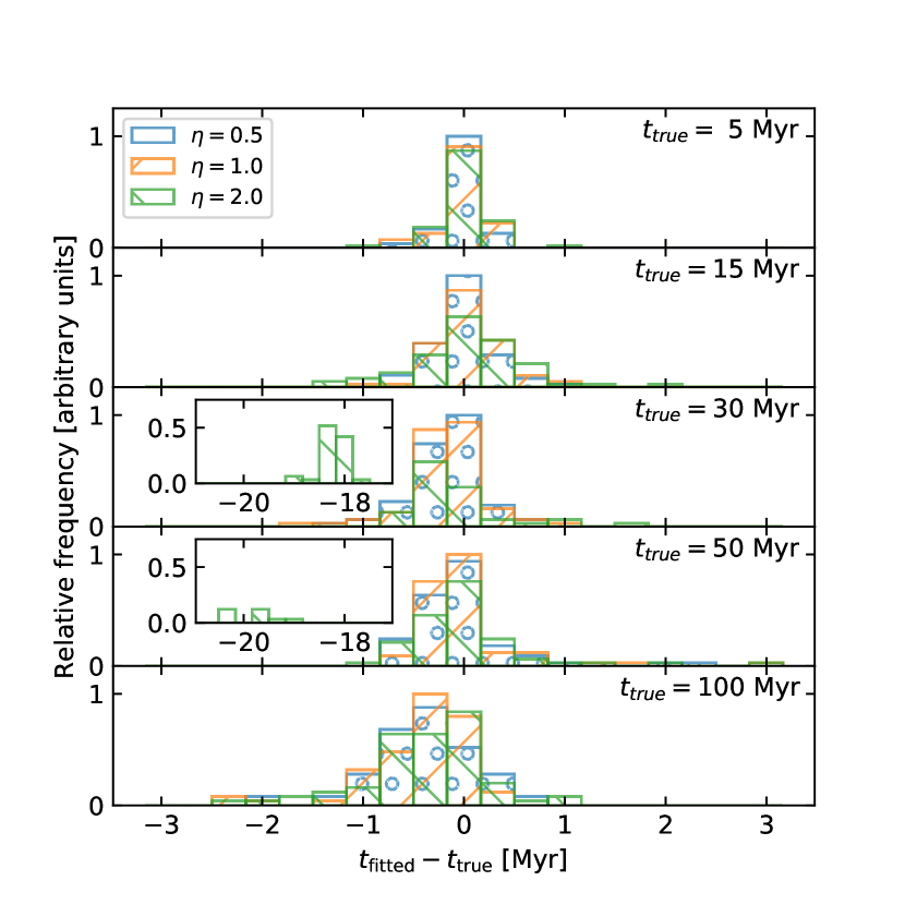
Figure 3: Histograms of residuals $t_{\text{fitted}}-t_{\text{true}}$ resulting from application of Chronostar to 1080 synthetic associations, grouped by true age (panels, increasing from top to bottom) and degree of measurement uncertainty (histograms in each panel). The catastrophic failures (featured in the insets) all cluster around 20 Myr, which is equal to the quarter period of vertical oscillations through the Galactic plane.

Figure 4: Same as Figure 3, except that we show the distribution of normalised residuals $(t_{\rm fitted}-t_{\rm true})/\sigma_{\rm fitted}$ rather than the distribution of raw residuals. For comparison, the black lines in each panel show Gaussian distributions with zero mean and unit variance, scaled such that the area under the curve matches the area under the $\eta=0.5$ histogram in each panel, and thus shows the distribution of normalised residuals we would expect if the true posterior PDF were Gaussian. We do not include the catastrophic failures in this figure.

Step (3) is to add synthetic errors. We use the median uncertainties of Gaia DR2 to inform our artificial measurement uncertainties. Of all the Gaia DR2 stars with radial velocities and parallax uncertainty better than 20%, the median uncertainties for parallax, proper motion and radial velocity are $0.035$ mas, $0.05$ mas yr^-1 and 1 km s^-1 respectively. We set the uncertainties on our synthetic data by multiplying these values by a dimensionless scale factor $\eta$, so that the parallax uncertainty is $0.035\eta$ mas, the proper motion uncertainty is $0.05\eta$ mas yr^-1, and the radial velocity uncertainty is $1\eta$ km s^-1. For each synthetic star, we add a random offset to its astrometric coordinates chosen by drawing from a Gaussian distribution of the specified size.

We generate 1080 synthetic associations by creating four realisations for each possible combination of the parameters:

$$\text{age},\,t =[5,15,30,50,100]\,\text{Myr},$$

$$\text{radius},\,\sigma_{xyz} =[1,2,5]\,\text{pc},$$

$$\text{velocity dispersion},\,\sigma_{uvw} =[1,2]\,\text{km}\,\text{s}^{-1},$$

$$\text{star count},\,n =[25,50,100],$$

$$\text{error scaling},\,\eta =[0.5,1,2].$$

We choose this range of parameters to be broadly representative of known or claimed moving group origin sites. However, the maximum values of $\sigma_{uvw}$ and $t$ for which we test deserve special mention, because they are driven in part by the limitations of our method. In deriving the likelihood function we have approximated the time evolution of the PDF of phase-space density with a linear transformation, and we show below that this approximation breaks down for association ages $\gg 100$ Myr, or velocity dispersions $\gg 2$ km s^-1.

For each synthetic association we run Chronostar using a single component; the output of the run is a set of MCMC walker positions in the space $(t,\boldsymbol{\mu}_{0},\sigma_{xyz},\sigma_{uvw})$. From these positions, we define $t_{\rm fitted}$ as the median $t$ coordinate of the walkers, and the corresponding fit uncertainty $\sigma_{\rm fitted}$ as half the difference between the 16th and 84th percentiles of $t$.

Figure 3 shows the distribution of raw residuals, $t_{\rm fitted}-t_{\rm true}$ (where $t_{\rm true}$ is the true age used to generate the synthetic data set) that we obtain from our experiment, and Figure 4 shows the corresponding normalised residuals, $(t_{\rm fitted}-t_{\rm true})/\sigma_{\rm fitted}$; in both cases the data are grouped by values of $t_{\rm true}$ and $\eta$. The raw residuals characterise the absolute accuracy of the method, while the distribution of normalised residuals characterise the accuracy of the error estimate it returns.

We find that, except for a small number of catastrophic failures that are easy to spot and discussed below, Chronostar recovers the correct ages to accuracies of $\sim 1$ Myr almost independent of $t_{\rm true}$ or $\eta$. There is a systematic bias toward younger ages that increases with $t_{\rm true}$, reaching a maximum net offset of $\sim 0.3\,\text{Myr}$ at $t_{\rm true}=100\,\text{Myr}$. We attribute this offset to the associations’ minor yet potential departures from the linear regime. The normalised residuals show distributions that are close to Gaussians with unit dispersion, indicating that the error distribution for our method is close to Gaussian, and that the returned $\sigma_{\rm fitted}$ is an accurate estimate of the true uncertainty. Again we see a slight bias toward younger ages that worsens for older $t_{\text{true}}$.

It may seem surprising that the age fits have an uncertainty so robust to $t_{\rm true}$. However ultimately the uncertainty of the age fit depends on how accurately Chronostar fits the correlation in the three mixed phase-space planes ($X-U$, $Y-V$ and $Z-W$), as these are the signatures of expansion. The stars mostly remain in the linear regime so these correlations are linear regardless of the age, therefore the reliability of the age fit is almost independent of age.

Figure 3 shows that our method catastrophically fails for a small number of cases where the true age is 30 or 50 Myr, and the error normalisation is $\eta=2$ (i.e., double the fiducial errors of Gaia measurements). In these cases, the fitted ages consistently fall short by about $20\,\text{Myr}$. This is a consequence of a degeneracy in the $Z-W$ plane. The matter density in the Galaxy is reasonably constant with $\approx 100$ pc of the Galactic plane (formally, for our standard model of the Galactic potential, the density at 100 pc is 85% of the midplane density), making the vertical restoring force close to linear in a star’s distance from the midplane, and thus similar to that of a simple harmonic oscillator. Consequently, each star in our synthetic associations has nearly the same period in the $Z$ direction, and thus for a particular current-day distribution of stellar positions and velocities there is a degeneracy between two possible starting states: stars could have started at similar heights but a wide range of velocities, or with a small range of velocities but a large variation in starting heights. The phase-space distribution of the stellar population in the $Z-W$ plane is therefore uncorrelated at multiple distinct epochs, separated by a quarter of the vertical oscillation period, which is $\approx 20$ Myr. Our catastrophic failure mode consists of the MCMC walkers settling into the first of these many degenerate minima that yields a reasonable fit in other phase-space dimensions. This failure mode only occurs for errors larger than usual for Gaia, because for smaller errors, constraints in the phase-space components that lie in the Galactic plane are sufficient to break the degeneracy in the out-of-plane directions. Thus, these failures are not a concern for practical applications, as long as the relative uncertainties for the majority of stars in question do not significantly exceed 100% that of Gaia.

3.2 Stars with realistic initial kinematics

In the previous section, all our synthetic associations had initial conditions that matched our assumptions (spherical, uncorrelated initial distribution; instantaneous gravitational unbinding). Here we consider a much more realistic initial stellar distribution by using stellar positions and velocities drawn from a simulation of star formation. The simulation we use is the run referred to as case “GTBJR” in Onus et al. (2018); its initial conditions and physics are identical to the “GvsTMJ” case presented in Federrath (2015), which includes turbulence, magnetic fields and jet feedback, but with the addition of radiation feedback as implemented in Federrath et al. (2017). The simulation tracks the collapse of a molecular cloud in a $2$ pc cube with periodic boundaries. In the simulation, stars are represented by sink particles, and for this test we take the positions and velocities of the sink particles in the final snapshot of the simulation as the initial positions and velocities of synthetic stars. As in the previous tests, we choose the absolute position and velocity of the stars in Galactic coordinates such that their current-day central position and velocity match that of LCC. We project the stars forward through time for $20$ Myr, ignoring any gravitational interactions between them, convert their positions and velocities to astrometric coordinates, and add random errors with a distribution equal to our fiducial Gaia DR2 median uncertainty ($\eta=1$; see Section 3.1). We then run Chronostar on the resulting synthetic data set.

Chronostar retrieves an age of $20.1\pm 0.2$ Myr, demonstrating that, in this instance, approximating the initial kinematic distribution of the association as spherically Gaussian is a sufficiently accurate approximation. Figure 5 shows the current and starting positions of the stars, along with the fit, in 4 different 2D projections ($X-Y$, $X-U$, $Y-V$ and $Z-W$). We see that the current-day fit provides a good match to the current-day position and velocity, and the corresponding fit to the origin falls within 3 pc of the true average initial position of the stars. One particularly noteworthy feature of this plot is that the correct fit is recovered despite the fact that, due to the relatively large uncertainties in the current-day kinematic properties of the stars, an attempt to trace the stars back in time by integrating their orbits does not show any significant amount of convergence. Thus attempts to reconstruct these stars’ origin point by looking for a minimum volume or similar, the approach used in traceback methods, would be unlikely to succeed.

We also note that the reconstruction strongly favours a single-component fit to this data set. Following the procedure outlined above, after finding a single component fit, Chronostar attempted a two-component fit. However, the BIC of the single-component fit, 546.5, is significantly better than that of the best two-component fit, 576.5.

Figure 5: Results from our test using synthetic stars drawn from a star formation simulation (Federrath 2015; Federrath et al. 2017). Panels show the positions of stars at formation 20 Myr ago (grey squares) and at the current-day (blue circles) in several different 2D projections of the 6D phase-space. Faint ellipses around the current-day positions show the error distributions for the synthetic measurement. The dashed red ellipse shows the best-fit current-day distribution retrieved by Chronostar; a similar best-fit ellipse for the origin point is also plotted in solid red. Red lines show the trajectory of the centre of the distribution, with arrows pointing forwards through time. Grey lines show the trajectories for selected current-day stars traced back from that star’s central estimate by 20 Myr. Note that, due to the relatively large uncertainties, these trajectories show minimal convergence in $X-U$ and $Y-V$ planes despite being traced back to their true seeded age. This is not the case for the trajectories in the $Z-W$ plane, which do indeed show convergence in $Z$. This is a consequence of the almost linear restoring force in the $Z$ direction, resulting in stars having similar periods. See Section 3.1 for further discussion. We note that our choice of a co-rotating reference frame introduces added motion in the $X$ and $Y$ dimensions due to the Coriolis force. As a consequence orbits in the $X-U$ plane curve towards larger values of $X$ despite having $U$ values around $-2\,\text{km}\,\text{s}^{-1}$.

3.3 Multiple components

Our next tests increase the complexity by introducing data sets with multiple components, arranged so that they have significant overlap in position, velocity, or both with incorporated observational uncertainties equal to our fiducial Gaia DR2 median uncertainty ($\eta=1$). The goal is to test Chronostar’s ability to separate such overlapping sets of stars. We initialise each fit in the default way as described in Section 2.4.

In the following text, for convenience we will refer to stars being assigned to components. We remind the reader that Chronostar does not assign discrete memberships but rather utilises continuous, probabilistic memberships. However, for convenience of plotting and discussion we will describe a star as being assigned to the component for which Chronostar gives the highest membership probability.

3.3.1 Four distinct components

The first test features four components, each containing 30 - 80 stars, that have distinct ages from 3 to 13 Myr yet have current-day distributions that overlap when viewed solely in position space or solely in velocity space. However, because these components have different ages, they are separable in joint position-velocity space (e.g., in the $Z-W$ plane). We give the full set of initial parameters for each component, and the best fits to them that Chronostar retrieves, in Table 2. We also show the current-day positions of the stars, and Chronostar’s fits to them, in two 2D projections of 6D phase-space in Figure 6.

Chronostar successfully fits the ages, initial positions, and dispersions of each component, and correctly classifies the memberships of all 200 stars, despite the fact that the four components overlap in multiple dimensions. The reason it is able to accomplish this separation becomes clear if we examine panel (b) of Figure 6, which shows the distribution of stars, and our fits to them, in the $Z-W$ plane. Consider the ellipses in (b) in order of ascending age (C, D, B, A): the angle that the semi-major axes of each component makes with the vertical increases systematically with age. In the $Z-W$ plane these angles rotate with time, completing a full rotation after 80 Myr. Similar rotation occurs with time in the $X-U$ and $Y-V$ planes (not shown), but with a different period. Chronostar is able to separate four components, despite their overlap in both position and velocity, because position-velocity correlations provide a sensitive measure of age since expansion.

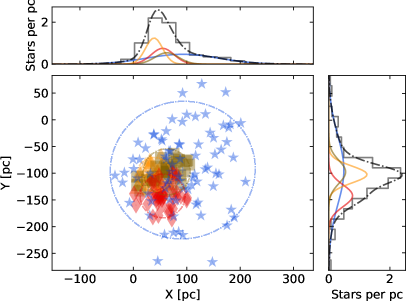
(a)

(b)

Figure 6: Results from our test using four distinct components with distinct ages but overlapping current-day positions. Panels show the positions of stars at current-day in several different 2D projections of the 6D phase-space. Faint ellipses around the current-day positions show the error distributions for the synthetic measurement but are often smaller than the data points. The dashed ellipses show the best-fit current-day distributions retrieved by Chronostar for each component; see Table 2 for the numerical values of the true and fitted parameters of each component. Marker styles show the component to which each star truly belongs, while marker colours show the component to which Chronostar assigns that star; colours and symbols match in all cases because in this test Chronostar assigns all stars correctly. Flanking plots show the 1D projection of densities in each dimension. In these plots, histograms show the distribution of synthetic stars, while curves show the probability densities for Chronostar’s best fit, which colour indicating component. The grey histogram and black line show the sum of all components.

Table 2: Parameters for our test using four distinct components with distinct ages but overlapping current-day positions. For each parameter, the “True” value is the input value used to construct the synthetic data, while the “Fit” value is the 50th percentile value for the posterior PDF returned by Chronostar, with error bars indicating the ranges from the 16th to 50th and 50th to 84th percentiles. The quantity we report for the “Fit” value of number of stars (nstars) is the sum of the membership probabilities for that component in the final, converged output of the EM algorithm.

	Component A		Component B		Component C		Component D
	True	Fit	True	Fit	True	Fit	True	Fit
$x_{0}$ [pc]	$274.8$	$267.2^{+7.2}_{-6.8}$	$132.8$	$120.7^{+7.0}_{-6.4}$	$98.0$	$99.9^{+3.8}_{-4.1}$	$125.5$	$123.8^{+3.3}_{-3.1}$
$y_{0}$ [pc]	$220.4$	$216.7^{+5.2}_{-5.3}$	$85.0$	$62.2^{+9.9}_{-9.9}$	$-46.8$	$-48.0^{+3.0}_{-3.1}$	$-52.2$	$-54.3^{+1.9}_{-2.0}$
$z_{0}$ [pc]	$-55.6$	$-51.6^{+2.4}_{-2.4}$	$11.4$	$18.0^{+3.9}_{-4.1}$	$45.6$	$48.3^{+3.0}_{-2.9}$	$59.6$	$57.7^{+2.6}_{-2.7}$
$u_{0}$ [$\,\text{km}\,\text{s}^{-1}$]	$-17.3$	$-17.4^{+0.6}_{-0.6}$	$-12.5$	$-11.5^{+0.5}_{-0.5}$	$-21.8$	$-22.7^{+0.6}_{-0.6}$	$-12.4$	$-11.8^{+0.6}_{-0.6}$
$v_{0}$ [$\,\text{km}\,\text{s}^{-1}$]	$-25.1$	$-25.1^{+0.6}_{-0.6}$	$-22.7$	$-23.3^{+0.4}_{-0.4}$	$-18.4$	$-18.6^{+0.6}_{-0.6}$	$-8.2$	$-7.6^{+0.6}_{-0.6}$
$w_{0}$ [$\,\text{km}\,\text{s}^{-1}$]	$2.6$	$1.8^{+0.5}_{-0.6}$	$7.8$	$7.6^{+0.3}_{-0.3}$	$-14.6$	$-15.0^{+0.6}_{-0.6}$	$-9.0$	$-8.9^{+0.6}_{-0.6}$
$\sigma_{xyz}$ [pc]	$20.0$	$19.4^{+1.0}_{-1.0}$	$10.0$	$9.6^{+0.8}_{-0.7}$	$10.0$	$9.4^{+0.6}_{-0.5}$	$7.0$	$7.8^{+0.7}_{-0.6}$
$\sigma_{uvw}[\,\text{km}\,\text{s}^{-1}]$	$5.0$	$4.9^{+0.2}_{-0.2}$	$2.0$	$2.0^{+0.1}_{-0.1}$	$5.0$	$4.4^{+0.3}_{-0.2}$	$3.0$	$3.0^{+0.3}_{-0.2}$
age [Myr]	$13.0$	$12.7^{+0.3}_{-0.3}$	$10.0$	$9.0^{+0.5}_{-0.5}$	$3.0$	$3.0^{+0.2}_{-0.2}$	$7.0$	$6.9^{+0.3}_{-0.3}$
nstars	80	80.00	40	40.00	50	50.00	30	30.00

3.3.2 Two components with shared trajectory

The second test uses two components with distinct ages of 7 and 10 Myr, but with origin points carefully selected such that the centroids of their current-day distributions are identical. This gives each association an identical orbital trajectory, which results in two distributions that overlap in every possible 2D projection of the 6D phase-space. This scenario presents a challenge to our fitting approach as there is no separation between the components along any dimension. The only distinction between the two components is the tilt or degree of correlation in the mixed-phase (i.e., position-velocity) planes. We give the full parameters of the two components used in this test, and the fits to them derived by Chronostar, in Table 3, and we show two projections of phase-space in Figure 7. Chronostar recovers the ages of both of our overlapping components within a $0.2$ Myr uncertainty. Only 6 stars (blue triangles in Figure 7) of 120 are misclassified, corresponding to a success rate of 95%, which is consistent with the mean membership probability that Chronostar estimates for all stars to their correct component: 94.3%. Thus Chronostar not only returns the correct assignment for the great majority of stars, it provides an accurate estimate of the confidence level of the assignments as well.

(a)

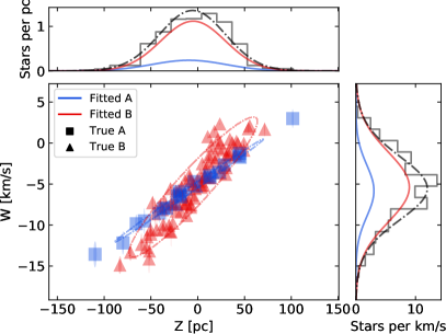
(b)

Figure 7: Results from our test using two components with distinct ages but with identical current-day centroids in both position and velocity. See caption to Figure 6 for an explanation of figure details. Note that 6 stars (blue triangles) are misclassified corresponding to a success rate of 95%, which is consistent with the mean membership probability that Chronostar estimates for all stars with respect to their correct component: 94.3%.

Table 3: Parameters for our test using two components with distinct ages but with identical current-day centroids in both position and velocity. See caption to Table 2 for an explanation of the meaning of various table entries.

	Component A		Component B
	True	Fit	True	Fit
$x_{0}$ [pc]	$179.7$	$179.4^{+2.6}_{-2.7}$	$129.5$	$128.0^{+2.3}_{-2.3}$
$y_{0}$ [pc]	$59.1$	$57.7^{+0.9}_{-0.9}$	$19.5$	$16.0^{+2.2}_{-2.1}$
$z_{0}$ [pc]	$46.1$	$46.2^{+0.6}_{-0.5}$	$34.1$	$31.8^{+1.2}_{-1.3}$
$u_{0}$ [$\,\text{km}\,\text{s}^{-1}$]	$-16.2$	$-15.8^{+0.9}_{-0.9}$	$-14.3$	$-14.2^{+0.5}_{-0.5}$
$v_{0}$ [$\,\text{km}\,\text{s}^{-1}$]	$-16.4$	$-17.6^{+0.9}_{-0.9}$	$-17.8$	$-17.6^{+0.5}_{-0.5}$
$w_{0}$ [$\,\text{km}\,\text{s}^{-1}$]	$-3.6$	$-4.5^{+0.9}_{-0.9}$	$-4.3$	$-4.6^{+0.5}_{-0.5}$
$\sigma_{xyz}$ [pc]	$2.0$	$1.9^{+0.3}_{-0.2}$	$10.0$	$10.3^{+0.5}_{-0.5}$
$\sigma_{uvw}[\,\text{km}\,\text{s}^{-1}]$	$5.0$	$4.4^{+0.4}_{-0.3}$	$5.0$	$4.9^{+0.2}_{-0.2}$
age [Myr]	$10.0$	$9.9^{+0.1}_{-0.1}$	$7.0$	$6.8^{+0.1}_{-0.1}$
nstars	20	23.90	100	96.10

3.3.3 Two components against a uniform background

The third test uses two components with distinct ages of $12$ and $25\,\text{Myr}$ and star counts of 50 and 40, along with a top-hat PDF background with density $10^{-7}[\,\text{pc}\,\text{km}\,\text{s}^{-1}]^{-3}$, chosen to be representative of the density of Gaia DR2 stars in the vicinity of $\beta$PMG (see Section 2.6 for details). We refer to the two Gaussian components as an association, and to the third component as the background. We set the bounds of the top-hat PDF representing the background to be twice the extent of the association in each dimension, and centre it on the mid-range of the association stars. The resulting bounds of the top-hat PDF are:

$$X =(-61.4,197.6)\,\text{pc},$$

$$Y =(-205.5,12.6)\,\text{pc},$$

$$Z =(-58.1,56.8)\,\text{pc},$$

$$U =(-16.5,-4.8)\,\text{km}\,\text{s}^{-1},$$

$$V =(-25.4,-13.9)\,\text{km}\,\text{s}^{-1},$$

$$W =(-9.9,-0.5)\,\text{km}\,\text{s}^{-1}.$$

We draw the true kinematics of 810 stars from this distribution as this achieves the desired overall density. It is straightforward for Chronostar to identify the association as it is a prominent over-density in both position and velocity space. The challenge lies in how Chronostar handles the membership boundaries of an association against a ubiquitous, fixed background distribution.

We give the full parameters of the two components of the association used in this test, and the fits to them derived by Chronostar, in Table 4, and we show two projections of phase-space in Figure 8. Chronostar satisfactorily deduces memberships, with only 3 (of 810) background stars misclassified as being part of the association, and only 5 (of 90) association stars misclassified as part of the background. Thus the success rate is $91.4$%. This is similar to the mean membership probability returned by Chronostar of all component stars to their true component of origin: 89.2%. If we include the membership probabilities of the misclassified background stars to the background, the mean membership probability is 86.6%. In either case, we see both that Chronostar’s membership assignments are reasonably accurate, and, as importantly, that the level of confidence it returns in those assignments is accurate as well.

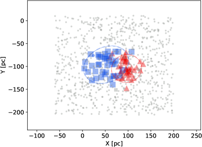
(a)

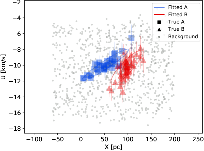
(b)

Figure 8: Results from our test using two components combined with a fixed, uniform background. See caption to Figure 6 for an explanation for figure details. Grey circles show positions of background stars that are correctly classified as part of the background. Grey square and triangular markers show stars that are in fact part of one of the two components of the association, but that are incorrectly classified as part of the background by Chronostar. There are only 5 such markers, because Chronostar correctly classifies 85 (of 90) component stars.

Table 4: Parameters for our test using two components and a uniform background. See caption to Table 2 for an explanation of the meaning of various table entries.

	Component A		Component B
	True	Fit	True	Fit
$x_{0}$ [pc]	$546.5$	$606.2^{+55.5}_{-58.1}$	$269.1$	$278.3^{+24.4}_{-22.8}$
$y_{0}$ [pc]	$91.5$	$69.2^{+21.9}_{-26.8}$	$63.4$	$64.8^{+8.1}_{-9.1}$
$z_{0}$ [pc]	$58.7$	$50.9^{+5.4}_{-5.9}$	$51.8$	$52.6^{+3.1}_{-3.3}$
$u_{0}$ [$\,\text{km}\,\text{s}^{-1}$]	$-26.2$	$-27.5^{+1.4}_{-1.4}$	$-18.1$	$-18.7^{+0.8}_{-0.8}$
$v_{0}$ [$\,\text{km}\,\text{s}^{-1}$]	$-6.2$	$-4.4^{+1.6}_{-1.7}$	$-15.3$	$-15.1^{+0.7}_{-0.6}$
$w_{0}$ [$\,\text{km}\,\text{s}^{-1}$]	$2.1$	$2.8^{+0.6}_{-0.7}$	$-2.9$	$-2.7^{+0.4}_{-0.4}$
$\sigma_{xyz}$ [pc]	$10.0$	$10.2^{+1.0}_{-0.8}$	$10.0$	$9.3^{+0.7}_{-0.6}$
$\sigma_{uvw}[\,\text{km}\,\text{s}^{-1}]$	$0.7$	$0.7^{+0.1}_{-0.0}$	$1.0$	$1.0^{+0.1}_{-0.1}$
age [Myr]	$25.0$	$27.0^{+1.8}_{-2.0}$	$12.0$	$12.5^{+1.1}_{-1.1}$
nstars	40	38.22	50	46.86

4 Fitting to the $\beta$ Pictoris Moving Group

In this section we present the results of Chronostar blindly applied to stars in and around the $\beta$PMG. The goal is to recover the majority of $\beta$PMG members, along with a viable kinematic age, without any manual intervention.

4.1 Input data

The first step in our analysis is to prepare a list of stars on which to run Chronostar. We start with the list of $\beta$PMG members derived by the BANYAN software package provided by Gagné et al. (2018c), most of which are provided with proper motions and radial velocities compiled from the literature (see Table 7 for details). We cross-match each star in this list with the Gaia DR2 catalogue to obtain parallax distances along with improved proper motions and radial velocities where available. In cases where a given piece of kinematic information is available from multiple sources, we use the measurement with the lowest reported uncertainty. We convert all astrometric measurements to $XYZUVW$ coordinates as described in Section 2.1. We then remove stars that lack full 6D phase-space information. The result is a set of previously-identified $\beta$PMG members with full 6D phase space information, including uncertainties. We note that stars without full 6D phase-space information can be included by replacing their lacking measurements with placeholder values with extremely large uncertainties.

We next extend our list by adding stars from the Gaia DR2 catalogue that have not been identified as $\beta$PMG members by BANYAN, but are nonetheless nearby in phase-space. To accomplish this, we draw a box in 6D phase-space around the centre of the BANYAN stellar list, with its size chosen to be twice the span of the BANYAN stars in each dimension. The dimensions of this box are $X=(-84.6,133.1)$ pc, $Y=(-60.8,47.3)$ pc, $Z=(-34.3,45.9)$ pc, $U=(-7.1,9.5)\,\text{km}\,\text{s}^{-1}$, $V=(-9.4,2.0)\,\text{km}\,\text{s}^{-1}$, and $W=(-8.5,7.5)\,\text{km}\,\text{s}^{-1}$. We add to our star list all Gaia DR2 stars whose central estimates of position and velocity fall within this box, and which are not already in the BANYAN list. Our final stellar list consists of 859 stars, of which 52 are from the BANYAN catalogue and 807 are nearby Gaia DR2 stars that have not been identified as $\beta$PMG members by BANYAN.

Our final data preparation step is to handle binary and multiple star systems. The velocities of these stars may contain a large contribution from their orbital motion, and thus even if the centre of mass velocity of a binary system is consistent with being a group member, the component stars may be falsely flagged as non-members because their velocities are inconsistent with that of the group. To avoid this problem, whenever possible we replace multiple star systems with a single pseudo-star whose position and velocity (and the associated uncertainties on these quantities) are mass-weighted averages of the values for the individual stars in the multiple system. For stars in the BANYAN catalogue that are flagged as multiple, we compute the mass-weighted average by converting their spectral types (also taken from the BANYAN catalogue) to masses using the conversion table provided by Kraus & Hillenbrand (2007). Unfortunately we cannot make a similar correction for Gaia DR2 stars that are not in the BANYAN catalogue, because we have no straightforward method of identifying which of them are members of multiple systems. Consequently, there may be true $\beta$PMG members in the Gaia DR2 catalogue that are not identified as such by Chronostar because their kinematics are contaminated by orbital motion. However, since these are only false negatives, rather than false positives, we do not expect this effect to substantially influence the overall group properties that we determine. This step merges the 52 BANYAN $\beta$PMG members into 38 stars with this change reflected in the following plots.

4.2 Results of the fit

We run Chronostar on the star list constructed as described above. The resulting fit identifies six components, which we denote A through F. We show this decomposition in Figure 9. Of the six components, A clearly corresponds to the known $\beta$PMG; it includes 34 of the 38 stars in the BANYAN $\beta$PMG catalog, along with an additional 27 members that we discuss in detail below. The estimated age for this component is $17.8\pm 1.2$ Myr; we report this and other fit results in Table 5. The $\alpha$ value for the $\beta$PMG component is $50$, indicating that perhaps there is mass missing in the form of unidentified members. This component is definitively identified as single by Chronostar: a six-component model that attempts to divide component A from the best five-component into two sub-parts yields a BIC value that is 39 higher (see Table 6 for summary of BIC values across entire run), strongly favouring the six-component fit.

Of the other five components returned by Chronostar, we can identify D with the previously-known Tucana-Horologium moving group: of the 46 stars identified as members of this component, 17 are listed as Tucana-Horologium members in the BANYAN catalogue (Gagné et al., 2018c). Our age estimate for this component is $36.3^{+1.3}_{-1.4}$ Myr which is consistent with the lithium depletion boundary age estimate of $\approx 40$ Myr given by Kraus et al. (2014). We report this and other fit parameters for Tuc-Hor in Table 5. However, we warn that, because the component that we identify with Tuc-Hor lies at the edge of the selection box used to construct our stellar list, and thus a substantial number of Tuc-Hor stars are missing from our input stellar list, the recovered position and velocity should be regarded as unreliable. The slopes in phase-space, and thus the age, are more robust to incomplete data. Independent of this issue, we emphasise that Chronostar’s identification of Tuc-Hor represents a true, blind discovery of an association in the Gaia DR2 data, since our input stellar list was not in any way selected to favour known Tuc-Hor stars.

The remaining four components identified by Chronostar do not obviously correspond to any known associations. Because these components, like Tuc-Hor, lie at the edge of our sample selection box, and because unlike Tuc-Hor there is at present no evidence that these stellar groups are truly coeval, we do not consider their properties reliable at this point. We defer further investigation of these components to future work.

4.3 New $\beta$PMG Members

Component A of the Chronostar decomposition, which we identify with the $\beta$PMG, has 61 stars with membership probabilities greater than 50% (46 greater than 90%). Of these, 34 are identified by BANYAN as $\beta$PMG members. Six further stars are classified as $\beta$PMG members in follow up BANYAN papers (Gagné et al. 2018b; Gagné & Faherty 2018; Gagné et al. 2018d), and 9 have been identified as likely $\beta$PMG members by other authors (see Table 5 for references), leaving 13 stars identified by Chronostar as likely $\beta$PMG members for the first time. A colour magnitude diagram (Figure 10) reveals that 10 of these 13 are consistent with lying on an isochrone that is substantially above the main sequence formed by the background stars and consistent with an isochrone formed by previously-identified $\beta$PMG members, further supporting their identification. Thus the Bayesian forward-modelling method of Chronostar, coupled with the quality of Gaia DR2, has allowed us to expand the list of known $\beta$PMG members by almost 50%.

Most of the newly identified $\beta$PMG stars have large $X$ and $U$, indicating that the $\beta$PMG extends further in $X$ (towards the Galactic Centre) than previously thought. These stars were likely missed in previous surveys because their greater distances imply larger astrometric uncertainties. The reason we are able to identify these stars at likely members, while previous studies missed them, is that Chronostar’s forward-modelling method is significantly more robust against uncertainties than earlier traceback methods.

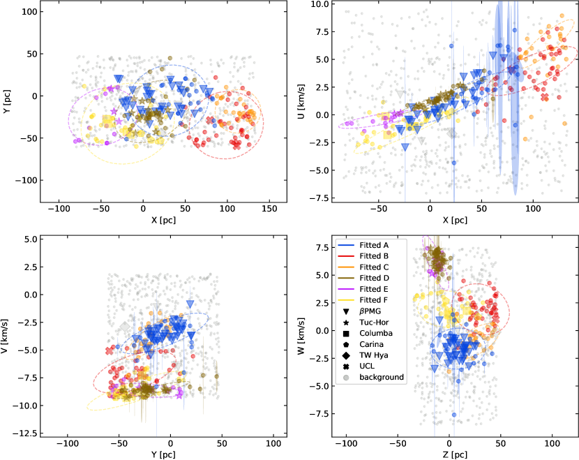
Figure 9: Results from Chronostar’s decomposition of stars identified as $\beta$PMG members by BANYAN, plus surrounding Gaia DR2 stars. Panels show current-day positions and velocities of stars in several different 2D projections. Colours indicate component assignments derived by Chronostar, while marker styles show assignments of stars to groups and associations in the BANYAN catalog; circles, labelled “Background” in the legend, are stars not identified as members of any moving group or association by BANYAN, while gray points are stars assigned to the background component by Chronostar. Filled ellipses around the current-day positions show the error distributions for the measurements; for clarity we only show error ellipses for probable members of components A and D. The dashed ellipses show the best-fit current-day distributions retrieved by Chronostar, coloured by component. Component properties derived by Chronostar are provided in Table 5, while a list of likely $\beta$PMG members is given in Table 7.

Table 5: Parameters for the $\beta$PMG and part of the Tuc-Hor moving group (see main text) derived by Chronostar’s fit to $\beta$PMG and nearby Gaia DR2 stars (Components A and D in Figure 9, respectively). We suppress here the correlations between dimensions in the covariance matrices, but the full covariance matrices can be found in the online version.

	$\beta$PMG		Partial Tuc-Hor
	Origin	Current	Origin	Current
x [pc]	$33.7^{+3.8}_{-3.4}$	$30.0^{+3.2}_{-3.1}$	$232.0^{+16.4}_{-16.5}$	$12.0^{+3.6}_{-3.6}$
y [pc]	$46.6^{+3.3}_{-3.2}$	$-5.5^{+2.8}_{-2.8}$	$155.8^{+5.3}_{-6.4}$	$-17.2^{+3.0}_{-3.0}$
z [pc]	$22.2^{+1.9}_{-1.8}$	$7.5^{+1.7}_{-1.7}$	$-20.1^{+8.7}_{-8.6}$	$-11.8^{+0.9}_{-0.8}$
u [$\,\text{km}\,\text{s}^{-1}$]	$-0.7^{+0.2}_{-0.2}$	$1.5^{+0.2}_{-0.2}$	$-7.7^{+0.4}_{-0.4}$	$1.6^{+0.1}_{-0.1}$
v [$\,\text{km}\,\text{s}^{-1}$]	$-3.4^{+0.2}_{-0.2}$	$-3.5^{+0.1}_{-0.1}$	$-2.5^{+0.5}_{-0.5}$	$-8.6^{+0.1}_{-0.1}$
w [$\,\text{km}\,\text{s}^{-1}$]	$0.2^{+0.2}_{-0.2}$	$-1.6^{+0.1}_{-0.1}$	$-6.3^{+0.2}_{-0.2}$	$6.3^{+0.1}_{-0.1}$
$\sigma_{x}$ [pc]	$12.8^{+0.9}_{-0.8}$	$24.5^{+1.5}_{-1.4}$	$4.8^{+0.4}_{-0.4}$	$23.2^{+1.7}_{-1.5}$
$\sigma_{y}$ [pc]	$12.8^{+0.9}_{-0.8}$	$21.6^{+1.2}_{-1.1}$	$4.8^{+0.4}_{-0.4}$	$19.2^{+1.4}_{-1.2}$
$\sigma_{z}$ [pc]	$12.8^{+0.9}_{-0.8}$	$13.7^{+0.9}_{-0.8}$	$4.8^{+0.4}_{-0.4}$	$5.6^{+0.4}_{-0.4}$
$\sigma_{u}[\,\text{km}\,\text{s}^{-1}]$	$1.0^{+0.1}_{-0.1}$	$1.2^{+0.1}_{-0.1}$	$0.53^{+0.04}_{-0.03}$	$0.8^{+0.1}_{-0.1}$
$\sigma_{v}[\,\text{km}\,\text{s}^{-1}]$	$1.0^{+0.1}_{-0.1}$	$0.9^{+0.1}_{-0.1}$	$0.53^{+0.04}_{-0.03}$	$0.40^{+0.03}_{-0.02}$
$\sigma_{w}[\,\text{km}\,\text{s}^{-1}]$	$1.0^{+0.1}_{-0.1}$	$1.0^{+0.1}_{-0.1}$	$0.53^{+0.04}_{-0.03}$	$0.49^{+0.03}_{-0.03}$
age [Myr]	-	$17.8^{+1.2}_{-1.2}$	-	$36.3^{+1.3}_{-1.4}$
nstars	-	$59.3$	-	$41.1$

Table 6: The BICs scored by various multi-component fits to $\beta$PMG. Each column has an entry for each unique initialisation for the given number of components. In each column the lowest BIC (in bold) is taken as the best fit for the given component count. The fit that yielded this BIC is then used to initialise multiple fits with $n+1$ components. The row denotes which component from the previous best fit Chronostar decomposes. For example, Chronostar performed two three-component fits, initialising the first by decomposing Component A of the two-component result. Chronostar initialised the second by decomposing Component B, which yielded a better BIC. Chronostar terminated with 6 components because all of the attempted 7 component fits failed to improve the BIC.

	1 comp	2 comps	3 comps	4 comps	5 comps	6 comps	7 comps
comp A	28702.90	27984.69	28311.91	27505.76	27566.69	27501.87	27479.64
comp B			27752.75	27818.54	27449.76	27489.28	27481.18
comp C				27761.06	27558.12	27449.33	27506.65
comp D					27563.82	27481.90	27494.94
comp E						27440.57	27500.21
comp F							27448.21

Figure 10: Colour-magnitude diagram of our fit to $\beta$PMG, featuring all stars in the set described by Section 4.1. Grey dots are background Gaia stars, with a clear clustering on the main sequence. The dashed orange line is an empirical fit to the main sequence. Blue markers denote $\beta$PMG members according to Chronostar. Stars that are also $\beta$PMG members according to BANYAN have circle markers, while those that are new members have triangle markers. BANYAN members that are rejected by Chronostar are shown as pink circles. The three Chronostar members that appear photometrically inconsistent are coloured red.

Table 7: Astrometry and memberships to $\beta$PMG (Comp A) as well as reference to previous work listing star as member of $\beta$PMG. Full table available in machine-readable format in online version. $\beta$PMG membership references: (1) Gagné et al. (2018b), (2) Schlieder et al. (2010), (3) Alonso-Floriano et al. (2015), (4) Moor et al. (2006), (5) Elliott et al. (2014), (6) Moór et al. (2013), (7) Torres et al. (2008), (8) Gagné et al. (2018c), (9) Zuckerman et al. (2001), (10) Malo et al. (2013), (11) Malo et al. (2014), (12) Kiss et al. (2011), (13) Elliott et al. (2016), (29) Gagné & Faherty (2018), (30) Gagné et al. (2018a), (31) Neuhäuser & Forbrich (2008). RV references: (14) Torres et al. (2006), (15) Gaia Collaboration et al. (2018), (16) Kiss et al. (2011), (17) Allers et al. (2016), (18) Shkolnik et al. (2017), (19) Torres et al. (2009), (20) Gontcharov (2006), (21) Malo et al. (2014), (22) Valenti & Fischer (2005), (23) Anderson & Francis (2012), (24) Song et al. (2003), (25) Montes et al. (2001), (26) Kharchenko et al. (2007), (27) Shkolnik et al. (2012), (28) Faherty et al. (2016).

Main	R.A.	Decl	Parallax	$\mu_{\alpha}\cos\delta$	$\mu_{\delta}$	RV	Comp. A	RV ref	Prev.
Designation	[deg]	[deg]	[mas]	[mas$\,\text{yr}^{-1}$]	[mas$\,\text{yr}^{-1}$]	[$\,\text{km}\,\text{s}^{-1}$]	Memb. Prob.		$\beta$PMG ref
HD 203	$1.709$	$-23.108$	$25.02\pm 0.06$	$96.8\pm 0.1$	$-47.12\pm 0.07$	$7\pm 4$	0.9836	20	1
RBS 38	$4.349$	$-66.753$	$27.17\pm 0.03$	$103.04\pm 0.05$	$-16.87\pm 0.05$	$10.7\pm 0.2$	0.99927	21	1
GJ 2006 A	$6.960$	$-32.552$	$28.66\pm 0.07$	$109.8\pm 0.1$	$-47.39\pm 0.07$	$8.8\pm 0.2$	0.99731	21	1
| GJ 2006 B	$6.960$	$-32.557$	$28.68\pm 0.08$	$112.2\pm 0.1$	$-44.64\pm 0.07$	$8.5\pm 0.2$		21	1
Barta 161 12	$23.808$	$-7.215$	$26.82\pm 0.09$	$97.5\pm 0.2$	$-49.09\pm 0.09$	$6.8\pm 0.8$	0.93598	21	1
G 271-110	$24.231$	$-6.794$	$41.7\pm 0.1$	$173.5\pm 0.3$	$-100.1\pm 0.2$	$12.2\pm 0.4$	0.0	27	1
HD 14082 A	$34.356$	$28.745$	$25.13\pm 0.04$	$86.92\pm 0.07$	$-74.07\pm 0.07$	$5.4\pm 0.5$	0.89691	22	1
| HD 14082 B	$34.353$	$28.741$	$25.16\pm 0.05$	$85.97\pm 0.08$	$-71.11\pm 0.08$	$4.7\pm 0.2$		15	1
AG Tri A	$36.872$	$30.973$	$24.36\pm 0.05$	$79.68\pm 0.08$	$-72.00\pm 0.07$	$4.8\pm 0.1$	0.8783	15	1
| AG Tri B	$36.867$	$30.978$	$24.45\pm 0.08$	$82.7\pm 0.1$	$-73.49\pm 0.09$	$5\pm 1$		24	1
BD+05 378	$40.358$	$5.988$	$22.50\pm 0.08$	$79.12\pm 0.10$	$-56.6\pm 0.1$	$5.7\pm 0.4$	0.0	15	1

5 Discussion

In this paper we have described the Chronostar method for kinematic age estimation and membership classification of unbound stellar associations. Chronostar models an initial association component as a 6D Gaussian with uncorrelated positions and velocities, projects this forwards in the Galactic potential and maximizes the likelihood of the component parameters by overlap with current-day stellar measurements. Multiple components are treated with an expectation maximization (EM) algorithm, and individual components have a physical, virial prior on position and velocity dispersions. This approach differs from Rizzuto et al. (2011) and BANYAN (Gagné et al., 2018c), which do not consider time evolution, and differs from LACEwING (Riedel et al., 2017) and Miret-Roig et al. (2018), which trace stellar measurements backwards through time.

The first distinguishing feature of Chronostar is how it handles kinematic fitting and membership assignment in a self-consistent way, treating the two aspects as a single problem, and iterating through their circular dependency until convergence. Other approaches (e.g. BANYAN, LACEwING) derive association parameters from pre-defined membership lists, which in effect (after potential removal of suspected interlopers) restricts the discovery of new members to the vicinity of known members. This also impedes applying constraints on the current day distributions of associations based on what is physically plausible. For example, the classical decomposition of the Scorpius Centaurus OB association into three sub-groups has minimal physical justification (Rizzuto et al., 2011), and indeed impedes kinematic ageing techniques when performed on the large-scale structure enforced by this classification (Wright & Mamajek, 2018).

The second significant difference is Chronostar’s forward modelling of an initial, compact distribution through the Galactic potential to its current-day distribution, intrinsically anchoring the various variances and covariances of all dimensions of the 6D ellipsoid to the modelled age. One obvious benefit of this approach is the provision of kinematic ages. A second and less obvious benefit is that the tight position-velocity correlations induced by the motions of stars through the Galactic potential allow us to more confidently reject interlopers that fall well within the extent of the distribution of association members in one or more dimensions (position or velocity), but do not lie on the correct position-velocity correlation. This approach is similar to the principle behind expansion ages (e.g. Torres et al. 2008, Wright & Mamajek 2018), but whereas past applications assume linear expansion, Chronostar accounts for the effects of the Galactic potential on stellar orbits. This difference is crucial in pushing to ages $\gtrsim 10-20$ Myr, because the vertical oscillation period of stars through the Galactic plane is $\approx 80$ Myr (74 Myr in our model of the Galactic potential, and $87\pm 4$ Myr using Oort constants from Bovy 2017). Position-velocity correlations rotate 90^∘ in the $Z-W$ plane over a quarter period (c.f. the discussion in Section 3.1), so the assumption of purely linear expansion begins to fail seriously after only $\approx 10-20$ Myr. A third benefit to forward modeling as done in Chronostar is that it is considerably more robust than traceback or similar methods against observational uncertainties. Typical radial velocity errors are $\approx 1$ km s^-1 (e.g., Kraus & Hillenbrand, 2008), comparable to the intrinsic velocity dispersions of associations. As a result, as one attempts to trace stars backward, the volume of possible stellar positions balloons rapidly. Attempts to sample this volume using Monte Carlo or similar techniques have thus far proven relatively unsuccessful at delivering reliable kinematic ages (e.g., Donaldson et al., 2016; Riedel et al., 2017; Miret-Roig et al., 2018). In contrast, trace-forward combined with analysis of the overlap between a proposed association and observed stars in 6D phase-space does not suffer from this explosion of possibilities, because the phase-space volume occupied by a proposed stellar distribution is conserved as one traces it forward.

6 Conclusion and Future Work

In this paper we have presented the methodology for Chronostar, a new kinematic analysis tool to identify and age unbound stars that share a common origin. The tool requires no manual calibration or pre-selection, and simultaneously and self-consistently solves the problems of assigning stars to associations and determining the properties of those associations. We test Chronostar extensively on synthetic data sets, including ones containing multiple, overlapping components and ones where the initial positions and velocities are stars are drawn directly from a hydrodynamic simulation of star formation, and show that it returns very accurate membership assignments and kinematic ages. In tests on real data, we show that Chronostar is capable of blindly recovering the $\beta$ Pictoris and Tucana-Horologium moving groups (Figure 9), with the kinematic data used to find the latter originating solely from Gaia DR2. In the future we intend to apply Chronostar to other known associations, with incorporated radial velocities from dedicated spectroscopic surveys (i.e. RAVE (Kunder et al., 2017), GALAH (Buder et al., 2018)). This should for the first time provide reliable kinematic ages. Since Chronostar has proven to be capable of blind discovery, we also intend to search the phase-space near the Sun for previously-unknown associations.

Due to the Bayesian nature of Chronostar it is also straightforward to extend it by adding extra dimensions to the parameter space for even stronger membership classification. This includes placing priors on the ages of individual stars based on spectroscopic types, and incorporating chemical tagging into the fitting mechanism. Two further possible enhancements that we intend to pursue in future work include allowing for the possibility that associations might be born with significant position-velocity correlations (as suggested for example by Tobin et al. 2009 and Offner et al. 2009), and allowing Chronostar to fit not only unbound associations but also bound open clusters that are slowly evaporating.

Appendix A Projecting a Component through Time

This appendix details our method of taking a component’s initial distribution in 6D phase-space $\mathcal{N}(\boldsymbol{\theta};\mu_{0},\boldsymbol{\Sigma}_{0})$ and, using galpy’s orbit calculations (Bovy, 2015), projecting it forward through time by its modelled age $t_{c}$ to its current-day distribution $\mathcal{N}(\boldsymbol{\theta};\mu_{c},\boldsymbol{\Sigma}_{c})$.

The technical details of the implementation used by galpy to calculate orbits are irrelevant for our method so we abstract the galpy orbit calculation as a function $\mathbf{f}$ that maps a starting point $\boldsymbol{\theta}_{0}$ in the 6D phase-space forward over an arbitrary time to a new point $\boldsymbol{\theta}_{f}$. Thus we use $\mathbf{f}$ to project $\boldsymbol{\mu}_{0}$ and $\boldsymbol{\Sigma}_{0}$ to their current-day values, $\boldsymbol{\mu}_{c}$ and $\boldsymbol{\Sigma}_{c}$. Acquiring the current-day central value is simply a matter of evolving the initial central point forward by the modelled age. In our abstracting notation this reads:

$$\boldsymbol{\mu}_{c}=\mathbf{f}(\boldsymbol{\mu}_{0},t_{c}).$$ (15)

To transform the covariance matrix $\boldsymbol{\Sigma}_{0}$ it is useful to think in terms of a coordinate transformation between two systems: the initial coordinates, and the current-day coordinates. To linear order, the covariance matrix $\boldsymbol{\Sigma}_{B}$ in the new coordinate system $B$ is given by the usual law for error propagation,

$$\boldsymbol{\Sigma}_{B}=\mathbf{J}_{A}\boldsymbol{\Sigma}_{A}\mathbf{J}_{A}^{T},$$ (16)

where $\boldsymbol{\Sigma}_{A}$ is the covariance matrix in the original coordinates $A$, and $\mathbf{J}$ is the Jacobian for the mapping between the two coordinate systems; specifically, if some function $\mathbf{g}(\mathbf{a})$ maps a point $\mathbf{a}$ in coordinate system $A$ to a corresponding point in $B$, then $\mathbf{J}_{ij}=\partial g_{i}/\partial a_{j}$.

In our case of orbit evolution, the mapping function $\mathbf{g}$ is simply $\mathbf{f}(\boldsymbol{\mu}_{0},t_{c})$, and thus the Jacobian evaluated at starting phase-space position $\boldsymbol{\mu}_{0}$ is

$$\mathbf{J}_{ij}=\frac{\partial}{\partial\theta_{0,j}}\left(f(\mu_{0},t_{c})_{i}\right)=\frac{\partial\theta_{c,i}}{\partial\theta_{0,j}},$$ (17)

where $\theta_{0,i}$ and $\theta_{c,i}$ are the $i$th components of $\boldsymbol{\mu}_{0}$ and $\boldsymbol{\mu}_{c}=\mathbf{f}(\boldsymbol{\mu}_{0},t_{c})$, respectively. That is, $\theta_{0,i}$ and $\theta_{c,i}$ are the $i$th components of the phase-space coordinates of the association’s centre at the time of its birth and at the current time, respectively. We cannot evaluate the Jacobian $\mathbf{J}$ analytically because evaluation of $\mathbf{f}$ requires numerical integration of an orbit through the Galactic potential. Instead, we evaluate the partial derivatives numerically using a second-order approximation:

$$\frac{\partial\theta_{c,i}}{\partial\theta_{0,j}}\approx\frac{f(\boldsymbol{\theta}_{0}+\boldsymbol{h},t)_{i}-f(\boldsymbol{\theta}_{0}-\boldsymbol{h},t)_{i}}{2|h|},$$ (18)

where $\boldsymbol{h}$ is a six-dimensional vector with $h_{j}=10^{-5}$ (pc or $\,\text{km}\,\text{s}^{-1}$, depending on dimension) and all other components zero.

One might worry about the numerical stability of this procedure, and this would indeed be a concern if the potential through which we were integrating the orbits were tabulated numerically, or contained significant small-scale structure. However, our potential is both analytic and very smooth, and as a result both the orbit integration and the numerical derivative returned by Equation 18 are extremely robust to changes in $\boldsymbol{h}$ as long as all components of $\boldsymbol{h}$ are much smaller than the size scale on which the potential varies, and much larger than the $\approx 10^{-8}$ error tolerance in the numerical integrator. To confirm this directly, we have experimented with varying $h$ from $10^{-1}$ to $10^{-6}$. We find that, over this range, the non-zero components of $\partial\theta_{c,i}/\partial\theta_{0,j}$ vary by $<0.01\%$ in the vast majority of cases, and by $<1\%$ in all cases.

Appendix B Exploring dependence on potential model

The choice of the potential model influences the calculated orbits and thus the resulting age fits. To explore the dependence we repeat the test described in Section 3.3.2 using two different potential models. In both cases we use the same synethetic data which we generated using the potential model MWPotential2014, but then use Chronostar to fit the stellar population using a different potential, in order to determine how sensitive our results are to uncertainties in the potential.

The two key timescales of our potential model are the vertical oscillation frequency and the epicyclic frequency. We expect the vertical oscillation period to have the greater effect on on the age fit as this is the shorter timescale by a factor of 2. Therefore in the two following tests we alter the potential by varying the scale height of the disc component. In the first test we halve the scale height, and in the second we double it. These new potentials have vertical oscillation periods scaled by 0.73 and 1.33 respectively.

Fitting the synthetic data described in Section 3.3.2 using a potential with a halved scale height continues to yield two components, with estimated ages of $6.8^{+0.2}_{-0.1}\,\text{Myr}$ and $9.9^{+0.1}_{-0.2}\,\text{Myr}$. The corresponding results for a potential with a doubled scale height are $6.8\pm 0.1\,\text{Myr}$ and $9.9\pm 0.1\,\text{Myr}$. These compare well with the true ages of 7 and 10 Myr, and with the ages determined using the correct potential. Thus despite the vertical oscillation frequency differing significantly in these two tests, and thus distorting the best fit in the $Z-W$ plane, there is sufficient constraining information in the remaining dimensions to accurately retrieve the ages. The implication of this test is that our age estimates are relatively robust to errors in any particular dimension of the potential.

References

- Allers et al. (2016) Allers K. N., Gallimore J. F., Liu M. C., Dupuy T. J., 2016, The Astrophysical Journal, 819, 133
- Alonso-Floriano et al. (2015) Alonso-Floriano F. J., Caballero J. A., Cortés-Contreras M., Solano E., Montes D., 2015, Astronomy & Astrophysics, 583, A85
- Anderson & Francis (2012) Anderson E., Francis C., 2012, Astronomy Letters, 38, 331
- Bovy (2015) Bovy J., 2015, The Astrophysical Journal Supplement Series, 216, 29
- Bovy (2017) Bovy J., 2017, Monthly Notices of the Royal Astronomical Society, 468, L63
- Buder et al. (2018) Buder S., et al., 2018, Monthly Notices of the Royal Astronomical Society
- Donaldson et al. (2016) Donaldson J. K., Weinberger A. J., Gagne J., Faherty J. K., Boss A. P., Keiser S. A., 2016, The Astrophysical Journal, 833, 95
- Ducourant et al. (2014) Ducourant C., Teixeira R., Galli P. A. B., Le Campion J. F., Krone-Martins A., Zuckerman B., Chauvin G., Song I., 2014, Astronomy and Astrophysics, 563, A121
- Elliott et al. (2014) Elliott P., Bayo A., Melo C. H. F., Torres C. a. O., Sterzik M., Quast G. R., 2014, Astronomy & Astrophysics, 568, A26
- Elliott et al. (2016) Elliott P., Bayo A., Melo C. H. F., Torres C. a. O., Sterzik M. F., Quast G. R., Montes D., Brahm R., 2016, Astronomy & Astrophysics, 590, A13
- Faherty et al. (2016) Faherty J. K., et al., 2016, The Astrophysical Journal Supplement Series, 225, 10
- Federrath (2015) Federrath C., 2015, Monthly Notices of the Royal Astronomical Society, 450, 4035
- Federrath et al. (2017) Federrath C., Krumholz M., Hopkins P. F., 2017, Journal of Physics: Conference Series, 837, 012007
- Foreman-Mackey et al. (2013) Foreman-Mackey D., Hogg D. W., Lang D., Goodman J., 2013, Publications of the Astronomical Society of the Pacific, 125, 306
- Gagné & Faherty (2018) Gagné J., Faherty J. K., 2018, The Astrophysical Journal, 862, 138
- Gagné et al. (2018a) Gagné J., Faherty J. K., Fontaine G., 2018a, Research Notes of the American Astronomical Society, 2, 9
- Gagné et al. (2018b) Gagné J., et al., 2018b, The Astrophysical Journal, 856, 23
- Gagné et al. (2018c) Gagné J., Roy-Loubier O., Faherty J. K., Doyon R., Malo L., 2018c, The Astrophysical Journal, 860, 43
- Gagné et al. (2018d) Gagné J., Faherty J. K., Mamajek E. E., 2018d, The Astrophysical Journal, 865, 136
- Gaia Collaboration et al. (2018) Gaia Collaboration et al., 2018, Astronomy and Astrophysics, 616, A11
- Gontcharov (2006) Gontcharov G. A., 2006, Astronomy Letters, 32, 759
- Johnson & Soderblom (1987) Johnson D. R. H., Soderblom D. R., 1987, The Astronomical Journal, 93, 864
- Jones et al. (2001) Jones E., Oliphant T. E., Peterson P., et al., 2001, SciPy: Open Source Scientific Tools for Python, http://www.scipy.org/
- Kharchenko et al. (2007) Kharchenko N. V., Scholz R.-D., Piskunov A. E., Röser S., Schilbach E., 2007, Astronomische Nachrichten, 328, 889
- Kiss et al. (2011) Kiss L. L., et al., 2011, Monthly Notices of the Royal Astronomical Society, 411, 117
- Kraus & Hillenbrand (2007) Kraus A. L., Hillenbrand L. A., 2007, The Astronomical Journal, 134, 2340
- Kraus & Hillenbrand (2008) Kraus A. L., Hillenbrand L. A., 2008, The Astrophysical Journal Letters, 686, L111
- Kraus et al. (2014) Kraus A. L., Shkolnik E. L., Allers K. N., Liu M. C., 2014, The Astronomical Journal, 147, 146
- Kunder et al. (2017) Kunder A., et al., 2017, The Astronomical Journal, 153, 75
- Makarov (2007) Makarov V. V., 2007, The Astrophysical Journal Supplement Series, 169, 105
- Malo et al. (2013) Malo L., Doyon R., Lafreniere D., Artigau É., Gagné J., Baron F., Riedel A., 2013, The Astrophysical Journal, 762, 88
- Malo et al. (2014) Malo L., Artigau É., Doyon R., Lafreniere D., Albert L., Gagné J., 2014, The Astrophysical Journal, 788, 81
- Mamajek & Bell (2014) Mamajek E. E., Bell C. P. M., 2014, Monthly Notices of the Royal Astronomical Society, 445, 2169
- McLachlan & Peel (2004) McLachlan G., Peel D., 2004, Finite Mixture Models. John Wiley & Sons
- Miret-Roig et al. (2018) Miret-Roig N., Antoja T., Romero-Gómez M., Figueras F., 2018, Astronomy & Astrophysics, 615, A51
- Montes et al. (2001) Montes D., López-Santiago J., Gálvez M. C., Fernández-Figueroa M. J., De Castro E., Cornide M., 2001, Monthly Notices of the Royal Astronomical Society, 328, 45
- Moor et al. (2006) Moor A., Abraham P., Derekas A., Kiss C., Kiss L. L., Apai D., Grady C., Henning T., 2006, The Astrophysical Journal, 644, 525
- Moór et al. (2013) Moór A., Szabó G. M., Kiss L. L., Kiss C., Ábrahám P., Szulágyi J., Kóspál Á., Szalai T., 2013, Monthly Notices of the Royal Astronomical Society, 435, 1376
- Neuhäuser & Forbrich (2008) Neuhäuser R., Forbrich J., 2008, in , Handbook of Star Forming Regions, Volume II. p. 735, http://adsabs.harvard.edu/abs/2008hsf2.book..735N
- Offner et al. (2009) Offner S. S. R., Hansen C. E., Krumholz M. R., 2009, The Astrophysical Journal Letters, 704, L124
- Onus et al. (2018) Onus A., Krumholz M. R., Federrath C., 2018, Monthly Notices of the Royal Astronomical Society, 479, 1702
- Ortega et al. (2002) Ortega V. G., de la Reza R., Jilinski E., Bazzanella B., 2002, The Astrophysical Journal Letters, 575, L75
- Ortega et al. (2004) Ortega V. G., de la Reza R., Jilinski E., Bazzanella B., 2004, The Astrophysical Journal, 609, 243
- Riedel et al. (2017) Riedel A. R., Blunt S. C., Lambrides E. L., Rice E. L., Cruz K. L., Faherty J. K., 2017, The Astronomical Journal, 153, 95
- Rizzuto et al. (2011) Rizzuto A. C., Ireland M. J., Robertson J. G., 2011, Monthly Notices of the Royal Astronomical Society, 416, 3108
- Rizzuto et al. (2015) Rizzuto A. C., Ireland M. J., Kraus A. L., 2015, Monthly Notices of the Royal Astronomical Society, 448, 2737
- Schlieder et al. (2010) Schlieder J. E., Lépine S., Simon M., 2010, The Astronomical Journal, 140, 119
- Schönrich et al. (2010) Schönrich R., Binney J., Dehnen W., 2010, Monthly Notices of the Royal Astronomical Society, 403, 1829
- Schwarz (1978) Schwarz G., 1978, The Annals of Statistics, 6, 461
- Scott (1992) Scott D. W., 1992, Multivariate Density Estimation: Theory, Practice, and Visualization. Wiley, Hoboken, NJ, doi:10.1002/9781118575574
- Shkolnik et al. (2012) Shkolnik E. L., Anglada-Escudé G., Liu M. C., Bowler B. P., Weinberger A. J., Boss A. P., Reid I. N., Tamura M., 2012, The Astrophysical Journal, 758, 56
- Shkolnik et al. (2017) Shkolnik E. L., Allers K. N., Kraus A. L., Liu M. C., Flagg L., 2017, The Astronomical Journal, 154, 69
- Song et al. (2003) Song I., Zuckerman B., Bessell M. S., 2003, The Astrophysical Journal, 599, 342
- Tobin et al. (2009) Tobin J. J., Hartmann L., Furesz G., Mateo M., Megeath S. T., 2009, The Astrophysical Journal, 697, 1103
- Torres et al. (2006) Torres C. A. O., Quast G. R., da Silva L., de La Reza R., Melo C. H. F., Sterzik M., 2006, Astronomy and Astrophysics, 460, 695
- Torres et al. (2008) Torres C. a. O., Quast G. R., Melo C. H. F., Sterzik M. F., 2008, Handbook of Star Forming Regions, Volume II, 5, 757
- Torres et al. (2009) Torres R. M., Loinard L., Mioduszewski A. J., Rodríguez L. F., 2009, The Astrophysical Journal, 698, 242
- Valenti & Fischer (2005) Valenti J. A., Fischer D. A., 2005, The Astrophysical Journal Supplement Series, 159, 141
- Wright & Mamajek (2018) Wright N. J., Mamajek E. E., 2018, Monthly Notices of the Royal Astronomical Society, 476, 381
- Zuckerman et al. (2001) Zuckerman B., Song I., Bessell M. S., Webb R. A., 2001, The Astrophysical Journal Letters, 562, L87