Renormalization group analysis of the hyperbolic sine-Gordon model
– Asymptotic freedom from cosh interaction –

Abstract

We present a renormalization group analysis for the hyperbolic sine-Gordon (sinh-Gordon) model in two dimensions. We derive the renormalization group equations based on the dimensional regularization method and the Wilson method. The same equations are obtained using both these methods. We have two parameters $\alpha$ and $\beta\equiv\sqrt{t}$ where $\alpha$ indicates the strength of interaction of a real salar field and $t=\beta^{2}$ is related with the normalization of the action. We show that $\alpha$ is renormalized to zero in the high-energy region, that is, the sinh-Gordon theory is an asymptotically free theory. We also show a non-renormalization property that the beta function of $t$ vanishes in two dimensions.

I Introduction

The sine-Gordon model is an important model and plays a significant role in physicscol75 ; das75 ; jos77 ; sam78 ; zam79 ; ami80 ; wie78 ; bal00 ; raj82 ; man04 ; col85 ; mar17 ; wei15 ; her07 . It is known that the sine-Gordon model is equivalent to the massive Thirring model in the weak coupling phasecol75 ; man75 ; sch77 ; fab01 . The sine-Gordon model has universality in the sense that there are many phenomena that are closely related to it. The two-dimensional sine-Gordon model is mapped to the Coulomb gas model with logarithmic Coulomb interactionsam78 ; jos76 ; zin89 .

The hyperbolic sine-Gordon model (sinh-Gordon model) is similar to the sine-Gordon model, where the cosine potential is replaced by the hyperbolic cosine one. The sinh-Gordon model has been studied as a field theory modeling86 ; kou93 ; fri93 ; waz05 ; byt06 ; hoe07 ; tes08 . It appears that the sinh-Godron model is similar to the $\phi^{4}$ model when we expand $\cosh\phi$ in terms of $\phi$. In fact, both models have a kink solution as a classical solution. There is, however, the significant difference between these models that the $\phi^{4}$ model is renormalized in four dimensions while the sinh-Gordon model is renormalizable in two dimensions.

The Lagrangian of the sine-Gordon model is given as

$$\mathcal{L}=\frac{1}{2t}(\partial_{\mu}\phi)^{2}+\frac{\alpha}{t}\cos\phi,$$ (1)

for a real scalar field $\phi$. This is written as

$$\mathcal{L}=\frac{1}{2}(\partial_{\mu}\phi)^{2}+g\cos(\beta\phi),$$ (2)

where $\beta=\sqrt{t}$ and $g=\alpha/t$ with the transformation $\phi\rightarrow\beta\phi$. The sinh-Gordon model is obtained by performing the transformation in Eq. (2):

$$\beta \rightarrow i\beta,$$ (3)

$$g \rightarrow -g.$$ (4)

In this paper we investigate the sinh-Gordon model by using the renormalization group theory. We use the dimensional regularization methodtho72 ; gro76 as well as the Wilson renormalization group methodwil75 ; kog79 . The beta functions are derived using these methods and show that the coupling constant for the hyperbolic cosine potential decreases as the energy scale increases. Namely, the model shows an asymptotic freedom.

The paper is organized as follows. In Sect. 2, we present the model that we consider in this paper. In Sect. 3, we derive renormalization group equations on the basis of the dimensional regularization method. In Sect. 4, we examine the renormalization procedure based on the Wilson method, and in Sect. 5 we investigate the scaling property. In Sect. 6 we consider the generalized model with high-frequency modes and examine their effect on scaling property. A summary is given in the final section.

II Sinh-Gordon model

We consider the Lagrangian density for a real scalar field $\phi$:

$$\mathcal{L}=\frac{1}{2t_{0}}(\partial_{\mu}\phi_{B})^{2}-\frac{\alpha_{0}}{t_{0}}\cosh(\phi_{B}),$$ (5)

where $t_{0}$ and $\alpha_{0}$ are bare coupling constants, and $\phi_{B}$ is a bare real scalar field. The second term is the potential energy given by the hyperbolic cosine function $\cosh\phi=(e^{\phi}+e^{-\phi})/2$. $t$ and $\alpha$ denote the renormalized coupling constants. They are related to bare quantities through the relations given as

$$t_{0} = t\mu^{2-d}Z_{t},$$ (6)

$$\alpha_{0} = \alpha\mu^{2}Z_{\alpha},$$ (7)

where $Z_{t}$ and $Z_{\alpha}$ are renormalization constants. We introduced the energy scale $\mu$ so that $t$ and $\alpha$ are dimensionless constants. We adopt that $t$ and $\alpha$ are positive: $t>0$ and $\alpha>0$. The renormalized field $\phi_{R}$ is defined by

$$\phi_{B}=\sqrt{Z_{\phi}}\phi_{R},$$ (8)

where we introduced the renormalization constant $Z_{\phi}$ for the field $\phi$. Then, the Lagrangian with renormalized quantities is

$$\mathcal{L}=\frac{\mu^{d-2}Z_{\phi}}{2tZ_{t}}(\partial_{\mu}\phi)^{2}-\frac{\mu^{d}\alpha Z_{\alpha}}{tZ_{t}}\cosh(\sqrt{Z_{\phi}}\phi),$$ (9)

where $\phi$ indicates the renormalized field $\phi_{R}$.

We consider the Euclidean action for convenience. The action for the sinh-Gordon model in $d$ dimensions reads

$$S=\int d^{d}x\Big{[}\frac{\mu^{d-2}Z_{\phi}}{2tZ_{t}}(\partial_{\mu}\phi)^{2}+\frac{\mu^{d}\alpha Z_{\alpha}}{tZ_{t}}\cosh(\sqrt{Z_{\phi}}\phi)\Big{]}.$$ (10)

III Renormalization group equations

III.1 Renormalization of $\alpha$

We consider tadpole diagrams to take account of the renormalization of $\alpha$ up to the lowest order of $\alpha$ (Fig. 1)ami80 ; yan16 ; yan17 ; yan18 . Using the expansion $\cosh\phi=1+(1/2)\phi^{2}+(1/4!)\phi^{4}+\cdots$, the hyperbolic cosine function is renormalized in a similar way to the sine-Gordon model, as

$$\cosh(\sqrt{Z_{\phi}}\phi) \rightarrow \left(1+\frac{1}{2}Z_{\phi}\langle\phi^{2}\rangle+\cdots\right)\cosh(\sqrt{Z_{\phi}}\phi)$$ (11)

$$= \exp\left(\frac{1}{2}Z_{\phi}\langle\phi^{2}\rangle\right)\cosh(\sqrt{Z_{\phi}}\phi).$$

The expectation value $\langle\phi^{2}\rangle$ is evaluated as

$$Z_{\phi}\langle\phi^{2}\rangle = t\mu^{2-d}Z_{t}\int\frac{d^{d}k}{(2\pi)^{d}}\frac{1}{k^{2}+m_{0}^{2}}$$ (12)

$$= -\frac{1}{\epsilon}t\frac{\Omega_{d}}{(2\pi)^{d}},$$

where we put

$$d=2+\epsilon.$$ (13)

$m_{0}$ was introduced to avoid the infrared divergence and $\Omega_{d}$ is the solid angle in $d$ dimensions. In general, the divergent terms such as $t^{n}/\epsilon^{n}$ for $n\geq 2$ will be cancelled in a renormalization procedure. We choose $Z_{\alpha}$ to cancel the divergence as

$$Z_{\alpha}=1+\frac{1}{2\epsilon}\frac{t}{2\pi}+\frac{1}{8\epsilon^{2}}\left(\frac{t}{2\pi}\right)^{2}+\cdots=\exp\left(\frac{t}{4\pi\epsilon}\right),$$ (14)

near two dimensions. We have $\mu\partial\alpha_{0}/\partial\mu=0$, since the bare coupling constant $\alpha_{0}$ is independent of the energy scale $\mu$. This leads to

$$\beta(\alpha)\equiv\mu\frac{\partial\alpha}{\partial\mu}=-2\alpha-\alpha\mu\frac{\partial\ln Z_{\alpha}}{\partial\mu}.$$ (15)

Similarly we have

$$\beta(t)\equiv\mu\frac{\partial t}{\partial\mu}=(d-2)t-t\mu\frac{\partial\ln Z_{t}}{\partial\mu}.$$ (16)

Because $Z_{t}=1$ up to the lowest order of $\alpha$, we obtain up to the first order of $t$,

$$\mu\frac{\partial\ln Z_{\alpha}}{\partial\mu}=\frac{1}{4\pi\epsilon}\mu\frac{\partial t}{\partial\mu}=\mu\frac{1}{Z_{\alpha}}\frac{\partial Z_{\alpha}}{\partial\mu}=\frac{t}{4\pi}.$$ (17)

This results in

$$\beta(\alpha)=-2\alpha-\frac{1}{4\pi}\alpha t=-2\alpha\left(1+\frac{1}{8\pi}t\right).$$ (18)

This expression holds near two dimensions. It then appears that $\beta(\alpha)$ has zero only at $\alpha=0$ since $t>0$, which is shown in Fig. 2. $\beta(\alpha)$ is always negative indicating that the asymptotic freedom is a feature of sinh-Gordon model.

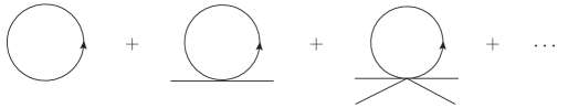
Figure 1: Tadpole diagrams for the renormalization of $\alpha$.

Figure 2: The beta function $\beta(\alpha)$ as a function of $\alpha$. The arrow indicates the flow as $\mu\rightarrow\infty$.

III.2 Renormalization of $t$

Let us examine the renormalization effect on the coupling constant $t$. We consider the correction to the kinetic part of the action. The correction to the action in the second order of $\alpha$ is given by

$$S^{(2)} = -\frac{1}{2}\left(\frac{\mu^{d}}{tZ_{t}}\right)^{2}\left(\alpha Z_{\alpha}\right)^{2}\int d^{d}xd^{d}x^{\prime}\cosh\left(\sqrt{Z_{\phi}}\phi(x)\right)$$ (19)

$$\times\cosh\left(\sqrt{Z_{\phi}}\phi(x^{\prime})\right)$$

$$= -\frac{1}{4}\left(\frac{\mu^{d}}{tZ_{t}}\right)^{2}\left(\alpha Z_{\alpha}\right)^{2}\int d^{d}xd^{d}x^{\prime}\Big{[}$$

$$\cosh\left(\sqrt{Z_{\phi}}(\phi(x)+\phi(x^{\prime}))\right)$$

$$+\cosh\left(\sqrt{Z_{\phi}}(\phi(x)-\phi(x^{\prime}))\right)\Big{]}.$$

The term with $\cosh\left(\sqrt{Z_{\phi}}(\phi(x)+\phi(x^{\prime}))\right)$ gives an effective potential with high-frequency mode, which is not examined in this section. The second term $\cosh\left(\sqrt{Z_{\phi}}(\phi(x)-\phi(x^{\prime}))\right)$ will give a correction to the kinetic term, thus to the renormalization of $t$.

Based on the tadpole approximation where we consider diagrams shown in Fig. 1, $\cosh\left(\sqrt{Z_{\phi}}(\phi(x)-\phi(x^{\prime}))\right)$ is renormalized as

$$\cosh\left(\sqrt{Z_{\phi}}(\phi(x)-\phi(x^{\prime}))\right) \rightarrow \exp\left(\frac{1}{2}Z_{\phi}\langle(\phi(x)-\phi(x^{\prime}))^{2}\rangle\right)$$

$$\times \cosh\left(\sqrt{Z_{\phi}}(\phi(x)-\phi(x^{\prime}))\right).$$

Then we have

$$S^{(2)} \simeq -\frac{1}{4}\left(\frac{\mu^{d}}{tZ_{t}}\right)^{2}\left(\alpha Z_{\alpha}\right)^{2}\int d^{d}xd^{d}x^{\prime}\Big{[}$$ (21)

$$\times \exp\left(\frac{1}{2}Z_{\phi}\langle\phi(x)^{2}+\phi(x^{\prime})^{2}\rangle-Z_{\phi}\langle\phi(x)\phi(x^{\prime})\rangle\right)$$

$$\times \cosh\left(\sqrt{Z_{\phi}}(\phi(x)-\phi(x^{\prime}))\right)\Big{]}.$$

The correlation function $\langle\phi(x)\phi(x^{\prime})\rangle$ is written as

$$\langle\phi(x)\phi(x^{\prime})\rangle=\frac{t\mu^{2-d}Z_{t}}{Z_{\phi}}\frac{\Omega_{d}}{(2\pi)^{d}}K_{0}(m_{0}|x-x^{\prime}|),$$ (22)

where $K_{0}(z)$ is the zeroth modified Bessel function. $K_{0}(z)$ divergently increases as $z$ approaches zero. Then, $\exp(-Z_{\phi}\langle\phi(x)\phi(x^{\prime})\rangle)$ becomes very small when $|x-x^{\prime}|$ is small. A dominant contribution comes from the region where $|x-x^{\prime}|$ is large. This indicates that $S^{(2)}$ gives no contribution to the renormalization of the kinetic term since we cannot expand $S^{(2)}$ with respect to ${\bf r}$ where ${\bf r}=x^{\prime}-x$. Thus, there is no renormalization of $t$ up to the second order of $\alpha$. This is in contrast to the result for the sine-Gordon model where $\exp(-Z_{\phi}\langle\phi(x)\phi(x^{\prime})\rangle)$ becomes very large for $x-x^{\prime}\sim 0$. The beta function for $t$ is now given as

$$\beta(t)=(d-2)t.$$ (23)

IV Wilson renormalization group method

Let us examine the renormalization group theory for the sinh-Gordon model based on the Wilson renormalization group method. In Wilson’s method, we start from the action

$$S=\int d^{2}x\Big{[}\frac{1}{2}(\partial_{\mu}\phi(x))^{2}+g\cosh(\beta\phi(x))\Big{]},$$ (24)

with the cutoff $\Lambda$ in the momentum space. We consider corrections to the action when we reduce the cutoff from $\Lambda$ to $\Lambda-d\Lambda$. The field $\phi(x)$ is divided into two terms $\phi(x)=\phi_{1}(x)+\phi_{2}(x)$ where

$$\phi_{1}(x) = \int_{0\leq|{\bf k}|\leq\Lambda-d\Lambda}\frac{d^{2}k}{(2\pi)^{2}}e^{i{\bf k}\cdot{\bf x}}\phi({\bf k}),$$

$$\phi_{2}(x) = \int_{\Lambda-d\Lambda\leq|{\bf k}|\leq\Lambda}\frac{d^{2}k}{(2\pi)^{2}}e^{i{\bf k}\cdot{\bf x}}\phi({\bf k}).$$ (25)

The action is written as

$$S = \int d^{2}x\left[\frac{1}{2}(\partial_{\mu}\phi_{1})^{2}+\frac{1}{2}(\partial_{\mu}\phi_{2})^{2}+g\cosh(\beta(\phi_{1}+\phi_{2}))\right]$$ (26)

$$= S_{0}(\phi_{1})+S_{0}(\phi_{2})+S_{1}(\phi_{1},\phi_{2}).$$

The last term $S_{1}$ is regarded as a perturbation. Since the potential $\cosh\beta(\phi_{1}+\phi_{2})$ is approximated as

$$\cosh\beta(\phi_{1}+\phi_{2}) = \cosh(\beta\phi_{1})\left(1+\frac{1}{2}\beta^{2}\phi_{2}^{2}+\cdots\right)$$ (27)

$$+\sinh\beta(\phi_{1})(\beta\phi_{2}+\cdots),$$

the correction to the action $S_{0}(\phi_{1})$ in the lowest order is given by

$$S^{(1)} = \langle S_{1}\rangle=g\int d^{2}x\langle\cosh(\beta(\phi_{1}+\phi_{2}))\rangle$$ (28)

$$\simeq g\int d^{2}x\exp\left(\frac{\beta^{2}}{2}\langle\phi_{2}^{2}\rangle\right)\cosh(\beta\phi_{1})$$

$$\simeq g\left(1+\frac{\beta^{2}}{4\pi}\frac{d\Lambda}{\Lambda}\right)\int d^{2}x\cosh(\beta\phi_{1}),$$

where $\langle\cdots\rangle$ indicates the expectation value with respect to the action $S_{0}(\phi_{2})$:

$$\langle Q\rangle=\frac{1}{Z_{2}}\int d\phi_{2}Qe^{-S_{0}(\phi_{2})},$$ (29)

with $Z_{2}=\int d\phi_{2}e^{-S_{0}(\phi_{2})}$. $\langle\phi_{2}^{2}\rangle$ reads $\langle\phi_{2}(x)\phi_{2}(x^{\prime})\rangle$ for $x^{\prime}=x$ where the correlation function in this formulation is

$$\langle\phi_{2}(x)\phi_{2}(x^{\prime})\rangle = \int_{\Lambda-d\Lambda\leq|{\bf k}|\leq\Lambda}\frac{d^{2}k}{(2\pi)^{2}}e^{i{\bf k}\cdot(x-x^{\prime})}\langle\phi_{2}({\bf k})\phi_{2}(-{\bf k})\rangle$$ (30)

$$= \frac{1}{2\pi}J_{0}(\Lambda|x-x^{\prime}|)\frac{d\Lambda}{\Lambda},$$

where $\langle\phi_{2}({\bf k})\phi_{2}(-{\bf k})\rangle=1/k^{2}$ and $J_{0}(z)$ is the zeroth Bessel function.

The correction to $S_{0}(\phi_{1})$ in the second order of $\alpha$ is given by

$$S^{(2)} = -\frac{1}{2}g^{2}\int d^{2}xd^{2}x^{\prime}\Big{[}$$ (31)

$$\langle\cosh(\beta(\phi_{1}(x)+\phi_{2}(x)))\cosh(\beta(\phi_{1}(x^{\prime})+\phi_{2}(x^{\prime})))\rangle$$

$$-\langle\cosh(\beta(\phi_{1}(x)+\phi_{2}(x)))\rangle\langle\cosh(\beta(\phi_{1}(x^{\prime})+\phi_{2}(x^{\prime})))\rangle\Big{]}$$

$$\simeq -\frac{1}{4}g^{2}\int d^{2}xd^{2}x^{\prime}\exp\left(\beta^{2}\langle\phi_{2}(x)^{2}\rangle\right)\Big{[}$$

$$\big{[}\exp\left(\beta^{2}\langle\phi_{2}(x)\phi_{2}(x^{\prime})\rangle\right)-1\big{]}\cosh(\beta(\phi_{1}(x)+\phi_{1}(x^{\prime})))$$

$$+\big{[}\exp\left(-\beta^{2}\langle\phi_{2}(x)\phi_{2}(x^{\prime})\rangle\right)-1\big{]}$$

$$\times\cosh(\beta(\phi_{1}(x)-\phi_{1}(x^{\prime})))\Big{]}.$$

The first term with $\cosh(\beta(\phi_{1}(x)+\phi_{1}(x^{\prime})))$ gives a potential of the form $\cosh(2\phi_{1})$ which we neglect in this section. $\big{[}\exp\left(-\beta^{2}\langle\phi_{2}(x)\phi_{2}(x^{\prime})\rangle\right)-1\big{]}$ in the second term becomes small as $|x-x^{\prime}|$ decreases. Hence there is also no renormalization effect for the coupling constant $t$ up to the order of $\alpha^{2}$ in this formulation. Then, the effective action for the field $\phi_{1}$ with the cutoff $\Lambda-d\Lambda$ is

$$S_{\Lambda-d\Lambda} = \int d^{2}x\left[\frac{1}{2}(\partial_{\mu}\phi_{1})^{2}+g\left(1+\frac{\beta^{2}}{4\pi}\frac{d\Lambda}{\Lambda}\right)\cosh(\beta\phi_{1})\right].$$

We perform the scale transformation to let the cutoff be $\Lambda$:

$$x^{\prime} = e^{-d\ell}x,$$ (33)

$${\bf k}^{\prime} = e^{d\ell}{\bf k},$$ (34)

$$\phi_{1}({\bf k}) = \zeta\tilde{\phi}_{1}({\bf k}),$$ (35)

where $d\ell=d\Lambda/\Lambda$. We have

$$\phi_{1}(x) = \zeta e^{-2d\ell}\int_{0\leq|{\bf k}^{\prime}|\leq\Lambda}\frac{d^{2}k^{\prime}}{(2\pi)^{2}}e^{i{\bf k}^{\prime}\cdot x^{\prime}}\tilde{\phi}_{1}({\bf k}^{\prime})$$ (36)

$$= \zeta e^{-2d\ell}\tilde{\phi}_{1}(x^{\prime}).$$

The effective action reads

$$S_{\Lambda-d\Lambda} = \int d^{2}x^{\prime}\Big{[}\zeta^{2}e^{-4d\ell}\frac{1}{2}(\partial_{\mu}\tilde{\phi}_{1}(x^{\prime}))^{2}$$ (37)

$$+e^{2d\ell}g\left(1+\beta^{2}\frac{1}{4\pi}\frac{d\Lambda}{\Lambda}\right)\cosh(\beta\zeta e^{-2d\ell}\tilde{\phi}_{1}(x^{\prime}))\Big{]}$$

$$= \int d^{2}x^{\prime}\Big{[}\frac{1}{2}(\partial_{\mu}\tilde{\phi}_{1}(x^{\prime}))^{2}+g\left(1+2\frac{d\Lambda}{\Lambda}+\beta^{2}\frac{1}{4\pi}\frac{d\Lambda}{\Lambda}\right)$$

$$\times\cosh(\beta\tilde{\phi}_{1}(x^{\prime})\Big{]},$$

where we set $\zeta=e^{2d\ell}$. This indicates that $t$ is not renormalized and $g$ is renormalized to $g+dg$:

$$\Lambda\frac{dg}{d\Lambda}=2g+\frac{1}{4\pi}\beta^{2}g.$$ (38)

The equation for $\alpha$ reads

$$\Lambda\frac{d\alpha}{d\Lambda}=2\alpha+\frac{1}{4\pi}t\alpha.$$ (39)

Hence, we obtained the same equation as in the previous section and the effective $\alpha$ increases as the cutoff $\Lambda$ decreases to the low-energy region. Because we examined the derivative in the descent direction for $\Lambda\rightarrow\Lambda-d\Lambda$, the above equation has opposite sign to the equation in Eq. (18). Since $d\Lambda$ is related to $d\mu$ as $d\ln\Lambda=-d\ln\mu$, we have the same equation. Since the beta functions in the dimensional regularization method were obtained by fixing bare quantities, we used a partial derivative expression in Sect. 3.

V Renormalization group flow

The renormalization group equations in the lowest order of $\alpha$ and $t$ are

$$\mu\frac{\partial\alpha}{\partial\mu} = -2\alpha\left(1+\frac{1}{8\pi}t\right),$$

$$\mu\frac{\partial t}{\partial\mu} = (d-2)t.$$ (40)

In two dimensions ($d=2$), we have $t=t_{0}=$ constant and

$$\alpha=\alpha_{0}\left(\frac{\mu}{\mu_{0}}\right)^{-(2+t_{0}/4\pi)},$$ (41)

where we adopt that $\alpha=\alpha_{0}$ at $\mu=\mu_{0}$. The flow as $\mu\rightarrow\infty$ is shown in Fig. 3. $t$ remains constant, and $\alpha$ decreases and approaches zero.

For $d$ near 2, the solution is given by

$$t=t_{0}\left(\frac{\mu}{\mu_{0}}\right)^{d-2},$$ (42)

$$\alpha=\alpha_{0}\left(\frac{\mu}{\mu_{0}}\right)^{-2}\exp\left[-\frac{t_{0}}{4\pi}\frac{1}{d-2}\left(\left(\frac{\mu}{\mu_{0}}\right)^{d-2}-1\right)\right],$$ (43)

where $t_{0}$ and $\alpha_{0}$ are initial values of $t$ and $\alpha$. In the limit $d\rightarrow 2$, this set of solutions reduces to that for $d=2$. The renormalization group flow is shown in Fig. 4 for general $d$. In the high-energy region the effective $\alpha$ becomes vanishingly small, and instead in the low-energy region $\alpha$ becomes very large and will dominate the low-energy property. The function in Eq. (43) is important in the theory of the sinh-Gordon model. In a variational theorying86 , the expectation value of the potential energy is expressed with this function.

Figure 3: The renormalization group flow in two dimensions $d=2$ where the arrow indicates the flow as $\mu\rightarrow\infty$.

Figure 4: The renormalization group flow starting from $t=t_{0}$ and $\alpha=\alpha_{0}$ for $d>2$, $d=2$ and $d<2$, respectively, where the arrow indicates the flow as $\mu\rightarrow\infty$.

VI Renormalization of high-frequency modes

In the renormalization procedure in the previous section a high-frequency mode such as $\cosh(2\phi)$ appears that we have neglected so far. We examine the renormalization of high-frequency terms in this section. Let us consider the action:

$$S = \int d^{2}x\left[\frac{1}{2}(\partial_{\mu}\phi)^{2}+\sum_{n=1}g_{n}\cosh(n\beta\phi)\right]$$ (44)

$$= \int d^{2}x\Big{[}\frac{1}{2}(\partial_{\mu}\phi_{1})^{2}+\frac{1}{2}(\partial_{\mu}\phi_{2})^{2}$$

$$+\sum_{n=1}g_{n}\cosh(n\beta(\phi_{1}+\phi_{2}))\Big{]}$$

$$= S_{0}(\phi_{1})+S_{0}(\phi_{2})+S_{1}(\phi_{1},\phi_{2}),$$

where $\phi_{1}$ and $\phi_{2}$ were defined in Sect. 4. $g_{n}\equiv\alpha_{n}/t$ ($n=1,2,...$) are the coupling constants and $\beta=\sqrt{t}$. The lowest-order correction in the Wilson method is

$$S^{(1)} = \sum_{n}g_{n}\exp\left(n^{2}\frac{\beta^{2}}{2}\langle\phi_{2}^{2}\rangle\right)\int d^{2}x\cosh(n\beta\phi_{1}(x))$$

$$= \sum_{n}g_{n}\exp\left(n^{2}\frac{\beta^{2}}{4\pi}\frac{d\Lambda}{\Lambda}\right)\int d^{2}x\cosh(n\beta\phi_{1}(x)).$$

The second-order correction is given as

$$S^{(2)} = -\frac{1}{4}\sum_{nm}g_{n}g_{m}\exp\left((n^{2}+m^{2})\frac{\beta^{2}}{4\pi}\frac{d\Lambda}{\Lambda}\right)$$

$$\times\int d^{2}xd^{2}x^{\prime}\left(\exp\left(nm\beta^{2}\langle\phi_{2}(x)\phi_{2}(x^{\prime})\rangle\right)-1\right)$$

$$\times\cosh(n\beta\phi_{1}(x)+m\beta\phi_{1}(x^{\prime}))$$

$$\simeq -\frac{1}{4}\sum_{nm}nmg_{n}g_{m}\int d^{2}r\frac{\beta^{2}}{2\pi}J_{0}(\Lambda r)\frac{d\Lambda}{\Lambda}$$

$$\times\int d^{2}x\cosh((n+m)\beta\phi_{1}(x))$$

$$= -\frac{C_{\Lambda}}{4}\beta^{2}\sum_{nm}nmg_{n}g_{m}\frac{d\Lambda}{\Lambda}\int d^{2}x\cosh((n+m)\beta\phi_{1}(x)),$$

where $C_{\Lambda}$ is a constant:

$$C_{\Lambda}=\int d^{2}r\frac{1}{2\pi}J_{0}(\Lambda r).$$ (47)

Then, the effective action is

$$S_{\Lambda-d\Lambda} = \int d^{2}x\Big{[}\frac{1}{2}(\partial_{\mu}\phi_{1})^{2}+\sum_{n=1}g_{n}\left(1+\frac{n^{2}\beta^{2}}{4\pi}\frac{d\Lambda}{\Lambda}\right)\cosh(n\beta\phi_{1})$$

$$- \frac{C_{\Lambda}}{4}\beta^{2}\sum_{nm,1\leq m\leq n-1}g_{n-m}g_{m}(n-m)m\frac{d\Lambda}{\Lambda}\cosh(n\beta\phi_{1})\Big{]}.$$

After the scaling transformation $x\rightarrow x^{\prime}=e^{-d\ell}x$, this action results in the scaling equations

$$\Lambda\frac{dg_{n}}{d\Lambda} = \left(2+n^{2}\frac{\beta^{2}}{4\pi}\right)g_{n}-\frac{C_{\Lambda}}{4}\beta^{2}\sum_{1\leq m\leq n-1}m(n-m)g_{n-m}g_{m},$$

$$\Lambda\frac{d\beta}{d\Lambda}=0.$$ (50)

Since $g_{n}=\alpha_{n}/t$, we have

$$\Lambda\frac{d\alpha_{n}}{d\Lambda}=\left(2+n^{2}\frac{t}{4\pi}\right)\alpha_{n}-\frac{C_{\Lambda}}{4}\sum_{1\leq m\leq n-1}m(n-m)\alpha_{n-m}\alpha_{m}.$$ (51)

For small $n$ ($n=1,2,...$), the equations for $\alpha_{n}$ are

$$\Lambda\frac{d\alpha_{1}}{d\Lambda} = \left(2+\frac{t}{4\pi}\right)\alpha_{1},$$ (52)

$$\Lambda\frac{d\alpha_{2}}{d\Lambda} = \left(2+\frac{t}{\pi}\right)\alpha_{2}-\frac{C_{\Lambda}}{4}\alpha_{1}^{2},$$ (53)

$$\Lambda\frac{d\alpha_{3}}{d\Lambda} = \left(2+\frac{9t}{4\pi}\right)\alpha_{3}-C_{\Lambda}\alpha_{1}\alpha_{2}.$$ (54)

$\alpha_{1}$ obviously decreases to zero in the high-energy region. Thus, $\alpha_{2}$ and $\alpha_{3}$ also decreases as the energy scale increase. Hence the sinh-Gordon theory with high-frequency modes remains an asymptotically free theory.

VII Summary

We have presented a renormalization group analysis of the sinh-Gordon model. The analysis is based on the dimensional regularization method and also the Wilson renormalization group method. A set of beta functions were derived and its scaling property was discussed. In contrast to the sine-Gordon model, the sinh-Gordon model exhibits an asymptotic freedom with vanishing $\alpha$ in the limit $\mu\rightarrow\infty$ in two dimensions ($d=2$). Up to the second order of $\alpha$, the coupling constant $t$ is not renormalized in two dimensions. In Ref.ing86 , the ground-state energy was estimated by using a variational wave function. The same function as in Eq. (43) appears in the evaluation of the potential energy and plays an important role. This indicates that the two results are consistent. We have also examined the generalized model with interactions $\alpha_{n}\cosh(n\beta\phi)$ ($n=1,2,...$). It was shown based on the Wilson method that the equation for $\alpha_{1}$ remains the same and that the generalized sinh-Gordon theory is an asymptotically free theory. We obtain the same renormalization group equations by employing the dimensional regularization method, where the coefficients for higher-order terms are slightly modified.

The sinh-Gordon model belongs to a universality class showing asymptotic freedom. The nonlinear sigma model and non-Abelian Yang-Mills theory also belong in this class. Thus the sinh-Gordon model is an interesting model and may be applied to various phenomena in the future. In the infrared region, the parameter $\alpha$ increases and dominates the property of the system. The physical property is determined by the potential energy $\cosh\phi$. In this region, $\phi$ may be small since the kinetic term is negligibly small. Then, $\cosh\phi$ can be expanded by $\phi$ to investigate the low-energy property. The effective action is given by a $\phi^{4}$ theory:

$$S_{low}=\int d^{2}x\left[\frac{1}{2}(\partial_{\mu}\phi)^{2}+\frac{\alpha}{2}\phi^{2}+\frac{1}{4!}t\alpha\phi^{4}\right],$$ (55)

where we did the scale transformation $\phi\rightarrow\sqrt{t}\phi$.

VIII Acknowledgment

This work was supported by Grant-in-Aid from the Ministry of Education, Culture, Sports, Science and Technology (MEXT) of Japan (no. 17K05559).

References

• (1) S. Coleman, Phys. Rev. D11, 2088 (1975).
• (2) R. F. Dashen, B. Hasslacher and A. Neveu, Phys. Rev. D11, 3424 (1975).
• (3) J. V. Jose, I. P. Kadanoff, S. Kirkpatrick and D. R. Nelson, Phys. Rev. B16, 1217 (1977).
• (4) S. Samuel, Phys. Rev. D18, 1916 (1978).
• (5) A. B. Zamolodchikov and Al. B. Zamolodchikov, Ann. Phys. 120, 253 (1979).
• (6) D. J. Amit, Y. Y. Goldschmidt and S. Grinstein, J. Phys. A: Math. Gen. 13, 585 (1980).
• (7) P. B. Wiegmann, J. Phys. C11, 1583 (1978).
• (8) J. Balog and A. Hegedus, J. Phys. A33, 6543 (2000).
• (9) R. Rajaraman, Solitons and Instantons (North-Holland, Amsterdam, 1982).
• (10) N. S. Manton and P. Sutcliffe, Topological Solitons (Cambridge University Press, Cambridge, 2004).
• (11) S. Coleman, Aspects of Symmetry (Cambridge University Press, Cambridge, 1985).
• (12) E. C. Marino, Quantum Field Theory Approach to Condensed Matter Physics (Cambridge University Press, Cambridge, 2017).
• (13) E. Weinberg, Classical Solutions in Quantum Field Theory (Cambridge University Press, Cambridge, 2015).
• (14) I. Herbut, A Modern Approach to Critical Phenomena (Cambridge University Press, Cambridge, 2007).
• (15) S. Mandelstam, Phys. Rev. D11, 3026 (1975).
• (16) B. Schroer and T. Truong, Phys. Rev. D15, 1684 (1977).
• (17) M. Faber and A. N. Ivanov, Eur. Phys. J. C20, 723 (2001).
• (18) J. Jose, Phys. Rev. D14, 2826 (1976).
• (19) J. Zinn-Justin, Quantum Field Theory and Critical Phenomena (Oxford University Press, Oxford, 1989).
• (20) R. Ingermanson, Nucl. Phys. B266, 620 (1986).
• (21) A. Koubek and G. Mussaodo, Phys. Lett. B311, 193 (1993).
• (22) A. Fring, G. Mussardo and P. Simonetti, Nucl. Phys. B393, 413 (1993).
• (23) A.-M. Wazwaz, Appl. Math. Comp. 167, 1196 (2005).
• (24) A. G. Bytsko and J. Teschner, J. Phys. A39, 1927(2006).
• (25) C. Hoenselaers, Int. J. Theor. Phys. 46, 1096 (2007).
• (26) J. Teschner, Nucl. Phys. B799, 403 (2008).
• (27) G. ’t Hooft and M. Veltman, Nucl. Phys. B44, 189 (1972).
• (28) D. Gross, Applications of the renormalization group to high-energy physics, in Methods in Field Theory Les Houches Lecture Notes, eds. R. Balian and J. Zinn-Justin (North-Holland, Amsterdam, 1976).
• (29) K. G. Wilson, Rev. Mod. Phys. 47, 773 (1975).
• (30) J. B. Kogut, Rev. Mod. Phys. 51, 659 (1979).
• (31) T. Yanagisawa, Europhys. Lett. 113, 41001 (2016).
• (32) T. Yanagisawa, Renormalization group theory of effective field theory models in low dimensions, in Recent Studies in Perturbation Theory, ed. D. I. Uzunov (InTechOpen, London, 2017) (arXiv: 1804.02845).
• (33) T. Yanagisawa, Adv. Math. Phys. 2018, 9238280 (2018).