Dual-polarisation Non-linear Frequency-division Multiplexed Transmission with $b$-Modulation

Abstract

There has been much interest in the non-linear frequency-division multiplexing (NFDM) transmission scheme in the optical fibre communication system. Up to date, most of the demonstrated NFDM schemes have employed only single polarisation for data transmission. Employing both polarisations can potentially double the data rate of NFDM systems. We investigate in simulation a dual-polarisation NFDM transmission with data modulation on the $b$-coefficient. First, a transformation that facilitates the dual-polarisation $b$-modulation was built upon an existing transformation in [1]. Second, the $q_{c}$- and $b$-modulation for dual-polarisation were compared in terms of Q-factor, spectral efficiency (SE), and correlation of sub-carriers. The correlation is quantified via information theoretic metrics, joint and individual entropy. The polarisation-multiplexed $b$-modulation system shows 1 dB Q-factor improvement over $q_{c}$-modulation system due to a weaker correlation of sub-carriers and less effective noise. Finally, the $b$-modulation system was optimised for high data rate, achieving a record net data rate of 400 Gbps (SE of 7.2 bit/s/Hz) over $12\times 80$ km of standard single-mode fibre (SSMF) with erbium-doped fibre amplifiers (EDFAs). Based on the above simulation results, we further point out the drawbacks of our current system and quantify the error introduced by the transceiver algorithms and non-integrability of the channel.

I Introduction

One factor limiting the data rate in optical fibre networks is the signal-signal interference induced by Kerr non-linearity [2]. To further improve the data throughput in optical fibre networks, NFDM was proposed to constructively include the non-linear effect into the signal design, undertaking the challenge of achieving higher data rates.

In an NFDM system, information is encoded on non-linear frequencies, which is defined by the non-linear Fourier transform (NFT) of a time-domain signal. The non-linear frequencies consist of real-valued frequencies and complex frequencies (called eigenvalues). They have the advantage of being independent components in the integrable non-linear Schrödinger equation (NLSE) for single polarisation (SP) or Manakov equation for dual polarisation (DP). Interference-free or weak-interference transmission seems possible in a network environment as conjectured in [3]. NFDM suffers significantly less from inter-channel interference than the conventional linear multiplexing schemes as shown in [4, 1] utilising only the continuous spectrum which contains real-valued frequencies. The two papers have a transmission scheme of one symbol per channel-use in a multi-user environment over fibre links either with ideal distributed amplification [1] or with lumped amplification [4].

In the last few years, there has been very active research on the single-channel NFDM transmission systems, such as a few recent transmissions utilising continuous spectrum [5, 6, 7, 8, 9, 10]. SE up to 2.3 bit/s/Hz [6] has been achieved in the SP-NFDM system up to date. For a thorough and up-to-date review, the readers are referred to [11]. More recently, it was proposed to modulate information on $b$-coefficients, instead of $q_{c}$-coefficients, in order to generate time-limited SP-NFDM signals [12]. Subsequently, the experiment reported in [13, 14] showed the benefit of $b$-modulation in an SP-NFDM system. The improvement was partially attributed to the compactness of time-domain signals generated by $b$-modulation, i.e., less tail-truncation. Employing dual polarisation can potentially double the data rate. A few recent studies on DP-NDFM systems were carried out in [15, 16, 17] all modulating $q_{c}$-coefficients. Some recent results are summarised in Fig. 1 in terms of gross data rate.

Progress in this work is threefold, i) $b$-modulation was modified to dual polarisation by a transformation built upon an existing one for single polarisation in [1], ii) comparisons were carried out to show that in a DP-NFDM system, Q-factor in $b$-modulated system is 1 dB higher than in $q_{c}$-modulated system. This is similarly observed in [13, 14] for single polarisation. To have a deeper insight about the underlying reason, we studied the correlations of information sub-carriers in $q_{c}$-modulation and in $b$-modulation via the relevant information theoretic metrics of joint and individual entropies. A clear link has been observed between the Q-factor improvement and the weaker correlation of sub-carriers. iii) the $b$-modulated DP-NFDM system was systematically optimised for high data rate. As a result, a record net data rate of 400 Gbps with a SE of 7.2 bits/s/Hz was achieved in simulation over 12 spans of 80 km SSMF with EDFAs.

The paper is organised as follows: Sec. II gives a brief review of the NFT framework in dual-polarisation. Sec. III describes the $q_{c}$- and $b$-modulated DP-NFDM systems. The optimisation of $b$-modulated system is carried out in Sec. VI. Sec. V analyses the correlation of sub-carriers in both $q_{c}$- and $b$-modulation. Some remarks on the drawbacks of our current system and their quantification are given in Sec. VI. Sec. VII concludes the paper.

Notations

We denote continuous DP-signals as $\vec{Q}(t,z)=[Q_{1}(t,z)\leavevmode\nobreak\ Q_{2}(t,z)]$. We denote the Euclidean norm by $\left\|\cdot\right\|$. A discrete complex random vector of length $N$ and its elements are both written in upper case letter, without and with subscripts, respectively, e.g., $\vec{X}=[X_{1}\leavevmode\nobreak\ X_{2}\leavevmode\nobreak\ ...\leavevmode\nobreak\ X_{N}]^{T}$. A realisation of the complex random vector is denoted in lower case letter such as $\vec{x}=[x_{1}\leavevmode\nobreak\ x_{2}\leavevmode\nobreak\ ...\leavevmode\nobreak\ x_{N}]^{T}$. In the case of two discrete random vectors, double subscripts $p$ and $k$ are used, where $p\in\{1,2\}$ is the vector index and $k$ is the element index, e.g., $X_{pk}$ denotes the $k$th element of the $p$th vector. Also note that, a continuous signal is always written with its dependency on another variable, e.g., $a(\lambda)$, whereas its discrete counterpart is often written in upper case with subscripts, e.g., $A_{k}$. At last, NFT and INFT operations are denoted as NFT$(\cdot)$ and INFT$(\cdot)$, $\mathcal{H}(\cdot)$ denotes the Hilbert transform.

Figure 1: Gross data rate of recently implemented NFDM systems of different transmission distances in experiments and simulations.

II Review of NFT-INFT

Table I: Fibre and system simulation parameters

$\nu$	$193.44$ THz	centre carrier frequency
$\alpha$	$0.2\leavevmode\nobreak\ \rm{dB}\leavevmode\nobreak\ \rm{km}^{-1}$	fibre loss
$\gamma$	$1.3$ $\rm{(W\cdot km)}^{-1}$	non-linearity parameter
$\beta_{2}$	$-21.5\times 10^{-27}\leavevmode\nobreak\ \rm{s^{2}/m}$	group velocity dispersion
$W$	56 GHz	linear bandwidth
$R_{o}$	8	oversampling rate
$L_{\textnormal{sp}}$	$80$ km	span length
$N_{\textnormal{sp}}$	12	number of spans
NF	5 dB	EDFA noise figure

We outline the NFT framework in the Manakov system. We refer the readers to [15] for more details. To begin with, the optical fibre channel model of concern is a multi-span point-to-point dual-polarisation dispersion unmanaged fibre link, which can be described by the Manakov equation [20]

$$\frac{\partial\vec{Q}}{\partial z}+\frac{\alpha}{2}\vec{Q}+\frac{j\beta_{2}}{2}\frac{\partial^{2}\vec{Q}}{\partial t^{2}}-j\frac{8}{9}\gamma\vec{Q}\left\|\vec{Q}\right\|^{2}=0$$ (1)

where $j=\sqrt{-1}$ and $\vec{Q}(t,z)=[Q_{1}(t,z)\leavevmode\nobreak\ Q_{2}(t,z)]$ is the complex envelope of the DP-signal as a function of time $t$ and distance $z$ along the fibre. The constants $\beta_{2}$, $\gamma$, and $\alpha$ are the chromatic dispersion, the Kerr non-linearity, and the loss coefficients of the fibre. At the end of each identical span of length $L_{\rm sp}$, signals are amplified by an EDFA, which compensates the loss per span but adds amplified spontaneous emission (ASE) noise. Tab. I lists all parameters used in this paper.

Because of the loss term, (1) is not “integrable”, which is a necessary condition to guarantee the linear evolution of the non-linear spectrum of signals propagating in the channel. The usual remedy is to approximate (1) with the so-called path-averaged integrable model.

$$\frac{\partial\vec{Q_{\rm pa}}}{\partial z}+\frac{j\beta_{2}}{2}\frac{\partial^{2}\vec{Q_{\rm pa}}}{\partial t^{2}}-j\frac{8}{9}\gamma_{a}\vec{Q_{\rm pa}}\left\|\vec{Q_{\rm pa}}\right\|^{2}=0$$ (2)

where $\gamma_{a}=\gamma(1-e^{-\alpha L_{\rm sp}})/(\alpha L_{\rm sp})$. After each EDFA at $z=ML_{\rm sp},\leavevmode\nobreak\ M=1,2,...,N_{\rm sp}$, $\vec{Q_{\rm pa}}(t,z)$ approximates $\vec{Q}(t,z)$ with only a small error. The detailed derivation can be found in [21, 22]. The approximation error will be discussed later in Sec.VI-B.

It is also convenient to normalise (2) with the factors

$$T_{n}=\sqrt{(|\beta_{2}|Z_{0})/2},\leavevmode\nobreak\ Q_{n}=\sqrt{2/(\frac{8}{9}\gamma_{a}Z_{0})}$$

where $Z_{0}=N_{\rm sp}L_{\rm sp}$. With the normalised variables $\vec{q}(\ell,\tau)=\vec{Q_{\rm pa}}(z,t)/Q_{n}$, $\tau=t/T_{n}$ and $\ell=-z/Z_{0}$, (2) is simplified to

$$j\frac{\partial}{\partial\ell}\vec{q}(\ell,\tau)=\frac{\partial^{2}}{\partial\tau^{2}}\vec{q}(\ell,\tau)+2\left\|\vec{q}(\ell,\tau)\right\|^{2}\vec{q}(\ell,\tau)$$ (3)

where $\vec{q}(\ell,\tau)=[q_{1}(\ell,\tau)\leavevmode\nobreak\ q_{2}(\ell,\tau)]$. (3) is integrable and its solution can be represented by NFT using the Zakharov-Shabat (ZS) system [15, 23]

$$\frac{\partial\vec{v}(\ell,\tau,\lambda)}{\partial\tau}=\left(\begin{matrix}-j\lambda&q_{1}(\ell,\tau)&q_{2}(\ell,\tau)\\ -q_{1}^{*}(\ell,\tau)&j\lambda&0\\ -q_{2}^{*}(\ell,\tau)&0&j\lambda\\ \end{matrix}\right)\vec{v}(\ell,\tau,\lambda)$$

where $\lambda$ is the non-linear frequency, $\vec{v}=[v_{0}\leavevmode\nobreak\ v_{1}\leavevmode\nobreak\ v_{2}]^{T}$ is the canonical eigenvector with the boundary condition

$$\vec{v}(\ell,\tau,\lambda)=\left(\begin{matrix}1\\ 0\\ 0\end{matrix}\right)e^{-j\lambda\tau},\leavevmode\nobreak\ \tau\rightarrow-\infty.$$

We define the non-linear coefficients $a(\ell,\lambda)$, $b_{1}(\ell,\lambda)$ and $b_{2}(\ell,\lambda)$ as

$\displaystyle\begin{aligned} a(\ell,\lambda)&=e^{+j\lambda\tau}v_{0}(\tau,\ell,\lambda),\\ b_{1}(\ell,\lambda)&=e^{-j\lambda\tau}v_{1}(\tau,\ell,\lambda),\leavevmode\nobreak\ \leavevmode\nobreak\ \leavevmode\nobreak\ \leavevmode\nobreak\ \leavevmode\nobreak\ \tau\rightarrow+\infty.\\ b_{2}(\ell,\lambda)&=e^{-j\lambda\tau}v_{2}(\tau,\ell,\lambda).\\ \end{aligned}$

When $q_{1}(\ell,\tau)$ and $q_{2}(\ell,\tau)$ vanish faster than any exponential functions [24, p.17], which is the case of our signals, the above limits exist and well-defined. We refer the readers to [24] for the rigorous conditions on the signals for which the limits exist. Let define $\vec{b}(\ell,\lambda)=[b_{1}(\ell,\lambda)\leavevmode\nobreak\ b_{2}(\ell,\lambda)]$. The crucial property of the non-linear spectrum is

$$a(\ell,\lambda)=a(0,\lambda),\leavevmode\nobreak\ \leavevmode\nobreak\ \vec{b}(\ell,\lambda)=e^{-4j\lambda^{2}\ell}\vec{b}(0,\lambda).$$

The property indicates that the non-linear spectrum for each $\lambda$ evolves in $\ell$ independently by the above simple equation. It is the main motivation to modulate information on non-linear frequencies. For the ease of presentation, we drop the dependence on $\ell$ when it is clear from the context.

The non-linear spectrum is usually partitioned in two parts: The continuous spectrum that includes the real-valued frequencies $\lambda\in\mathbb{R}$ and the discrete spectrum that includes the roots of $a(\lambda)$ on the upper complex plane, i.e. $\Omega=\{\lambda_{m}\leavevmode\nobreak\ |\leavevmode\nobreak\ a(\lambda_{m})=0,\lambda_{m}\in\mathbb{C}^{+}\}$. The roots are isolated points and called eigenvalues. Then the non-linear spectrum can be defined by the following ratios:

$$\textnormal{NFT}(\vec{q}(\tau))=\begin{cases}\dfrac{\vec{b}(\lambda)}{a(\lambda)},\leavevmode\nobreak\ \leavevmode\nobreak\ \leavevmode\nobreak\ \leavevmode\nobreak\ \leavevmode\nobreak\ \lambda\in\mathbb{R},\\[10.0pt] \dfrac{\vec{b}(\lambda_{m})}{a^{\prime}(\lambda_{m})},\leavevmode\nobreak\ \leavevmode\nobreak\ \leavevmode\nobreak\ \lambda_{m}\in\Omega,\end{cases}$$

where $a^{\prime}(\ell,\lambda)=\frac{\partial a(\ell,\lambda)}{\partial\lambda}$. This representation is commonly used, e.g. in [24, 3, 15]. We denote here the continuous spectrum by $\vec{q}_{c}(\lambda)=\vec{b}(\lambda)/a(\lambda)$.

Another more interesting representation of non-linear spectrum is solely based on $\vec{b}(\lambda)$. It exploits the fact that $a(\lambda)$ can be expressed in terms of $\vec{b}(\lambda),\textnormal{for}\leavevmode\nobreak\ \lambda\in\mathbb{R}$ and $\vec{b}(\lambda_{m})$ for $\lambda_{m}\in\Omega$. While the general expression is given in [24, p. 57, Eq. (1.6.19)][25, p. 50, Eq. (6.23)], we state here its special case of our interest. In the absence of discrete spectrum,

$$a(\lambda)=\sqrt{1-\left\lVert\vec{b}(\lambda)\right\rVert^{2}}\exp\left(j\mathcal{H}\left(\log\sqrt{1-\left\lVert\vec{b}(\lambda)\right\rVert^{2}}\right)\right).$$ (4)

The above equation is the result of the unimodularity condition[23, Eq. (A.3)]

$$\bigl{\lvert}a(\lambda)\bigr{\rvert}^{2}+\bigl{\lvert}b_{1}(\lambda)\bigr{\rvert}^{2}+\bigl{\lvert}b_{2}(\lambda)\bigr{\rvert}^{2}=1,\leavevmode\nobreak\ \leavevmode\nobreak\ \leavevmode\nobreak\ {\rm for}\leavevmode\nobreak\ \leavevmode\nobreak\ \lambda\in\mathbb{R}.$$ (5)

Clearly, one can then compute $\vec{q}_{c}(\lambda)$ from $\vec{b}(\lambda)$ and $a(\lambda)$. The $b$-modulation scheme in [12] for single polarisation is developed based on this latter representation.

In this paper, the discrete spectrum is not in use, and thus, the INFT is defined as a mapping from the continuous spectrum, either $\vec{q_{c}}(\lambda)$ or $\vec{b}(\lambda)$, to the time-domain signal $\vec{q}(\tau)$.

One of the most important parts of both NFT and INFT algorithms is numerically solving ZS system for the canonical eigenvector at $\tau=+\infty$ from the boundary condition at $\tau=-\infty$ or vice versa. Different algorithms exist, some of which are outlined in [11]. For our implementation of DP-INFT/NFT algorithms, the readers are referred to [15, Sec. 3], which is a straightforward extension of the inverse Ablowitz-Ladik scheme in [26, Sec. V.B] for single-polarisation. It is also worth mentioning the Parseval identity in the non-linear frequency domain [24, Eq. (1.7.8)]

$$\int\left\lVert\vec{q}(t)\right\rVert^{2}dt =\frac{1}{\pi}\int\log\Bigl{(}1+\left\lVert\vec{q_{c}}(\lambda)\right\rVert^{2}\Bigr{)}d\lambda$$

$$=-\frac{1}{\pi}\int\log\Bigl{(}1-\left\lVert\vec{b}(\lambda)\right\rVert^{2}\Bigr{)}d\lambda.$$

III $q_{c}$- and $b$-modulated DP-NFDM Systems

The independent evolution of $\vec{b}(\lambda)$ for each non-linear frequency $\lambda$ motivates to modulate the data independently over separate sub-carriers in the non-linear spectrum as it is done by the orthogonal frequency-division multiplexing (OFDM) schemes in the classical linear channels. Therefore, we generate an NFDM symbol in the non-linear spectrum in a similar manner of an OFDM symbol in the (linear) Fourier spectrum. Here, we borrow the notations from [27] to explain the generation of NFDM symbols, either in $b$-domain or in $q_{c}$-domain.

Consider the input and output of the inverse discrete Fourier transform (IDFT). The input of IDFT is a complex vector $\vec{x}=[x_{1}\leavevmode\nobreak\ x_{2}\leavevmode\nobreak\ ...\leavevmode\nobreak\ x_{N}]^{T}$ of length $N$. Each element $x_{k}$ represents the data on the corresponding sub-carrier, chosen from a given constellation, e.g., 32-QAM in this paper. The output of IDFT is a complex vector $\vec{y}$, representing the discrete time-domain samples. The IDFT is defined by

$$y_{m}=\frac{1}{N}\sum_{k=0}^{N-1}x_{k}\exp(\frac{j2\pi km}{N}),\leavevmode\nobreak\ \leavevmode\nobreak\ {\rm for}\leavevmode\nobreak\ \leavevmode\nobreak\ 0\leq m\leq N-1.$$

Correspondingly, the DFT is

$$x_{k}=\sum_{m=0}^{N-1}y_{m}\exp(\frac{-j2\pi km}{N}),\leavevmode\nobreak\ \leavevmode\nobreak\ {\rm for}\leavevmode\nobreak\ \leavevmode\nobreak\ 0\leq k\leq N-1.$$

Upon implementation, a suitable circular shift of vectors is assumed to make sure that the zero-frequency component of $\vec{y}$ is always at the centre of spectrum. We also define $f(\vec{x},M)$ as a function that adds $M$ zeros to a vector $\vec{x}$ of length $N$ in the following way

$$f(\vec{x},M)=[\underbrace{0\leavevmode\nobreak\ ...\leavevmode\nobreak\ 0}_{M/2}\leavevmode\nobreak\ x_{1}\leavevmode\nobreak\ ...\leavevmode\nobreak\ x_{N}\leavevmode\nobreak\ \underbrace{0\leavevmode\nobreak\ ...\leavevmode\nobreak\ 0}_{M/2}],$$

which is next used to describe the action of up-sampling and adding guard interval.

The chromatic dispersion causes temporal broadening. Thus, some guard intervals (GI) between NFDM symbols are necessary to avoid inter-symbol interference. The required interval $T_{G}$ can be estimated by [6]

$$T_{G}\approx\pi W\beta_{2}L_{\rm sp}N_{\rm sp}=3.75\leavevmode\nobreak\ \textnormal{ns},$$ (6)

which depends mainly on signal bandwidth $W$ and transmission distance $L_{\rm sp}N_{\rm sp}$ that were both kept constant in this work (given in Tab. I). Let $N_{C}$ denote the number of sub-carriers in each polarisation. The pulse duration is $T_{0}=N_{C}/W$. The total pulse duration is $T_{0}+T_{G}$, which reduces the SE. We define $\eta=(T_{0}+T_{G})/T_{0}$, showing the SE loss due to the guard interval.

Let $\vec{x}_{p}=[x_{p1}\leavevmode\nobreak\ x_{p2}\leavevmode\nobreak\ ...\leavevmode\nobreak\ x_{pN_{C}}]^{T}$ denote the data modulated on $N_{C}$ sub-carriers for each polarisation $p\in\{1,2\}$. Before computing the discrete samples of the continuous spectrum, we describe the action of adding GI and upsampling

$$\vec{d}_{p}=\textnormal{IDFT}\{f(\vec{x}_{p},N_{C}(R_{o}-1))\},\leavevmode\nobreak\ \leavevmode\nobreak\ (\textnormal{up-sampling})$$

$$\vec{u}_{p}=\begin{cases}\textnormal{DFT}\{f(\vec{d}_{p},N_{C}R_{o}(\eta-1))\},\eta\geq 2,\\ \textnormal{DFT}\{f(\vec{d}_{p},N_{C}R_{o})\},1<\eta<2,\\ \end{cases}\leavevmode\nobreak\ \leavevmode\nobreak\ (\textnormal{adding GI})$$

where $R_{o}$ is the oversampling rate as in Tab. I and $N_{C}R_{o}(\eta-1)$ is rounded up to its nearest even number. Next, the discrete samples of the continuous spectrum, in either $\vec{b}(\lambda)$ or $\vec{q_{c}}(\lambda)$, are computed from the resulted vectors $\vec{u}_{p}=[u_{p1}\leavevmode\nobreak\ u_{p2}\leavevmode\nobreak\ ...\leavevmode\nobreak\ u_{pN}]^{T},\leavevmode\nobreak\ p\in\{1,2\}$ as follows: for $q_{c}$-modulation schemes, the samples of $\vec{q_{c}}(\lambda)=[q_{c1}(\lambda)\leavevmode\nobreak\ q_{c2}(\lambda)]$ are obtained from $[\vec{u}_{1}\leavevmode\nobreak\ \vec{u}_{2}]$ via the transformation

$$\begin{array}[]{rl}q_{c,pk}&=\sqrt{e^{|u_{pk}|^{2}}-1}\cdot e^{j\arg\{u_{pk}\}},\leavevmode\nobreak\ p\in\{1,2\}.\end{array}$$

The above transformation, denoted here by $\Gamma_{c}$, is already explored for DP-NFDM systems in [15]. For $b$-modulation schemes, the samples of $\vec{b}(\lambda)=[b_{1}(\lambda)\leavevmode\nobreak\ b_{2}(\lambda)]$ are obtained from $[\vec{u}_{1}\leavevmode\nobreak\ \vec{u}_{2}]$ via a new transformation

$$\Delta_{k} =\sqrt{1-\exp\Bigl{(}-|u_{1k}|^{2}-|u_{2k}|^{2}\Bigr{)}}/\Bigl{(}|u_{1k}|^{2}+|u_{2k}|^{2}\Bigr{)},$$

$$b_{1k} =\Delta_{k}\cdot u_{1k},$$

$$b_{2k} =\Delta_{k}\cdot u_{2k},$$

$$a_{k} =\sqrt{1-|b_{1k}|^{2}-|b_{2k}|^{2}}e^{j\mathcal{H}\bigl{(}\frac{1}{2}\log(1-|b_{1k}|^{2}-|b_{2k}|^{2})\bigr{)}}.$$

The above transformation, denoted here by $\Gamma_{b}$, is the natural extension of the one introduced in [1] for SP-NFDM systems in the defocusing regime. Before taking INFT, the technique of pre-dispersion compensation (PDC) is applied on the resulted continuous spectrum, either $\vec{b}(\lambda)$ or $\vec{q_{c}}(\lambda)$, to minimise the required GI[28]. Finally, the time-domain NFDM signal of duration $T_{0}+T_{G}$ is generated by applying DP-INFT algorithm. At the receiver, the DP-NFT and back-rotation equalisation are performed. Fig. 2 illustrates the transceiver digital signal processing structure and a realisation of signals at different stages of INFT-signal generation are illustrated. Note that, for $\eta<2$, each signal generated by INFT has a duration of $2T_{0}$. Before transmission, the signal will be truncated symmetrically on both sides to a signal of duration $T_{0}+T_{G}$ for transmission and also recovered to the duration $2T_{0}$ by adding zeros before NFT processing. This is due to the heuristic reason that higher spectral resolution is needed for NFT as $N_{C}$ increases.

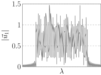
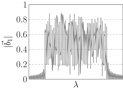
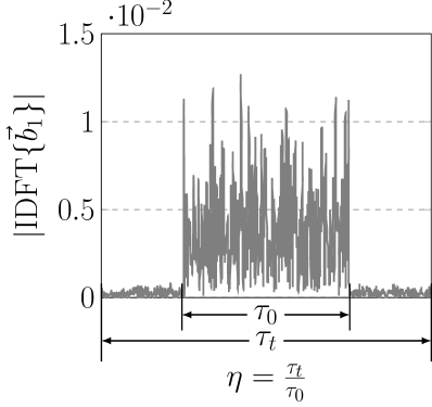
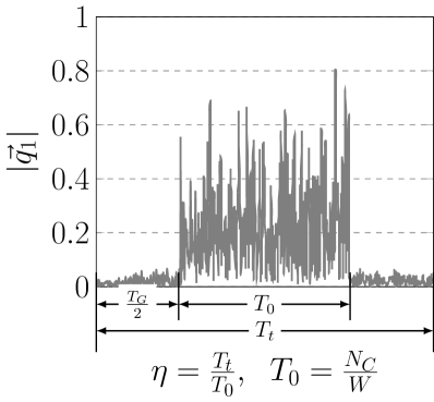
(a)    (b)    (c)    (d)

(e)

Figure 2: A realisation of signal at different stages of INFT-signal generation without pre-dispersion compensation. (a) OFDM spectrum as $\vec{u}_{1}$, (b) $\vec{b}_{1}$ spectrum when applying the transformation $\Gamma_{b}$ on $\mathbf{u}$, (c) IDFT of $\vec{b}_{1}$ with tails due to the transformation $\Gamma_{b}$, (d) time-domain signal generated by INFT. (e) Transceiver digital signal processing structure.

Figure 3: Simulation diagram of (a) $b$- or (b) $q_{c}$-modulated DP-NFDM systems. $\vec{Q_{b}}(t)$ and $\vec{Q_{c}}(t)$ are the time-domain signals of each system.

For any $\lambda\in\mathbb{R}$, the constraint $|b_{1}(\lambda)|^{2}+|b_{2}(\lambda)|^{2}<1$ specifies a 4-dimensional unit ball. The transformation $\Gamma_{b}$ facilitates the signal modulation on $b$-domain as it maps the entire $\mathbb{R}^{4}$ into this unit ball. Therefore, it allows using any arbitrary constellation format, e.g. QAM or equi-distance ring constellations without any concern on violating the constraint on $b$-coefficients. However, the transformation $\Gamma_{b}$ has a drawback. As it is shown in [12], modulating directly $b$-coefficients allows a full control on the duration of NFDM signals in time-domain. Applying non-linear transformations like $\Gamma_{b}$ causes losing this property to some extent. Nevertheless, this may not be practically a big issue. Although the generated NFDM signal may have some undesired tails, the tails are partially covered by the necessary long GI (specially after PDC) when the fibre length is long enough. Note that the longer GI is, the more ASE noise is taken into the NFT process, causing Q-factor degradation. The optimal GI that balances the extra ASE noise and the truncation of decaying tails is close to the estimated $T_{G}$ in (6).

Directly modulating $b$-coefficients of SP-NFDM was investigated in [13, 14]. In [13], the clipping technique was applied to satisfy the constraint on $b(\lambda)$. Clipping, an non-invertible operation commonly used for the peak-to-average power ratio (PAPR) reduction in OFDM systems [27, Sec. V-A], inevitably introduces distortion in $b(\tau)$ and cannot lift the constraint completely. In [14], another alternative was proposed to guarantee the constraint on $b$-coefficients by optimising the carrier waveform and applying constellation shaping. The technique was applied for 9 sub-carriers. It is of practical interest how the design complexity and the achievable SE scale for large number of sub-carriers. Moreover, the above techniques were presented in single polarisation. It is of interest how the joint constraint on $b_{1}(\lambda)$ and $b_{2}(\lambda)$ in dual polarisation, which limits independent modulation of $b_{1}(\lambda)$ and $b_{2}(\lambda)$, may affect the application of both techniques.

We demonstrate now the advantage of $b$-modulation over $q_{c}$-modulation in a relatively ideal case having a large guard interval $\eta=4\leavevmode\nobreak\ (N_{C}=70)$. The transmission of corresponding NFDM symbols are compared in two different simulated transmission scenarios: 1) the transmission over 12 spans of 80 km SSMF with EDFA amplification as illustrated in Fig. 3. It was simulated by the split-step Fourier method (SSFM) [29] using the parameters in Tab. I. 2) the additive white Gaussian noise (AWGN) channel without fibre transmission (back-to-back). The total additive noise powers were the same in both scenarios. Fig. 4 shows the clear advantage of $b$-modulation over $q_{c}$-modulation in both scenarios. Extra Q-factor degradation in the fibre transmission is attributed to the approximation error of the path-averaged model. The power $\mathcal{P}$ reported in this work is always the average power per polarisation.

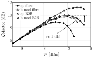
Figure 4: Q-factor vs. signal launch power in $q_{c}$- and $b$-modulated DP-NFDM systems with a large guard interval $\eta=4$ in both AWGN case and fibre transmission. The total additive noise powers are the same.

IV Optimisation of $b$-modulated DP-NFDM Transmission

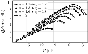
(a)

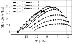
(b)

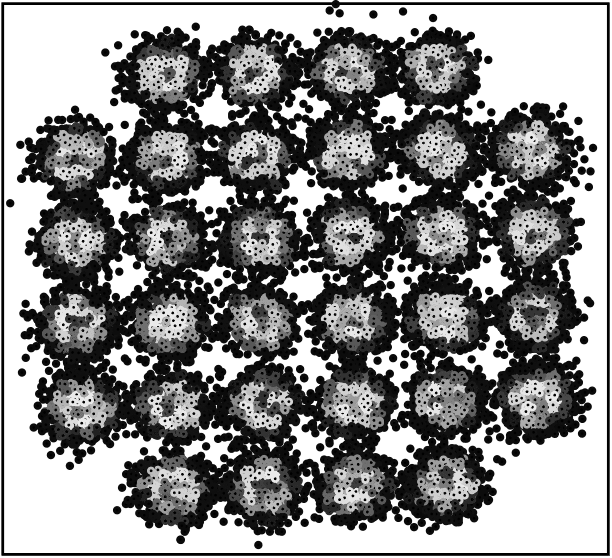
(c) (d)

Figure 5: The impact of decreasing $\eta$ on (a) Q-factor and (b) SE in $b$-modulated DP-NFDM system for different launch powers. $N_{C}=210/(\eta-1)$. The corresponding received constellation at the power of the maximum Q-factor (c) and SE (d).

Once the advantage of $b$-modulation is established, we optimise the $b$-modulated DP-NFDM system in terms of net data rate for the transmission scenario over $12\times 80$ km SSMF with EDFAs, visualised in Fig. 3. The optimisation parameters are the ratio $\eta$ and launch power per polarisation $\mathcal{P}$. The number of sub-carriers $N_{C}$ and $\eta$ are connected by

$$\eta=(T_{0}+T_{G})/T_{0}=1+WT_{G}/N_{C},$$

where $T_{G}=3.75$ ns and $W$ is fixed. For instance, it results $N_{C}=210$ for $\eta=2$. For each pair of $(\eta,\mathcal{P})$, the transmission of the corresponding NFDM symbols was simulated according to the parameters in Tab. I. For each NFDM symbol, the sub-carriers were detected individually and the performance was averaged over a large number of randomly generated NFDM symbols. To compute the SE, we estimate the mutual information (MI) (of individual sub-carrier detection) by assuming the channel conditional distribution as a Gaussian distribution [30, Sec. VI][31]. This assumption underestimates the correct MI and serves as an achievable information rate. The SE is then computed by

$$\textnormal{SE}=\frac{\textnormal{MI}\cdot N_{C}}{(T_{0}+T_{G})W}=\textnormal{MI}/\eta\leavevmode\nobreak\ (\rm bits/s/Hz/Pol.).$$

The computation of SE is to be taken in caution as we do not consider the spectral broadening of the signal in the fibre channel. We expect that decreasing $\eta$ will increase SE as well as the signal-noise interaction for a given launch power $\mathcal{P}$. For different values of $\eta$, the transmission performance metric Q-factor is plotted in Fig. 5(a) and SE in Fig. 5(b). They show respectively that Q-factor decreases monotonically as $\eta$ decreases, while SE reaches its maximum at $\eta=1.2$. Two received constellations at the power of the maximum Q-factor and SE are also plotted in Fig. 5(c) and 5(d). For $\eta=1.2$ ($N_{C}=1050$), and at power $\mathcal{P}=-8$ dBm per polarisation, we achieved a SE of $3.6$ bits/s/Hz/pol, resulting $400$ Gbps net data rate, while the gross data rate is $560$ Gbps. For the sake of comparison, we repeat the simulation for $q_{c}$-modulated DP-NFDM systems and plotted the SE curves in Fig. 6.

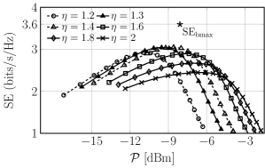
Figure 6: The impact of decreasing $\eta$ on SE in $q_{c}$-modulated DP-NFDM system for different launch powers. $N_{C}=210/(\eta-1)$.

V Co-variance Matrix of $q_{c}$- and $b$-modulated signals

In this section, we give some insights why the $b$-modulation scheme outperforms the $q_{c}$-modulation scheme. Let us first justify verbally. As we mentioned in Sec. II, there is a one-to-one correspondence between $\vec{b}(\lambda)$ and $\vec{q}_{c}(\lambda)$ provided that $\vec{b}(\lambda)\leavevmode\nobreak\ \textnormal{or}\leavevmode\nobreak\ \vec{q}_{c}(\lambda)\leavevmode\nobreak\ \forall\lambda\in\mathbb{R}$ and all discrete eigenvalues $\{\lambda_{m}\}$ are known. Therefore, $\vec{b}(\lambda)\leavevmode\nobreak\ \forall\lambda\in\mathbb{R}$ carries the same amount of information as $\vec{q}_{c}(\lambda)$ if the correlation between spectral coefficients, in either $\vec{b}(\lambda)$ or $\vec{q_{c}(\lambda)}\leavevmode\nobreak\ \forall\lambda\in\mathbb{R}$, can be fully exploited and no discrete eigenvalue emerges. However, our two DP-NFDM schemes have different performance for the following reasons:

• The sub-carriers are detected individually, where the correlation between sub-carriers is neglected. Strong correlations between sub-carriers cause then a large performance degradation.

• The two DP-NFDM schemes use the same modulation technique, i.e. OFDM with 32-QAM modulated sub-carriers. Depending on the distribution of noisy received data, this particular modulation format can be more resilient against noise for one scheme than the other.

We focus here on the first item, the correlation between sub-carriers. We show that the sub-carriers of $b$-modulated DP-NFDM system have much less correlation than the ones of $q_{c}$-modulated DP-NFDM system. To quantify all correlation coefficients with a single meaningful scalar, we use the differential entropy. We compare two quantities: the joint entropy which takes the correlations into account and the individual entropy which neglects the correlations. The gap between these quantities reflects how much the sub-carriers are correlated and how much the net data rate will be decreased (to some extent) by neglecting the correlations.

For both DP-NFDM systems, we numerically compute the differential entropies. Let $\vec{X}=[X_{1}\leavevmode\nobreak\ X_{2}\leavevmode\nobreak\ ...\leavevmode\nobreak\ X_{2N_{C}}]$ denote the randomly chosen 32-QAM data modulated on $2N_{C}$ sub-carriers (DP). Let $\vec{Y}=[Y_{1}\leavevmode\nobreak\ Y_{2}\leavevmode\nobreak\ ...\leavevmode\nobreak\ Y_{2N_{C}}]$ denote the received noisy data of sub-carriers after the NFT processing. The joint entropy is defined as

$$h(\vec{Y}|\vec{X}) =\frac{1}{4N_{C}}\mathbb{E}_{\vec{x}}\left(h(\vec{Y}|\vec{X}=\vec{x})\right)$$

where $h(\vec{Y}|\vec{X}=\vec{x})$ is the entropy of received data given $\vec{x}$, a realisation of inputs $\vec{X}$. $\mathbb{E}_{\vec{x}}$ denotes taking expectation over all realisations of $\vec{x}$. The individual entropy is defined as

$$h_{\Sigma}(\vec{Y}|\vec{X}) =\frac{1}{4N_{C}}\mathbb{E}_{\vec{x}}\left(\sum_{i=1}^{2N_{C}}h(Y_{i}|\vec{X}=\vec{x})\right)$$

where $h(\vec{Y_{i}}|\vec{X}=\vec{x})$ is the entropy of the individual received sub-carrier $Y_{i}$ given the realisation $\vec{x}$. To compute the above quantities, we need the conditional probability density $f({\vec{Y}|\vec{X}})$. It is, however, unknown yet for NFDM systems and difficult to estimate due to its large dimension $4N_{C}$. We approximate $f({\vec{Y}|\vec{X}})$ by a complex multivariate Gaussian distribution. We justify our choice later in Remark 1. Define $\vec{W}=[\text{Re}(\vec{Y}),\text{Im}(\vec{Y})]$, then the corresponding probability density $f({\vec{W}|\vec{X}})$ is approximated by a real-valued multivariate Gaussian distribution with covairance matrix $\mathbf{K}$. The element of $\mathbf{K}$ is defined as

$$k_{ij}=\mathbf{E}[(W_{i}-\mathbf{E}[W_{i}])(W_{j}-\mathbf{E}[W_{j}])].$$

In this case, the conditional entropies can be approximated as

$$h(\vec{Y}|\vec{X}=\vec{x}) \approx\frac{1}{8N_{C}}\log\left(\det\left(2\pi e\mathbf{K}\right)\right),$$ (7)

$$h_{\Sigma}(\vec{Y}|\vec{X}=\vec{x}) \approx\frac{1}{8N_{C}}\log(\prod_{i=1}^{2N_{C}}2\pi ek_{ii}).$$ (8)

We estimated $\mathbf{K}$ for each realisation $\vec{x}$ from simulated data. We simulated the fibre transmission scenario visualised in Fig. 3 for both DP-NFDM systems. We set $\eta=2$, resulting $N_{C}=210$ sub-carriers. For each DP-NFDM system, we randomly generated 20 input realisations $\vec{x}$. For each realisation, the transmission of its corresponding DP-NFDM symbol was simulated $2^{14}$ times with different random noise realisations. The simulation is repeated for different launch powers $\mathcal{P}$. Accordingly, the above entropies are computed from the resulted $\mathbf{K}$ for each input realisation $\vec{x}$. Fig. 7(a) shows the entropies of each realisation $\vec{x}$ for both DP-NFDM systems at launch power $\mathcal{P}=-3.75$ dBm. We observe that the curves have small variations for different realisations $\vec{x}$. We finally estimated $h(\vec{Y}|\vec{X})$ and $h_{\Sigma}(\vec{Y}|\vec{X})$ by the empirical average of 20 input realisations.

Fig. 7(b) illustrates the conditional entropies in terms of launch power for both DP-NFDM systems. We observe that the gap $h(\vec{Y}|\vec{X})-h_{\Sigma}(\vec{Y}|\vec{X})$ is smaller for the $b$-modulated scheme than the one for the $q_{c}$-modulated scheme. It implies that the penalty of individual detection is smaller for the $b$-modulated scheme. For both schemes, the increase of the gap in terms of launch power implies that the sub-carriers becomes more correlated for larger $\mathcal{P}$. Moreover, $h(\vec{Y}|\vec{X})$ of the $b$-modulated scheme is not only smaller but also has a slower growth in terms of $\mathcal{P}$. It indicates that in comparison of both systems, the co-variance matrix $\mathbf{K}$ of the $b$-modulated scheme has, on average, smaller diagonal elements which grow also slower in $\mathcal{P}$. In plain language, the “effective noise” contaminating $b$-modulated scheme has smaller power and its power grows also slower with increasing $\mathcal{P}$ than the one of $q_{c}$-modulation. Let us emphasise that the constellation of both DP-NFDM systems are the same in $u(\lambda)$ domain (shown in Fig. 3) for a fair comparison in Fig. 7(b).

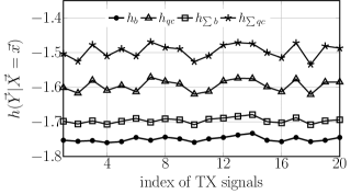
(a)

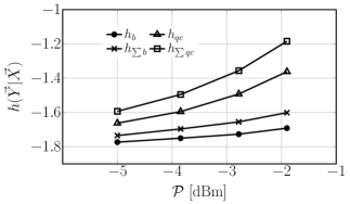
(b)

Figure 7: Conditional differential entropy of received symbols in both $q_{c}$ and $b$-modulated DP-NFDM systems with the assumption of Gaussian distribution, for different transmitted symbols (a) and powers (b).

Remark 1. To verify the validity of entropy approximations, we further applied the entropy estimator in [32], which can rather precisely estimate the differential entropy of a low-dimensional random variable from its random samples. To have robust estimations, we estimated the differential entropies of only 10 adjacent sub-carriers (20 real-valued dimensions). For different input realisation $\vec{x}$, we observed that the estimations are fairly close to the corresponding entropies of the Gaussian approximation, as shown in Fig. 8.

Remark 2. Comparing both DP-NFDM systems in terms of correlation and conditional entropy is more qualitative than quantitative. The joint MI between transmitted and received data on all sub-carriers is the suitable metric to “quantify” the performance difference of both NFDM schemes (with joint detection). The MIs using individual detection are already compared in Sec. IV. However, the joint MI requires $f(\vec{Y}|\vec{X})$ as well as the probability density $f(\vec{Y})$. It is more challenging to estimate $f(\vec{Y})$ specially when the input $\vec{X}$ is drawn from a discrete constellation, e.g., 32-QAM in our case. The probability density $f(\vec{Y})$ is a multi-dimensional multi-center distribution, with correlation between dimensions. The entropy $H(\vec{Y})$ is nearly impossible to calculate. Hence, this problem makes the estimation of MI (jointly between all sub-carriers) much more challenging.

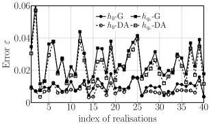
Figure 8: The relative error between distribution-agnostic entropy estimator [32] and the Gaussian entropy for 10 adjacent sub-carriers. G stands for Gaussian entropy, DA for distribution-agnostic entropy estimation. For both methods, the result of one-dimensional entropy $h(Y_{i}|\vec{x})$ is very close. $\varepsilon=\big{(}\sum_{i=1}^{10}h(Y_{i}|\vec{x})-h(Y_{1},...,Y_{10}|\vec{x})\big{)}/\sum_{i=1}^{10}h(Y_{i}|\vec{x})$

.

VI Some Drawbacks of the Current System

Based on the above simulation results, we identified two main sources of error in our current system: ‘transceiver distortion’ in noiseless back-to-back scenario and channel mismatch owing to its non-integrability.

VI-A Transceiver Distortion in Noiseless Back-to-Back Scenario

The transceiver distortion includes the distortion from the whole digital signal processing shown in Fig. 2(e), such as the inaccuracy of the INFT-NFT algorithm, the application of $\Gamma_{b}$ and the truncation of time-domain signal. Their overall effect can be easily quantified in an noiseless back-to-back simulation of the $b$-modulated DP-NFDM system. Fig. 9 shows the Q-factor in terms of average energy per NFDM symbol for different $\eta$ in . The average energy of one NFDM symbol can be calculated by $\mathcal{P}(T_{0}+T_{G})=\mathcal{P}\eta N_{C}/W$. It shows clearly that the transceiver distortion is energy-dependent.

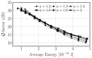
Figure 9: ‘Transceiver distortion’ in the $b$-modulated DP-NFDM system in the noiseless back-to-back scenario. The average energy of NFDM symbol is calculated by $\mathcal{P}(T_{0}+T_{G})=\mathcal{P}\eta N_{C}/W$.

VI-B Channel Mismatch due to Non-integrability

NFT is only exact for integrable channels such as (2). To successfully apply NFT to the non-integrable channel (1), an approximation step has to be taken. To quantify the approximation distortion, one should simulate noiseless systems in Fig. 3 with a transceiver DSP that does not cause any distortion. This is unfeasible with our current transceiver DSP. To adopt a different approach, we first clarify the concepts of different digital back-propagation (DBP) schemes, as DBP is the main tool in our error quantification.

We recall the Manakov equation (1). The ideal DBP refers to the process of solving the Manakov equation to recover $\vec{Q}(0,t)$ (input) from the boundary condition $\vec{Q}(z,t)$ (output), using SSFM with fine step size (0.1 km). The EDFAs are replaced with attenuators of the opposite gain. In a single-channel scenario, the ideal DBP should fully cancel the deterministic distortion.

We recall also the integrable path-averaged Manakov equation (2). The path-averaged DBP refers to the process of solving the path-averaged Manakov equation to recover $\vec{Q}(0,t)$ from the boundary condition $\vec{Q}(z,t)$, using SSFM with fine step size (0.1 km). Since the signal propagation occurs in the Manakov equation, applying path-averaged DBP inevitably causes distortion on the recovered signal $\vec{Q}(0,t)$ even in the single-channel scenario.

In single-channel scenario, if viewed as a compensation scheme, the combination of NFT, back-rotation in non-linear frequency domain, and INFT is somewhat equivalent to the path-averaged DBP. Therefore, we propose to use the residual distortion in a noiseless non-integrable system that is compensated by path-averaged DBP to estimate the approximation distortion. Fig. 10(a)(b) describe two noiseless systems with ideal and path-averaged DBP compensation, using the parameters in Tab. I. These systems employ dual polarisation 32-QAM Nyquist signal with 56 GHz bandwidth. In general, any signal whose transceiver DSP causes no distortion suits the purpose. The residual distortion of the system (a) in Fig. 10 is considered equivalent to the approximation distortion in systems of Fig. 3. Fig. 10(c) shows that in the power range of our interest ( $\leq-0$ dBm), the approximation distortion is negligible.

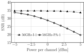
(c)

Figure 10: (a)(b) Simulation diagram of non-integrable models. PA-DBP stands for path-averaged DBP, IDBP for ideal DBP, COI for channel-of-interest. (c) residual distortion of IDBP (shortened in the legend to I, preceded by total bandwidth and followed by number of channels) and PA-DBP (shortened in the legend to PA) systems.

VII Conclusions

The previous work [33] is extended here with more analysis on the correlation, joint and individual entropy of $b$-modulated signals. The results confirmed the viability and benefits of the $b$-modulation in the DP-NFDM system.

The $q_{c}$- and $b$-modulated DP-NFDM systems were compared in terms of Q-factor, correlation of sub-carriers, joint and individual entropy. The $b$-modulated DP-NFDM system shows 1 dB Q-factor improvement over $q_{c}$-modulated DP-NFDM system due to a weaker correlation of sub-carriers and less effective noise. At last, the $b$-modulated system was optimised for higher data rate, achieving a record net data rate of 400 Gbps (SE of 7.2 bit/s/Hz) on the SSMF with EDFAs over $12\times 80$ km.

References

- [1] M. Yousefi and X. Yangzhang, “Linear and nonlinear frequency-division multiplexing,” in Eur. Conf. Opt. Commun. (ECOC), (Düsseldorf, Germany), Sept 2016.
- [2] R. J. Essiambre, G. Kramer, P. J. Winzer, G. J. Foschini, and B. Goebel, “Capacity limits of optical fiber networks,” J. Lightw. Technol., vol. 28, pp. 662–701, Feb 2010.
- [3] M. I. Yousefi and F. R. Kschischang, “Information transmission using the nonlinear Fourier transform, Part I: Mathematical tools,” IEEE Trans. Inf. Theory, vol. 60, pp. 4312–4328, July 2014.
- [4] X. Yangzhang, D. Lavery, P. Bayvel, and M. Yousefi, “Impact of perturbations on nonlinear frequency-division multiplexing,” J. Lightw. Technol., vol. 36, pp. 485–494, Jan 2018.
- [5] V. Aref, S. T. Le, and H. Buelow, “Modulation over nonlinear fourier spectrum: Continuous and discrete spectrum,” J. Lightw. Technol., vol. 36, pp. 1289–1295, Mar 2018.
- [6] S. T. Le, V. Aref, and H. Buelow, “High speed precompensated nonlinear frequency-division multiplexed transmissions,” J. Lightw. Technol., vol. 36, pp. 1296–1303, Mar 2018.
- [7] W. Gemechu, M. Song, Y. Jaouen, S. Wabnitz, and M. Yousefi, “Comparison of the Nonlinear Frequency Division Multiplexing and OFDM in experiment,” in Eur. Conf. Opt. Commun. (ECOC), (Gothenburg, Sweden), p. W.3.C.4, Sept 2017.
- [8] S. Civelli, J. E. Prilepsky, M. Secondini, and S. K. Turitsyn, “Polarization division multiplexing for nonlinear fourier-based transmission schemes,” in Conference on Lasers and Electro-Optics, (San Jose, CA, USA), p. STu4C.4, 2018.
- [9] I. Tavakkolnia and M. Safari, “Signaling on the continuous spectrum of nonlinear optical fiber,” Opt. Express, vol. 25, pp. 18685–18702, Aug 2017.
- [10] S. Le, V. Aref, and H. Buelow, “Nonlinear signal multiplexing for communication beyond the Kerr nonlinearity limit,” Nat. Photon., vol. 11, pp. 570–576, July 2017.
- [11] S. K. Turitsyn, J. E. Prilepsky, S. T. Le, S. Wahls, L. L. Frumin, M. Kamalian, and S. A. Derevyanko, “Nonlinear fourier transform for optical data processing and transmission: advances and perspectives,” Optica, vol. 4, pp. 307–322, Mar 2017.
- [12] S. Wahls, “Generation of time-limited signals in the nonlinear fourier domain via b-modulation,” in Eur. Conf. Opt. Commun. (ECOC), (Gothenburg, Sweden), W.3.C.6, Sept 2017.
- [13] S. T. Le, K. Schuh, F. Buchali, and H. Buelow, “100 Gbps b-modulated nonlinear frequency division multiplexed transmission,” in Opt. Fiber Commun. Conf. (OFC), (San Diego, CA, USA), W1G.6, Mar 2018.
- [14] T. Gui, G. Zhou, C. Lu, A. P. T. Lau, and S. Wahls, “Nonlinear frequency division multiplexing with b-modulation: shifting the energy barrier,” Opt. Express, vol. 26, pp. 27978–27990, Oct 2018.
- [15] J.-W. Goossens, M. I. Yousefi, Y. Jaouën, and H. Hafermann, “Polarization-division multiplexing based on the nonlinear fourier transform,” Opt. Express, vol. 25, pp. 26437–26452, Oct 2017.
- [16] S. Civelli, E. Forestieri, and M. Secondini, “Decision-feedback detection strategy for nonlinear frequency-division multiplexing,” Opt. Express, vol. 26, pp. 12057–12071, Apr 2018.
- [17] W. A. Gemechu, T. Gui, J. Goossens, M. Song, S. Wabnitz, H. Hafermann, A. P. T. Lau, M. I. Yousefi, and Y. Jaouën, “Dual polarization nonlinear frequency division multiplexing transmission,” IEEE Photon. Technol. Lett., vol. 30, pp. 1589–1592, Sept 2018.
- [18] S. T. Le, H. Buelow, and V. Aref, “Demonstration of 640.5 Gbaud nonlinear frequency division multiplexed transmission with 32QAM,” in Optical Fiber Communication Conference, p. W3J.1, 2017.
- [19] S. T. Le and H. Buelow, “64 0.5 gbaud nonlinear frequency division multiplexed transmissions with high order modulation formats,” J. Lightwave Technol., vol. 35, pp. 3692–3698, Sept 2017.
- [20] G. P. Agrawal, “Nonlinear fiber optics,” pp. 193 – 244, Boston: Academic Press, Fifth ed., 2013.
- [21] A. Hasegawa and Y. Kodama, “Guiding-center soliton in optical fibers,” Opt. Lett., vol. 15, pp. 1443–1445, Dec 1990.
- [22] S. T. Le, J. E. Prilepsky, and S. K. Turitsyn, “Nonlinear inverse synthesis technique for optical links with lumped amplification,” Opt. Express, vol. 23, pp. 8317–8328, Apr 2015.
- [23] S. V. Manakov, “On the theory of two-dimensional stationary self-focusing of electromagnetic waves,” Soviet Journal of Experimental and Theoretical Physics, vol. 38, pp. 505–516, Feb. 1974.
- [24] M. Ablowitz and H. Segur, Solitons and the Inverse Scattering Transform. SIAM studies in applied and numerical mathematics: Society for Industrial and Applied Mathematics, SIAM, 1981.
- [25] L. Faddeev, A. Reyman, and L. Takhtajan, Hamiltonian Methods in the Theory of Solitons. Classics in Mathematics, Springer Berlin Heidelberg, 2007.
- [26] M. I. Yousefi and X. Yangzhang, “Linear and nonlinear frequency-division multiplexing,” arXiv:1603.04389v3, May 2016.
- [27] J. Armstrong, “OFDM for optical communications,” J. Lightw. Technol., vol. 27, pp. 189–204, Feb 2009.
- [28] I. Tavakkolnia and M. Safari, “Dispersion pre-compensation for NFT-based optical fiber communication systems,” in Conf. on Lasers and Electro-Optics (CLEO), (San Jose, CA, USA), SM4F.4, Jun 2016.
- [29] O. V. Sinkin, R. Holzlohner, J. Zweck, and C. R. Menyuk, “Optimization of the split-step fourier method in modeling optical-fiber communications systems,” J. Lightw. Technol., vol. 21, pp. 61–68, Jan 2003.
- [30] D. M. Arnold, H. . Loeliger, P. O. Vontobel, A. Kavcic, and W. Zeng, “Simulation-based computation of information rates for channels with memory,” IEEE Trans. Inf. Theory, vol. 52, pp. 3498–3508, Aug 2006.
- [31] A. Alvarado, T. Fehenberger, B. Chen, and F. M. J. Willems, “Achievable information rates for fiber optics: Applications and computations,” J. Lightwave Technol., vol. 36, pp. 424–439, Jan 2018.
- [32] D. Lombardi and S. Pant, “Nonparametric -nearest-neighbor entropy estimator,” Phys. Rev. E, vol. 93, p. 013310, Jan 2016.
- [33] X. Yangzhang, V. Aref, S. T. Le, H. Bülow, and P. Bayvel, “400 Gbps Dual-Polarisation Non-Linear Frequency-Division Multiplexed Transmission with B-Modulation,” in Eur. Conf. Opt. Commun. (ECOC), (Rome, Italy), We4F.1, Sept 2018.