Census of $\rho$ Oph candidate members from Gaia Data Release 2

Abstract

Context. The Ophiuchus cloud complex is one of the best laboratories to study the earlier stages of the stellar and protoplanetary disc evolution. The wealth of accurate astrometric measurements contained in the Gaia Data Release 2 can be used to update the census of Ophiuchus member candidates.

Aims. We seek to find potential new members of Ophiuchus and identify those surrounded by a circumstellar disc.

Methods. We constructed a control sample composed of 188 bona fide Ophiuchus members. Using this sample as a reference we applied three different density-based machine learning clustering algorithms (DBSCAN, OPTICS, and HDBSCAN) to a sample drawn from the Gaia catalogue centred on the Ophiuchus cloud. The clustering analysis was applied in the five astrometric dimensions defined by the three-dimensional Cartesian space and the proper motions in right ascension and declination.

Results. The three clustering algorithms systematically identify a similar set of candidate members in a main cluster with astrometric properties consistent with those of the control sample. The increased flexibility of the OPTICS and HDBSCAN algorithms enable these methods to identify a secondary cluster. We constructed a common sample containing 391 member candidates including 166 new objects, which have not yet been discussed in the literature. By combining the Gaia data with 2MASS and WISE photometry, we built the spectral energy distributions from $0.5$ $\mu\mathrm{m}$ to $22$ $\mu\mathrm{m}$ for a subset of 48 objects and found a total of 41 discs, including 11 Class II and 1 Class III new discs.

Conclusions. Density-based clustering algorithms are a promising tool to identify candidate members of star forming regions in large astrometric databases. By combining the Gaia data with infrared catalogues, it is possible to discover new protoplanetary discs. If confirmed, the candidate members discussed in this work would represent an increment of roughly $40-50\%$ of the current census of Ophiuchus.

1 Introduction

Star forming regions (SFR) composed of hundreds of pre-main sequence (PMS) stars are natural laboratories to learn about the early stages of the stellar evolution process. These places are crucial to study the birth sites of planets as a significant fraction of PMS stars are surrounded by protoplanetary discs. Understanding and identifying the mechanisms driving the evolution of these discs is key to explain how planetary systems are formed (e.g. Morbidelli & Raymond 2016). With this goal in mind several teams have observed large populations of protoplanetary discs in various SFRs across a range of wavelengths (e.g. Cieza et al. 2018; Dent et al. 2013; Evans et al. 2009; Haisch et al. 2001). Analyses of extensive disc samples (and their stellar hosts) have revealed trends such as the disc mass-stellar mass relation (Andrews et al. 2013; Ansdell et al. 2016; Pascucci et al. 2016) and the decrement of disc mass in millimeter-sized grains with stellar age (Ansdell et al. 2017; Ruíz-Rodríguez et al. 2018). A general limitation of these studies is the lack of a complete census of the members of the region under analysis. Such a census is also desirable (among many other reasons) to assess the impact of the environment over the observed disc properties because, for instance, stellar fly-bys are expected to affect disc sizes, shapes, and masses (Bate 2011, 2018; Cuello et al. 2019).

Identifying the members of any SFR is a difficult task hindered by various causes. Nearby (¡400 pc from Earth) regions generally occupy large areas ($\geq 1$deg²) on the projected sky, and therefore it is observationally expensive to study these regions with classical observatories. Furthermore, the late spectral type objects that populate these regions are difficult to detect and characterise as a consequence of their intrinsic lower luminosity, and the same applies to any young stellar object (YSO) that has a very high extinction. Early works took advantage of the strong X-ray activity and accretion driven $\mathrm{H}_{\alpha}$ emission of PMS stars to detect these objects using X-ray observatories and $\mathrm{H}_{\alpha}$ objective prism surveys (e.g. Montmerle et al. 1983; Walter et al. 1994; Wilking et al. 1987). More recently, the use of astrometric measurements has made it possible to identify or confirm hundreds of members of several SFRs and young associations using different methods (Bruijne 1999; Malo et al. 2013; de Zeeuw et al. 1999). The advent of the Gaia mission (Gaia Collaboration et al. 2016) is revolutionising this (and many other) field(s), allowing for the detection of new candidate members of different stellar populations by means of accurate astrometric measurements. In a few remarkable cases, a direct inspection by eye of the Gaia astrometry can even reveal the members of a stellar cluster (e.g. the Pleiades example in Brown et al. 2016; Taylor 2017). However, in practice complex algorithms are needed to identify the member candidates based on the astrometric properties of the studied sample (e.g. Gagné et al. 2018). This becomes increasingly difficult when processing large catalogues such as the Gaia Data Release 2 (DR2; Lindegren et al. 2018).

The so-called unsupervised machine learning (ML) clustering algorithms are a collection of software tools developed to identify patterns or clusters in unlabelled databases. Within these algorithms there are multiple approaches to the problem of cluster detection, such as centroid-based algorithms (e.g. the $k$-means algorithm; Lloyd 1982), distribution-based clustering (e.g. Gaussian-mixture models), or density-based algorithms (for an overview of clustering analysis in astronomy see e.g. Feigelson & Babu 2012, their Chapter 3.3 and references therein). The latter are well-suited to identify arbitrarily shaped clusters that can be broadly described as overdensities in a lower density space. An advantage of the density-based algorithms is that no prior knowledge about the analysed dataset is needed. In other words, the user does not need to know the number of clusters present in the dataset, and these algorithms do not assume any particular distribution (such as one or multiple Gaussians) when associating the data points with a cluster. Density-based spatial clustering of applications with noise (DBSCAN; Ester et al. 1996) stands out as one of the most famous algorithms in many disciplines, and it is becoming popular in astronomy (e.g. Beccari et al. 2018; Bianchini et al. 2018; Caballero & Dinis 2008; Castro-Ginard et al. 2018; Joncour et al. 2018; Hague et al. 2019; Tramacere & Vecchio 2013; Wilkinson et al. 2018). There are a number of modifications or improvements of DBSCAN and, among those, the ordering points to identify the clustering structure (OPTICS; Ankerst et al. 1999) and the hierarchical density-based spatial clustering of applications with noise (HDBSCAN; Campello et al. 2013) algorithms are becoming popular owing to their recognised performance to detect various types of clusters. However, to date their use in the astronomical literature is still negligible except for a few cases (e.g. Costado et al. 2017; Katz et al. 2017; Kimm et al. 2018; Sans Fuentes et al. 2017).

In this paper we use the DBSCAN, OPTICS, and HDBSCAN algorithms to identify potential members of the Ophiuchus SFR (hereafter $\rho$ Oph) in a sample drawn from the Gaia DR2 catalogue (Brown et al. 2018). With average distance and age estimates ranging from 120 pc to 140 pc and 2 Myr to 5 Myr, respectively (Wilking et al. 2008, and references therein), $\rho$ Oph has been the subject of numerous studies (e.g. Andrews et al. 2009; Andrews & Williams 2007; Cheetham et al. 2015; Cox et al. 2017; Erickson et al. 2011; Mamajek 2008; Wilking et al. 2008). Recently, 289 discs in this cloud have been observed with ALMA aiming to study in detail the different evolutionary stages of the protoplanetary discs (Cieza et al. 2018). The $\rho$ Oph region is located at the foreground of the southeastern edge of the Upper Scorpius (hereafter USco) subgroup of the large Sco-Cen OB association (de Geus et al. 1989; de Zeeuw et al. 1999). Both USco and $\rho$ Oph have similar proper motion distributions (Mamajek 2008), and it has been proposed that the star formation in $\rho$ Oph was triggered by a supernova event in USco (de Geus 1992; Erickson et al. 2011; Preibisch et al. 2002). A major difference between both regions is their age and evolutionary stage. While the $\rho$ Oph region is rich in molecular gas, has a very high optical extinction, and star formation is still ongoing, the opposite is found in the $\sim 10$ Myr old USco (Pecaut et al. 2012; Pecaut & Mamajek 2016; Wilking et al. 2008). Given the youth of $\rho$ Oph, its members have similar velocity distributions and they are concentrated in a relatively compact region of the Galaxy. In other words, the cloud members should appear clustered in the multi-dimensional space defined by their spatial coordinates and kinematic parameters when compared to the field stellar population. We applied the clustering algorithms in the five-dimensional space defined by the three spatial coordinates and two kinematical parameters given by the proper motions on right ascension $\,\mu_{\alpha^{*}}$ and declination $\,\mu_{\delta}$. By comparing their results we aim to reduce the selection biases inherent to each algorithm and therefore construct a robust sample of $\rho$ Oph members candidates. The samples used for our study are described in Section 2. In Section 3 we describe our methodology and apply the three algorithms to our Gaia sample. This section finishes by presenting a sample of sources simultaneously identified by the three algorithms. In Section 4 we discuss the properties of this sample and we use infrared photometry to identify a set of objects showing warm dust emission associated with a circumstellar disc. A summary and conclusions are given in Section 5, while extra figures and tables are shown in the Appendix.

2 Sample construction

2.1 Initial sample

We begun by compiling a list of $\rho$ Oph member candidates identified as such by means of optical spectroscopy, X-ray emission, or Spitzer photometry. To do so we considered the 316 objects listed by Wilking et al. (2008), the sample discussed by Erickson et al. (2011) (135 objects), and the catalogue of $\rho$ Oph YSO candidates observed by Spitzer during the Cores to Disks Legacy program (Evans et al. 2003) and presented by Dunham et al. (2015) (292 objects). The on-line versions of these catalogues, hosted by the VizieR service, include a SIMBAD (Wenger et al. 2000) ID associated with each object. We used these IDs to obtain the corresponding Two Micron All Sky Survey (2MASS; Skrutskie et al. 2006) IDs. There are no 2MASS counterparts for 2 objects in the Wilking et al. (2008) catalogue, 1 object from Erickson et al. (2011), and 10 objects from Dunham et al. (2015), and these 13 sources are not considered in our study. After accounting for duplicates we obtained our initial sample, which contains 465 objects. This sample is listed in Table 6 in the Appendix.

2.2 Control sample

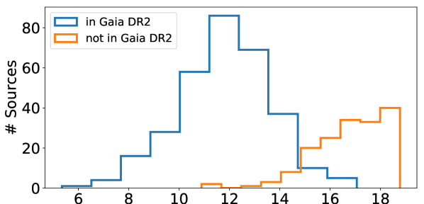
Figure 13: Apparent $J$ band magnitude histograms of the initial sample.

With the 2MASS IDs of our initial sample at hand we run an identity cross-match Astronomical Data Query Language (ADQL; Osuna et al. 2008) query between our initial sample and the Gaia DR2 catalogue using the 2MASS-Gaia matched table (gaiadr2.tmass_best_neighbour) available on the Gaia archive. This approach is advantageous compared to a sky cross-match by coordinates as there is no need to transform the 2MASS coordinates from the J2000 to the J2015.5 epoch. Our query returned 304 sources. The missing objects are generally fainter at $J$ band (and therefore probably fainter at $G$ band) than the detected objects (see Fig. 13 in the Appendix). The results listed on the DR2 catalogue (such as the right ascension $\,\alpha$, the declination $\,\delta$, the parallax $\,\varpi$, and the proper motions in right ascension and declination $\,\mu_{\alpha^{*}}$ and $\,\mu_{\delta}$) are obtained through a complex data analysis process that relies on treating each observed source as a single, “well behaved” star (the five-parameter model; see Lindegren et al. 2012, 2018). Binaries and YSOs, which are typically variable and can appear as extended sources at optical wavelengths, can be problematic for the astrometric solution. Therefore, we applied a selection criteria to extract the sources with high quality astrometry. First, we removed the objects with parallax signal to noise $\varpi/\sigma_{\varpi}<10$ and visibility periods $\leq 7$ to produce an astrometrically precise and reliable dataset (see Lindegren et al. 2018; Arenou et al. 2018). Second, we only extracted the sources whose observations are consistent with the five-parameter model. To do so, we applied the current quality criteria described in the Gaia technical note GAIA-C3-TN-LU-LL-124-01 that is based on an empirical analysis of the Gaia DR2 data. This analysis introduces the renormalised unit weight error (RUWE), which is a reliable indicator of the goodness-of-fit of the astrometric solution. Using the RUWE as a quality index is especially useful for samples containing very red stars, such as the low-mass and extinct PMS stars in $\rho$ Oph. We extracted the sources with RUWE $<1.40$ as recommended by this study.

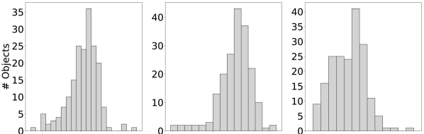
Figure 15: Same as Fig. 14 but for the control sample (obtained after removing the outliers listed in Table 7 from the astrometrically cleaned sample).

This astrometrically cleaned sample contains 197 objects. We generated its histogram distributions over $\,\varpi$, $\,\mu_{\alpha^{*}}$, and $\,\mu_{\delta}$, applying the Bayesian approach derived by Knuth (2006) that optimises the bin widths based on the data distribution and that is implemented in Astropy (Robitaille et al. 2013). Throughout this paper we use mas and mas yr^-1 as the reference units for the parallaxes and proper motions, respectively, and all the histograms are constructed by applying the same methodology. These histograms show bell-shaped distributions with a few objects located far away from the histogram peaks (Fig. 14). We removed these outliers by considering only the objects with $5<$$\,\varpi$ $<9$ and $-20<$$\,\mu_{\alpha^{*}}$ $<0$. The 9 objects excluded by this filter are listed in Table 7 in the Appendix. Given their parallaxes and proper motions we consider these as background objects instead of $\rho$ Oph members. Our final sample, hereafter called control sample, contains 188 targets. There are Gaia radial velocities for 7 of the objects, which have an average value of $v_{\mathrm{rad}}=-7.7\pm 2.4\,\mathrm{km\,s}^{-1}$. This sample occupies a sky region extending from $[245.3\degr:249.9\degr]$ in right ascension and $[-25.4\degr:-22.9\degr]$ in declination, and has an average parallax of $\,\varpi$ $=7.1\pm 0.4$. The average astrometric properties of the control sample are listed in Table 1 and its parallax and proper motion histograms are shown in the Appendix (Fig. 15). Following Bailer-Jones (2015) we computed the individual distances as $d=1/\varpi$ since the parallax fractional error of this sample is lower than 10. This way we obtained an average distance of $d=141.2_{-7.5}^{+8.4}$ pc to this sample, where the uncertainty is dominated by the intrinsic dispersion of the dataset. In short, this sample contains 188 bonafide members of the $\rho$ Oph cloud that can be used as a reference sample. The control sample members are labelled in Table. 6 with a ”Y” in the control column.

Stats	$\,\alpha$	$\,\delta$	$\,\varpi$	$\,\mu_{\alpha^{*}}$	$\,\mu_{\delta}$
	[∘]	[∘]	[$\mathrm{mas}$]	[$\mathrm{mas\,yr^{-1}}$]	[$\mathrm{mas\,yr^{-1}}$]
Mean	246.8	-24.3	7.1	-7.2	-25.5
Sigma	0.6	0.5	0.4	2.0	1.7

Table 1: Mean and standard deviation ($1\sigma$) of the control sample.

2.3 Gaia sample

In order to create a large sample to search for potential new members of $\rho$ Oph we run an ADQL cone search on the Gaia server centred at $[247.0\degr,-24.0\degr]$ in $[\alpha,\delta]$ with a search radius of $r=3.5\degr$ chosen to generously encompass the control sample (see Fig. 1). We imposed a parallax range from $[5:9]$ and parallax signal to noise S/N $>10$. This query returned 2814 targets that were reduced to 2300, including the 188 objects of the control sample, after applying the quality selection criteria described in Sect. 2.2. This sample, labelled hereafter as the Gaia sample, contains radial velocity values for 236 sources with an average value of $v_{\mathrm{rad}}=-6.9\pm 31.8\,\mathrm{km\,s}^{-1}$. Figure 2 shows a zoom in of the $\,\mu_{\alpha^{*}}$ versus $\,\mu_{\delta}$ of the Gaia sample; the control sample members are overlaid on top as small magenta circles. There is an evident overdensity of sources around the centre of the plot. This overdensity seems to contain two different regions or clusters: one with most of its members located around $[-7.5,-25]$, and the second roughly centred at $[-12,-21]$ in [$\,\mu_{\alpha^{*}}$, $\,\mu_{\delta}$ ]; these are labelled as “Cluster 1” and “Cluster 2” in Fig. 2, respectively. The control sample members are mostly concentrated in Cluster 1.

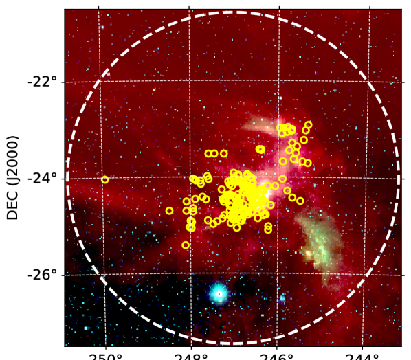
Figure 1: WISE image of the $\rho$ Oph region in a square-root stretched scale with RGB colours mapped to 22, 4.6, and 3.4 $\mu$m. The control sample members are represented as yellow rings. The white dashed ring encompasses the area queried in the Gaia server. The saturated blue star towards the south is $\alpha$ Scorpii (a.k.a. Antares).

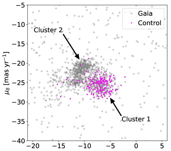
Figure 2: Zoom-in of the proper motions of the Gaia sample represented with grey circles. Their diameter roughly equals the average error on $\,\mu_{\alpha^{*}}$ (0.35 mas yr^-1), which is larger than the average error in $\,\mu_{\delta}$ (0.23 mas yr^-1). The control sample members are represented as small magenta circles.

3 Analysis

3.1 Basic concepts of density-based clustering

It is not straightforward to discriminate between the diffuse cluster(s) with no sharp boundaries and the population of background or foreground objects shown in Fig. 2. As mentioned in the introduction, there are multiple software tools that are able to identify clusters embedded in large databases. We chose to use the family of density-based clustering algorithms because they are especially well suited to detect arbitrarily shaped clusters, and by construction these algorithms are not limited to detect clusters having a particular data distribution such as a Gaussian. We applied and compared three different density-based clustering algorithms: DBSCAN, OPTICS, and HDBSCAN. To date DBSCAN is one of the most popular density-based clustering algorithms and its strong impact on the data mining research community is well recognised. Since its original publication by Ester et al. (1996) several clustering algorithms have been developed aiming to improve its performance and currently there are many options available in the related literature. In this work we chose to use the OPTICS and HDBSCAN algorithms because their clustering analysis is based on the hierarchical density structure of the data, which improves the performance of DBSCAN when analysing datasets with strong density gradients. The three algorithms that we used can be freely downloaded from the web repositories that we provide in the next subsections.

For our study we considered three spatial and two kinematic dimensions, with the former defined in Cartesian coordinates as

$$X = d\cdot\cos{\delta}\cos{\alpha},$$ (1)

$$Y = d\cdot\cos{\delta}\sin{\alpha},$$ (2)

$$Z = d\cdot\sin{\delta},$$ (3)

where $d$ is the distance computed as the inverse of the parallax. Given the low fraction of objects with radial velocity measurements in our Gaia sample we restricted the kinematic dimensions to the proper motions $\,\mu_{\alpha^{*}}$ and $\,\mu_{\delta}$. Before applying the clustering analysis the input dataset must be normalised to ensure that the data dispersion across the processed dimensions is comparable. To do so we used the Standard Scaler (with an Euclidean metric) implemented in the Python Machine Learning library scikit-learn (Pedregosa et al. 2011), ensuring that the mean and variance of the data across each dimension are 0 and 1, respectively.

In the following lines we introduce the fundamental concepts used by the DBSCAN, OPTICS and HDBSCAN algorithms. Clusters can be broadly described as localised and arbitrarily shaped regions of an $N$-dimensional space with an excess of points per volume unit. In other words, the density in the neighbourhood of each cluster point must exceed some threshold value. The points that do not satisfy this condition do not belong to the cluster and are classified as noise. Two hyperparameters can be used to describe this density threshold: first, $\epsilon$ or EPS-distance, which is the distance between two points in the $N$-dimensional space, and second, mPts, which is the minimum amount of points that are needed to form a cluster. A cluster can contain core and border points and by definition a cluster must contain at least one core point. The cores are the points having at least mPts neighbours within a distance $d=$ $\epsilon$. Border points are separated by a distance $d\leq$ $\epsilon$ from a core point; they are directly density-reachable. Border points also have a number of neighbours $n<$ mPts  ; i.e. they are less dense than core points. Points separated by distances $d\gg$ $\epsilon$ belong to the same cluster if they are density-reachable, that is, if there is a chain of points $p_{1},...,p_{n}$ such that $p_{i+1}$ is directly density-reachable from $p_{i}$. Figure 3 illustrates these concepts. Below we present the results of our analysis starting with a basic description of each algorithm. For a thorough description of the clustering algorithms we refer to the specialised literature (e.g. Ankerst et al. 1999; Campello et al. 2015; Ester et al. 1996).

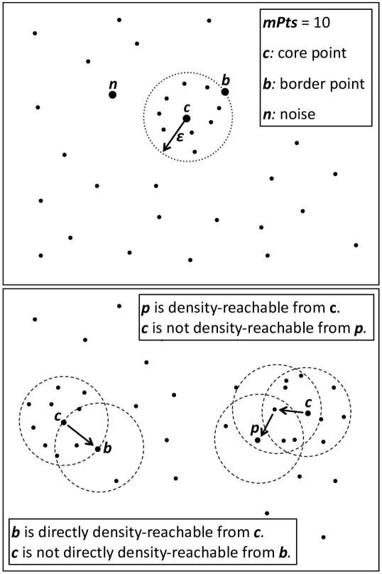
Figure 3: Fundamental concepts used by DBSCAN and OPTICS.

3.2 DBSCAN

The DBSCAN code is one of the most widely used density-based clustering algorithms. Originally introduced by Ester et al. (1996), this algorithm relies on the $\epsilon$ and mPts hyperparameters to find arbitrarily shaped clusters of constant density. The algorithm results strongly depend on these input parameters and the user may have to select the mPts and $\epsilon$ using a trial and error approach.

We begin with the qualitative approach proposed by Ester et al. (1996) to identify optimal mPts and $\epsilon$ values to find clusters in the data. Their method consists in inspecting by eye the so-called sorted $k$-distance plot, which shows the distance to the $k^{th}$ nearest neighbour (the $k$-distance) for each point with all the points sorted out by decreasing $k$-distance. By construction, the points that belong to a cluster containing $k$ members have a lower distance to their closest $k$-neighbours than the noise points. Therefore, a compact cluster containing $n\geq k$ points creates an abrupt decrement in its sorted $k$-distance plot. The $k$-distance at which the curve reduces again its slope corresponds to the optimal $\epsilon$ to identify a cluster using mPts $=k$. This way, examining these curves for different $k$ values allows us to identify pairs of $\epsilon$ and mPts hyperparameters.

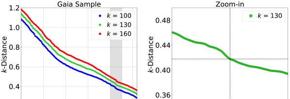
Figure 4: Left: $k$-distance plots of the Gaia sample for different $k$ (or equivalently mPts) values. The grey rectangle encompasses the step-like slope change in the curves (see text). Right: Zoom-in of the $k=130$ case with the bottom of the step-like slope change indicated by the dashed lines.

We generated a set of $k$-distance curves for $k$ ranging between $[80:200]$. A careful look reveals an step-like slope change located at point $\sim 2065$ for $k$ values ranging between $[100:160]$, as indicated by the grey shaded region in the left panel of Fig. 4. To find the appropriate $\epsilon$ values for the different $k$ values (and equivalently, for different mPts) we computed the first and second order derivatives of the sorted $k$-distance curves. Given the density distribution of our dataset we had to resample and smooth the $k$-distance curves with a Gaussian kernel to isolate the $2^{nd}$-order derivative maxima with sampling and smoothing values varying with mPts. After finding the pairs of $\epsilon$ and mPts values for different mPts we run DBSCAN. The algorithm identifies one single cluster dominated by a population of stars with astrometric distributions consistent with those of our control sample. The results of this exploration for three representative cases and their corresponding histogram distributions in parallaxes and proper motions are listed in Table 2 and presented in Fig. 6 (top row), respectively. The histograms in $\,\mu_{\alpha^{*}}$ show a secondary peak at $\,\mu_{\alpha^{*}}$ $\sim-12.5$, which becomes increasingly significant with mPts. A similar behaviour is observed in the $\,\mu_{\delta}$ distribution, which shows a secondary peak at $\,\mu_{\delta}$ $\sim-23$ and is most evident for mPts $=100$. The number of cluster elements varies by $\leavevmode\nobreak\ \sim 10\%$ within the explored range.

3.3 OPTICS

By construction, all the clusters found by DBSCAN in a given dataset have roughly the same density. Furthermore, this algorithm struggles to identify all the members in clusters with strong density gradients, such as a cluster composed of a very dense core surrounded by a low density “halo”. The hierarchical clustering algorithm OPTICS (Ankerst et al. 1999) attempts to overcome these issues by focussing on the density-based clustering structure of the data. The OPTICS algorithm constructs clusters of different densities by exploring a range of $\epsilon$ values and working like an expanded version of DBSCAN.

As a first step, OPTICS finds the densest regions of the cluster and stores this information into two variables named core distance and reachability distance. The former is the distance from a core point to its closest $mPts^{th}$ neighbour, and the latter is the smallest distance that makes a point density-reachable from a core point. For a given value of mPts OPTICS classifies the points according to their reachability distance from the densest part of the cluster. This is reflected in the so-called reachability plot, which shows a series of characteristic valleys, each associated with a potential cluster. The bottom of the valley corresponds to the densest cluster region and the width of the valley roughly scales with the number of cluster elements. The shape of the valley depends on the density distribution of the cluster and the entire dataset. As a second step, OPTICS is executed with the mPts and $\epsilon$ hyperparameters derived from the reachability curves as explained below.

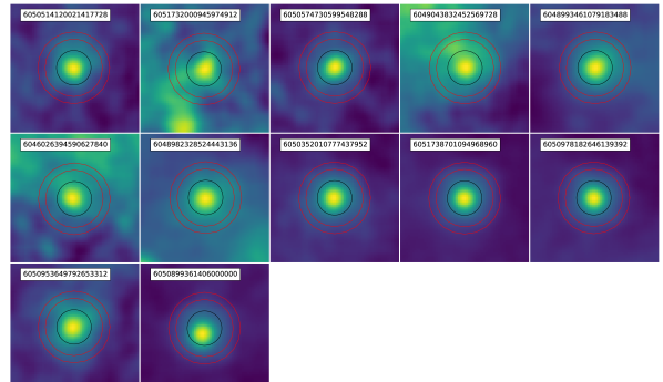
Figure 17: WISE W4 maps of the 12 new discs shown in Fig. 12. The black line encompasses the aperture mask used to find the emission peak associated with the disc ($r=12\arcsec$), and the red lines indicate the ring area used to estimate the background emission ($r_{in}=20\arcsec$, $r_{out}=25\arcsec$; see Sect. 4.3). All the images are $1.5\arcmin\times 1.5\arcmin$ in size, and the white panels indicate the Gaia DR2 source ID.

Following Ankerst et al. (1999) we explored the reachability curves for mPts ranging between $[10:20]$. All the curves show a wealth of substructure in the form of multiple local narrow valleys that smoothly disappear with increasing mPts. The curves also show a main and a secondary (less pronounced) valley (Fig. 5, left panel). We did a first exploration of the two clusters associated with these valleys (see below). The secondary valley is produced by a cluster with $\sim 180$ elements and has averages $\,\varpi$ $=6.3\pm 0.2$, $\,\mu_{\alpha^{*}}$ $=-10.6\pm 1.2$, and $\,\mu_{\delta}$ $=-21.4\pm 1.4$. Its members are part of Cluster 2 shown in Fig. 2 and only one of the control sample members is part of this cluster. On average, the astrometric properties of this secondary cluster are different from those of the control sample and, at first sight, they are consistent with a population of USco stars located in the background of our control sample. We defer a detailed analysis of this cluster to a separate and dedicated study. In what follows we focus our discussion on the main valley and its associated cluster, as this one has astrometric properties similar to those of the control sample. In the explored range the shape of the valley is similar to the “case B” described by Ankerst et al. (1999) in their Sect. 4.3 (see also their Figs. 17 and 18). The valley shows a local plateau at its beginning (labelled as starting of the cluster; SoC), which has similar y-coordinates as the cluster end; this end appears as an abrupt decrement in the curve and is labelled as reachability end (Reach End in the right panel of Fig. 5). In this case, the appropriate $\epsilon$ to extract the cluster for mPts $=16$ corresponds to the $y-$coordinates of the reachability end, that is, $\epsilon$ $=0.259$. The beginning and end of the main valley are clearly detected for mPts ranging between $[14:18]$, and therefore we restrict our analysis to this range. This way we derived the $\epsilon$ values for the corresponding mPts and then executed OPTICS using these hyperparameters. As representative cases we consider those in which the reachability end is clearly detected. Those are listed in Table 2, and their corresponding histograms in parallax and proper motions are shown in Fig. 6 (central row). All the cases produce a similar outcome with a variation in cluster elements $<10\%$. The histogram distributions show a secondary peak at $\,\mu_{\alpha^{*}}$ $\sim-12.5$ and $\,\mu_{\delta}$ $\sim-23$.

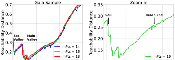
Figure 5: Left: Reachability distance plots of the Gaia sample computed for a range of mPts. Right: Zoom-in of the mPts $=16$ case, highlighting the location of the first and last points of the main valley.

3.4 HDBSCAN

A drawback of both DBSCAN and OPTICS is the potential difficulty in finding optimal $\epsilon$ and mPts values. In high-density datasets it can be complicated to identify unambiguously the step-like slope change in the $k$-distance curves used by DBSCAN and the first and last points of the valleys in the reachability-distance plots generated by OPTICS. The hierarchical algorithm HDBSCAN (Campello et al. 2013, 2015) requires one single hyperparameter to operate (the “minimum cluster size” mCls, conceptually similar to mPts), and it therefore simplifies the task of finding appropriate hyperparameters. Similar to OPTICS, HDBSCAN can identify clusters with different densities and it is sensitive to the density gradients inside a cluster.

The HDBSCAN algorithm is much more complex than DBSCAN and OPTICS and therefore we briefly describe its main steps, referring to Campello et al. (2015) for a thorough description of the algorithm. First, the low-density and noise points are identified by computing the “mutual reachability distance”. This quantity is the maximum of three distances for each pair of data points $A$ and $B$: the core distance to the $k^{th}$ point for $A$ and $B$, and the metric distance between $A$ and $B$. Second, HDBSCAN uses the mutual reachability distance to identify and classify the densest points of the dataset according to their relative density. The points are grouped into clusters through a multi-stage process that involves generating the minimum spanning tree of the mutual reachability distances, computing the data points density hierarchy, and creating a hierarchical condensed cluster tree. Apart from identifying the clusters in a given dataset, HDBSCAN uses the condensed cluster tree to assign a membership probability to each member of a cluster.

We set the probability threshold to the maximum, i.e. we only considered cluster members with $100\%$ associated membership probability, and we then explored the range of mCls values from $[20:100]$. For mCls $>58$ HDBSCAN does not find any cluster, while for mCls between $[20:58]$ the algorithm systematically identifies a main and secondary cluster. After a first exploration we find that the secondary cluster has between 30 and 50 elements, none of which are included in the control sample. As with OPTICS, the members of this secondary cluster have proper motions consistent with those of Cluster 2 in Fig. 2 (with averages $\,\varpi$ $=6.3\pm 0.1$, $\,\mu_{\alpha^{*}}$ $=-10.7\pm 0.9$, and $\,\mu_{\delta}$ $=-21.3\pm 1.3$). As explained before, in this paper we focus our attention on the main cluster found by HDBSCAN because its astrometric properties are consistent with those of the control sample. For mCls ranging from $[20:58]$ the number of cluster members mostly oscillates around $\leavevmode\nobreak\ 460$. As representative outputs we consider those listed in Table 2 as, excluding a few cases with number of elements $<200$, those encompass the minimum, maximum, and roughly average number of elements of the main cluster. The corresponding histograms are shown in Fig. 6 (bottom row). The proper motion distributions show two secondary peaks at $\sim-12.5$ in $\,\mu_{\alpha^{*}}$ and $\sim-23$ in $\,\mu_{\delta}$, albeit these peaks are less pronounced than in the DBSCAN and OPTICS cases.

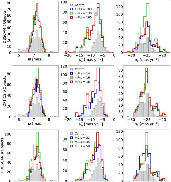
Figure 6: Histogram distributions of the cluster identified by DBSCAN (top) and the main cluster identified by OPTICS (centre) and HDBSCAN (bottom) for different hyperparameters (see legend and Table 2). The control sample is represented with grey bars.

Algorithm	mPts	Eps	Elements	Control (%)
DBSCAN	100	0.373	492	155 (82.4)
DBSCAN	130	0.418	524	156 (83.0)
DBSCAN	160	0.455	552	158 (84.0)
OPTICS	14	0.245	451	157 (83.5)
OPTICS	16	0.259	494	157 (83.5)
OPTICS	18	0.265	497	159 (84.6)
HDBSCAN	21	–	427	153 (81.4)
HDBSCAN	35	–	502	163 (86.7)
HDBSCAN	50	–	462	158 (84.0)

Table 2: Explored hyperparameters and number of cluster elements identified by each algorithm. The fifth column indicates the number of control sample members found; the percentage is indicated inside a parenthesis. For HDBSCAN the first column corresponds to the mCls.

3.5 Common sample

The three algorithms previously discussed find a population of objects with astrometric properties (excluding the yet unknown radial velocity) consistent with those of the control sample, and additionally OPTICS and HDBSCAN find a secondary cluster with different average properties. As explained in Sect. 3.3, the fact that DBSCAN does not find this smaller cluster probably reflects one of the main weaknesses of this algorithm, which is its lack of sensitivity to find clusters with different densities in the same dataset. Regarding the main cluster of our sample, the algorithm outputs are slightly different and the cluster size is sensitive to the chosen algorithm and corresponding hyperparameters (see Table 2). On average, each algorithm recovers roughly 84% of the control sample. It is therefore not straightforward to decide which algorithm and hyperparameter combination produces the most reliable sample of potential $\rho$ Oph members. To overcome this difficulty we merged the results listed in Table 2, conservatively choosing the cluster combination that produces the smaller output in terms of elements. That is, we combined the DBSCAN output obtained for mPts $=100$, the OPTICS output with mPts $=14$, and the HDBSCAN output with mCls $=21$. After accounting for duplicates the merged cluster (labelled hereafter as combined sample) contains 532 sources, 164 of which are included in the control sample. In this cluster there are 59 sources only detected by DBSCAN, and 13 sources only detected by OPTICS and other 13 only by HDBSCAN. Table 3 lists the members of this sample and includes a column labelled as ”DOH” (acronym for DBSCAN-OPTICS-HDBSCAN), which indicates the algorithm(s) that detect each member using a ”Y/N” nomenclature. For example, if a source is detected only by DBSCAN its DOH value is ”YNN”, while the DOH value of a member detected by OPTICS and HDBSCAN has is ”NYY”. From this combined sample we extracted the sources simultaneously identified by the three algorithms (i.e. those with DOH$=$”YYY”). Hereafter we focus our analysis on this common sample that contains 391 sources, 148 of which belong to the control sample.

$\,\alpha$	$\,\delta$	$\,\varpi$	$\,\mu_{\alpha^{*}}$	$\,\mu_{\delta}$	source_id	Control	DOH
$[\mathrm{deg}]$	$[\mathrm{deg}]$	$[\mathrm{mas}]$	[mas yr ${}^{-1}]$	[mas yr${}^{-1}]$
243.3719939	-23.1855471	7.2072955	-8.8893582	-25.4157242	6242554649124043520	N	YNN
243.7959809	-23.3786153	7.1327026	-15.5389965	-24.4785008	6050385511522948096	N	YNN
243.8016470	-23.3127069	7.1572953	-8.8631422	-26.3450177	6050388913137070848	N	YNY
243.8311704	-25.6701140	7.4134597	-9.1980374	-27.1873024	6048740710844628864	N	YNN
243.8642421	-22.6577711	7.1951507	-10.8897003	-24.8620069	6242599763466335104	N	YNY

Table 3: First 5 entries of the combined sample (532 members) described in Sect. 3.5. The sixth column is Gaia DR2 source_id. The entire table is provided in the electronic version of this article. The control column indicates if a target is part of the control sample following a Yes/No nomenclature. All the coordinates are given in J2015.5 epoch (as in Gaia DR2).

The common sample contains 243 potential Ophiuchus member candidates that were not included in the three catalogues used to construct the control sample described in Sect. 2.2. In order to gather further information about these sources, we queried the SIMBAD database using as identifier the Gaia DR2 source_id. This query returned 77 objects, that is, to date 166 objects in our common sample do not appear linked to any publication according to the SIMBAD service. Combining the results obtained by Kraus & Hillenbrand (2007), Luhman & Mamajek (2012), and Rizzuto et al. (2015), we find that 43 targets out of the 77 known objects have been associated with the USco subgroup of the Scorpius-Centaurus OB association.

4 Results

4.1 Astrometric properties

The sky-projected distribution of the common sample is shown in Fig. 7 superimposed on the extinction map produced by the COMPLETE project (Ridge et al. 2006) applying the NICER algorithm (Lombardi & Alves 2001) to 2MASS observations. Nearly one-third of the common sample objects (125 sources) are found within a distance $r\leq 0.6\degr$ from the extinction peak (roughly at $\alpha,\delta=246.7\degr,-24.5\degr$) of the main dark cloud of Ophiuchus, the Lynds 1688 dark cloud (L1688; see e.g. Wilking et al. 2008). Most of these objects (113) are also included in the control sample. The apparent lack of sources at the innermost core of this cloud is most likely a consequence of the very high extinction exceeding $A_{\mathrm{V}}>20$ at this location. We do not find a significant correlation between the distances to each object (indicated by the rainbow colour bar) and the sky-projected location of the sample.

Figure 8 shows the proper motions of the common sample (plotted as small cyan circles) overlaid on the zoomed-in distributions of the Gaia sample (as grey circles). As in Fig. 2, the diameter of the grey circles equals the average error on $\,\mu_{\alpha^{*}}$ of the Gaia sample. The 40 control sample sources not included in the common sample are plotted as small magenta circles. Most of the common sample members are concentrated around the apparent cluster located at higher $\,\mu_{\alpha^{*}}$ values (Cluster 1 in Fig. 2), but a non-negligible fraction of these members are also found in the apparent cluster located towards lower $\,\mu_{\alpha^{*}}$ and higher $\,\mu_{\delta}$ values (Cluster 2 in Fig. 2). The parallax and proper motion histograms of the common sample are shown in Fig 9. The three distributions deviate from a single bell-shaped distribution and the parallax histogram shows two separate peaks at $\varpi=7.0$ and $\varpi=7.2$. The parallax distribution is narrower than the control sample counterpart ($\,\varpi$ $\in[6.7:7.7]$ versus $\,\varpi$ $\in[5.7:8.5]$). By computing the distance as the inverse of the parallax, we obtain an average distance of $d=139.4_{-3.8}^{+4.1}$ pc to the common sample. The difference in parallax ranges means that the common sample members are distributed in a localised spatial region with distances ranging from $[130:150]$ pc, whereas the control sample occupies a spatial region with distances ranging between $[118:176]$ pc. The proper motion histograms show a secondary peak or shoulder at $\,\mu_{\alpha^{*}}$ $\sim-12$ and $\,\mu_{\delta}$ $\sim-21$, as expected from Fig. 8. We fitted a combination of two Gaussian profiles to the $\,\mu_{\alpha^{*}}$ and $\,\mu_{\delta}$ distributions using a Levenberg-Marquardt algorithm; the fit did not converge for the parallax distribution. The fits are shown as a solid (combined fit), dashed (main Gaussian), and dotted (secondary Gaussian) lines overlaid on the histograms in Fig. 9. The mean and full width at half maximum (FWHM) of the Gaussian fits and the average astrometric properties of the common sample are listed on Tables 4 and  5, respectively.

It is likely that our common sample contains members of the USco region given the similarity between the proper motions of USco and $\rho$ Oph, the proximity between these two regions, and the large extension of USco across the sky (e.g. Mamajek 2008; Preibisch et al. 2002; Preibisch & Mamajek 2008). We used the USco control sample with trigonometric parallaxes discussed by Galli et al. (2018) to compare the astrometric properties of both samples. The average parallax and proper motions of the USco sample ($\,\varpi$ $=7.1\pm 0.5$, $\,\mu_{\alpha^{*}}$ $=-11.7\pm 3.1$, and $\,\mu_{\delta}$ $=-23.9\pm 1.9$) are indicated by the blue vertical dot-dashed lines in Fig. 9. The average $\,\mu_{\alpha^{*}}$ of the USco sample coincides with the secondary peak of the $\,\mu_{\alpha^{*}}$ histogram distribution of our common sample, which we attribute to the presence of USco stars in our sample.

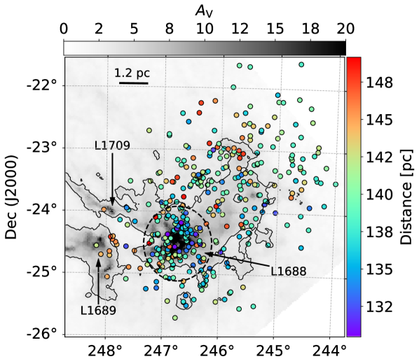
Figure 7: Common sample overlaid on top of an extinction map. The contour delimits the $A_{\mathrm{v}}=4$ regions. The arrows indicate the location of the main Lynds dark clouds in this area, while the black dashed line encompasses the $r\leq 0.6\degr$ region centred on the extinction peak. The size scale is calibrated for the average distance to the common sample.

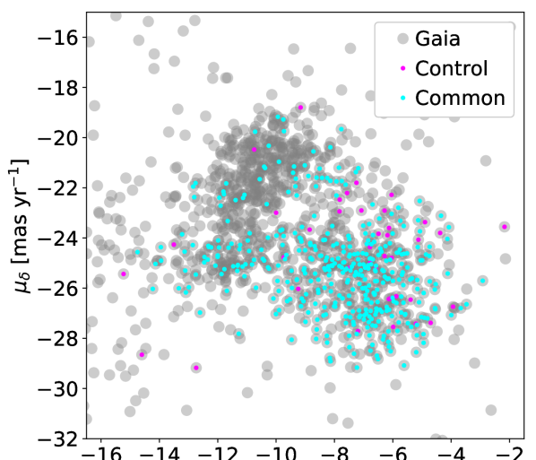
Figure 8: Same as Fig. 2, including the common sample as cyan small circles. The 40 sources from the control sample not included in the common sample are shown as small magenta circles.

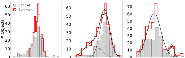
Figure 9: Histogram distributions of the common sample (see Sect. 3.5). A two-Gaussian fit is shown as a solid line superimposed on the proper motion histograms.

	$\,\mu_{\alpha^{*}}$	$\,\mu_{\delta}$
	$[$mas yr${}^{-1}]$	$[$mas yr${}^{-1}]$
Mean	$-6.9\pm 0.1$	$-25.4\pm 0.1$
FWHM	$3.2\pm 0.1$	$3.4\pm 0.1$
Mean	$-10.4\pm 0.5$	$-21.6\pm 0.1$
FWHM	$4.8\pm 0.8$	$1.0\pm 0.4$

Table 4: Mean and FWHM of the Gaussian fits shown in Fig. 9 for the main and secondary Gaussians (upper and lower halves, respectively). The errors are the $1\sigma$ uncertainties of the fit.

Dimension	Value
$\,\alpha$	$246.2^{\circ}\pm 0.8$
$\,\delta$	$23.9^{\circ}\pm 0.8$
$\,\varpi$	$7.2\pm 0.2$ mas
$\,\mu_{\alpha^{*}}$	$-8.0\pm 2.2$ mas yr-1
$\,\mu_{\delta}$	$-25.2\pm 1.9$ mas yr-1
$X$	$132.1\pm 3.8$ pc
$Y$	$-15.8\pm 1.4$ pc
$Z$	$41.9\pm 2.6$ pc

Table 5: Mean and standard deviation ($1\sigma$) of the common sample across different dimensions. The Cartesian coordinates are given in the Galactic reference frame ($X$, $Y$, and $Z$ point towards the Galactic centre, the direction of the Galactic rotation, and the North Galactic Pole, respectively).

4.2 Colour magnitude diagram

Fundamental properties like stellar masses or ages can be estimated from a colour magnitude diagram (CMD), if the extinction for each object is known. There are photometric measurements for all the objects in our common sample in the three Gaia bands (broad $G$ and the two narrower $G_{\mathrm{BP}}$ and $G_{\mathrm{RP}}$; Brown et al. 2018) bands, but the extinction is estimated for only 95 of these objects and has an average value of $\,A_{\mathrm{G}}$ $=1.7\pm 0.6$. As noted by Andrae et al. (2018) the Gaia extinctions are not accurate at the individual star level. Most importantly for our particular case, the effective temperatures and extinctions listed on the Gaia DR2 are based on a naked stellar model that does not include the contribution from the dust in the SFR or the protoplanetary discs that probably surround an important fraction of the common sample sources. Therefore we looked for published extinction values of our sources. Dunham et al. (2015) gave extinction values in the $V$ band, $\,A_{\mathrm{V}}$, for 83 objects with an average value of $\,A_{\mathrm{V}}$ $=6.0\pm 4.0$. Rizzuto et al. (2015) estimated $\,A_{\mathrm{V}}$ for another 20 objects with an average value of $\,A_{\mathrm{V}}$ $=0.9\pm 0.6$. The large difference between both studies is because, by construction, the sample by Dunham et al. (2015) is composed of YSOs surrounded by discs, while the sample discussed by Rizzuto et al. (2015) is dominated by objects without detected discs. Combining both studies we obtain $\,A_{\mathrm{V}}$ estimates for $26\%$ of the sources in the common sample that have an average extinction of $\,A_{\mathrm{V}}$ $=5.0\pm 4.1$. Using the Gaia DR2 extinction coefficients listed in the filter profile service provided by the Spanish Virtual Observatory (SVO; Rodrigo et al. 2012) this average value translates into $\,A_{\mathrm{G}}$ $=4.7$. As the individual extinctions for most of the sources remain unknown to date, we opted for constructing an extinction uncorrected CMD. For this purpose we used the $G$ and $G_{\mathrm{RP}}$ bands, as their characteristic error is lower than in the $G_{\mathrm{BP}}$ band; for our entire sample we obtain a $\delta G,\delta G_{\mathrm{RP}}$, and $\delta G_{\mathrm{BP}}$ of $0.002,0.007$, and $0.04$ mags, respectively. We used the individual parallaxes to compute the absolute magnitudes for each source as $M=m+5(\log_{10}\varpi+1)$. We computed the extinction vector using the previously mentioned average $\,A_{\mathrm{G}}$ to get a rough idea of the extinction effect. Figure 10 shows the obtained diagram; the common sample is plotted as small cyan circles superimposed on the grey circles that represent the Gaia sample. As in Fig. 8, the 40 sources that belong to the control sample but not included in the common sample are shown as magenta small circles. Except for a few objects, the common sample occupies a separate region in this plot, as expected if this sample is significantly younger than the rest of the stars in the Gaia sample. Given the high extinction of the $\rho$ Oph region the common sample is most likely composed of objects located in the near side of the cloud surface, as those in the inner regions of the cloud are probably too obscured to be detected by Gaia. Median ages for $\rho$ Oph members at the cloud surface range from 2 Myr to 5 Myr (Wilking et al. 2008). To put our sample in context we gathered the BT-Settl/CIFIST (Baraffe et al. 2015) and Parsec (Marigo et al. 2017) stellar evolutionary models for stellar masses below and above $1.4\,M_{\odot}$, respectively. The 2 and 5 Myr isochrones drawn from these models are shown as a solid and a dashed blue line overlaid on the CMD, respectively, while the evolutionary tracks for three different stellar masses ($0.1,0.5$, and $1.4\,M_{\odot}$) are indicated by orange thick lines. Most of the common sample objects are located above the isochrone. Similarly, the bulk of the common sample ($\sim 90\%$ of it) lies below the $0.5\,M_{\sun}$ evolutionary track.

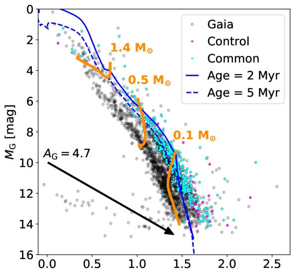
Figure 10: Colour magnitude diagram. The control sample sources not included in the common sample are shown as small magenta circles. The diameter of the black circles is larger than the average photometric error. The extinction vector is computed for the average $\,A_{\mathrm{G}}$ derived from a subset of sources (see Sect. 4.2).

4.3 Potential discs

Given the youth of $\rho$ Oph, a large fraction of our common sample members might be surrounded by protoplanetary discs. The presence of such a disc, as well as its evolutionary stage, can be inferred from the warm dust emission at infrared wavelengths. We used the crossmatched tables provided by the Gaia consortium (available in the Gaia archive) gaiadr1.tmass_original_valid and gaiadr2.tmass_best_neighbour to obtain the near-infrared photometry for the common sample sources. By combining these two tables we retrieved the 2MASS photometry for 382 sources. We then repeated the same procedure but using the gaiadr2.allwise_best_neighbour and gaiadr1.allwise_original_valid tables to obtain the mid-infrared photometry measured by the Wide-Field Infrared Survey Explorer (WISE; Wright et al. 2010), retrieving observations for 332 sources. All the retrieved 2MASS photometry has quality flag ”A” at the three bands, but this is not the case for the WISE photometry. Therefore, before combining these outputs we disregarded the objects with photometric quality flags different than ”A” or ”B” at any of the WISE bands. Furthermore, we only considered objects with contamination and confusion flags (cff) equal to ”0” in all WISE bands, and with extended source flags (ex) lower than 2. At this stage, we inspected by eye the WISE images of every source to remove those affected by artefacts. The WISE band 4 photometry can be strongly affected by background emission, which might be mistakenly associated with the warm dust emission produced by a circumstellar disc (Kennedy & Wyatt 2012). To minimise this potential confusion we used the Astropy/photutils package to perform aperture photometry to measure the signal to noise at the peak of the WISE band 4 image of each source. We used an aperture mask with radius $r_{\mathrm{ap}}=12\arcsec$ to measure the peak emission and a sky aperture ring of $r_{\mathrm{in}}=20\arcsec$ and $r_{\mathrm{out}}=25\arcsec$ to estimate the background signal; both apertures were centred on the Gaia DR2 coordinates ($\,\alpha$ and $\,\delta$) for each source. We filtered out all the sources with peak emission S/N $\leq 4$. Applying this selection criteria we finally obtained a sample of 48 sources, of which 25 belong to the control sample, with 2MASS and WISE photometry.

We combined the Gaia photometry with the infrared photometry to build up the spectral energy distributions (SEDs) for the 48 sources previously selected. To convert from magnitudes to flux units (Jy) we retrieved the effective wavelengths and zero points (ZP) for each photometric band from the SVO. The total uncertainty of the fluxes was computed as the quadratic sum of the errors associated with the photometric extraction process, ZP, and systematic errors. The Gaia photometric uncertainties are negligible compared to those from the 2MASS and WISE. The largest source of uncertainties are the systematic errors associated with the WISE photometry, which is tied to the Spitzer photometric calibration (Jarrett et al. 2011). In this work we adopt an absolute calibration uncertainty of 5% for the W1, W2, and W3 bands, and 10% for the W4 band. Given the broad wavelength coverage of the WISE filters, a colour correction must be applied when transforming magnitudes to fluxes. For each source we computed the $\alpha$ flux slope ($F_{\nu}\sim\nu^{\alpha}$) for the different WISE bands and then applied the correction factors following Section VI of the Explanatory Supplement to the WISE All-Sky Data Release Products.

Traditionally, the protoplanetary discs have been classified according to the infrared slope of their SED defined as

$$\alpha_{\mathrm{IR}}={\frac{log(\lambda_{1}F_{\lambda_{1}})-log(\lambda_{0}F_{\lambda_{0}})}{log(\lambda_{1})-log(\lambda_{0})}},$$ (4)

where $\lambda_{1}$ and $\lambda_{0}$ correspond to $\sim$2 and $\sim$22  $\mu\mathrm{m}$ (Lada & Wilking 1984; Lada 1987). This way, objects with $\,\alpha_{\mathrm{IR}}$ $>0.3$ (i.e. those with an increasing SED towards the mid-infrared) are labelled as Class I and are associated with YSOs surrounded by a primordial envelope and massive, little evolved disc. Objects with $-0.3>$$\,\alpha_{\mathrm{IR}}$ $>-1.6$ are classified as Class II sources and represent a more evolved stage during the disc evolution, while those with $0.3>$$\,\alpha_{\mathrm{IR}}$ $>-0.3$ are classified as flat SED sources and show intermediate properties between the Class I and II stages (Greene et al. 1994). Objects with $\,\alpha_{\mathrm{IR}}$ $<-1.6$ are classified as Class III and they are associated with tenuous discs. Applying this criteria and using the $K_{\mathrm{s}}$ ($\lambda_{\mathrm{eff}}\sim 2.2$ $\mu\mathrm{m}$) and W4 ($\lambda_{\mathrm{eff}}\sim 22.1$ $\mu\mathrm{m}$) bands, we find 36 Class II and 12 Class III objects within the 48 objects with infrared photometry contained in the common sample. This traditional classification is useful and allows for comparison with previous works, but it has some limitations (see e.g. Cieza et al. 2007; Merín et al. 2010). In particular, as already noted by Evans et al. (2009), the Class III encompasses two different types of objects: those surrounded by a tenuous disc, and those with no detectable infrared excess (i.e. bare photospheres). Inspecting the computed SEDs we find several of these objects within the Class III of our sample. Therefore we applied an extra classification based on the infrared slope between $\sim 12$ $\mu\mathrm{m}$ and $\sim 22$ $\mu\mathrm{m}$ ($\alpha_{\mathrm{W34}}$). We classify as bare photospheres the Class III objects with $\alpha_{\mathrm{W34}}<-1.6$, and reclassify the Class III objects as those with $\,\alpha_{\mathrm{IR}}$ $<-1.6$ and $\alpha_{\mathrm{W34}}>-1.6$. Using this classification scheme we identify 7 bare photospheres and 5 Class III sources, as reflected in Fig. 11. Therefore, we find a disc fraction of $\sim 85\%$ in this subsample of 48 objects. Bearing in mind the strong selection biases of our sample, we note that this high disc fraction is consistent with an age of $\sim 2$ Myr according to different studies (e.g. Ribas et al. 2015; Fedele et al. 2010; Mamajek 2009). A table with the photometry for these 48 objects is given in the Appendix (Table 9) and is available in the electronic version of this article. This table contains a “status” keyword that indicates if a disc is included in the control sample (labelled as control), or if the disc has currently no references in the SIMBAD service (labelled as new). We find 12 new discs, 11 of which have Class II SEDs and 1 of which have Class III SED (Gaia DR2 $\#$6051732000945974912). The SEDs for these 12 new discs are shown in Fig. 12, and their corresponding WISE W4 images are shown in the Appendix (Fig. 17). We note that the disc around the Gaia DR2 $\#6050899361406000000$ source shows a strong increase towards 22 $\mu\mathrm{m}$ characteristic of a disc with a large dust depleted inner cavity as in for example Sz 91 (Canovas et al. 2015, 2016; Tsukagoshi et al. 2014).

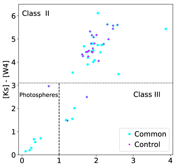
Figure 11: Colour-colour plot of the common sample with high quality infrared photometry. The dotted line indicates the traditional boundary between the Class II and III stages. The vertical dashed line separates bare photospheres from Class III discs.

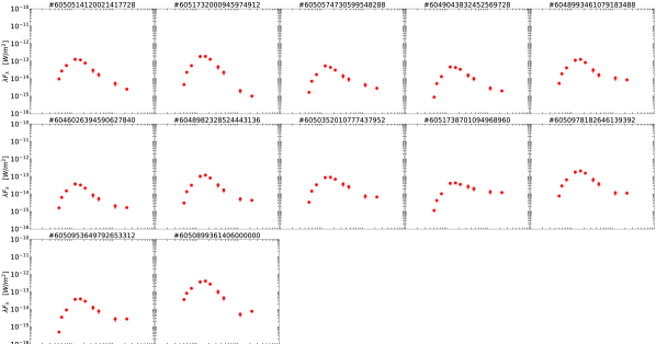
Figure 12: Spectral energy distributions of the 12 new discs detected. The title indicates their Gaia DR2 source ID. The panels are ordered by increasing $\alpha_{W34}$ slope. Object $\#6051732000945974912$ is the only Class III disc of this subsample, as the rest are Class II discs. Source $\#6050899361406000000$ shows the characteristic SED shape of a disc with a dust depleted inner cavity.

5 Summary and conclusions

In this work we have used three density-based clustering algorithms (DBSCAN, OPTICS, and HDBSCAN) to identify potential new members of the $\rho$ Oph region in the Gaia DR2 catalogue. The members of the same SFR have similar proper motions and spatial distributions, so these ML algorithms are well suited to detect new member candidates.

We began by constructing a comprehensive sample of Ophiuchus members previously identified by Wilking et al. (2008), Erickson et al. (2011), and Dunham et al. (2015). Table. 6 lists the 465 elements of this catalogue. We then used the 2MASS source IDs of these objects to cross-match them against the Gaia DR2 catalogue. We obtained a control sample composed of 188 elements by applying the quality selection criteria described in Sect. 2.2 and removing the outliers. This catalogue of bona fide members, which may be useful for future studies of the $\rho$ Oph cloud, is accessible via Table. 6 through the Control keyword. We then downloaded the Gaia DR2 sources contained within a circular area of $r=3.5\degr$ centred on $\rho$ Oph and with $5<$$\,\varpi$ $<9$, a region large enough to encompass the entire control sample (Fig. 1). We imposed the quality selection criteria outlined in Sects. 2.2 and  2.3, and then separately applied the DBSCAN, OPTICS, and HDBSCAN algorithms to the five astrometric dimensions ($XYZ$ Cartesian coordinates and the proper motions $\,\mu_{\alpha^{*}}$ and $\,\mu_{\delta}$) of this sample. The DBSCAN code systematically finds one large cluster consistent with the control sample astrometric properties, while OPTICS and HDBSCAN identify two clusters, the largest of which has astrometric properties similar to those of the control sample (Fig. 6). Discussing in detail the properties of the secondary cluster is out of the scope of this paper, and we defer its analysis to a separate study. The size of the main cluster depends on the algorithm hyperparameters, ranging from 427 to 552 elements. On average, the algorithms recover $\sim 84\%$ of the control sample as shown in Table 2. By combining the different algorithm outcomes we constructed the minimum common sample. This sample, presented in Table 3, contains 391 candidate members of $\rho$ Oph including 148 control sample elements and 166 sources that, to date, have no reference in the literature according to SIMBAD. Seventy-seven sources appear associated either with $\rho$ Oph or USco (i.e. Cieza et al. 2007; Cheetham et al. 2015; Luhman & Mamajek 2012; Rizzuto et al. 2015). The average distance to the common sample ($d=139.4_{-3.8}^{+4.1}$ pc) is consistent, within error bars, with previous distance estimates towards the $\rho$ Oph cloud (Makarov 2007; Mamajek 2008; Ortiz-León et al. 2017, 2018).

In Sect. 4.1 we analysed the astrometric properties of the common sample. The parallax distribution is narrower than that of the control sample, ranging from $[6.7:7.7]$ and showing a double peak at $\,\varpi$ $=7.0,7.2$. The proper motion histograms show double Gaussian-like profiles with main and secondary peaks at $-6.9\pm 0.1$ and $-10.4\pm 0.5$ in $\,\mu_{\alpha^{*}}$, and $-25.4\pm 0.1$ and $-21.6\pm 0.1$ in $\,\mu_{\delta}$ (Figs. 8 and  9, and Table 4). The extinction uncorrected CMD is shown in Fig. 10 and discussed in Sect. 4.2. The CMD suggests that the common sample is dominated by objects younger than 5 Myr with masses below $0.5\,M_{\sun}$, which agrees with previous studies of this cloud (Wilking et al. 2005; Erickson et al. 2011), but we are cautious about our conclusions given the large uncertainty associated with the (yet unknown) extinction of these sources. Finally, in Sect. 4.3 we constructed the SEDs from optical to mid-infrared wavelengths for the subset of 48 objects with high quality photometry in the Gaia, 2MASS, and WISE bands. We identified 36 Class II, 5 Class III objects, and 7 bare photospheres by applying a colour selection criteria (Fig. 11). Their photometry, along with their SED Class and a flag indicating if the object has no references in SIMBAD, is given in Table. 9. Twelve of these objects have no references on the SIMBAD service and show strong infrared emission, and their SEDs are shown in Fig. 12. Their corresponding WISE W4 maps are presented in Fig 17.

This work reflects the potential of applying modern ML techniques to identify young stellar populations in huge astronomical catalogues such as the Gaia DR2. Our results show that the DBSCAN, OPTICS, and HDBSCAN algorithms identify a similar population of potential members of the $\rho$ Oph SFR. All of these algorithms recover roughly 84% of the control sample and the number of elements of the main cluster found does not present strong variations when comparing the different algorithm outputs. The lack of a complete census of bonafide members of $\rho$ Oph prevents us from performing a quantitative analysis to decide which algorithm is the more adequate to find potential member candidates in this cloud. We therefore choose to focus our analysis in the minimum-sized common sample composed of the cluster elements simultaneously found by the three algorithms. This common sample contains fewer elements than the clusters identified by each method separately (391 members versus, e.g. 427 for HDBSCAN with mPts = 21; see Table 2), so it is possible that because of our rather conservative approach we are missing potential cluster members. Nevertheless, the entire list of candidate members found by the three algorithms is given in Table 3 with the hope that this sample will be useful for future studies by the community.

We are cautious about the possible generalisation of our analysis to other SFRs or stellar associations. While some regions have a very compact spatial distribution (e.g. IC 348, Ruíz-Rodríguez et al. 2018, and references therein), others are distributed across several parsecs (e.g. USco, Galli et al. 2018; Preibisch & Mamajek 2008), and furthermore some present a rich and complex spatial substructure (like Taurus, Joncour et al. 2018). Therefore it is possible that the agreement in the outputs produced by DBSCAN, OPTICS, and HDBSCAN when analysing $\rho$ Oph is not reached when analysing other regions with different geometry and dynamics.

These tools are especially useful when the region under study is affected by a high extinction that hinders a sample selection from a CMD (as in e.g. Goldman et al. 2018). However, we are aware of a number of limitations of our study. To begin with, none of the algorithms discussed in this work take into account the measurement uncertainties and, as shown through our analysis, the outcomes are sensitive to the hyperparameters given by the user. We attempted to overcome these issues by combining the results of the three algorithms and focussing our analysis on the minimum size common sample of the multiple cases listed in Table 2. Another caveat to consider is that SFRs are very complex environments and a fraction of their components might not be located in a cloud core but in a stream or filament-like spatial structure (André et al. 2010). This is indeed the case for $\rho$ Oph; at least two prominent filaments seem to departure from the L1688 dark cloud (Ridge et al. 2006). This complex spatial distribution makes it more difficult for the clustering algorithms to identify the cloud members, and that can explain why the applied algorithms recovered $\sim 84\%$ of the sample rather than the entire control sample. This can also explain the narrow range in the parallax distribution of the common sample when compared to that of the control sample. A third important caveat is that, given the proximity in terms of parallax and coordinates, it is possible that a fraction of the stars in our sample was formed in the $\sim 10$ Myr old USco region (Pecaut et al. 2012; Pecaut & Mamajek 2016). The remarkable overlap between the average $\,\mu_{\alpha^{*}}$ of the USco sample discussed by Galli et al. (2018) and the secondary peak found in the $\,\mu_{\alpha^{*}}$ histogram of our common sample, together with the fact that 43 members of the common sample have been associated with USco, is an indicative of this possible contamination. A potential way to discern the nature of these sources would be to analyse the radial velocities, which we have not included in our study given the lack of measurements in the Gaia DR2. Future data releases are expected to include more radial velocity measurements and therefore will become ideal catalogues to repeat studies like this one. In the meantime, the brighter objects of the common sample could be followed up with spectroscopy in order to determine their effective temperatures and extinctions, and therefore to estimate their ages and masses; this would also help to constrain their parental region.

It is not surprising that none of the studied objects with infrared photometry belong to the earlier Class 0 and I stages. These objects are very embedded and extinct, and therefore they are relatively difficult targets for Gaia. The 12 discs that we discovered are good candidates to be directly imaged at optical and near-infrared wavelengths with high-contrast instruments such as SPHERE (Beuzit et al. 2008) at the Very Large Telescopes (VLT), and at submillimeter and longer wavelengths with the ALMA observatory. Given the high fraction of circumstellar discs that we found in our subset of 48 targets ($\sim 85\%$), the objects discussed which lack infrared photometry are promising targets to search for discs with future infrared facilities such as the James Webb Space Telescope (JWST) and proposed missions such as the Space Infrared Telescope for Cosmology and Astrophysics (SPICA).

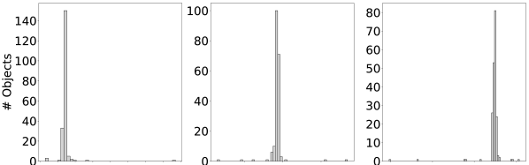
Figure 14: Parallax and proper motion histograms of the astrometrically cleaned sample. We note the few outliers located far away from the histogram peaks.

2MASS	Refs.	Control	DR2 Source ID
16261949-2437275	1, 2, 3	Y	6049122310095142656
16262083-2428395	1, 3	N
16262096-2408468	3	Y	6049357429490158336
16262097-2408518	1, 2	Y	6049357433785068672
16262138-2423040	1, 3	N

Table 6: Extract of the initial sample presented in Sect. 2.1. The entire table is listed in the electronic version of the article. References are coded as 1: Wilking et al. (2008), 2: Erickson et al. (2011), and 3: Dunham et al. (2015). Note: Five targets have duplicate Gaia source_id: 2MASS J16222099-2304025, 2MASS J16233609-2402209, 2MASS J16253958-2426349, 2MASS J16275565-2444509, and 2MASS J16282373-2441412. These duplicates are removed when applying the selection criteria described in Sect. 2.2, but we keep them in the table for consistency.

2MASS ID	$\,\varpi$	$\,\mu_{\alpha^{*}}$	$\,\mu_{\delta}$
	[$\mathrm{mas}$]	[mas yr-1]	[mas yr-1]
16293441-2452292	8.9451	-37.9989	-118.5701
16442882-2412242	2.1726	-1.8833	-5.9312
16245652-2459381	1.4977	-7.6758	-3.7136
16265752-2446060	10.2548	56.4965	-59.1305
16282516-2445009	13.1651	-52.7356	-62.1384
16244802-2440051	38.5067	-85.4146	-152.0051
16260302-2423360	7.4456	-20.1836	-26.7646
16273052-2432347	9.3827	84.3542	-41.9827
16273714-2359330	2.0953	4.7860	4.0732

Table 7: Objects excluded from the control sample. They appear as outliers on the bell-shaped histograms shown in Fig. 14.

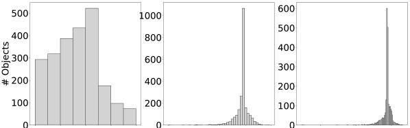
Figure 16: Same as Fig. 14 but for the Gaia cleaned sample.

DR2 Source ID	Ref.	$\,A_{\mathrm{V}}$	$\,A_{\mathrm{G}}$
		$\mathrm{mag}$	$\mathrm{mag}$
6046062364938324608	1	4.2	0.8
6047590243721186688	1	4.4	2.6
6049067776894321024	1	3.9	1.3
6049094616145974272	1	6.3	2.2
6049095406419962112	1	7.9	1.9
6049101866050768384	1	2.9	1.9
6049118388788178816	1	4.0	2.8
6049122310095142656	1	1.6	2.2
6049142410542091648	1	4.5	2.8
6049161514556593920	1	15.9	2.0
6049162545348745984	1	10.8	2.1
6049331526542488064	1	6.6	2.0
6049367398109200256	1	6.3	1.4
6050172068822858624	1	0.0	0.7
6050204641855013376	1	3.9	1.3
6050345001390940160	2	0.6	0.8
6050487456864139392	2	0.9	1.6
6050626201483958400	1	2.0	2.3
6050644102907664640	1	1.9	0.9
6050681211424993280	1	4.3	2.1
6051734990243252096	1	2.2	1.9
6051764573978499200	2	0.8	0.9

Table 8: Objects in the common sample with published $\,A_{\mathrm{V}}$ and Gaia DR2 $\,A_{\mathrm{G}}$ values (see Sect. 4.2). References are coded as (1): Dunham et al. (2015), (2): Rizzuto et al. (2015).

source_id	G_Flux	BP_Flux	RP_Flux	J_Flux	H_Flux	Ks_Flux	W1_Flux	W2_Flux	W3_Flux	W4_Flux	SED_Class	status
	$\mathrm{W\,m^{-2}}$	$\mathrm{W\,m^{-2}}$	$\mathrm{W\,m^{-2}}$	$\mathrm{W\,m^{-2}}$	$\mathrm{W\,m^{-2}}$	$\mathrm{W\,m^{-2}}$	$\mathrm{W\,m^{-2}}$	$\mathrm{W\,m^{-2}}$	$\mathrm{W\,m^{-2}}$	$\mathrm{W\,m^{-2}}$
6046026394590627840	6.38E-15	1.62E-15	1.52E-14	3.75E-14	3.26E-14	2.17E-14	8.44E-15	5.24E-15	2.02E-15	1.68E-15	Class II	New
6047564611356188288	3.76E-15	4.11E-16	1.06E-14	7.34E-14	1.05E-13	8.79E-14	4.43E-14	2.88E-14	7.53E-15	5.38E-15	Class II	Control
6047569834036585728	4.24E-14	1.35E-14	9.17E-14	2.50E-13	2.80E-13	2.02E-13	9.91E-14	7.08E-14	3.23E-14	2.90E-14	Class II	Control
6047573849829430656	4.76E-16	1.25E-16	1.73E-15	2.22E-14	3.37E-14	3.57E-14	2.09E-14	1.64E-14	7.72E-15	5.90E-15	Class II	Control
6047584810585556480	2.84E-13	1.38E-13	5.05E-13	8.85E-13	9.02E-13	5.70E-13	2.10E-13	9.12E-14	6.38E-15	1.19E-15	Photosphere	Other
6048982328524443136	1.37E-14	3.06E-15	3.17E-14	1.03E-13	1.21E-13	8.26E-14	3.21E-14	1.64E-14	5.10E-15	4.35E-15	Class II	New
6048993461079183488	1.90E-14	5.35E-15	4.19E-14	1.14E-13	1.27E-13	8.41E-14	3.05E-14	1.61E-14	1.06E-14	8.60E-15	Class II	New
6049011053265501056	8.30E-12	7.89E-12	9.48E-12	8.26E-12	5.20E-12	3.10E-12	1.04E-12	4.58E-13	2.62E-14	4.57E-15	Photosphere	Other
6049043832452569728	5.25E-15	8.75E-16	1.33E-14	4.73E-14	4.34E-14	3.43E-14	1.55E-14	9.87E-15	2.83E-15	2.01E-15	Class II	New
6049045000683707392	5.56E-14	2.21E-14	1.09E-13	2.31E-13	2.31E-13	1.63E-13	7.03E-14	3.93E-14	1.03E-14	7.28E-15	Class II	Other

Table 9: Extract from the photometry table. This entire table is available in the electronic version of this article.

References

- Andrae et al. (2018) Andrae, R., Fouesneau, M., Creevey, O., et al. 2018, A&A, 616, A8
- André et al. (2010) André, P., Men’shchikov, A., Bontemps, S., et al. 2010, Astronomy and Astrophysics, 518, L102
- Andrews et al. (2013) Andrews, S. M., Rosenfeld, K. A., Kraus, A. L., & Wilner, D. J. 2013, ApJ, 771, 129
- Andrews & Williams (2007) Andrews, S. M. & Williams, J. P. 2007, ApJ, 671, 1800
- Andrews et al. (2009) Andrews, S. M., Wilner, D. J., Hughes, A. M., Qi, C., & Dullemond, C. P. 2009, ApJ, 700, 1502
- Ankerst et al. (1999) Ankerst, M., Breunig, M. M., Kriegel, H.-P., & Sander, J. 1999, in Proceedings of the 1999 ACM SIGMOD International Conference on Management of Data, SIGMOD ’99 (New York, NY, USA: ACM), 49–60
- Ansdell et al. (2017) Ansdell, M., Williams, J. P., Manara, C. F., et al. 2017, AJ, 153, 240
- Ansdell et al. (2016) Ansdell, M., Williams, J. P., van der Marel, N., et al. 2016, ApJ, 828, 46
- Arenou et al. (2018) Arenou, F., Luri, X., Babusiaux, C., et al. 2018, A&A, 616, A17
- Bailer-Jones (2015) Bailer-Jones, C. A. L. 2015, PASP, 127, 994
- Baraffe et al. (2015) Baraffe, I., Homeier, D., Allard, F., & Chabrier, G. 2015, A&A, 577, A42
- Bate (2011) Bate, M. R. 2011, Monthly Notices of the Royal Astronomical Society, 419, 3115
- Bate (2018) Bate, M. R. 2018, Monthly Notices of the Royal Astronomical Society, 475, 5618
- Beccari et al. (2018) Beccari, G., Boffin, H. M. J., Jerabkova, T., et al. 2018, Monthly Notices of the Royal Astronomical Society: Letters, 481, L11
- Beuzit et al. (2008) Beuzit, J.-L., Feldt, M., Dohlen, K., et al. 2008, in Society of Photo-Optical Instrumentation Engineers (SPIE) Conference Series, Vol. 7014, Society of Photo-Optical Instrumentation Engineers (SPIE) Conference Series, 18
- Bianchini et al. (2018) Bianchini, P., van der Marel, R. P., del Pino, A., et al. 2018, Monthly Notices of the Royal Astronomical Society, 481, 2125
- Brown et al. (2016) Brown, A. G. A., Vallenari, A., Prusti, T., et al. 2016, Astronomy & Astrophysics, 595, A2
- Brown et al. (2018) Brown, A. G. A., Vallenari, A., Prusti, T., et al. 2018, Astronomy & Astrophysics, 616, A1
- Bruijne (1999) Bruijne, J. H. J. d. 1999, Monthly Notices of the Royal Astronomical Society, 306, 381
- Caballero & Dinis (2008) Caballero, J. A. & Dinis, L. 2008, Astronomische Nachrichten, 329, 801
- Campello et al. (2013) Campello, R. J. G. B., Moulavi, D., & Sander, J. 2013, in Advances in Knowledge Discovery and Data Mining, ed. J. Pei, V. S. Tseng, L. Cao, H. Motoda, & G. Xu (Berlin, Heidelberg: Springer Berlin Heidelberg), 160–172
- Campello et al. (2015) Campello, R. J. G. B., Moulavi, D., Zimek, A., & Sander, J. 2015, 10, 1
- Canovas et al. (2016) Canovas, H., Caceres, C., Schreiber, M. R., et al. 2016, MNRAS, 458, L29
- Canovas et al. (2015) Canovas, H., Schreiber, M. R., Cáceres, C., et al. 2015, ApJ, 805, 21
- Castro-Ginard et al. (2018) Castro-Ginard, A., Jordi, C., Luri, X., et al. 2018, Astronomy & Astrophysics, 618, A59
- Cheetham et al. (2015) Cheetham, A. C., Kraus, A. L., Ireland, M. J., et al. 2015, The Astrophysical Journal, 813, 83
- Cieza et al. (2007) Cieza, L., Padgett, D. L., Stapelfeldt, K. R., et al. 2007, ApJ, 667, 308
- Cieza et al. (2018) Cieza, L. A., Ruíz-Rodríguez, D., Hales, A., et al. 2018, Monthly Notices of the Royal Astronomical Society, 482, 698
- Costado et al. (2017) Costado, M. T., Alfaro, E. J., González, M., & Sampedro, L. 2017, MNRAS, 465, 3879
- Cox et al. (2017) Cox, E. G., Harris, R. J., Looney, L. W., et al. 2017, ApJ, 851, 83
- Cuello et al. (2019) Cuello, N., Dipierro, G., Mentiplay, D., et al. 2019, MNRAS, 483, 4114
- de Geus (1992) de Geus, E. J. 1992, A&A, 262, 258
- de Geus et al. (1989) de Geus, E. J., de Zeeuw, P. T., & Lub, J. 1989, A&A, 216, 44
- de Zeeuw et al. (1999) de Zeeuw, P. T., Hoogerwerf, R., de Bruijne, J. H. J., Brown, A. G. A., & Blaauw, A. 1999, AJ, 117, 354
- Dent et al. (2013) Dent, W. R. F., Thi, W. F., Kamp, I., et al. 2013, Publications of the Astronomical Society of the Pacific, 125, 477
- Dunham et al. (2015) Dunham, M. M., Allen, L. E., Evans II, N. J., et al. 2015, The Astrophysical Journal Supplement Series, 220, 11
- Erickson et al. (2011) Erickson, K. L., Wilking, B. A., Meyer, M. R., Robinson, J. G., & Stephenson, L. N. 2011, AJ, 142, 140
- Ester et al. (1996) Ester, M., Kriegel, H.-P., Sander, J., & Xu, X. 1996, in Proceedings of the Second International Conference on Knowledge Discovery and Data Mining, KDD’96 (AAAI Press), 226–231
- Evans et al. (2003) Evans, II, N. J., Allen, L. E., Blake, G. A., et al. 2003, PASP, 115, 965
- Evans et al. (2009) Evans, II, N. J., Dunham, M. M., Jørgensen, J. K., et al. 2009, ApJS, 181, 321
- Fedele et al. (2010) Fedele, D., van den Ancker, M. E., Henning, T., Jayawardhana, R., & Oliveira, J. M. 2010, A&A, 510, A72
- Feigelson & Babu (2012) Feigelson, E. D. & Babu, G. J. 2012, Modern Statistical Methods for Astronomy
- Gagné et al. (2018) Gagné, J., Mamajek, E. E., Malo, L., et al. 2018, ApJ, 856, 23
- Gaia Collaboration et al. (2016) Gaia Collaboration, Prusti, T., de Bruijne, J. H. J., et al. 2016, A&A, 595, A1
- Galli et al. (2018) Galli, P. A. B., Joncour, I., & Moraux, E. 2018, MNRAS[arXiv:1803.01607]
- Goldman et al. (2018) Goldman, B., Röser, S., Schilbach, E., Moór, A. C., & Henning, T. 2018, ApJ, 868, 32
- Greene et al. (1994) Greene, T. P., Wilking, B. A., Andre, P., Young, E. T., & Lada, C. J. 1994, ApJ, 434, 614
- Hague et al. (2019) Hague, P. R., Ye, H., Nikolic, B., & Gull, S. F. 2019, MNRAS, 484, 574
- Haisch et al. (2001) Haisch, Jr., K. E., Lada, E. A., & Lada, C. J. 2001, ApJ, 553, L153
- Jarrett et al. (2011) Jarrett, T. H., Cohen, M., Masci, F., et al. 2011, The Astrophysical Journal, 735, 112
- Joncour et al. (2018) Joncour, I., Duchêne, G., Moraux, E., & Motte, F. 2018, Astronomy & Astrophysics, 620, A27
- Katz et al. (2017) Katz, H., Lelli, F., McGaugh, S. S., et al. 2017, MNRAS, 466, 1648
- Kennedy & Wyatt (2012) Kennedy, G. M. & Wyatt, M. C. 2012, MNRAS, 426, 91
- Kimm et al. (2018) Kimm, T., Haehnelt, M., Blaizot, J., et al. 2018, MNRAS, 475, 4617
- Knuth (2006) Knuth, K. H. 2006, ArXiv Physics e-prints [physics/0605197]
- Kraus & Hillenbrand (2007) Kraus, A. L. & Hillenbrand, L. A. 2007, The Astrophysical Journal, 662, 413
- Lada (1987) Lada, C. J. 1987, in IAU Symposium, Vol. 115, Star Forming Regions, ed. M. Peimbert & J. Jugaku, 1–17
- Lada & Wilking (1984) Lada, C. J. & Wilking, B. A. 1984, ApJ, 287, 610
- Lindegren et al. (2018) Lindegren, L., Hernández, J., Bombrun, A., et al. 2018, Astronomy & Astrophysics, 616, A2
- Lindegren et al. (2012) Lindegren, L., Lammers, U., Hobbs, D., et al. 2012, Astronomy & Astrophysics, 538, A78
- Lloyd (1982) Lloyd, S. P. 1982, IEEE Transactions on Information Theory, 28, 129
- Lombardi & Alves (2001) Lombardi, M. & Alves, J. 2001, A&A, 377, 1023
- Luhman & Mamajek (2012) Luhman, K. L. & Mamajek, E. E. 2012, ApJ, 758, 31
- Makarov (2007) Makarov, V. V. 2007, ApJS, 169, 105
- Malo et al. (2013) Malo, L., Doyon, R., Lafrenière, D., et al. 2013, ApJ, 762, 88
- Mamajek (2008) Mamajek, E. 2008, Astronomische Nachrichten, 329, 10
- Mamajek (2009) Mamajek, E. E. 2009, in American Institute of Physics Conference Series, Vol. 1158, American Institute of Physics Conference Series, ed. T. Usuda, M. Tamura, & M. Ishii, 3–10
- Marigo et al. (2017) Marigo, P., Girardi, L., Bressan, A., et al. 2017, The Astrophysical Journal, 835, 77
- McInnes et al. (2017) McInnes, L., Healy, J., & Astels, S. 2017, The Journal of Open Source Software, 2
- Merín et al. (2010) Merín, B., Brown, J. M., Oliveira, I., et al. 2010, ApJ, 718, 1200
- Montmerle et al. (1983) Montmerle, T., Koch-Miramond, L., Falgarone, E., & Grindlay, J. E. 1983, ApJ, 269, 182
- Morbidelli & Raymond (2016) Morbidelli, A. & Raymond, S. N. 2016, Journal of Geophysical Research (Planets), 121, 1962
- Novikov (2018) Novikov, A. 2018, annoviko/pyclustering: pyclustering 0.8.1 release
- Ortiz-León et al. (2018) Ortiz-León, G. N., Loinard, L., Dzib, S. A., et al. 2018, ApJ, 869, L33
- Ortiz-León et al. (2017) Ortiz-León, G. N., Loinard, L., Kounkel, M. A., et al. 2017, ApJ, 834, 141
- Osuna et al. (2008) Osuna, P., Ortiz, I., Lusted, J., et al. 2008, IVOA Astronomical Data Query Language Version 2.00, IVOA Recommendation 30 October 2008
- Pascucci et al. (2016) Pascucci, I., Testi, L., Herczeg, G. J., et al. 2016, ApJ, 831, 125
- Pecaut & Mamajek (2016) Pecaut, M. J. & Mamajek, E. E. 2016, MNRAS, 461, 794
- Pecaut et al. (2012) Pecaut, M. J., Mamajek, E. E., & Bubar, E. J. 2012, ApJ, 746, 154
- Pedregosa et al. (2011) Pedregosa, F., Varoquaux, G., Gramfort, A., et al. 2011, Journal of Machine Learning Research, 12, 2825
- Preibisch et al. (2002) Preibisch, T., Brown, A. G. A., Bridges, T., Guenther, E., & Zinnecker, H. 2002, AJ, 124, 404
- Preibisch & Mamajek (2008) Preibisch, T. & Mamajek, E. 2008, The Nearest OB Association: Scorpius-Centaurus (Sco OB2), ed. B. Reipurth, 235
- Ribas et al. (2015) Ribas, Á., Bouy, H., & Merín, B. 2015, A&A, 576, A52
- Ridge et al. (2006) Ridge, N. A., Di Francesco, J., Kirk, H., et al. 2006, AJ, 131, 2921
- Rizzuto et al. (2015) Rizzuto, A. C., Ireland, M. J., & Kraus, A. L. 2015, MNRAS, 448, 2737
- Robitaille et al. (2013) Robitaille, T. P., Tollerud, E. J., Greenfield, P., et al. 2013, Astronomy & Astrophysics, 558, A33
- Rodrigo et al. (2012) Rodrigo, C., Solano, E., & Bayo, A. 2012, SVO Filter Profile Service Version 1.0, IVOA Working Draft 15 October 2012
- Ruíz-Rodríguez et al. (2018) Ruíz-Rodríguez, D., Cieza, L. A., Williams, J. P., et al. 2018, Monthly Notices of the Royal Astronomical Society, 478, 3674
- Sans Fuentes et al. (2017) Sans Fuentes, S. A., De Ridder, J., & Debosscher, J. 2017, A&A, 599, A143
- Skrutskie et al. (2006) Skrutskie, M. F., Cutri, R. M., Stiening, R., et al. 2006, AJ, 131, 1163
- Taylor (2017) Taylor, M. 2017, ArXiv e-prints [arXiv:1707.02160]
- Tramacere & Vecchio (2013) Tramacere, A. & Vecchio, C. 2013, Astronomy & Astrophysics, 549, A138
- Tsukagoshi et al. (2014) Tsukagoshi, T., Momose, M., Hashimoto, J., et al. 2014, ApJ, 783, 90
- Walter et al. (1994) Walter, F. M., Vrba, F. J., Mathieu, R. D., Brown, A., & Myers, P. C. 1994, The Astronomical Journal, 107, 692
- Wenger et al. (2000) Wenger, M., Ochsenbein, F., Egret, D., et al. 2000, A&AS, 143, 9
- Wilking et al. (2008) Wilking, B. A., Gagné, M., & Allen, L. E. 2008, Star Formation in the Ophiuchi Molecular Cloud, ed. B. Reipurth, 351
- Wilking et al. (2005) Wilking, B. A., Meyer, M. R., Robinson, J. G., & Greene, T. P. 2005, AJ, 130, 1733
- Wilking et al. (1987) Wilking, B. A., Schwartz, R. D., & Blackwell, J. H. 1987, AJ, 94, 106
- Wilkinson et al. (2018) Wilkinson, S., Merín, B., & Riviere-Marichalar, P. 2018, A&A, 618, A12
- Wright et al. (2010) Wright, E. L., Eisenhardt, P. R. M., Mainzer, A. K., et al. 2010, The Astronomical Journal, 140, 1868