CFTP/19-003
More models for lepton mixing with four constraints

Abstract

We propose new lepton-mixing textures that may be enforced through well-defined symmetries in renormalizable models. Each of our textures has four sum rules for the neutrino mass observables. The models are based on the type-I seesaw mechanism; their charged-lepton mass matrices are diagonal because of the symmetries imposed. Each model has three versions, depending on the identification of the charged leptons. Testing all the models, we have found that five of them agree with the data at the $1\sigma$ level when the neutrino-mass ordering is normal, and two models agree with the data for an inverted ordering. We detail the predictions of each of those seven models.

1 Introduction and notation

In this paper we use the type-I seesaw mechanism [1] for suppressing the light-neutrino masses. Let $\ell_{L}$ and $\ell_{R}$ be $3\times 1$ column matrices that subsume the three left-handed and the three right-handed, respectively, charged-lepton fields; let $\nu_{L}$ and $\nu_{R}$ analogously subsume the three left-handed and the three right-handed neutrino fields. The lepton mass terms are given by

$$\mathcal{L}_{\mathrm{mass}}=-\overline{\ell_{L}}M_{\ell}\ell_{R}-\overline{\nu_{R}}M_{D}\nu_{L}-\frac{1}{2}\,\overline{\nu_{R}}M_{R}C\overline{\nu_{R}}^{T}+\mathrm{H.c.},$$ (1)

where $C$ is the charge-conjugation matrix in Dirac space. We have added to the Standard Model three right-handed neutrinos with Majorana mass terms subsumed by the $3\times 3$ symmetric matrix (in flavour space) $M_{R}$. In all the models in this paper the charged-lepton mass matrix $M_{\ell}$ is diagonal:

$$M_{\ell}=\mathrm{diag}\left(a_{e},\,a_{\mu},\,a_{\tau}\right),$$ (2)

where $\left|a_{\alpha}\right|=m_{\alpha}$ for $\alpha=e,\mu,\tau$. The neutrino Dirac mass matrix $M_{D}$ is also diagonal in all our models:

$$M_{D}=\mathrm{diag}\left(b_{e},\,b_{\mu},\,b_{\tau}\right).$$ (3)

The seesaw mechanism takes place when the matrix $M_{R}$ is invertible and its eigenvalues are much larger than the $\left|b_{\alpha}\right|$. One then obtains an effective light-neutrino Majorana mass matrix

$$\mathcal{M}_{\nu}=\mathcal{M}_{\nu}^{(1)}+\mathcal{M}_{\nu}^{(2)}+\cdots,$$ (4)

where [2]

$$\mathcal{M}_{\nu}^{(1)} = -M_{D}^{T}M_{R}^{-1}M_{D},$$ (5a)

$$\mathcal{M}_{\nu}^{(2)} = M_{D}^{T}M_{R}^{-1}\,\frac{M_{D}M_{D}^{\dagger}{M_{R}^{-1}}^{\ast}+{M_{R}^{-1}}^{\ast}M_{D}^{\ast}M_{D}^{T}}{2}\,M_{R}^{-1}M_{D}.$$ (5b)

We shall use the approximation $\mathcal{M}_{\nu}=\mathcal{M}_{\nu}^{(1)}$. Therefore, defining $\mathcal{N}\equiv\mathcal{M}_{\nu}^{-1}$, one has in our models

$$\mathcal{N}_{\alpha\beta}=-\frac{\left(M_{R}\right)_{\alpha\beta}}{b_{\alpha}b_{\beta}}.$$ (6)

Suppose the $\left|b_{\alpha}\right|$ are at the Fermi mass scale $m_{\mathrm{Fermi}}$ and the eigenvalues of $M_{R}$ are at the much larger mass scale $m_{\mathrm{seesaw}}$. Then, neglecting $\mathcal{M}_{\nu}^{(2)}$ as compared to $\mathcal{M}_{\nu}^{(1)}$ is an approximation of order $\left(m_{\mathrm{Fermi}}\left/m_{\mathrm{seesaw}}\right.\right)^{2}$. The diagonalization of $\mathcal{M}_{\nu}$ proceeds as

$$U^{T}\mathcal{M}_{\nu}U=\mathrm{diag}\left(m_{1},\,m_{2},\,m_{3}\right),$$ (7)

or

$$\mathcal{N}=U\times\mathrm{diag}\left(\frac{1}{m_{1}},\ \frac{1}{m_{2}},\ \frac{1}{m_{3}}\right)\times U^{T},$$ (8)

where $m_{1,2,3}$ are the light-neutrino masses; they are non-negative real. Since the charged-lepton mass matrix is diagonal from the start, $U$ in equation (7) is the lepton mixing matrix. We use the parameterization in ref. [3]:

$$U=\left(\begin{array}[]{ccc}c_{12}c_{13}&s_{12}c_{13}e^{i\alpha_{21}/2}&\epsilon^{\ast}e^{i\alpha_{31}/2}\\ -s_{12}c_{23}-c_{12}s_{23}\epsilon&\left(c_{12}c_{23}-s_{12}s_{23}\epsilon\right)e^{i\alpha_{21}/2}&s_{23}c_{13}e^{i\alpha_{31}/2}\\ s_{12}s_{23}-c_{12}c_{23}\epsilon&\left(-c_{12}s_{23}-s_{12}c_{23}\epsilon\right)e^{i\alpha_{21}/2}&c_{23}c_{13}e^{i\alpha_{31}/2}\end{array}\right),$$ (9)

where $\epsilon\equiv s_{13}\exp{\left(i\delta\right)}$, $c_{ij}=\cos{\theta_{ij}}$, and $s_{ij}=\sin{\theta_{ij}}$ for $ij=12,\,23,\,13$. Three different groups of phenomenologists [4, 5, 6] have derived, from the data provided by various neutrino-oscillation experiments, values for the mixing angles $\theta_{12,23,13}$, for the phase $\delta$, and for the neutrino squared-mass differences.

In general the matrix $\mathcal{M}_{\nu}$ determines nine observables: the three neutrino masses, the three mixing angles, the Dirac phase $\delta$, and the Majorana phases $\alpha_{21}$ and $\alpha_{31}$. If $\mathcal{M}_{\nu}$ contains less than nine independent rephasing-invariant parameters—i.e., quantities that are invariant under $\left(\mathcal{M}_{\nu}\right)_{\alpha\beta}\to\left(\mathcal{M}_{\nu}\right)_{\alpha\beta}\exp{\left[i\left(\xi_{\alpha}+\xi_{\beta}\right)\right]}$, where the three phases $\xi_{e,\mu,\tau}$ are arbitrary—then there will be some relations (sometimes called ‘sum rules’) among the nine observables. This happens in particular when $\mathcal{M}_{\nu}$ has two ‘texture zeroes’: if two out of the six independent matrix elements of $\mathcal{M}_{\nu}$ vanish, then there are four sum rules among the nine observables (because each vanishing matrix element is in general complex). Seven viable two-texture-zero cases have been identified in ref. [7]. Other viable cases—or sometimes full models—in which there are four sum rules among the observables have been discovered, for instance, in refs. [8] and [9].

In this paper we want to present new models with four sum rules that agree, at the $1\sigma$ level, with the phenomenological data in at least one of the three refs. [4, 5, 6]. We emphasize that ours are renormalizable models stabilized by well-defined symmetries; they are not just “cases” or Ansätze. We shall present models that predict

$$\mathrm{model~{}1}: \mathcal{N}_{\tau\tau}=0\quad\mbox{and}\quad\mathcal{N}_{ee}\left(\mathcal{N}_{\mu\tau}\right)^{2}=-\mathcal{N}_{\mu\mu}\left(\mathcal{N}_{e\tau}\right)^{2},$$ (10a)

$$\mathrm{model~{}2}: \mathcal{N}_{\mu\mu}=0\quad\mbox{and}\quad\mathcal{N}_{ee}\left(\mathcal{N}_{\mu\tau}\right)^{2}=-\mathcal{N}_{\tau\tau}\left(\mathcal{N}_{e\mu}\right)^{2},$$ (10b)

$$\mathrm{model~{}3}: \mathcal{N}_{e\mu}=0\quad\mbox{and}\quad\mathcal{N}_{ee}\left(\mathcal{N}_{\mu\tau}\right)^{2}=-\mathcal{N}_{\mu\mu}\left(\mathcal{N}_{e\tau}\right)^{2},$$ (10c)

$$\mathrm{model~{}4}: \mathcal{N}_{\mu\mu}=0\quad\mbox{and}\quad\mathcal{N}_{ee}\left(\mathcal{N}_{\mu\tau}\right)^{2}=\mathcal{N}_{\tau\tau}\left(\mathcal{N}_{e\mu}\right)^{2},$$ (10d)

$$\mathrm{model~{}5}: \mathcal{N}_{\mu\mu}=0\quad\mbox{and}\quad\left|\mathcal{N}_{\tau\tau}\left(\mathcal{N}_{e\mu}\right)^{2}\right|^{2}-\left|\mathcal{N}_{ee}\left(\mathcal{N}_{\mu\tau}\right)^{2}\right|^{2}$$ (10e)

$$\quad\quad\quad\quad\quad\quad\quad\ =2\left(\left|\mathcal{N}_{e\mu}\right|^{2}\mathcal{N}_{\mu\tau}\mathcal{N}_{e\tau}\mathcal{N}_{\tau\tau}^{\ast}\mathcal{N}_{e\mu}^{\ast}-\left|\mathcal{N}_{\mu\tau}\right|^{2}\mathcal{N}_{ee}\mathcal{N}_{\mu\tau}\mathcal{N}_{e\tau}^{\ast}\mathcal{N}_{e\mu}^{\ast}\right),$$

$$\mathrm{model~{}6}: \mathcal{N}_{ee}=0\quad\mbox{and}\quad\mathcal{N}_{\mu\mu}\left(\mathcal{N}_{e\tau}\right)^{2}=\mathcal{N}_{\tau\tau}\left(\mathcal{N}_{e\mu}\right)^{2},$$ (10f)

$$\mathrm{model~{}7}: \mathcal{N}_{ee}=0\quad\mbox{and}\quad\left|\mathcal{N}_{\tau\tau}\left(\mathcal{N}_{e\mu}\right)^{2}\right|^{2}-\left|\mathcal{N}_{\mu\mu}\left(\mathcal{N}_{e\tau}\right)^{2}\right|^{2}$$ (10g)

$$\quad\quad\quad\quad\quad\quad\quad\ =2\left(\left|\mathcal{N}_{e\mu}\right|^{2}\mathcal{N}_{\mu\tau}\mathcal{N}_{e\tau}\mathcal{N}_{\tau\tau}^{\ast}\mathcal{N}_{e\mu}^{\ast}-\left|\mathcal{N}_{e\tau}\right|^{2}\mathcal{N}_{\mu\mu}\mathcal{N}_{e\tau}\mathcal{N}_{\mu\tau}^{\ast}\mathcal{N}_{e\mu}^{\ast}\right).\hskip 25.60747pt$$

Equations (10) may be cast in the simpler form

$$\mathrm{model~{}1}: \mathcal{N}_{\tau\tau}=0\quad\mbox{and}\quad A_{e\mu}=\frac{1}{2}\,;$$ (11a)

$$\mathrm{model~{}2}: \mathcal{N}_{\mu\mu}=0\quad\mbox{and}\quad A_{e\tau}=\frac{1}{2}\,;$$ (11b)

$$\mathrm{model~{}3}: \mathcal{N}_{e\mu}=0\quad\mbox{and}\quad A_{\tau\tau}=1\,;$$ (11c)

$$\mathrm{model~{}4}: \mathcal{N}_{\mu\mu}=0\quad\mbox{and}\quad A_{ee}=A_{\tau\tau}\,;$$ (11d)

$$\mathrm{model~{}5}: \mathcal{N}_{\mu\mu}=0\quad\mbox{and}\quad A_{ee}=A_{\tau\tau}^{\ast}\,;$$ (11e)

$$\mathrm{model~{}6}: \mathcal{N}_{ee}=0\quad\mbox{and}\quad A_{\mu\mu}=A_{\tau\tau}\,;$$ (11f)

$$\mathrm{model~{}7}: \mathcal{N}_{ee}=0\quad\mbox{and}\quad A_{\mu\mu}=A_{\tau\tau}^{\ast},$$ (11g)

where the matrix $A$ is defined through [10]

$$A_{\alpha\beta}\equiv\mathcal{N}_{\alpha\beta}\left(\mathcal{N}^{-1}\right)_{\alpha\beta}=\left(\mathcal{M}_{\nu}\right)_{\alpha\beta}\left(\mathcal{M}_{\nu}^{-1}\right)_{\alpha\beta}$$ (12)

(no summation over $\alpha$ and $\beta$ is understood). In our models, because of equation (6),

$$A_{\alpha\beta}=\left(M_{R}\right)_{\alpha\beta}\left(M_{R}^{-1}\right)_{\alpha\beta}.$$ (13)

In section 2 we shall present models 1 and 3. In section 3 we shall present models 4 and 5. Since equations (10b) are the same as equations (10a) after a $\mu$–$\tau$ interchange, and since equations (10f) and (10g) are the same as equations (10d) and (10e), respectively, after an $e$–$\mu$ interchange, our models 1, 4, and 5 can also be identified as models 2, 6, and 7, respectively, if one labels the charged leptons in a different manner. An analysis of the practical consequences of our sum rules is deferred to section 4; it turns out that models 1–5 agree with the data at the 1$\sigma$ level when the neutrino mass ordering is normal (‘NO’), viz. $m_{1}<m_{2}<m_{3}$, while models 6 and 7 agree with the data at the 1$\sigma$ level when the neutrino mass ordering is inverted (‘IO’), viz. $m_{3}<m_{1}<m_{2}$. A short summary of our findings is attempted in section 5.

2 Models 1 and 3

The models in this section are inspired by those in ref. [11], viz. they are based on the idea of a (leading-order) antisymmetry of $M_{R}$ under an $e$–$\mu$ interchange.

All the models in this paper have gauge group $SU(2)\times U(1)$. There are three left-handed-lepton gauge-$SU(2)$ doublets $D_{\alpha}=\left(\nu_{\alpha L},\ \alpha_{L}\right)^{T}$, three right-handed charged-lepton $SU(2)$ singlets $\alpha_{R}$, and three right-handed-neutrino gauge singlets $\nu_{\alpha R}$. In all the models in this paper we use two scalar gauge-$SU(2)$ doublets $\phi_{1}$ and $\phi_{2}$. Let $v_{a}$ ($a=1,2$) denote the vacuum expectation values (VEVs) of the neutral components $\phi_{a}^{0}$ of $\phi_{a}=\left(\phi_{a}^{+},\ \phi_{a}^{0}\right)^{T}$. We define $\tilde{\phi}_{a}\equiv i\tau_{2}\phi_{a}^{\ast}=\left({\phi_{a}^{0}}^{\ast},\ -\phi_{a}^{-}\right)$.

In the models in this section there is one complex scalar gauge singlet $S$. We introduce the flavour-lepton-number symmetries $L_{\alpha}$; the dimension-four terms in the Lagrangian respect those symmetries but lower-dimension terms are allowed to break them. Thus, in these models there is soft symmetry breaking (besides spontaneous symmetry breaking). The multiplets $D_{\alpha}$, $\alpha_{R}$, and $\nu_{\alpha R}$ have $U(1)$ charge $+1$ under $L_{\alpha}$ and $U(1)$ charges $0$ under the $L_{\beta}$ with $\beta\neq\alpha$. We also enforce a $\mathbbm{Z}_{4}$ symmetry that interchanges $e$ and $\mu$:

$$D_{e}\to iD_{\mu},\quad D_{\mu}\to iD_{e},\quad D_{\tau}\to iD_{\tau},$$ (16a)

$$e_{R}\to i\mu_{R},\quad\mu_{R}\to ie_{R},\quad\tau_{R}\to i\tau_{R},$$ (16b)

$$\nu_{eR}\to i\nu_{\mu R},\quad\nu_{\mu R}\to i\nu_{eR},\quad\nu_{\tau R}\to i\nu_{\tau R},$$ (16c)

$$\phi_{2}\to-\phi_{2},\quad S\to-S.$$ (16d)

The Yukawa Lagrangian coupling the leptons to the scalar doublets is therefore

$$\mathcal{L}_{\mathrm{Y}\phi} = -y_{1}\overline{D_{\tau}}\tau_{R}\phi_{1}-y_{2}\left(\overline{D_{e}}e_{R}+\overline{D_{\mu}}\mu_{R}\right)\phi_{1}$$ (17d)

$$-y_{3}\left(\overline{D_{e}}e_{R}-\overline{D_{\mu}}\mu_{R}\right)\phi_{2}$$

$$-y_{4}\overline{D_{\tau}}\nu_{\tau R}\tilde{\phi}_{1}-y_{5}\left(\overline{D_{e}}\nu_{eR}+\overline{D_{\mu}}\nu_{\mu R}\right)\tilde{\phi}_{1}$$

$$-y_{6}\left(\overline{D_{e}}\nu_{eR}-\overline{D_{\mu}}\nu_{\mu R}\right)\tilde{\phi}_{2}+\mathrm{H.c.}$$

Therefore, the charged-lepton mass matrix and the neutrino Dirac mass matrix are diagonal as anticipated in equations (2) and (3), respectively, with

$$\begin{array}[]{rclcrclcrcl}a_{\tau}&=&y_{1}v_{1},&&a_{e}&=&y_{2}v_{1}+y_{3}v_{2},&&a_{\mu}&=&y_{2}v_{1}-y_{3}v_{2},\\[2.84526pt] b_{\tau}&=&y_{4}^{\ast}v_{1},&&b_{e}&=&y_{5}^{\ast}v_{1}+y_{6}^{\ast}v_{2},&&b_{\mu}&=&y_{5}^{\ast}v_{1}-y_{6}^{\ast}v_{2}.\end{array}$$ (18)

The doublet $\phi_{2}$ and its Yukawa couplings in lines (17d) and (17d) are needed so that $m_{e}\neq m_{\mu}$ and $b_{e}\neq b_{\mu}$.

There are right-handed-neutrino Majorana mass terms

$$\mathcal{L}_{\mathrm{M}\nu}=\frac{m^{\ast}}{2}\left(\nu_{eR}^{T}C^{-1}\nu_{eR}-\nu_{\mu R}^{T}C^{-1}\nu_{\mu R}\right)+{m^{\prime}}^{\ast}\nu_{\tau R}^{T}C^{-1}\left(\nu_{eR}-\nu_{\mu R}\right)+\mathrm{H.c.}$$ (19)

The terms in $\mathcal{L}_{\mathrm{M}\nu}$ violate the family-lepton-number symmetries $L_{\alpha}$; this is allowed because those terms have mass dimension three. However, $\mathcal{L}_{\mathrm{M}\nu}$ is not allowed to break $\mathbbm{Z}_{4}$, which is broken spontaneously but not softly.

Model 1:

In this model the singlet $S$ has $L_{e}=L_{\mu}=+1$ and $L_{\tau}=0$. There is then a coupling

$$\mathcal{L}_{S}=y_{s}S\,\overline{\nu_{eR}}\,C\,\overline{\nu_{\mu R}}^{T}+\mathrm{H.c.},$$ (20)

where $y_{s}$ is a Yukawa coupling constant. The Majorana mass matrix of the right-handed neutrinos is

$$M_{R}=\left(\begin{array}[]{ccc}m&y_{s}w&m^{\prime}\\ y_{s}w&-m&-m^{\prime}\\ m^{\prime}&-m^{\prime}&0\end{array}\right),$$ (21)

where $w$ is the VEV of $S$. Using equation (6), it is now obvious that equations (10a) hold.

Because the family-lepton-number symmetries are softly broken, terms proportional to $S^{2}$, $\phi_{1}^{\dagger}\phi_{2}S$, and $\phi_{1}^{\dagger}\phi_{2}S^{\ast}$ (and their Hermitian conjugates) are present in the scalar potential even while $S$ carries family lepton numbers. Those terms eliminate the Goldstone boson that would appear if the (continuous) family-lepton-number symmetries were broken solely through $w\neq 0$.

Model 3:

In this model the singlet $S$ has $L_{e}=L_{\mu}=0$ and $L_{\tau}=+2$. There is a coupling

$$\mathcal{L}_{S}=\frac{y_{s}S}{2}\,\overline{\nu_{\tau R}}\,C\,\overline{\nu_{\tau R}}^{T}+\mathrm{H.c.}$$ (22)

Then,

$$M_{R}=\left(\begin{array}[]{ccc}m&0&m^{\prime}\\ 0&-m&-m^{\prime}\\ m^{\prime}&-m^{\prime}&y_{s}w\end{array}\right).$$ (23)

The matrix $\mathcal{N}$ then satisfies equations (10c).

3 Models 4 and 5

The models in this section use two complex scalar gauge singlets $S_{1}$ and $S_{2}$ and one real singlet $S_{3}$; thus, their scalar sector is larger than the one of the models of the previous section. In this section we do not employ soft symmetry breaking. We use a symmetry $\mathbbm{Z}_{4}^{(1)}\times\mathbbm{Z}_{4}^{(2)}$, where

$$\mathbbm{Z}_{4}^{(1)}: \left\{\begin{array}[]{l}\left(e_{R},\ \nu_{eR},\ D_{e}\right)\to i\left(e_{R},\ \nu_{eR},\ D_{e}\right),\\[2.84526pt] \left(\tau_{R},\ \nu_{\tau R},\ D_{\tau}\right)\to-i\left(\tau_{R},\ \nu_{\tau R},\ D_{\tau}\right),\\[2.84526pt] S_{1}\to iS_{1},\ S_{2}\to-iS_{2},\ S_{3}\to-S_{3},\end{array}\right.$$ (24d)

$$\mathbbm{Z}_{4}^{(2)}: \left\{\begin{array}[]{l}\left(\mu_{R},\ \nu_{\mu R},\ D_{\mu}\right)\to i\left(\mu_{R},\ \nu_{\mu R},\ D_{\mu}\right),\\[2.84526pt] S_{1}\to iS_{1},\ S_{2}\to iS_{2}.\end{array}\right.$$ (24g)

This symmetry allows for the Yukawa Lagrangian

$$\mathcal{L}_{\mathrm{Y}} = -\left(y_{1}\overline{D_{\mu}}\mu_{R}+y_{2}\overline{D_{e}}e_{R}+y_{3}\overline{D_{\tau}}\tau_{R}\right)\phi_{1}$$ (25f)

$$-\left(y_{4}\overline{D_{\mu}}\mu_{R}+y_{5}\overline{D_{e}}e_{R}+y_{6}\overline{D_{\tau}}\tau_{R}\right)\phi_{2}$$

$$-\left(y_{7}\overline{D_{\mu}}\nu_{\mu R}+y_{8}\overline{D_{e}}\nu_{eR}+y_{9}\overline{D_{\tau}}\nu_{\tau R}\right)\tilde{\phi}_{1}$$

$$-\left(y_{10}\overline{D_{\mu}}\nu_{\mu R}+y_{11}\overline{D_{e}}\nu_{eR}+y_{12}\overline{D_{\tau}}\nu_{\tau R}\right)\tilde{\phi}_{2}$$

$$-\overline{\nu_{\mu R}}C\left(y_{13}\overline{\nu_{eR}}^{T}S_{1}+y_{14}\overline{\nu_{\tau R}}^{T}S_{2}\right)$$

$$-\frac{y_{15}}{2}\,\overline{\nu_{eR}}C\overline{\nu_{eR}}^{T}S_{3}-\frac{y_{16}}{2}\,\overline{\nu_{\tau R}}C\overline{\nu_{\tau R}}^{T}S_{3}+\mathrm{H.c.}$$

The charged-lepton mass matrix and the neutrino Dirac mass matrix are given by equations (2) and (3), respectively, with

$$\begin{array}[]{rclcrclcrcl}a_{\mu}&=&y_{1}v_{1}+y_{4}v_{2},&&a_{e}&=&y_{2}v_{1}+y_{5}v_{2},&&a_{\tau}&=&y_{3}v_{1}+y_{6}v_{2},\\[2.84526pt] b_{\mu}&=&y_{7}^{\ast}v_{1}+y_{10}^{\ast}v_{2},&&b_{e}&=&y_{8}^{\ast}v_{1}+y_{11}^{\ast}v_{2},&&b_{\tau}&=&y_{9}^{\ast}v_{1}+y_{12}^{\ast}v_{2}.\end{array}$$ (26)

The symmetry (24) also allows a bare Majorana mass term

$$-m\,\overline{\nu_{eR}}C\overline{\nu_{\tau R}}^{T}+\mathrm{H.c.}$$ (27)

The Majorana mass matrix of the right-handed neutrinos is then

$$M_{R}=\left(\begin{array}[]{ccc}y_{15}w_{3}&y_{13}w_{1}&m\\ y_{13}w_{1}&0&y_{14}w_{2}\\ m&y_{14}w_{2}&y_{16}w_{3}\end{array}\right),$$ (28)

where $w_{k}=\left\langle 0\left|S_{k}\right|0\right\rangle$ for $k=1,2,3$. Note that $w_{3}$ is real because $S_{3}$ is a real scalar field. The matrix element $\left(M_{R}\right)_{22}$ is zero because of the symmetry $\mathbbm{Z}_{4}^{(2)}$. We assume $\left|y_{13}w_{1}\right|$, $\left|y_{14}w_{2}\right|$, $\left|y_{15}w_{3}\right|$, $\left|y_{16}w_{3}\right|$, and $m$ to be all at the same order of magnitude $m_{\mathrm{seesaw}}$.

3.1 Model 4

In model 4 there is an additional $\mathbbm{Z}_{2}$ symmetry

$$\mathbbm{Z}_{2}:\quad e_{R}\leftrightarrow\tau_{R},\ \nu_{eR}\leftrightarrow\nu_{\tau R},\ D_{e}\leftrightarrow D_{\tau},\ S_{1}\leftrightarrow S_{2},\ \phi_{2}\to-\phi_{2}.$$ (29)

This symmetry does not constrain the bare mass term (27); in the Yukawa Lagrangian (25) it makes

$$y_{3}=y_{2},\quad y_{4}=0,\quad y_{6}=-y_{5},$$ (30a)

$$y_{9}=y_{8},\quad y_{10}=0,\quad y_{12}=-y_{11},$$ (30b)

$$y_{14}=y_{13},\quad y_{16}=y_{15},$$ (30c)

so that

$$m_{\mu}=\left|y_{1}v_{1}\right|,\quad m_{e}=\left|y_{2}v_{1}+y_{5}v_{2}\right|,\quad m_{\tau}=\left|y_{2}v_{1}-y_{5}v_{2}\right|$$ (31)

recquires a finetuning to make $y_{5}v_{2}\approx-y_{2}v_{1}$. Because of equations (30c), we now have

$$M_{R}=\left(\begin{array}[]{ccc}y_{15}w_{3}&y_{13}w_{1}&m\\ y_{13}w_{1}&0&y_{13}w_{2}\\ m&y_{13}w_{2}&y_{15}w_{3}\end{array}\right)$$ (32)

instead of equation (28). Then assuming $w_{1}^{2}=w_{2}^{2}$, one recovers equation (10d) as desired.

The symmetries $\mathbbm{Z}_{4}^{(1)}$ of equation (24d) and $\mathbbm{Z}_{2}$ of equation (29) together generate the non-Abelian group $D_{8}$ (the dihedral group with eight elements). The symmetry $\mathbbm{Z}_{4}^{(2)}$ of equation (24g) commutes with both $\mathbbm{Z}_{4}^{(1)}$ and $\mathbbm{Z}_{2}$, i.e. it commutes with $D_{8}$. The group $D_{8}$ has five irreducible representations: the $\mathbf{2}$ and the $\mathbf{1}_{pq}$, where both $p$ and $q$ may be either $+1$ or $-1$. The Clebsch–Gordan series are

$$\mathbf{2}\otimes\mathbf{2}=\mathbf{1}_{++}\oplus\mathbf{1}_{--}\oplus\mathbf{1}_{+-}\oplus\mathbf{1}_{-+},\quad\mathbf{2}\otimes\mathbf{1}_{pq}=\mathbf{2},\quad\mathbf{1}_{pq}\otimes\mathbf{1}_{p^{\prime}q^{\prime}}=\mathbf{1}_{pp^{\prime},qq^{\prime}}.$$ (33)

Under $D_{8}$,

$$\mu_{R},\ \nu_{\mu R},\ D_{\mu},\ \phi_{1} \mathbf{1}_{++},$$ are (34a)

$$\phi_{2} \mathbf{1}_{+-},$$ is (34b)

$$S_{3} \mathbf{1}_{-+},$$ is (34c)

$$\left(\begin{array}[]{c}e_{R}\\ \tau_{R}\end{array}\right),\ \left(\begin{array}[]{c}\nu_{eR}\\ \nu_{\tau R}\end{array}\right),\ \left(\begin{array}[]{c}D_{e}\\ D_{\tau}\end{array}\right),\ \left(\begin{array}[]{c}S_{1}\\ S_{2}\end{array}\right) \mathbf{2}.$$ are (34l)

In order to justify the assumption $w_{1}^{2}=w_{2}^{2}$, one must look at the potential of the scalar singlets, which is

$$V_{S} = \mu_{1}\left(\left|S_{1}\right|^{2}+\left|S_{2}\right|^{2}\right)+\mu_{2}S_{3}^{2}+\lambda_{1}\left(\left|S_{1}\right|^{2}+\left|S_{2}\right|^{2}\right)^{2}+\lambda_{2}S_{3}^{4}+\lambda_{3}\left(\left|S_{1}\right|^{2}+\left|S_{2}\right|^{2}\right)S_{3}^{2}\hskip 28.45274pt$$ (35c)

$$+4\lambda_{4}\left|S_{1}S_{2}\right|^{2}+\bar{m}S_{3}\left(S_{1}^{\ast}S_{2}+S_{2}^{\ast}S_{1}\right)+2\lambda_{5}\left[\left(S_{1}^{\ast}S_{2}\right)^{2}+\left(S_{2}^{\ast}S_{1}\right)^{2}\right]$$

$$+\left[\lambda_{6}\left(S_{1}^{4}+S_{2}^{4}\right)+2\lambda_{7}\left(S_{1}S_{2}\right)^{2}+\mathrm{H.c.}\right],$$

where $\lambda_{6}$ and $\lambda_{7}$ are complex and all the other couplings are real. We write

$$w_{1} = w\,\cos{\frac{\theta}{2}}\ e^{i\chi/4}\,e^{-i\psi/2},$$ (36a)

$$w_{2} = w\,\sin{\frac{\theta}{2}}\ e^{i\chi/4}\,e^{i\psi/2},$$ (36b)

where $w$ is positive and $0\leq\theta\leq\pi$. Defining $V_{0}\equiv\left\langle 0\left|V_{S}\right|0\right\rangle$, we then have

$$V_{0} = \mu_{1}w^{2}+\mu_{2}w_{3}^{2}+\lambda_{1}w^{4}+\lambda_{2}w_{3}^{4}+\lambda_{3}w^{2}w_{3}^{2}$$ (37d)

$$+\lambda_{4}w^{4}\sin^{2}{\theta}+\bar{m}w_{3}w^{2}\sin{\theta}\cos{\psi}+\lambda_{5}w^{4}\sin^{2}{\theta}\cos{\left(2\psi\right)}$$

$$+w^{4}\cos{\chi}\left[\left(1+\cos^{2}{\theta}\right)\cos{\left(2\psi\right)}\,\Re{\lambda_{6}}+2\cos{\theta}\sin{\left(2\psi\right)}\,\Im{\lambda_{6}}+\sin^{2}{\theta}\,\Re{\lambda_{7}}\right]$$

$$+w^{4}\sin{\chi}\left[2\cos{\theta}\sin{\left(2\psi\right)}\,\Re{\lambda_{6}}-\left(1+\cos^{2}{\theta}\right)\cos{\left(2\psi\right)}\,\Im{\lambda_{6}}-\sin^{2}{\theta}\,\Im{\lambda_{7}}\right].\hskip 25.60747pt$$

This may be minimized relative to the phase $\chi$, yielding

$$V_{0} = \mbox{lines}\ \eqref{14a}\ \mbox{and}\ \eqref{14b}$$ (38d)

$$-lw^{4}\left\{\left[4\cos^{2}{\theta}+\sin^{4}{\theta}\cos^{2}{\left(2\psi\right)}\right]\cos^{2}{\alpha}+\sin^{4}{\theta}\sin^{2}{\alpha}\right.$$

$$+\left(1+\cos^{2}{\theta}\right)\sin^{2}{\theta}\cos{\left(2\psi\right)}\sin{\left(2\alpha\right)}\cos{\lambda}$$

$$\left.+2\cos{\theta}\sin^{2}{\theta}\sin{\left(2\psi\right)}\sin{\left(2\alpha\right)}\sin{\lambda}\right\}^{1/2},$$

where the square root is non-negative and we have defined $l>0$, $\alpha\in\left[0,\ \pi/2\right]$, and the phase $\lambda$ through

$$\left|\lambda_{6}\right| = l\cos{\alpha},$$ (39a)

$$\left|\lambda_{7}\right| = l\sin{\alpha},$$ (39b)

$$2\lambda_{6}\lambda_{7}^{\ast} = l^{2}\sin{\left(2\alpha\right)}\,e^{i\lambda}.$$ (39c)

In order to justify $w_{1}^{2}=w_{2}^{2}$, we want the minimum of $V_{0}$ in equation (38) to lie either at $\theta=\pi/2$ or $\theta=3\pi/2$, together with either $\psi=0$ or $\psi=\pi$, without necessitating the parameters of the potential to obey any constraining equation. We have therefore looked for the minimum of the function

$$f\left(\theta,\psi\right) = A\sin^{2}{\theta}+B\sin{\theta}\cos{\psi}+C\sin^{2}{\theta}\cos{\left(2\psi\right)}$$ (40d)

$$-\left\{\left[4\cos^{2}{\theta}+\sin^{4}{\theta}\cos^{2}{\left(2\psi\right)}\right]\cos^{2}{\alpha}+\sin^{4}{\theta}\sin^{2}{\alpha}\right.$$

$$+\left(1+\cos^{2}{\theta}\right)\sin^{2}{\theta}\cos{\left(2\psi\right)}\sin{\left(2\alpha\right)}\cos{\lambda}$$

$$\left.-2\cos{\theta}\sin^{2}{\theta}\sin{\left(2\psi\right)}\sin{\left(2\alpha\right)}\sin{\lambda}\right\}^{1/2}$$

for various values of the parameters $A\equiv\lambda_{4}/l$, $B\equiv\bar{m}w_{3}/l$, $C\equiv\lambda_{5}/l$, $\alpha\equiv\arctan{\left|\lambda_{7}/\lambda_{6}\right|}$, and $\lambda\equiv\arg{\left(\lambda_{6}\lambda_{7}^{\ast}\right)}$. We have discovered that, for instance in the continuous domain $-0.25<A<-0.10$, $-7<B<-3$, $-6<C<-2$, $0.2<\alpha<0.6$, and $\pi<\lambda<2\pi$ the minimum of $f\left(\theta,\psi\right)$ always lies at the desired point $\theta=\pi/2,\psi=0$. Thus, $w_{1}=w_{2}$ is a possible absolute minimum of the potential and does not require its parameters to obey any constraint equation.

At low energy, the minimum with $w_{1}^{2}=w_{2}^{2}$ will be perturbed by the term in the potential $\phi_{1}^{\dagger}\phi_{2}\left(\left|S_{1}\right|^{2}-\left|S_{2}\right|^{2}\right)$, which is invariant under $D_{8}\times\mathbbm{Z}_{4}^{(2)}$. However, that term is of order $\left(m_{\mathrm{Fermi}}\left/m_{\mathrm{seesaw}}\right.\right)^{2}\ll 1$ relative to the potential in equation (35). We neglect that term just as we neglect $\mathcal{M}_{\nu}^{(2)}$ when compared to $\mathcal{M}_{\nu}^{(1)}$ in equation (5); we consistently work in the approximation $\left(m_{\mathrm{Fermi}}\left/m_{\mathrm{seesaw}}\right.\right)^{2}\to 0$.

Terms in the scalar potential like $\phi_{1}^{\dagger}\phi_{1}\left(S_{3}\right)^{2}$ and $\phi_{1}^{\dagger}\phi_{2}\left(\left|S_{1}\right|^{2}-\left|S_{2}\right|^{2}\right)^{2}$ tend to draw $m_{\mathrm{Fermi}}$ (the mass scale of the VEVs $v_{1}$ and $v_{2}$) to the vicinity of $m_{\mathrm{seesaw}}$ (the mass scale of $w$ and $w_{3}$). This problem arises in any model with two very distinct mass scales in the scalar sector; we have no cure to offer to it.

3.2 Model 5

Instead of the $\mathbbm{Z}_{2}$ symmetry (29), in model 5 we employ the $CP$ symmetry

$$\begin{array}[]{lclcl}\mu_{R}\left(x\right)\to i\gamma_{0}C\overline{\mu_{R}}^{T}\left(\bar{x}\right),&&e_{R}\left(x\right)\to i\gamma_{0}C\overline{\tau_{R}}^{T}\left(\bar{x}\right),&&\tau_{R}\left(x\right)\to i\gamma_{0}C\overline{e_{R}}^{T}\left(\bar{x}\right),\\[2.84526pt] \nu_{\mu R}\left(x\right)\to i\gamma_{0}C\overline{\nu_{\mu R}}^{T}\left(\bar{x}\right),&&\nu_{eR}\left(x\right)\to i\gamma_{0}C\overline{\nu_{\tau R}}^{T}\left(\bar{x}\right),&&\nu_{\tau R}\left(x\right)\to i\gamma_{0}C\overline{\nu_{eR}}^{T}\left(\bar{x}\right),\\[2.84526pt] D_{\mu}\left(x\right)\to i\gamma_{0}C\overline{D_{\mu}}^{T}\left(\bar{x}\right),&&D_{e}\left(x\right)\to i\gamma_{0}C\overline{D_{\tau}}^{T}\left(\bar{x}\right),&&D_{\tau}\left(x\right)\to i\gamma_{0}C\overline{D_{e}}^{T}\left(\bar{x}\right),\\[2.84526pt] \phi_{1}\left(x\right)\to\phi_{1}^{\ast}\left(\bar{x}\right),&&\phi_{2}\left(x\right)\to-\phi_{2}^{\ast}\left(\bar{x}\right),&&\\[2.84526pt] S_{1}\left(x\right)\leftrightarrow S_{2}^{\ast}\left(\bar{x}\right),&&S_{3}\left(x\right)\to S_{3}\left(\bar{x}\right),&&\end{array}$$ (41)

where $x=\left(t,\,\vec{r}\right)$ and $\bar{x}=\left(t,\,-\vec{r}\right)$. This $CP$ symmetry is compatible with the symmetries $\mathbbm{Z}_{4}^{(1)}$ and $\mathbbm{Z}_{4}^{(2)}$ in equations (24). Indeed, it may easily be verified that the $CP$ transformation (41) followed by the $\mathbbm{Z}_{4}^{(1)}$ transformation and followed by the transformation $\left(CP\right)^{-1}$ is identical to $\mathbbm{Z}_{4}^{(1)}$; while the successive application of $CP$, $\mathbbm{Z}_{4}^{(2)}$, and $\left(CP\right)^{-1}$ is equivalent to the successive application of $\mathbbm{Z}_{4}^{(2)}$ three times. This demonstrates the compatibility [13].

In the Lagrangian (25), the $CP$ symmetry (41) enforces

$$y_{1}^{\ast}=y_{1},\quad y_{3}^{\ast}=y_{2},\quad y_{4}^{\ast}=-y_{4},\quad y_{6}^{\ast}=-y_{5},$$ (42a)

$$y_{7}^{\ast}=y_{7},\quad y_{9}^{\ast}=y_{8},\quad y_{10}^{\ast}=-y_{10},\quad y_{12}^{\ast}=-y_{11},$$ (42b)

$$y_{14}^{\ast}=y_{13},\quad y_{16}^{\ast}=y_{15},$$ (42c)

hence

$$m_{\mu}=\left|y_{1}v_{1}+y_{4}v_{2}\right|,\quad m_{e}=\left|y_{2}v_{1}+y_{5}v_{2}\right|,\quad m_{\tau}=\left|y_{2}^{\ast}v_{1}-y_{5}^{\ast}v_{2}\right|.$$ (43)

Moreover, in equation (27) $m$ becomes real. Because of equation (42c) one has

$$M_{R}=\left(\begin{array}[]{ccc}y_{15}w_{3}&y_{13}w_{1}&m\\ y_{13}w_{1}&0&y_{13}^{\ast}w_{2}\\ m&y_{13}^{\ast}w_{2}&y_{15}^{\ast}w_{3}\end{array}\right),$$ (44)

with real $m$. If one assumes $\left|w_{1}\right|=\left|w_{2}\right|$, then one recovers equations (11e).

With the $CP$ symmetry (41) instead of the $\mathbbm{Z}_{2}$ symmetry (29), the potential of the scalar singlets is

$$V_{S} = \mu_{1}\left(\left|S_{1}\right|^{2}+\left|S_{2}\right|^{2}\right)+\mu_{2}S_{3}^{2}+\lambda_{1}\left(\left|S_{1}\right|^{2}+\left|S_{2}\right|^{2}\right)^{2}+\lambda_{2}S_{3}^{4}+\lambda_{3}\left(\left|S_{1}\right|^{2}+\left|S_{2}\right|^{2}\right)S_{3}^{2}\hskip 28.45274pt$$ (45c)

$$+4\lambda_{4}\left|S_{1}S_{2}\right|^{2}+\left[\bar{m}S_{3}S_{1}^{\ast}S_{2}+2\lambda_{5}\left(S_{1}^{\ast}S_{2}\right)^{2}+\lambda_{6}\left(S_{1}^{4}+{S_{2}^{\ast}}^{4}\right)+\mathrm{H.c.}\right]$$

$$+2\lambda_{7}\left[\left(S_{1}S_{2}\right)^{2}+\mathrm{H.c.}\right],$$

with complex $\bar{m}$, $\lambda_{5}$, and $\lambda_{6}$ but real $\lambda_{7}$. Hence,

$$V_{0} = \mu_{1}w^{2}+\mu_{2}w_{3}^{2}+\lambda_{1}w^{4}+\lambda_{2}w_{3}^{4}+\lambda_{3}w^{2}w_{3}^{2}$$ (46f)

$$+w_{3}w^{2}\sin{\theta}\left(\Re{\bar{m}}\,\cos{\psi}+\Im{\bar{m}}\,\sin{\psi}\right)$$

$$+w^{4}\sin^{2}{\theta}\left[\lambda_{4}+\Re{\lambda_{5}}\,\cos{\left(2\psi\right)}+\Im{\lambda_{5}}\,\sin{\left(2\psi\right)}\right]$$

$$+w^{4}\left(1+\cos^{2}{\theta}\right)\cos{\chi}\left[\sin{\left(2\psi\right)}\,\Im{\lambda_{6}}+\cos{\left(2\psi\right)}\,\Re{\lambda_{6}}\right]$$

$$+2w^{4}\cos{\theta}\sin{\chi}\left[\sin{\left(2\psi\right)}\,\Re{\lambda_{6}}-\cos{\left(2\psi\right)}\,\Im{\lambda_{6}}\right]$$

$$+\lambda_{7}w^{4}\sin^{2}{\theta}\cos{\chi}.$$

This is minimized relative to the vacuum phase $\chi$, producing

$$V_{0} = \mu_{1}w^{2}+\mu_{2}w_{3}^{2}+\lambda_{1}w^{4}+\lambda_{2}w_{3}^{4}+\lambda_{3}w^{2}w_{3}^{2}$$ (47e)

$$+w_{3}w^{2}\sin{\theta}\left(\Re{\bar{m}}\,\cos{\psi}+\Im{\bar{m}}\,\sin{\psi}\right)$$

$$+w^{4}\sin^{2}{\theta}\left[\lambda_{4}+\Re{\lambda_{5}}\,\cos{\left(2\psi\right)}+\Im{\lambda_{5}}\,\sin{\left(2\psi\right)}\right]$$

$$-w^{4}\left\{4\left|\lambda_{6}\right|^{2}\cos^{2}{\theta}+\left[\Re{\lambda_{6}}\cos{\left(2\psi\right)}+\Im{\lambda_{6}}\sin{\left(2\psi\right)}\right]^{2}\sin^{4}{\theta}+\lambda_{7}^{2}\sin^{4}{\theta}\right.$$

$$\left.+2\lambda_{7}\sin^{2}{\theta}\left(1+\cos^{2}{\theta}\right)\left[\Re{\lambda_{6}}\cos{\left(2\psi\right)}+\Im{\lambda_{6}}\sin{\left(2\psi\right)}\right]\right\}^{1/2}.\hskip 19.91692pt$$

We require $\left|w_{1}\right|=\left|w_{2}\right|$, i.e. either $\theta=\pi/2$ or $\theta=3\pi/2$ at the minimum of $V_{0}$ in equation (47). We have examined the function

$$g\left(\theta\right)=A\sin^{2}{\theta}+B\sin{\theta}-\sqrt{\cos^{2}{\theta}+\left(C^{2}+D^{2}\right)\sin^{4}{\theta}+2CD\sin^{2}{\theta}\left(1+\cos^{2}{\theta}\right)}$$ (48)

for various values of the input parameters $A$, $B$, $C$, and $D$ and we have found that, for instance when $-9<A<-3$, $-4<B<-2$, $-0.2<C<-0.1$, and $0.5<D<1.2$ the minimum of $g\left(\theta\right)$ always is at the desired value $\theta=\pi/2$. Thus, there is a non-zero-dimension domain of the parameters of the potential for which its minimum is the desired one.

4 Confrontation with the phenomenological data

4.1 Introduction

We have tested the four sets of conditions ($\alpha\neq\beta\neq\gamma\neq\alpha$)

$$(a) \left(\mathcal{M}_{\nu}^{-1}\right)_{\alpha\alpha}=0\quad\mbox{and}\quad A_{\beta\gamma}=1/2,$$ (49a)

$$(b) A_{\alpha\alpha}=1\quad\mbox{and}\quad\left(\mathcal{M}_{\nu}^{-1}\right)_{\beta\gamma}=0,$$ (49b)

$$(c) \left(\mathcal{M}_{\nu}^{-1}\right)_{\alpha\alpha}=0\quad\mbox{and}\quad A_{\beta\beta}=A_{\gamma\gamma},$$ (49c)

$$(d) \left(\mathcal{M}_{\nu}^{-1}\right)_{\alpha\alpha}=0\quad\mbox{and}\quad A_{\beta\beta}=A_{\gamma\gamma}^{\ast}$$ (49d)

against the phenomenological data [4, 5, 6], both for the three choices of $\alpha$ ($e$, $\mu$, or $\tau$) and for the two choices of neutrino mass ordering (NO or IO). Thus, we have tested 12 different models and, for each of them, two mass orderings. We have found that, out of the 24 possibilities, seven models and mass orderings are viable—in the sense that we shall explain below—viz. models 1–5 for NO and models 6 and 7 for IO, cf. the listing (11). In this section we study in some detail the predictions of each of those models for the Dirac phase $\delta$ and for the neutrino mass observables, viz. the mass of the lightest neutrino $m_{\mathrm{minimum}}$ ($m_{\mathrm{minimum}}=m_{1}$ for NO and $m_{\mathrm{minimum}}=m_{3}$ for IO), the total mass of the light neutrinos

$$\sum m_{\nu}\equiv m_{1}+m_{2}+m_{3},$$ (50)

the mass relevant for neutrinoless double-beta decay

$$m_{\beta\beta}\equiv\left|m_{1}c_{12}^{2}c_{13}^{2}+m_{2}s_{12}^{2}c_{13}^{2}e^{i\alpha_{21}}+m_{3}s_{13}^{2}e^{i\left(\alpha_{31}-2\delta\right)}\right|,$$ (51)

and the mass relevant for standard $\beta$ decay

$$m_{\mathrm{tritium}}=\sqrt{m_{1}^{2}c_{12}^{2}c_{13}^{2}+m_{2}^{2}s_{12}^{2}c_{13}^{2}+m_{3}^{2}s_{13}^{2}}.$$ (52)

We recall the cosmological bound [14]

$$\sum m_{\nu}<0.12\,\mathrm{eV},$$ (53)

which turns out to be relevant in constraining models 4 and 5, but not the other five models.

We have used as input the nine observables $\delta$, $\alpha_{21}$, $\alpha_{31}$, $s_{12}^{2}$, $s_{13}^{2}$, $s_{23}^{2}$, $m_{\mathrm{minimum}}$, $\Delta m^{2}_{\mathrm{solar}}\equiv m_{2}^{2}-m_{1}^{2}$, and $\Delta m^{2}_{\mathrm{atmospheric}}$. (Following ref. [6], we define $\Delta m^{2}_{\mathrm{atmospheric}}=m_{3}^{2}-m_{1}^{2}>0$ for NO and $\Delta m^{2}_{\mathrm{atmospheric}}=m_{3}^{2}-m_{2}^{2}<0$ for IO.) For each set of input observables, we have computed firstly the matrix $\mathcal{N}$ by using equation (8) and secondly the $A$-matrix elements $A_{\alpha\beta}=\mathcal{N}_{\alpha\beta}\left(\mathcal{N}^{-1}\right)_{\alpha\beta}$. We have numerically generated thousands of sets of input observables that reproduce each of our constraint equations (49) with extremely great accuracy.

We have firstly tested our models in the following way. We have searched for sets of input observables such that all six observables $s_{12}^{2}$, $s_{13}^{2}$, $s_{23}^{2}$, $\delta$, $\Delta m^{2}_{\mathrm{solar}}$, and $\Delta m^{2}_{\mathrm{atmospheric}}$ are inside their respective $1\sigma$ Confidence Level (CL) intervals for any one of the three phenomenological fits [4, 5, 6]. If we were able to satisfy the constraints of one of our models and mass orderings through observables fully inside the $1\sigma$ ranges of one of the phenomenological fits, then we have classified that model and mass ordering as viable. To be explicit, we have found that both models 1 and 3 for NO and models 6 and 7 for IO can be met through input observables inside the $1\sigma$ intervals of either ref. [4], ref. [5], or ref. [6]; while models 2, 4, and 5 with NO can be satisfied within the $1\sigma$ domains of both ref. [4] and ref. [5]. All other models and mass orderings cannot be reproduced with $1\sigma$ CL input through any of the three phenomenological fits; therefore we have discarded them.

After this choice of viable models, we have proceeded to analyze each model in more detail. We have followed in this endeavour ref. [15] and we have used exclusively the phenomenological fit of ref. [6]. In ref. [6], the $\chi^{2}$ profiles of $s_{23}^{2}$ and $\delta$ are not symmetrical relative to the best-fit values; moreover, those two observables are correlated with each other much more strongly than (with) the other four oscillation observables. It makes therefore sense to treat $s_{23}^{2}$ and $\delta$ differently from the remaining input.

The input values of the observables never coincide exactly with the best-fit values; in order to measure the agreement with phenomenology of each of our ‘points’, i.e. sets of input observables, we have used a function $\chi^{2}=\chi^{2}_{(1)}+\chi^{2}_{(2)}+\chi^{2}_{(3)}$. Here,

• $$\chi^{2}_{(3)}=\left\{\begin{array}[]{ll}0&\mathrm{for\ NO}\\ 4.71254&\mathrm{for\ IO}\end{array}\right.$$ (54)

  accounts for the fact that the overall quality of the phenomenological fit is poorer for IO than for NO. The number 4.71254 is the minimum value of the quantities $\Delta\chi^{2}\left(X\right)$ (where $X$ is successively $s_{12}^{2}$, $s_{13}^{2}$, $\Delta m^{2}_{\mathrm{solar}}$, and $\Delta m^{2}_{\mathrm{atmospheric}}$) depicted in the blue curves of figure 1 of ref. [6]. Because of $\chi^{2}_{(3)}$, most fits with IO are of much worse absolute quality than fits with NO, in particular our models 6 and 7 fit the data much worse than models 1–5.

• $$\chi^{2}_{(1)}\equiv\Delta\chi^{2}\left(s_{12}^{2}\right)+\Delta\chi^{2}\left(s_{13}^{2}\right)+\Delta\chi^{2}\left(\Delta m^{2}_{\mathrm{solar}}\right)+\Delta\chi^{2}\left(\Delta m^{2}_{\mathrm{atmospheric}}\right)-4\chi^{2}_{(3)}$$ (55)

  is computed from the relevant four panels of figure 1 of ref. [6]. In those four panels, each $\Delta\chi^{2}\left(X\right)$ has been minimized relative to all the observables except $X$. In practice, we let $s_{12}^{2}$, $s_{13}^{2}$, $\Delta m^{2}_{\mathrm{solar}}$, and $\Delta m^{2}_{\mathrm{atmospheric}}$ vary in their allowed $3\sigma$ ranges, i.e. we allow $\Delta\chi^{2}\left(X\right)\leq 9$ for each $X$.

• We have computed $\chi^{2}_{(2)}\equiv\Delta\chi^{2}\left(s_{23}^{2},\,\delta\right)-\chi^{2}_{(3)}$ by making a two-dimensional interpolation of the values of $\Delta\chi^{2}\left(s_{23}^{2},\,\delta\right)$ that were explicitly given for discrete values of $s_{23}^{2}$ and $\delta$ in ref. [6].

For a more efficient sampling of the space of input parameters, we have used global minimization algorithms and we have performed the minimization of $\chi^{2}$ for each input point. Specifically, we have minimized $\chi^{2}_{(1)}$ for various fixed $s^{2}_{23}$ and $\delta$. (This minimization, just as all others, is performed while keeping the conditions of each respective model obeyed to an extremely high accuracy, see footnote 13.) In this way, at each point in the $s^{2}_{23}$–$\delta$ plane we have the minimum relative to all the other oscillation parameters. In order to find the exact value of $\chi^{2}_{\mathrm{minimum}}$, we have added $\Delta\chi^{2}\left(s^{2}_{23}\right)$ and $\Delta\chi^{2}\left(\delta\right)$ to $\chi^{2}_{(1)}$, because it is much easier to include one-dimensional interpolations of $\Delta\chi^{2}\left(s^{2}_{23}\right)$ and of $\Delta\chi^{2}\left(\delta\right)$ in a FORTRAN code than to include a two-dimensional interpolation of $\Delta\chi^{2}\left(s_{23}^{2},\,\delta\right)$. Later, we have recalculated all the discovered input parameters by using MATHEMATICA with a two-dimensional interpolation of $\Delta\chi^{2}\left(s_{23}^{2},\,\delta\right)$.

4.2 Models 1–5

Now look at figure 1.

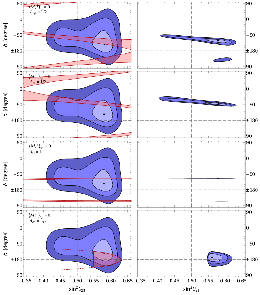
Figure 1: Left panels: the predictions of each model with normal ordering (NO) of the neutrino masses, and the phenomenologically allowed areas for NO, are displayed in pink and blue colours, respectively. In the fourth row, the conditions of model 4 are obeyed in the whole area surrounded by the red line (which might be further extended to lower values of $\sin^{2}{\theta_{23}}$), but $\sum m_{\nu}$ obeys the cosmological bound (53) only in the pink area. Right panels: in different shades of blue, the $1\sigma$, $2\sigma$, and $3\sigma$ regions defined by the simultaneous compliance with the model conditions and the phenomenological data. In the fourth row, only the region satisfying the cosmological bound has been depicted. The stars mark the best-fit points. Dashed lines at $\delta=\pi$ and $s_{23}^{2}=1/2$ have been drawn just for orientation. More details are given in subsection 4.2.

Each row of that figure corresponds to the model that is defined by the conditions that are written in the top-left corner of the left panel of the row, viz. to models 1, 2, 3, and 4, respectively. All these models are for a normal ordering of the neutrino masses, thus $m_{\mathrm{minimum}}=m_{1}$. In figure 1, just as in figures 3 and 4, we do not display any panels corresponding to model 5, because the predictions of models 4 and 5 are almost identical to each other.

In the left panels of figure 1 one sees, in different shades of blue, the $1\sigma$, $2\sigma$, and $3\sigma$ CL regions in the $s_{23}^{2}$–$\delta$ plane that are allowed by the phenomenological data of ref. [6]. The stars mark the best-fit value of $\left(s_{23}^{2},\ \delta\right)$. The blue regions in the left panels are identical in all four rows of figure 1. The red regions in those panels are specific to each model; they consist of points that

(a) perfectly obey each model’s constraints,

(b) satisfy the cosmological bound (53),

(c) and have $\chi^{2}_{(1)}-\chi^{2}_{(1),\mathrm{minimum}}\leq 11.83$, where $\chi^{2}_{(1),\mathrm{minimum}}$ is the smallest value of $\chi^{2}_{(1)}$ in each region of red points; $\chi^{2}_{(1)}-\chi^{2}_{(1),\mathrm{minimum}}\leq 11.83$ corresponds to the $3\sigma$ CL for a Gaussian distribution with two degrees of freedom (in this case, $s_{23}^{2}$ and $\delta$).

Comparing the red regions in the top-two left panels of figure 1 one observes the effects of $\mu$–$\tau$ interchange; the red bands in the second panel are identical to the ones in the first panel after the transformation $s_{23}^{2}\to 1-s_{23}^{2},\ \delta\to 180^{\circ}+\delta$. In model 4 (the same is valid for model 5) there is a strong correlation between $s_{23}^{2}$ and $\sum m_{\nu}$, which is depicted in the left panel of figure 2.

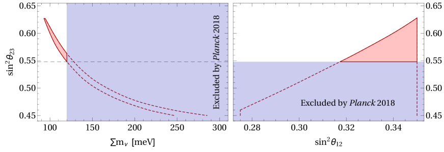
Figure 2: The correlation among $\sin^{2}{\theta_{23}}$, $\sin^{2}{\theta_{12}}$, and $\sum m_{\nu}$ in model 4. The pink-shaded areas in this figure are equivalent to the pink-shaded area in the bottom-left panel of figure 1. A dashed line marks the minimum value 0.548 of $\sin^{2}{\theta_{23}}$.

Because of that correlation and of the upper bound (53), $s_{23}^{2}$ cannot be lower than 0.548, as depicted through the pink-shaded area in the bottom-left panel of figure 1. If it were not for the bound (53), $s_{23}^{2}$ would be able to be much lower, as shown by the dashed red lines in that panel. Another interesting feature of model 4 is a large forbidden zone in the $s_{12}^{2}$–$s_{23}^{2}$ plane; that zone, with low $s_{12}^{2}$ and high $s_{23}^{2}$, can be observed in the right panel of figure 2.

In the right panels of figure 1 one sees, for each model 1–4, the points that have $\chi^{2}-\chi^{2}_{\mathrm{minimum}}$ smaller than 2.3 ($1\sigma$ or 68.27$\%$ CL), 6.18 ($2\sigma$ or 95.45$\%$ CL), and 11.83 ($3\sigma$ or 99.73$\%$ CL). In drawing the right panels we have used the full function $\chi^{2}=\chi^{2}_{(1)}+\chi^{2}_{(2)}+\chi^{2}_{(3)}$ instead of just $\chi^{2}_{(1)}$ like in the left panels—this is the reason why the areas in the right panels of figure 1 are not equal to the intersection of the pink and blue areas in the left panels; the pink areas in the left panels were drawn by using only $\chi^{2}_{(1)}$ in equation (55), while the areas in the right panels were drawn by using $\chi^{2}_{(1)}+\Delta\chi^{2}\left(s_{23}^{2},\delta\right)$. It should be stressed that, even though all four right panels of figure 1 have a light-blue-coloured zone corresponding to $\chi^{2}-\chi^{2}_{\mathrm{minimum}}<2.3$, that does not mean that all four models 1–4 fit the data equally well, because $\chi^{2}_{\mathrm{minimum}}$ is different for the four models. The values of $\chi^{2}_{\mathrm{minimum}}$ are given in the last row of table 1; they make clear that models 1 and 3 agree with the data almost perfectly, while model 2 is not quite as good and model 4 (and also model 5) is even worse. For instance, all the points with $\chi^{2}-\chi^{2}_{\mathrm{minimum}}<2.3$ for model 1 have $\chi^{2}<2.7$ and are therefore better than even the best point of model 4.

One sees in figure 1 that both models 1 and 3 display two different ‘solutions’, one of them with $\delta\sim-120^{\circ}$ and the other one with $\delta\approx 120^{\circ}$. Under complex conjugation of the lepton mixing matrix, i.e. under $\delta\to-\delta$, $\alpha_{21}\to-\alpha_{21}$, and $\alpha_{31}\to-\alpha_{31}$ the conditions defining each model remain invariant, but the phenomenological bounds on $\delta$ do not; this is the reason why, for instance for model 1, there are two solutions with symmetric values of the phases—but one of those solutions has much higher values of $\chi^{2}-\chi^{2}_{\mathrm{minimum}}$. For model 3 all the points of the second solution have $\chi^{2}-\chi^{2}_{\mathrm{minimum}}>9$ and therefore that solution does not appear in table 1.

Comparing the left and right panels of figure 1, one sees that all models 1–3 severely constrain the phase $\delta$, but they do not constrain $s_{23}^{2}$ by themselves alone. Model 4 has $s_{23}^{2}$ correlated with $\sum m_{\nu}$ and, even when $\sum m_{\nu}$ becomes very large (i.e. when the light neutrinos are almost degenerate), $s_{23}^{2}\gtrsim 0.418$ is constrained; after the addition of the cosmological bound (53) the constraint becomes much stronger. Model 4 also restricts $s_{12}^{2}$, see the right panel of figure 2.

Next look at figure 3.

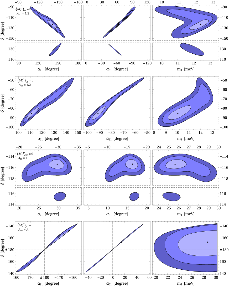
Figure 3: The same regions as in the right panels of figure 1 are now depicted in the $\delta$–$\alpha_{21}$ plane (left panels), $\delta$–$\alpha_{31}$ plane (central panels), and $\delta$–$m_{1}$ plane (right panels) for models 1, 2, 3, and 4, respectively, from top to bottom. For model 4, only the points obeying the cosmological bound are displayed.

There, one sees the same regions as in the right panels of figure 1, but now displaying the Majorana phases $\alpha_{21}$ and $\alpha_{31}$, and also the smallest neutrino mass $m_{1}$, against $\delta$. Only points that comply with the cosmological bound on $\sum m_{\nu}$ are displayed; this is not an effective constraint for models 1–3, but it severely constrains model 4 (and model 5).

In figure 4

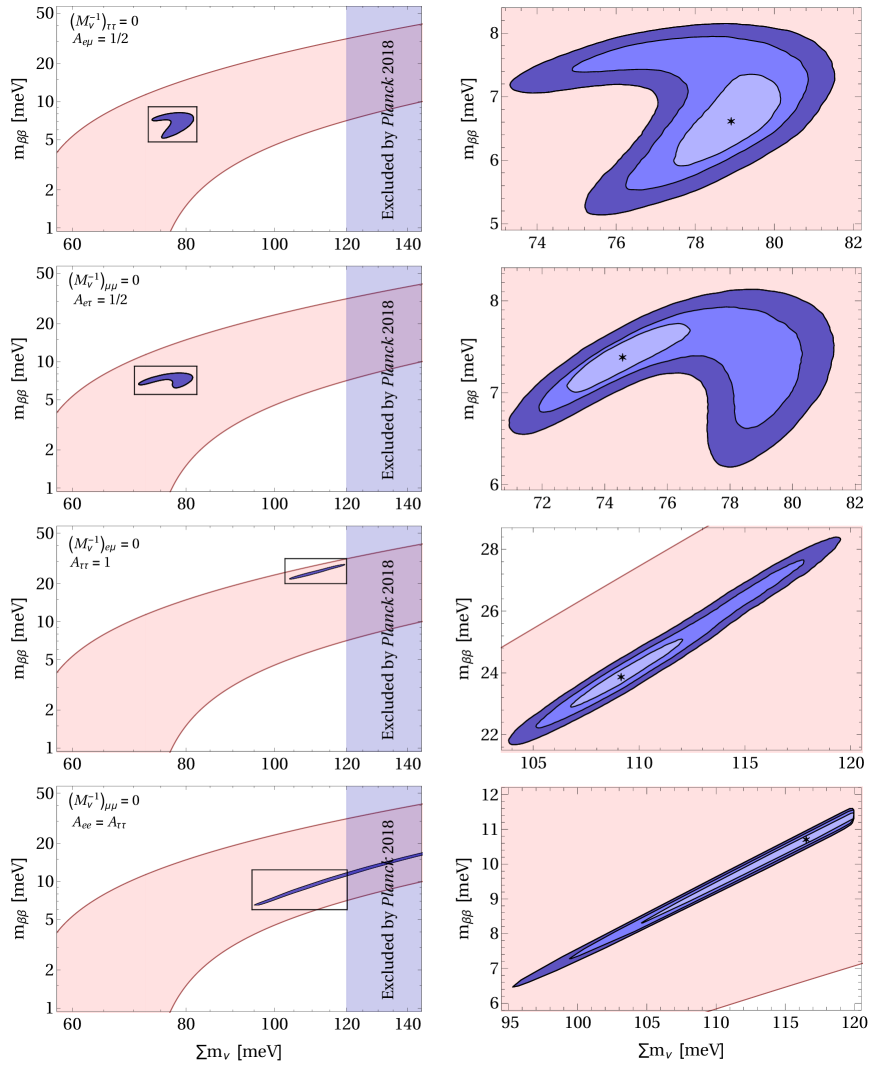
Figure 4: In the four rows one sees the predictions of models 1, 2, 3, and 4, respectively, for the sum of the light-neutrino masses and for the mass parameter responsible for neutrinoless $2\beta$ decay. Pink areas are allowed by phenomenology alone; blue areas include the conditions of each model. The right panels are zooms of the marked areas in the left panels.

one observes the predictions of each model 1–4 for the mass parameters $\sum m_{\nu}$ and $m_{\beta\beta}$. The pink areas in figure 4 are the same for all models and they are allowed by the phenomenological constraints only; the areas in various shades of blue are allowed at the $1\sigma$, $2\sigma$, and $3\sigma$ CL by the phenomenological constraints together with each model’s conditions. One sees that each model strongly constrains the mass parameters, restricting them to a much smaller range than the one allowed by phenomenology only. It was already clear from the right panels of figure 3 that models 1 and 2 work for much lower values of the neutrino masses than models 3 and 4; $m_{1}\sim 10$ meV for models 1 and 2 while $m_{1}\sim 25$ meV for models 3 and 4. This same fact is observed in figure 4, where $\sum m_{\nu}$—but not $m_{\beta\beta}$, which includes some interference effects—is much higher in models 3 and 4 than in models 1 and 2. Notice that a large otherwise-allowed range of model 4 has been eliminated by the cosmological bound on $\sum m_{\nu}$; the same may soon happen to model 3, which predicts $\sum m_{\nu}\gtrsim 105\,$meV.

We have summarized in table 1 the predictions of each of the models with NO.

model	1 (1st sol.)	1 (2nd sol.)	2	3	4
$m_{1}\left(\mbox{meV}\right)$	9.9 – 13.1	11.7 – 12.1	8.6 – 13.0	23.9 – 29.5	20.6 – 30.4
$\sum m_{\nu}\left(\mbox{meV}\right)$	74.0 – 81.2	77.7 – 78.7	71.4 – 80.9	104.7 – 118.6	97.2 – 120.0
$m_{\beta\beta}\left(\mbox{meV}\right)$	5.4 – 8.0	6.0 – 6.4	6.5 – 8.0	22.0 – 28.0	6.8 – 11.6
$m_{\mathrm{tritium}}\left(\mbox{meV}\right)$	13.3 – 15.9	14.7 – 15.0	12.3 – 15.8	25.5 – 30.8	22.5 – 31.6
$10\times s_{23}^{2}$	4.17 – 6.25	5.88 – 6.03	4.17 – 6.26	4.17 – 6.25	5.49 – 6.14
$\delta\left({}^{\circ}\right)$	216 – 268	125 – 132	263 – 309	242 – 246	149 – 224
$\alpha_{21}\left({}^{\circ}\right)$	204 – 250	143 – 148	103 – 144	327 – 339	163 – 203
$\alpha_{31}\left({}^{\circ}\right)$	39 – 94	300 – 308	260 – 303	341 – 350	$-37$ – 51
$\chi^{2}_{\mathrm{minimum}}$	0.39	8.99	1.68	0.67	3.58

Table 1: The $3\sigma$ bounds for various observables in the models with normal neutrino mass ordering. These bounds correspond to $\chi^{2}-\chi^{2}_{\mathrm{minimum}}\leq 9$, which is equivalent to $3\sigma$ CL for one degree of freedom; they take into account the cosmological bound $\sum m_{\nu}<0.12$ eV [14]. For model 5 the values are the same as for model 4, with the exceptions $10\times s_{23}^{2}$ (5.48 to 6.14), $\delta$ (154^∘ to 213^∘), $\alpha_{31}$ ($-36^{\circ}$ to $46^{\circ}$), and $\chi^{2}_{\mathrm{minimum}}$ (3.82).

In that table we only display points with $\chi^{2}-\chi^{2}_{\mathrm{minimum}}\leq 9$, therefore the ranges are somewhat narrower than the ones observed in the figures, where the $3\sigma$ regions have $\chi^{2}-\chi^{2}_{\mathrm{minimum}}\leq 11.83$. For the same reason, the second solution for model 3 does not appear in table 1.

The observables $s_{12}^{2}$, $s_{13}^{2}$, $\Delta m^{2}_{\mathrm{solar}}$, and $\Delta m^{2}_{\mathrm{atmospheric}}$ are not constrained by models 1–5, with the exception $s_{12}^{2}\in[0.320,\ 0.350]$ in models 4 and 5; this is not, however, because of the models themselves, but rather because of the cosmological bound, that leads those models to necessitate both a rather high $s_{23}^{2}$ and a rather high $s_{12}^{2}$.

4.3 Junction of models 4 and 5

Models 4 and 5 have almost the same predictions and, as a matter of fact, we may join them in only one model, defined by

$$\left(\mathcal{M}_{\nu}^{-1}\right)_{\mu\mu}=0\quad\mbox{and}\quad A_{ee}=A_{\tau\tau}=A_{\tau\tau}^{\ast}.$$ (56)

This model agrees with experiment and has $\chi^{2}_{\mathrm{minimum}}=4.22$, which is not much worse than either model 4 or model 5 separately. The CP-violating phases are eliminated: $\delta=\alpha_{21}=\pi$ and $\alpha_{31}=0$, rendering this model CP-conserving in the leptonic sector. The predictions for the mass observables and for $s_{23}^{2}$ are exactly the same as the ones displayed in table 1 for model 4.

The plus of this model is that it provides a clear-cut correlation among $s_{12}^{2}$, $s_{23}^{2}$, and $\sum m_{\nu}$. That correlation is displayed in figure 5.

Figure 5: The correlation among $s_{12}^{2}$, $s_{23}^{2}$, and the cosmological mass in a model uniting models 4 and 5 together. In the top row, the dashed line represents the cosmological bound (53). In the bottom row, the depicted areas all respect that bound.

On the other hand, this model requires both $s_{12}^{2}$ and $s_{23}^{2}$ to be quite above their best-fit values; that is the reason why $\chi^{2}_{\mathrm{minimum}}$ is rather high for this model.

4.4 Models 6 and 7

Figure 6 is analogous to figure 1. It features model 6 in its top row and model 7 in its bottom row.

Figure 6: Left panels: the predictions of each model with inverted ordering (IO) of the neutrino masses, and the phenomenologically allowed areas for IO, are displayed in pink and blue colours, respectively. The panels in the top row respect model 6 and the ones in the bottom row are for model 7. Right panels: in different shades of blue, the $1\sigma$, $2\sigma$, and $3\sigma$ regions defined by the simultaneous compliance with the each model’s conditions and the phenomenological data. The stars mark the best-fit points. Dashed horizontal lines at various values of $\delta$, and a vertical dashed line at $s_{23}^{2}=1/2$, have been drawn for orientation. More details are given in the text.

In the pink bands of the left panels one clearly sees the effect of the $\mu$–$\tau$ interchange symmetry in the models’ defining conditions: those bands are symmetric under $s_{23}^{2}\to 1-s_{23}^{2},\ \delta\to 180^{\circ}+\delta$. In the right panels one sees that both model 6 and model 7 have two different solutions. Those two solutions are more clearly visible in figure 7, wherein the first row displays both solutions of model 6 simultaneously and each of the two lower rows is devoted to one of the solutions of model 7. One of the two solutions of model 6 has much higher $\chi^{2}_{\mathrm{minimum}}$ than the other one. The two solutions of model 7 are quite distinct, with the preferred one having $\alpha_{21}\approx 0$ and $m_{\mathrm{minimum}}\approx 1.15$ meV, while the other one has $\alpha_{21}\sim 180^{\circ}$ and $m_{\mathrm{minimum}}$ twice as large.

Figure 7: The same regions as in the right panels of figure 6 are now depicted in the $\delta$–$\alpha_{21}$ plane (left panels), $\delta$–$\alpha_{31}$ plane (central panels), and $\delta$–$m_{3}$ plane (right panels). The top row is for model 6; the central and bottom rows are for each of the two solutions of model 7.

Also note, in the top central panel, that in model 6 there is an almost perfect linear relation between $\alpha_{31}$ and $\delta$; that relation may be expressed by the (approximate) equation $\alpha_{31}=178.007^{\circ}+1.98254\,\delta$.

In figure 8 one sees the predictions of the two IO models for the mass parameters. One observes once again the great difference between the two solutions of model 7, with one of them producing a much lower $m_{\beta\beta}$ than the other one. It is interesting to observe that both models admit $m_{\beta\beta}\sim 49$ meV, which is much higher than in the models with NO.

Figure 8: The predictions of models 6 (top row) and 7 (the other two rows) for the sum of the light-neutrino masses and for the mass parameter responsible for neutrinoless $2\beta$ decay. The pink areas are the ones allowed by phenomenology alone, for an inverted ordering of the neutrino masses; the blue areas include the constraints of each model. The right panels are zooms of the marked areas in the left panels.

model	6 (1st solution)	6 (2nd solution)	7 (1st solution)	7 (2nd solution)
$m_{3}\left(\mbox{meV}\right)$	1.05 – 1.25	1.11 – 1.18	1.05 – 1.25	1.99 – 3.39
$\sum m_{\nu}\left(\mbox{meV}\right)$	98.7 – 102.7	99.9 – 101.4	98.6 – 102.6	101.2 – 103.8
$m_{\beta\beta}\left(\mbox{meV}\right)$	47.5 – 49.4	48.1 – 48.8	47.5 – 49.4	16.0 – 27.5
$m_{\mathrm{tritium}}\left(\mbox{meV}\right)$	48.1 – 50.0	48.7 – 49.4	48.1 – 50.0	48.6 – 49.7
$10\times s_{23}^{2}$	5.27 – 6.27	4.29 – 4.61	4.23 – 6.27	4.87 – 5.18
$\delta\left({}^{\circ}\right)$	279 – 326	233 – 251	259.0 – 270.6	234 – 323
$\alpha_{21}\left({}^{\circ}\right)$	355.2 – 359.4	1.2 – 2.5	$-4.9$ – 2.9	148 – 233
$\alpha_{31}\left({}^{\circ}\right)$	17 – 113	287 – 323	$-3.4$ – 1.9	$-52$ – 80
$\chi^{2}_{\mathrm{minimum}}$	4.76	12.38	5.11	11.02

Table 2: The $3\sigma$ bounds for various observables in the models with inverted neutrino mass ordering. These bounds correspond to $\chi^{2}-\chi^{2}_{\mathrm{minimum}}\leq 9$. We have included the value $\chi^{2}_{(3)}=4.71254$, obtained by the NuFIT collaboration, in the computation of $\chi^{2}_{\mathrm{minimum}}$, therefore all the $\chi^{2}_{\mathrm{minimum}}$ are higher than the corresponding values for models with NO in table 1.

5 Summary and conclusions

In this paper we have shown that four new types of constraints on the lepton mass matrices, given in equations (49), can be derived through adequate symmetries imposed on renormalizable models furnished with three right-handed neutrinos and a type-I seesaw mechanism. Each of those constraints leads to predictive power for the CP-violating phase $\delta$ and for various neutrino-mass quantities. That predictive power has been studied in some detail in section 4 of the paper, especially taking into account the correlations between $\delta$ and the mixing anle $\theta_{23}$ displayed by the phenomenological data of ref. [6]. We have found that a total of seven models are able to fit the data at the $1\sigma$ level for at least one of the three phenomenological papers [4, 5, 6]. The predictions of each of our models have been given in tables 1 and 2.

Acknowledgements:

D.J. thanks Jordi Salvado for a detailed discussion about ref. [15]. D.J. thanks the Lithuanian Academy of Sciences for support through projects DaFi2018 and DaFi2019. The work of L.L. is supported by the Portuguese Fundação para a Ciência e a Tecnologia through the projects CERN/FIS-PAR/29436/2017, CERN/FIS-PAR/0004/2017, and UID/FIS/777/2019; those projects are partly funded by POCTI (FEDER), COMPETE, QREN, and the European Union.

References

• [1] P. Minkowski, $\mu\to e\gamma$ at a rate of one out of $10^{9}$​ muon decays?, Phys. Lett. 67B (1977) 421;
T. Yanagida, Horizontal gauge symmetry and masses of neutrinos, in Proceedings of the workshop on unified theory and baryon number in the universe (Tsukuba, Japan, 1979), O. Sawata and A. Sugamoto eds., KEK report 79-18, Tsukuba, 1979;
S. L. Glashow, The future of elementary particle physics, in Quarks and leptons, proceedings of the advanced study institute (Cargèse, Corsica, 1979), M. Lévy et al. eds., Plenum, New York, 1980;
M. Gell-Mann, P. Ramond, and R. Slansky, Complex spinors and unified theories, in Supergravity, D. Z. Freedman and F. van Nieuwenhuizen eds., North Holland, Amsterdam, 1979;
R. N. Mohapatra and G. Senjanović, Neutrino mass and spontaneous parity violation, Phys. Rev. Lett. 44 (1980) 912.
• [2] W. Grimus and L. Lavoura, The seesaw mechanism at arbitrary order: disentangling the small scale from the large scale, JHEP 0011 (2000) 042 [hep-ph/0008179].
• [3] M. Tanabashi et al. (Particle Data Group), Review of particle physics, Phys. Rev. D 98 (2018) 030001.
• [4] P. F. de Salas, D. V. Forero, C. A. Ternes, M. Tórtola, and J. W. F. Valle, Status of neutrino oscillations 2018: 3$\sigma$ hint for normal mass ordering and improved CP sensitivity, Phys. Lett. B 782 (2018) 633 [arXiv:1708.01186 [hep-ph]].
• [5] F. Capozzi, E. Lisi, A. Marrone, and A. Palazzo, Current unknowns in the three-neutrino framework, Prog. Part. Nucl. Phys. 102 (2018) 48 [arXiv:1804.09678 [hep-ph]].
• [6] I. Esteban, M. C. Gonzalez-Garcia, A. Hernandez-Cabezudo, M. Maltoni, and T. Schwetz, Global analysis of three-flavour neutrino oscillations: synergies and tensions in the determination of $\theta_{23}$, $\delta_{\mathrm{CP}}$, and the mass ordering, JHEP 1901 (2019) 106 [arXiv:1811.05487 [hep-ph]]. See also http://www.nu-fit.org, especially http://www.nu-fit.org/ ?q=node/177.
• [7] P. H. Frampton, S. L. Glashow, and D. Marfatia, Zeroes of the neutrino mass matrix, Phys. Lett. B 536 (2002) 79 [hep-ph/0201008].
• [8] L. Lavoura, Zeros of the inverted neutrino mass matrix, Phys. Lett. B 609 (2005) 317 [hep-ph/0411232].
• [9] P. M. Ferreira, L. Lavoura, and P. O. Ludl, Five models for lepton mixing, JHEP 1308 (2013) 113 [arXiv:1304.1654 [hep-ph]].
• [10] P. M. Ferreira, L. Lavoura, and P. O. Ludl, A new $A_{4}$ model for lepton mixing, Phys. Lett. B 726 (2013) 767 [arXiv:1306.1500 [hep-ph]].
• [11] W. Grimus, S. Kaneko, L. Lavoura, H. Sawanaka, and M. Tanimoto, $\mu$ $\tau$ antisymmetry and neutrino mass matrices, JHEP 0601 (2006) 110 [hep-ph/0510326].
• [12] W. Grimus and L. Lavoura, Maximal atmospheric neutrino mixing and the small ratio of muon to tau mass, J. Phys. G 30 (2004) 73 [hep-ph/0309050].
• [13] F. Feruglio, C. Hagedorn, and R. Ziegler, Lepton mixing parameters from discrete and CP symmetries, JHEP 1307 (2013) 027 [arXiv:1211.5560 [hep-ph]].
• [14] S. Vagnozzi, E. Giusarma, O. Mena, K. Freese, M. Gerbino, S. Ho, and M. Lattanzi, Unveiling $\nu$ secrets with cosmological data: Neutrino masses and mass hierarchy, Phys. Rev. D 96 (2017) 123503 [arXiv:1701.08172 [astro-ph.CO]];
Y. Akrami et al. [Planck Collaboration], Planck 2018 results. I. Overview and the cosmological legacy of Planck, arXiv:1807.06205 [astro-ph.CO].
• [15] J. Alcaide, J. Salvado, and A. Santamaria, Fitting flavour symmetries: the case of two-zero neutrino mass textures, JHEP 1807 (2018) 164 [arXiv:1806.06785 [hep-ph]].