Finite Element Error Estimates on Geometrically Perturbed Domains

Abstract

We develop error estimates for the finite element approximation of elliptic partial differential equations on perturbed domains, i.e. when the computational domain does not match the real geometry. The result shows that the error related to the domain can be a dominating factor in the finite element discretization error. The main result consists of $H^{1}$- and $L^{2}$-error estimates for the Laplace problem. Theoretical considerations are validated by a computational example.

1 Introduction

The main aim of this work is to develop finite element (FE) error estimates in the case when there is uncertainty with respect to the computational domain. We consider the question of how a domain related error affects the finite element discretization error. We use the conforming finite element method (FEM) which is well established in the scientific computing community and allows for a rigorous analysis of the approximation error ErnGuermond2004 .

Our motivation is as follows. The steps to obtain a mesh for FE computations often come with some uncertainty, for example related to empirical measurements or image processing techniques, e.g. medical image segmentation Oberkampf2006 ; OberkampfBook . Therefore, we often perform computations on a domain which is an approximation of the real geometry, i.e., the computational domain is close to but does not match the real domain. In this work we do not specify the source of the error, but we take the error into account by explicitly using the error laden reconstructed domains.

This theoretical result is of great importance for scientific computations. Vast numbers of engineering branches rely on the results of computational fluid dynamics simulations, where there is often uncertainty connected to the computational domain. A prime example of this is computational based medical diagnostics, where shapes are reconstructed from inverse problems, such as computer tomography. The assessment of error attributed to the limited spatial resolution of magnetic resonance techniques has been discussed in Moore1998 ; Moore1999 . For a survey on computational vascular fluid dynamics, where modeling and reconstruction related issues are discussed, we refer to Quarteroni2000 . Error analysis of computational models is a key factor for assessing the reliability for virtual predictions.

Uncertainties in the computational domain have been studied from the numerical perspective. Rigorous bounds for elliptic problems on random domains have been derived, for approximate problems defined on a sequence of domains that is supposed to converge in the set sense to a limit domain, for both Dirichlet Babuska2003 and Neumann Babuska2002 boundary conditions. Although our techniques are similar, we consider a case where the geometrical error is not small, but where it might dominate the discretization error.

When measurement data is available the accuracy of numerical predictions can be improved by data assimilation techniques. Applications of variational data assimilation in computational hemodynamics have been reviewed in DElia2012 . For recent developments we refer to Funke2019 and Nolte . On the other hand, the treatment of boundary uncertainty can be cast into a probabilistic framework. The domain mapping method is based entirely on stochastic mappings to transform the original deterministic/stochastic problem in a random domain into a stochastic problem in a deterministic domain, see Xiu2006 ; Tartakovsky2006 ; Harbrecht2016 . The perturbation method starts with a prescribed perturbation field at the boundary of a reference configuration and uses a shape Taylor expansion with respect to this perturbation field to represent the solution Harbrecht2008 . In Allaire2015 and Dambrine2015 a similar technique was used to incorporate random perturbations of a given domain in the context of shape optimization. Moreover, the fictitious domain approach and a polynomial chaos expansion have been applied in Canuto2007 . We note, that the probabilistic approach is beyond the scope of this work and the introduction of the boundary uncertainty as random variable increases the complexity of the problem.

The above approaches incorporate additional information on the domain reconstruction, such as measurement data or a probabilistic distribution of the approximation error. In comparison to these approaches our result can be seen as the worst case scenario. We only require that the distance between the two domains is bounded.

The analysis presented in this paper starts with well-known results regarding the finite element approximation on domains with curved boundaries. But in contrast to these estimates we cannot expect the error coming from the approximation of the geometry is small or even converging to zero. Instead we split the error into a geometric approximation error between real domain and perturbed domain and into an error coming from the finite element discretization of the problem on the perturbed domain. A central step is Lemma 4 which estimates the geometry perturbation. Having in mind that this error is not small and cannot be reduced by means of tuning the discretization, the typical application case is to balance both error contributions to efficiently reach the barrier of the geometry error. Theorem 3.2 gives such optimally balanced estimates that include both error contributions.

This paper is organized as follows. After this introduction, in Section 2 we introduce the mathematical setting and some required auxiliary results. Section 3 covers finite element discretization and proves the main results of this work. We illustrate our result with computational examples in Section 4.

2 Mathematical setting and auxiliary result

2.1 Notation

Let $\Omega\subset\mathds{R}^{d}$ be a domain with dimension $d\in\{2,3\}$. By $L^{2}(\Omega)$ we denote the Lebesgue space of square integrable functions equipped with the norm $\|\cdot\|_{\Omega}$. By $H^{1}(\Omega)$ we denote the space of $L^{2}(\Omega)$ functions with first weak derivative in $L^{2}(\Omega)$ and by $H^{m}(\Omega)$ for $m\in\mathds{N}_{0}$ we denote the corresponding generalizations with weak derivatives up to degree $m\in\mathds{N}_{0}$. The norms in $H^{m}(\Omega)$ are denoted by $\|\cdot\|_{H^{m}(\Omega)}$. For convenience we use the notation $H^{0}(\Omega)\coloneqq L^{2}(\Omega)$. By $H^{1}_{0}(\Omega)$ we denote the space of those $H^{1}(\Omega)$ functions that have vanishing trace on the domain’s boundary $\partial\Omega$ and we use the notation $H^{1}_{0}(\Omega;\Gamma)$ if the trace only vanishes on a part of the boundary, $\Gamma\subset\partial\Omega$. Further, by $(\cdot,\cdot)_{\Omega}$ we denote the $L^{2}(\Omega)$-scalar product and $\langle\cdot,\cdot\rangle_{\Gamma}$ the $L^{2}$-scalar product on a $d-1$ dimensional manifold $\Gamma$, e.g. $\Gamma=\partial\Omega$. Moreover, $[\partial_{n}\psi]$ is the jump of the normal derivative of $\psi$, i.e. for $x\in\Gamma$ with normal $\vec{n}$ (that is normal to $\Gamma$) $[\partial_{n}\psi](x):=\lim_{h\searrow 0}\partial_{n}\psi(x+h\vec{n})-\lim_{h\searrow 0}\partial_{n}\psi(x-h\vec{n}).$

2.2 Laplace equation and domain perturbation

On $\Omega\subset\mathds{R}^{d}$ let $f\in L^{2}(\Omega)$ be the given right hand side. We consider the Laplace problem with homogeneous Dirichlet boundary conditions,

$$-\Delta u=f\text{ in }\Omega,\quad u=0\text{ on }\partial\Omega.$$ (1)

The variational formulation of this problem is given by: find $u\in H^{1}_{0}(\Omega)$, such that

$$(\nabla u,\nabla\phi)_{\Omega}=(f,\phi)_{\Omega}\quad\forall\phi\in H^{1}_{0}(\Omega).$$ (2)

The boundary $\partial\Omega$ is supposed to have a parametrization in $C^{m+2}$, where $m\in\mathds{N}_{0}$. Given the additional regularity $f\in H^{m}(\Omega)$, $H^{0}(\Omega)\coloneqq L^{2}(\Omega)$, there exists a unique solution satisfying the a-priori estimate

$$\|u\|_{H^{m+2}(\Omega)}\leq c\|f\|_{H^{m}(\Omega)},$$ (3)

see e.g. evans .

In the following we assume that the real domain $\Omega$ is not exactly known but only given up to an uncertainty. We hence define a second domain, the reconstructed domain $\Omega_{r}$ with a boundary that allows for $C^{m+2}$ parametrization. The Hausdorff distance between both domains is then denoted by $\Upsilon\in\mathds{R}$,

$$\Upsilon:=\operatorname{dist}(\partial\Omega,\partial\Omega_{r}):=\max\{\adjustlimits{\sup}_{x\in\partial\Omega}{\inf}_{y\in\partial\Omega_{r}}|x-y|,\adjustlimits{\sup}_{y\in\partial\Omega_{r}}{\inf}_{x\in\partial\Omega}|x-y|\}.$$

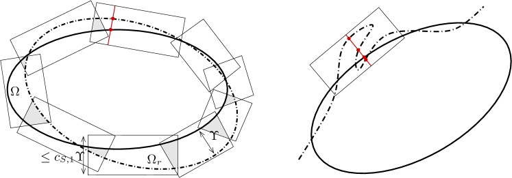
Figure 1: The domain $\Omega$ (bold line) and its reconstruction $\Omega_{r}$ (dashed). The cover of the domain remainders $S=(\Omega\setminus\Omega_{r})\cup(\Omega_{r}\setminus\Omega)$ by a set of rectangles. The left configuration fulfils Assumption 1. The height $h_{i}$ of each rectangle $R_{i}$ is bounded by $c_{S,1}\Upsilon$ and the intersections of each rectangle with the domain remainder $R_{i}\cap S$ do not overlap excessively. The shaded areas show the overlap. The right configuration is excluded by Assumption 1.

This distance $\Upsilon$ is not necessarily small. When it comes to spatial discretization we will be interested in both cases, $h\ll\Upsilon$ as well as $\Upsilon\ll h$, where $h>0$ is the mesh size. The two domains do not match and either domain can protrude from the other, see Figure 1. In order to prove our error estimates we require the following technical assumption on the relation between the two domains $\Omega$ and $\Omega_{r}$.

Assumption 1 (Domains)

Let $\Omega$ and $\Omega_{r}$ be two domains with $\Omega\cap\Omega_{r}\neq\emptyset$ and with Hausdorff distance $\Upsilon\in\mathds{R}$. Both boundaries allow for a local $C^{m+2}$ parametrization, $m\in\mathds{N}_{0}$. Let

$$S:=(\Omega_{r}\setminus\Omega)\cup(\Omega\setminus\Omega_{r}).$$

We assume that there exists a cover of $S$ by a finite number of open rectangles (or rectangular cuboids) $\{R_{1},\dots,R_{n(S)}\}$. Each rectangle $R_{i}$ is given as translation and rotation of $(0,h_{i})\times(0,t_{i})$ for $d=2$, or $(0,h_{i})\times(0,t_{i}^{1})\times(0,t_{i}^{2})$ for $d=3$, where the height $h_{i}$ is bounded by $h_{i}\leq c_{S,1}\,\Upsilon$ with a constant $c_{S,1}\geq 0$. Following conditions hold:

1. On each rectangle $R$, the boundary lines $\partial\Omega\cap R$ and $\partial\Omega_{r}\cap R$ allow for unique parametrizations $g^{R}_{\Omega}(t)$ and $g^{R}_{\Omega_{r}}(t)$ over the base $t$, or $(t^{1},t^{2})$ for $d=3$, respectively.

2. The area of the cover is bounded by the area of the remainder $S$, i.e.

   $$\big{|}\bigcup_{i=1}^{n(S)}R_{i}\cap S\big{|}\leq c_{S,2}|S|,$$

   where $c_{S,2}>0$ is a constant.

For the following we set $c_{S}:=\max\{c_{S,1},c_{S,2}\}$.

Figure 1 shows such a cover for different domain remainders. From Assumption A1 we deduce that each line through the height of the rectangle (marked in red in the figure) cuts each of the two boundaries exactly one time. The second assumption limits the overlap of the rectangles. These are shown as the shaded in the left sketch in Figure 1. Both assumptions on the domain are required for the proof of Lemma 3 that is based on Fubini’s integral theorem. A more flexible framework that allows for a wider variety of domains, e.g. with boundaries that feature hooks, could be based on the construction of a map between two boundary segments on $\partial\Omega_{r}$ and $\partial\Omega$. Such approaches play an important role in isogeometric analysis. We refer to Xu2011 and Xu2013 for examples on the construction of such maps.

To formulate the Laplace equation on the reconstructed domain $\Omega_{r}$ we must face the technical difficulty that the right hand side $f\in H^{m}(\Omega)$ is not necessarily defined on $\Omega_{r}$. We therefore weaken the assumptions on the right hand side.

Assumption 2 (Right hand side)

Let $f\in H^{m}_{\text{loc}}(\mathds{R}^{d})$, i.e. $f\in H^{m}(G)$ for each compact subset $G\subset\mathds{R}^{d}$. In addition we assume that the right hand side on $\Omega_{r}$ can be bounded by the right hand side on $\Omega$, i.e.

$$\|f\|_{H^{m}(\Omega_{r})}\leq c\|f\|_{H^{m}(\Omega)}.$$ (4)

An alternative would be to use Sobolev extension theorems to extend functions $f\in H^{m}(\Omega)$ from $\Omega$ to $\Omega_{r}$, see Calderon1961 .

On $\Omega_{r}$ we define the solution $u_{r}\in H^{1}_{0}(\Omega_{r})$ to the perturbed Laplace problem

$$(\nabla u_{r},\nabla\phi_{r})_{\Omega_{r}}=(f,\phi_{r})_{\Omega_{r}}\quad\forall\phi_{r}\in H^{1}_{0}(\Omega_{r}),$$ (5)

The unique solution to (5) satisfies the bound

$$\|u_{r}\|_{H^{m+2}(\Omega_{r})}\leq c\|f\|_{H^{m}(\Omega_{r})}\leq c\|f\|_{H^{m}(\Omega)}.$$ (6)

Remark 1 (Extension of the solutions)

A difficulty for deriving error estimates is that $u$ is defined on $\Omega$ and $u_{r}$ on $\Omega_{r}\neq\Omega$. Since the domains do not match, $u$ may not be defined on all of $\Omega_{r}$ and vice versa. To give the expression $u-u_{r}$ a meaning on all domains we extend both solutions by zero outside their defining domains, i.e. $u:=0$ on $\Omega_{r}\setminus\Omega$ and $u_{r}:=0$ on $\Omega\setminus\Omega_{r}$. Globally, both functions still have the regularity $u,u_{r}\in H^{1}(\Omega\cup\Omega_{r})$. We will use the same notation for discrete functions $u_{h}\in V_{h}$ defined on a mesh $\Omega_{h}$ and extend them by zero to $\mathds{R}^{d}$.  $\triangle$

The following preliminary results are necessary in the proof of the main estimates. They can be considered as variants of the trace inequality and of Poincaré’s estimate, respectively.

Lemma 3

Let $\gamma\in\mathds{R},\gamma>0$, $V\subset\mathds{R}^{d}$ and $W\subset\mathds{R}^{d}$ for $d\in\{2,3\}$ be two domains with boundaries $\partial V$ and $\partial W$ that satisfy Assumption 1 with distance

$$\gamma\coloneqq\operatorname{dist}(\partial V,\partial W).$$

For $\psi\in C^{1}(V)\cap C(\bar{V})$ it holds

$$\begin{split}&\|\psi\|_{\partial W\cap V}\leq c\Big{(}\|\psi\|_{\partial V}+\gamma^{\frac{1}{2}}\|\nabla\psi\|_{V\setminus W}\Big{)},\\ &\|\psi\|_{V\setminus W}\leq c\gamma^{\frac{1}{2}}\Big{(}\|\psi\|_{\partial V}+\gamma^{\frac{1}{2}}\|\nabla\psi\|_{V\setminus W}\Big{)},\end{split}$$ (7)

where the constants $c>0$ depend on $c_{S}$ from Assumption 1 and the curvature of the domain boundaries.

Proof

Let $R$ be one rectangle of the cover and let $x_{\partial W}=g^{R}_{W}(t)\in\partial(W\cap V)\cap R$, see Figure 2. By $x_{\partial V}=g^{R}_{V}(t)\in\partial(W\cap V)\cap R$ we denote the corresponding unique point on $\partial W\cap R$. The connecting line segment $\overline{x_{\partial V}x_{\partial W}}$ completely runs through $V\setminus W$, as, if the line would leave this remainder, it would cut each line more than once which opposes Assumption 1.b). Integrating the function $\psi$ along this line gives

$$\big{|}\psi(x_{\partial W})\big{|}^{2}\leq 2\big{|}\psi(x_{\partial V})\big{|}^{2}+2\big{|}\int_{x_{\partial V}}^{x_{\partial W}}\psi^{\prime}(s)\,\text{d}s\big{|}^{2}.$$

Applying Hölder’s inequality to the second term on the right hand side, with the length of the line bounded by $c_{S}\gamma$, we obtain

$$|\psi(x_{\partial W})|^{2}\leq 2|\psi(x_{\partial V})|^{2}+2c_{S}\gamma\int_{x_{\partial V}}^{x_{\partial W}}|\nabla\psi(s)|^{2}\,\text{d}s.$$

Using the parametrizations $x_{\partial W}=g^{R}_{W}(t)$ and $x_{\partial V}=g^{R}_{V}(t)$ we integrate over $t$ which gives

$$\int|\psi(g^{R}_{W}(t))|^{2}\,\text{d}t\leq\int|\psi(g^{R}_{V}(t))|^{2}\,\text{d}t+2c_{S}\gamma\int\int_{g^{R}_{V}(t)}^{g^{R}_{W}(t)}|\nabla\psi(s)|^{2}\,\text{d}s\,\text{d}t.$$ (8)

The volume integral on the right hand side is exactly the integral over $R\cap(V\setminus W)$. The boundary integrals can be interpreted as path integrals and therefore be estimated by

$$\frac{1}{\max_{t}\{1+|\nabla g^{R}_{W}(t)|^{2}\}}\int_{(\partial W\cap V)\cap R}|\psi|^{2}\,\text{d}s\\ \leq\frac{1}{\min_{t}\{1+|\nabla g^{R}_{V}(t)|^{2}\}}\int_{R\cap\partial V}|\psi|^{2}\,\text{d}s+2c_{S}\gamma\!\!\!\!\int_{R\cap(V\setminus W)}\!\!\!\!|\nabla\psi|^{2}\,\text{d}x.$$ (9)

As the boundaries allow for a $C^{2}$ parametrization, we estimate

$$\|\psi\|^{2}_{(\partial W\cap V)\cap R}\leq c(\partial V,\partial W)c_{S}\Big{(}\|\psi\|^{2}_{R\cap\partial V}+\gamma\|\nabla\psi\|^{2}_{R\cap S}\Big{)}.$$ (10)

Summation over all rectangles and estimation of all overlaps by means of Assumption 1 gives

$$\|\psi\|^{2}_{\partial W\cap V}\leq c(\partial V,\partial W)c_{S}\Big{(}\|\psi\|^{2}_{\partial V}+\gamma\|\nabla\psi\|^{2}_{V\setminus W}\Big{)}.$$

For $\psi\in H^{1}_{0}(V)$, the term on $\partial V$ vanishes.

[capbesideposition=left,top,capbesidewidth=0.66]figure[]

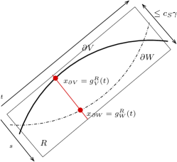
Figure 2: Illustration of the proof of Lemma 3. Points in each rectangle $R$ can be represented by local coordinates $(t,s)$, where $0\leq s\leq c_{S}\gamma$ and the range of $t$ depends on the size of the rectangle. The two boundary segments are given by the (smooth) parametrizations $g^{R}_{V}(t)$ and $g^{R}_{W}(t)$. Each line in the direction of $s$ cuts both boundaries exactly once. In the 3d setting, the base is represented by two coordinates $\mathbf{t}=(t_{1},t_{2})$.

To show the second estimate on $V\setminus W$ we again pick one rectangle $R$ and consider a point $x\in V\setminus W$ on the line connecting $x_{\partial V}=g^{R}_{V}(t)$ and $x_{\partial W}=g^{R}_{W}(t)$ such that we introduce the notation $x=x(t,s)$. By the same arguments as above it holds

$$|\psi(x(t,s))|^{2}\leq 2|\psi(g^{R}_{V}(t))|^{2}+2c_{S}\gamma\int\int_{x(t)}^{g^{R}_{V}(t)}|\nabla\psi|^{2}\,\text{d}s\text{d}t.$$

We integrate over $s$ and $t$ to obtain

$$\|\psi(x)\|^{2}_{R\cap(V\setminus W)}\leq\frac{2}{\min_{t}\{1+|\nabla g^{R}_{V}(t)|^{2}\}}\gamma\|\psi\|^{2}_{R\cap\partial V}+2c_{S}\gamma^{2}\|\nabla\psi\|^{2}_{R\cap(V\setminus W)}.$$

Summing over all rectangles gives the desired result.

The above lemma is later used in such a way that $V$ and $W$ can be substituted as both $\Omega$ and $\Omega_{r}$, specifically to the case of use.

We continue by estimating the difference between the solutions of the Laplace equations on $\Omega$ and on $\Omega_{r}$.

Lemma 4

Let $\Omega,\Omega_{r}\in\mathds{R}^{d}$ with $\partial\Omega,\partial\Omega_{r}\in C^{m+2}$ satisfying $\operatorname{dist}(\partial\Omega,\partial\Omega_{r})<\Upsilon$ as well as Assumption 1. Furthermore, let $f\in L^{2}_{\text{loc}}(\mathds{R}^{d})$ satisfy Assumption 2 and let $f_{r}\coloneqq f|_{\Omega_{r}}$. For the solutions $u\in H^{1}_{0}(\Omega)\cap H^{2}(\Omega)$ and $u_{r}\in H^{1}_{0}(\Omega_{r})\cap H^{2}(\Omega_{r})$ to (2) and (5) respectively, it holds that

$$\|u-u_{r}\|_{\Omega}+\Upsilon^{\frac{1}{2}}\|\nabla(u-u_{r})\|_{\Omega}\leq c\Upsilon\|f\|_{\Omega\cup\Omega_{r}}.$$

Proof

(i) We continuously extend $u$ and $u_{r}$ by zero to $\mathds{R}^{d}$, c.f. Remark 1, such that $u-u_{r}\in H^{1}(\Omega\cup\Omega_{r})$ is well defined. We separate the domains of integration and integrate by parts

$$\begin{split}\|\nabla(u-u_{r})\|_{\Omega}^{2}=&\big{(}\nabla(u-u_{r}),\nabla(u-u_{r})\big{)}_{\Omega\cap\Omega_{r}}+\big{(}\nabla(u-u_{r}),\nabla(u-u_{r})\big{)}_{\Omega\setminus\Omega_{r}}\\ =&-\big{(}\Delta(u-u_{r}),u-u_{r}\big{)}_{\Omega}+\langle\partial_{n}(u-u_{r}),u-u_{r}\rangle_{\partial(\Omega\cap\Omega_{r})}\\ &\quad+\langle\partial_{n}(u-u_{r}),u-u_{r}\rangle_{\partial(\Omega\setminus\Omega_{r})}.\end{split}$$ (11)

Combining the boundary terms on the right-hand side of (11), into an integral over $\partial\Omega$ and a jump term over $\partial\Omega_{r}\cap\Omega$, we obtain

$$\begin{split}\|\nabla(u-u_{r})\|_{\Omega}^{2}=&-\big{(}\Delta(u-u_{r}),u-u_{r}\big{)}_{\Omega}+\langle\partial_{n}(u-u_{r}),u-u_{r}\rangle_{\partial\Omega}\\ &\quad+\langle[\partial_{n}(u-u_{r})],u-u_{r}\rangle_{\partial\Omega_{r}\cap\Omega}.\end{split}$$ (12)

In $\Omega\cap\Omega_{r}$ it holds $f=f_{r}$ and hence (weakly) $-\Delta(u-u_{r})=0$, such that

$$-(\Delta(u-u_{r}),u-u_{r})_{\Omega}=-(\Delta(u-u_{r}),u-u_{r})_{\Omega\cap\Omega_{r}}-(\Delta u,u)_{\Omega\setminus\Omega_{r}}\!\!=(f,u)_{\Omega\setminus\Omega_{r}}.$$ (13)

On $\partial\Omega$ it holds $u=0$ and on $\partial\Omega_{r}\cap\Omega$ it holds $u_{r}=0$. Further, since $u\in H^{2}(\Omega)$ it holds that $[\partial_{n}u]=0$ on $\partial\Omega_{r}\cap\Omega$. Finally, $u_{r}=0$ on $\Omega\setminus\Omega_{r}$, such that the boundary terms reduce to

$$\langle\partial_{n}(u-u_{r}),u-u_{r}\rangle_{\partial\Omega}+\langle[\partial_{n}(u-u_{r})],u-u_{r}\rangle_{\partial\Omega_{r}\cap\Omega}\\ =-\langle\partial_{n}(u-u_{r}),u_{r}\rangle_{\partial\Omega\cap\Omega_{r}}-\langle\partial_{n}u_{r},u\rangle_{\partial\Omega_{r}\cap\Omega}.$$ (14)

Combining (12)-(14) and using the Cauchy-Schwarz inequality, we estimate

$$\|\nabla(u-u_{r})\|_{\Omega}^{2}\leq\|f\|_{\Omega\setminus\Omega_{r}}\|u\|_{\Omega\setminus\Omega_{r}}\\ +\|\partial_{n}(u-u_{r})\|_{\partial\Omega\cap\Omega_{r}}\|u_{r}\|_{\partial\Omega\cap\Omega_{r}}+\|\partial_{n}u\|_{\partial\Omega_{r}\cap\Omega}\|u\|_{\partial\Omega_{r}\cap\Omega}.$$ (15)

Since $u,u_{r}\in H^{2}(\Omega\cap\Omega_{r})$, the trace inequality gives

$$\|\nabla(u-u_{r})\|_{\Omega}^{2}\leq\|f\|_{\Omega\setminus\Omega_{r}}\|u\|_{\Omega\setminus\Omega_{r}}\\ +c\big{(}\|u\|_{H^{2}(\Omega)}+\|u_{r}\|_{H^{2}(\Omega_{r})}\big{)}\big{(}\|u_{r}\|_{\partial\Omega\cap\Omega_{r}}+\|u\|_{\partial\Omega_{r}\cap\Omega}\big{)}.$$ (16)

Applying Lemma 3 twice: to $\psi=u$ and to $\psi=\nabla u$ (same for $u_{r})$, and extending the norms from $\Omega\setminus\Omega_{r}$ to $\Omega$ and from $\Omega_{r}\setminus\Omega$ to $\Omega_{r}$ give the bounds

$$\|u\|_{\partial\Omega_{r}\cap\Omega} \leq c\Upsilon^{\frac{1}{2}}\|\nabla u\|_{\Omega\setminus\Omega_{r}}\leq c\Upsilon\Big{(}\|\nabla u\|_{\partial\Omega}+\Upsilon^{\frac{1}{2}}\|u\|_{H^{2}(\Omega)}\Big{)},$$ (17)

$$\|u_{r}\|_{\partial\Omega\cap\Omega_{r}} \leq c\Upsilon^{\frac{1}{2}}\|\nabla u_{r}\|_{\Omega_{r}\setminus\Omega}\leq c\Upsilon\Big{(}\|\nabla u_{r}\|_{\partial\Omega_{r}}+\Upsilon^{\frac{1}{2}}\|u_{r}\|_{H^{2}(\Omega_{r})}\Big{)}.$$

With the trace inequality and the a priori estimates $\|u\|_{H^{2}(\Omega)}\leq c\|f\|_{\Omega}$ and $\|u_{r}\|_{H^{2}(\Omega_{r})}\leq c\|f_{r}\|_{\Omega_{r}}\leq c\|f\|_{\Omega}$ we obtain the bounds

$$\|u\|_{\partial\Omega_{r}\cap\Omega}\leq c\Upsilon\|f\|_{\Omega},\quad\|u_{r}\|_{\partial\Omega\cap\Omega_{r}}\leq c\Upsilon\|f\|_{\Omega}.$$ (18)

Using the fact that $u=0$ on $\partial\Omega$ we apply (7) twice and use the trace inequality to get the estimate

$$\|u\|_{\Omega\setminus\Omega_{r}}\leq c\Upsilon\|\nabla u\|_{\Omega\setminus\Omega_{r}}\leq c\Upsilon^{\frac{3}{2}}\Big{(}\|u\|_{H^{2}(\Omega)}+\Upsilon^{\frac{1}{2}}\|u\|_{H^{2}(\Omega)}\Big{)}\leq c\Upsilon^{\frac{3}{2}}\|f\|_{\Omega}.$$ (19)

We can then estimate $\|f\|_{\Omega\setminus\Omega_{r}}\leq\|f\|_{\Omega}$ by extending to the complete domain. Combining (16) with (18) and (19) we obtain the estimate

$$\|\nabla(u-u_{r})\|^{2}_{\Omega}\leq c\Big{(}\Upsilon^{\frac{3}{2}}+\Upsilon\Big{)}\|f\|^{2}_{\Omega},$$

which concludes the $H^{1}$-norm bound.

(ii) For the $L^{2}$-estimate we introduce the adjoint problem

$$z\in H^{1}_{0}(\Omega):\quad-\Delta z=\frac{u-u_{r}}{\|u-u_{r}\|_{\Omega}}\text{ in }\Omega,$$

which allows for a unique solution satisfying the a-priori bound $\|z\|_{H^{2}(\Omega)}\leq c_{s}$ with the stability constant $c_{s}<\infty$. Testing with $u-u_{r}$ and integrating by parts twice gives

$$\|u-u_{r}\|_{\Omega}= -(z,\Delta(u-u_{r}))_{\Omega}+\langle z,\partial_{n}(u-u_{r})\rangle_{\partial\Omega}$$

$$\quad+\langle z,[\partial_{n}(u-u_{r})]\rangle_{\partial\Omega_{r}\cap\Omega}-\langle\partial_{n}z,u-u_{r}\rangle_{\partial\Omega}.$$

It holds $z=0$ and $u=0$ on $\partial\Omega$, $[\partial_{n}u]=0$ on $\partial\Omega_{r}\cap\Omega$ and $-\Delta(u-u_{r})=0$ in $\Omega\cap\Omega_{r}$ such that we get

$$\|u-u_{r}\|_{\Omega} =(z,f)_{\Omega\setminus\Omega_{r}}-\langle z,\partial_{n}u_{r}\rangle_{\partial\Omega_{r}\cap\Omega}+\langle\partial_{n}z,u_{r}\rangle_{\partial\Omega}$$

$$\leq\|z\|_{\Omega\setminus\Omega_{r}}\|f\|_{\Omega\setminus\Omega_{r}}+\|z\|_{\partial\Omega_{r}\cap\Omega}\|\partial_{n}u_{r}\|_{\partial\Omega_{r}\cap\Omega}+\|\partial_{n}z\|_{\partial\Omega}\|u_{r}\|_{\partial\Omega}.$$

The boundary terms $\|z\|_{\partial\Omega_{r}\cap\Omega}$ and $\|u_{r}\|_{\partial\Omega}$ are estimated with Lemma 3, the normal derivatives by the trace inequality and the terms on $\Omega\setminus\Omega_{r}$ by (7)

$$\|u-u_{r}\|_{\Omega}\leq c\Upsilon^{\frac{3}{2}}\|z\|_{H^{2}(\Omega)}\|f\|_{\Omega}+c\Upsilon\|z\|_{H^{2}(\Omega)}\|u_{r}\|_{H^{2}(\Omega_{r})}+c\Upsilon\|z\|_{H^{2}(\Omega)}\|u_{r}\|_{H^{2}(\Omega_{r})}.$$

The $L^{2}$-norm estimate follows by using the bounds $\|u\|_{H^{2}(\Omega)}\leq c\|f\|_{\Omega}$, $\|u_{r}\|_{H^{2}(\Omega_{r})}\leq c\|f\|_{\Omega}$ and $\|z\|_{H^{2}(\Omega)}\leq c$.

Remark 2

The estimate $\|f\|_{\Omega\setminus\Omega_{r}}\leq c\|f\|_{\Omega}$ is not optimal. Further powers of $\Upsilon$ are easily generated at the cost of a higher right hand side regularity. Also, the estimate $\|\partial_{n}(u-u_{r})\|\leq c(\|u\|_{H^{2}(\Omega)}+\|u_{r}\|_{H^{2}(\Omega_{r})})$ by Cauchy Schwarz and the trace inequality could be enhanced to produce powers of $\Upsilon$. The limiting term in (12) however is the boundary integral $|\langle\partial_{n}u_{r},u\rangle_{\partial\Omega_{r}\cap\Omega}|=\mathcal{O}(\Upsilon^{\frac{1}{2}})$ which is optimal in the $H^{1}$-estimate. In Remark 4 and Corollary 1 we present an estimate that focuses on the intersection $\Omega\cap\Omega_{r}$ only and that allows us to improve the order to $\mathcal{O}(\Upsilon)$ in the $H^{1}$-case by avoiding exactly this boundary integral.  $\triangle$

3 Discretization

The starting point of a finite element discretization is the mesh of the domain $\Omega$. In our setting we do not mesh $\Omega$ directly, because the domain $\Omega$ is not exactly known. Instead, we consider a mesh of the reconstructed domain $\Omega_{r}$.

We partition $\Omega_{r}$ into a parametric triangulation $\Omega_{h}$, consisting of open elements $T\subset\mathds{R}^{d}$. Each element $T\in\Omega_{h}$ stems from a unique reference element $\hat{T}$ which is a simple geometric structure such as a triangle, quadrilateral or tetrahedron. The numerical examples in Section 4 are based on quadrilateral meshes. The map $T_{T}:\hat{T}\to T$ is a polynomial of degree $r\in\mathds{N}$. We will consider iso-parametric finite element spaces, that are based on polynomials of the same degree $r\geq 1$. In the following we assume structural and shape regularity of the mesh such that standard interpolation estimates

$$\|\nabla^{k}(u_{r}-I_{h}u_{r})\|_{T} \leq ch^{r+1-k}\|u_{r}\|_{H^{r+1}(T)},\quad k=0,\dots,r\leq m,$$ (20)

$$\|\nabla^{k}(u_{r}-I_{h}u_{r})\|_{\partial T} \leq ch^{r+\frac{1}{2}-k}\|u_{r}\|_{H^{r+1}(T)},\quad k=0,\dots,r\leq m,$$

will hold for all elements $T\in\Omega_{h}$, c.f. Bernardi1989 . The discretization parameter $h$ represents the size of the largest element in the mesh. See (Richter2017, , Section 4.2.2) for a detailed description.

On the reference element $\hat{T}$ let $\hat{P}$ be a polynomial space of degree $r$, e.g.

$$\hat{P}\;\widehat{=}\;Q^{r}:=\operatorname{span}\{x_{1}^{\alpha_{1}}\cdots x_{d}^{\alpha_{d}}\;:\;0\leq\alpha_{1},\dots,\alpha_{d}\leq r\}$$

on quadrilateral and hexahedral meshes. Then, the finite element space $V_{h}^{r}$ on the mesh $\Omega_{h}$ is defined as

$$V_{h}^{r}=\{\phi_{h}\in C(\bar{\Omega}_{h})\;:\;\phi_{h}\circ T_{T}\in\hat{P}\text{ on every }T\in\Omega_{h}\}.$$

This parametric finite element space does not exactly match the domain $\Omega_{r}$. Given an iso-parametric mapping of degree $r$ it holds $\operatorname{dist}(\partial\Omega_{r},\partial\Omega_{h})=\mathcal{O}(h^{r+1})$ and finite element approximation error and geometry approximation error are balanced. Iso-parametric finite elements for the approximation on domains with curved boundaries are well established ErgatoudisIronsZienkiewicz1968 , optimal interpolation and finite element error estimates have been presented in (Ciarlet2002, , Section 4.4). The case of higher order elements with optimal order energy norm estimates is covered in Lenoir1986 . From (Richter2017, , Theorem 4.37) we cite the following approximation result for the iso-parametric approximation of the Laplace equation that also covers the $L^{2}$-error and which is formulated in a similar notation.

Theorem 3.1

Let $m\in\mathds{N}_{0}$ and let $\Omega_{r}$ be a domain with a boundary that allows for a parametrization of degree $m+2$. Let $f_{r}\in H^{m}(\Omega_{r})$ and $u_{h}\in V_{h}^{r}\cap H^{1}_{0}(\Omega_{h})$ be the iso-parametric finite element discretization of degree $1\leq r\leq m+1$

$$(\nabla u_{h},\nabla\phi_{h})_{\Omega_{h}}=(f_{r},\phi_{h})_{\Omega_{h}}\quad\forall\phi_{h}\in V_{h}^{r}.$$

It holds

$$\|u_{r}-u_{h}\|_{H^{1}(\Omega_{r})}\leq ch^{r}\|f_{r}\|_{H^{r-1}(\Omega_{r})},\quad\|u_{r}-u_{h}\|_{\Omega_{r}}\leq ch^{r+1}\|f_{r}\|_{H^{r-1}(\Omega_{r})}.$$

We formulated the error estimate on the domain $\Omega_{r}$ although the finite element functions are given on $\Omega_{h}$ only. To give Theorem 3.1 meaning, we consider all functions extended by zero as described in Remark 1. Combining these preliminary results directly yields the a priori error estimates.

Theorem 3.2

Let $m\in\mathds{N}_{0}$, $\Omega$ and $\Omega_{r}$ be domains with $C^{m+2}$ boundary, distance $\Upsilon$ and that satisfy Assumption 1. Let $\Omega_{h}$ be the iso-parametric mesh of $\Omega_{r}$ with degree $1\leq r\leq m+1$ and let $f\in H^{r-1}_{loc}(\mathds{R}^{d})$ satisfy Assumption 2. For the finite element error between the fully discrete solution $u_{h}\in V_{h}^{r}$

$$(\nabla u_{h},\nabla\phi_{h})_{\Omega_{h}}=(f,\phi_{h})_{\Omega_{h}}\quad\forall\phi_{h}\in V_{h}^{r}$$

and the true solution $u\in H^{1}_{0}(\Omega)\cap H^{m+2}(\Omega)$ it holds

$$\|u-u_{h}\|_{H^{1}(\Omega)}\leq c\big{(}\Upsilon^{\frac{1}{2}}+h^{r}\big{)}\|f\|_{H^{r-1}(\Omega)},$$

as well as

$$\|u-u_{h}\|_{\Omega}\leq c(\Upsilon+h^{r+1})\|f\|_{H^{r-1}(\Omega)}.$$

Proof

(i) We start with the $H^{1}$ error. Inserting $\pm u_{r}$ and extending the finite element error $u_{r}-u_{h}$ from $\Omega$ to $\Omega_{r}$, where a small remainder appears, we have

$$\|\nabla(u-u_{h})\|_{\Omega}^{2}\leq 2\Big{(}\|\nabla(u-u_{r})\|_{\Omega}^{2}+\|\nabla(u_{r}-u_{h})\|_{\Omega_{r}}^{2}+\|\nabla(u_{r}-u_{h})\|^{2}_{\Omega\setminus\Omega_{r}}\Big{)}.$$ (21)

The first and the second term on the right hand side are estimated by Lemma 4 and Theorem 3.1 and, since $u_{r}=0$ on $\Omega\setminus\Omega_{r}$, we obtain

$$\|\nabla(u-u_{h})\|_{\Omega}^{2}\leq c\Big{(}\Upsilon+h^{2r}\Big{)}\|f\|_{H^{r-1}(\Omega)}^{2}+2\|\nabla u_{h}\|^{2}_{\Omega\setminus\Omega_{r}}.$$ (22)

We continue with the remainder $\nabla u_{h}$ on $\Omega\setminus\Omega_{r}$, which is non-zero on $\Omega_{h}$ only

$$\|\nabla u_{h}\|_{\Omega\setminus\Omega_{r}}^{2}=\|\nabla u_{h}\|^{2}_{(\Omega_{h}\setminus\Omega_{r})\cap(\Omega\setminus\Omega_{r})}.$$

This remaining stripe has the width

$$\gamma_{h,\Upsilon}\coloneqq{\cal O}(\min\{h^{r+1},\Upsilon\}),$$

and we apply Lemma 3 to get

$$\|\nabla u_{h}\|_{(\Omega\setminus\Omega_{r})\cap(\Omega_{h}\setminus\Omega_{r})}^{2}\leq c\gamma_{h,\Upsilon}\|\nabla u_{h}\|_{\partial\Omega_{r}}^{2}+c\gamma_{h,\Upsilon}^{2}\|\nabla^{2}u_{h}\|_{\Omega_{h}\setminus\Omega_{r}}^{2},$$ (23)

where the second derivative $\nabla^{2}u_{h}$ is understood element wise. This term is extended to $\Omega_{h}$ and with the inverse estimate and the a priori estimate for the discrete solution we obtain with $\gamma_{h,\Upsilon}^{2}={\cal O}(h^{2r+2})$ that

$$\gamma_{h,\Upsilon}^{2}\|\nabla^{2}u_{h}\|_{\Omega_{h}\setminus\Omega_{r}}^{2}\leq c_{inv}\gamma_{h,\Upsilon}^{2}\ h^{-2}\|\nabla u_{h}\|_{\Omega_{h}}^{2}\leq c_{inv}h^{2r}\|f\|_{\Omega_{h}}^{2}\leq ch^{2r}\|f\|^{2}_{\Omega}.$$ (24)

To the first term on the right hand side of (23) we add $\pm u_{r}$ and $\pm I_{h}u_{r}$, the nodal interpolation of $u_{r}$ into the finite element space

$$\gamma_{h,\Upsilon}\|\nabla u_{h}\|^{2}_{\partial\Omega_{r}}\leq c\gamma_{h,\Upsilon}\big{(}\|\nabla u_{r}\|^{2}_{\partial\Omega_{r}}+\|\nabla(u_{r}-I_{h}u_{r})\|^{2}_{\partial\Omega_{r}}+\|\nabla(u_{h}-I_{h}u_{r})\|^{2}_{\partial\Omega_{r}}\big{)}.$$ (25)

Here, the first and last terms are estimated with the trace inequalities and, in the case of the discrete term with the inverse inequality, followed by adding $\pm u_{r}$ we get

$$\gamma_{h,\Upsilon}\|\nabla u_{h}\|^{2}_{\partial\Omega_{r}}\leq c\Upsilon\|f\|_{L^{2}(\Omega)}^{2}+ch^{r+1}\|\nabla(u_{r}-I_{h}u_{r})\|^{2}_{\partial\Omega_{r}}\\ +ch^{r}\|\nabla(u_{r}-I_{h}u_{r})\|^{2}_{\Omega_{r}}+h^{r}\|\nabla(u_{h}-u_{r})\|^{2}_{\Omega_{r}}.$$ (26)

We used both $\gamma_{h,\Upsilon}={\cal O}(h^{r+1})$ and $\gamma_{h,\Upsilon}={\cal O}(\Upsilon)$. Then, collecting all terms in (22)-(26) and using the interpolation estimates as well as Theorem 3.1 we finally get

$$\|\nabla(u-u_{h})\|^{2}_{\Omega}\leq c\big{(}\Upsilon+h^{2r}\big{)}\|f\|_{H^{r-1}(\Omega)}^{2}+ch^{3r-1}\|f\|_{H^{r-1}(\Omega)}^{2},$$ (27)

which shows the a priori estimate since $3r-1\leq 2r$ for all $r\geq 1$.

(ii) For the $L^{2}$-error we proceed in the same way, but the remainder appearing in (21) does not carry any derivative, such that, instead of (23) the optimal order variant of Lemma 3 with integration to the boundary $\partial\Omega_{h}$, where $u_{h}=0$, can be applied, i.e.

$$\|u-u_{h}\|^{2}_{\Omega}\leq c\Big{(}\|u-u_{r}\|^{2}_{\Omega}+\|u_{r}-u_{h}\|_{\Omega_{r}}^{2}+\Upsilon^{2}\|\nabla u_{h}\|^{2}_{\Omega\setminus\Omega_{r}}\Big{)}.$$

The $L^{2}$-estimate directly follows with Lemma 4, Theorem 3.1 and by the a priori estimate $\|\nabla u_{h}\|^{2}_{\Omega\setminus\Omega_{r}}\leq c\|\nabla u_{h}\|^{2}_{\Omega_{h}}\leq c\|f\|^{2}_{\Omega_{r}}$.

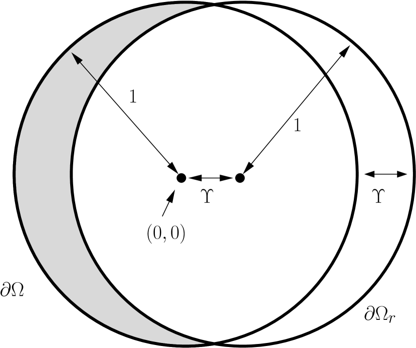
On $\Omega=B_{1}(0)$ and $\Omega_{r}=B_{1}(\Upsilon)$ consider $-\Delta u=4$ and $-\Delta u_{r}=4$, respectively with homogeneous Dirichlet conditions and the solutions

$$u(x,y)=1-x^{2}-y^{2},\;u_{r}(x,y)=1-(x-\Upsilon)^{2}-y^{2}$$

and the errors

$$\|\nabla(u-u_{r})\|_{\Omega}=\sqrt{8}\Upsilon^{\frac{1}{2}}+\mathcal{O}(\Upsilon),\;\|u-u_{r}\|_{\Omega}=\sqrt{\pi}\Upsilon+\mathcal{O}(\Upsilon^{3}).$$

Figure 3: Illustration concerning Remark 4. The error estimates for $u-u_{h}$ are optimal, if the error is evaluated on $\Omega$. The lowest order terms $\mathcal{O}(\Upsilon^{\frac{1}{2}})$ appear in the shaded area $\Omega\setminus\Omega_{r}$ where $u_{r}$ and (most of) $u_{h}$ are zero.

Remark 3 (Polygonal domains)

In two dimensions, the extension of the error estimates to the case of convex polygonal domains, where $u\in H^{2}(\Omega)$ and $u_{r}\in H^{2}(\Omega_{r})$, is relatively straightforward. In this case, $\Omega_{h}$ fits $\Omega_{r}$ such that the finite element error $u_{r}-u_{h}$ can be estimated with the standard a priori result $\|u_{r}-u_{h}\|+h\|\nabla(u_{r}-u_{h})\|\leq c\|f\|$. The extension of Lemma 3, which locally requires smoothness of the parametrizations $g^{R}_{W}(\cdot)$ and $g^{R}_{V}(\cdot)$, see steps (8)-(10), can be accomplished by refining the cover of the domain which is described in Assumption 1, see also Figure 1: All rectangles are split in such a way that the corners of $\partial\Omega$ and $\Omega_{r}$ are cut by the edges of rectangles. This allows to derive the optimal error estimates $\|u-u_{h}\|_{H^{1}(\Omega)}={\cal O}(\Upsilon^{\frac{1}{2}}+h)$ and $\|u-u_{h}\|_{H^{1}(\Omega)}={\cal O}(\Upsilon+h^{2})$. In three dimensions, such a simple refinement of the cover is not possible and the extension to polygonal domains is more involved.  $\triangle$

Remark 4 (Optimality of the estimates)

Two ingredients govern the error estimates:

1. A geometrical error of order $\mathcal{O}(\Upsilon^{\frac{1}{2}})$ and $\mathcal{O}(\Upsilon)$, that describes the discrepancy between $\Omega$ and $\Omega_{r}$, in the $H^{1}$ and $L^{2}$ norms respectively. This term is optimal which is easily understood by considering a simple example illustrated in Figure 3, namely $-\Delta u=4$ on the unit disc $\Omega=B_{1}(0)$ and $-\Delta u_{r}=4$ on the shifted domain $\Omega_{r}=B_{1}(\Upsilon)$. The errors in $H^{1}$ norm and $L^{2}$ norms expressed on the complete domain $\Omega$ are estimated by

   $$\|u-u_{r}\|_{\Omega}=\sqrt{\pi}\Upsilon+\mathcal{O}(\Upsilon^{3}),\quad\|\nabla(u-u_{r})\|_{\Omega}=\sqrt{8\Upsilon}+\mathcal{O}(\Upsilon).$$

   A closer analysis shows that the main error – in the $H^{1}$-case – occurs on the small shaded stripe $\Omega\setminus\Omega_{r}$ such that

   $$\|\nabla(u-u_{r})\|_{\Omega\setminus\Omega_{r}}=\mathcal{O}(\Upsilon^{\frac{1}{2}}),\quad\|\nabla(u-u_{r})\|_{\Omega\cap\Omega_{r}}=\mathcal{O}(\Upsilon),$$

   while the $L^{2}$-error in $\Omega\cap\Omega_{r}$ is optimal

   $$\|u-u_{r}\|_{\Omega\setminus\Omega_{r}}=\mathcal{O}(\Upsilon^{\frac{3}{2}}),\quad\|u-u_{r}\|_{\Omega\cap\Omega_{r}}=\mathcal{O}(\Upsilon).$$

2. The usual Galerkin error $\|u_{r}-u_{h}\|_{\Omega_{r}}+h\|\nabla(u-u_{r})\|_{\Omega_{r}}=\mathcal{O}(h^{r+1})$ of iso-parametric finite element approximations contributes to the overall error. For $\Omega=\Omega_{r}$, i.e. $\Upsilon=0$, this would be the complete error. This estimate is optimal, as it shows the same order as usual finite element bounds on meshes that resolve the geometry.

 $\triangle$

In Section 4 we discuss the difficulty of measuring errors on an unknown domain $\Omega$. The optimality of the error estimates is difficult to verify which is mainly due to the technical problems in evaluating norms on the domain remainders $\Omega\setminus\Omega_{r}$, where no finite element mesh is given. These remainders contribute the lowest order parts $\Upsilon^{\frac{1}{2}}$ in the overall error. The following corollary is closer to the setting of the numerical examples and it yields the approximation of order $\Upsilon$ in the $H^{1}$-norm error. In addition to the previous setting we require a regular map $T_{r}:\Omega\to\Omega_{r}$ between the two domains. By pulling back $\Omega_{r}$ to $\Omega$ via this map a Jacobian arises that controls the geometrical error and that hence has to be controllable by $\Upsilon$.

Corollary 1

In addition to the assumptions of Theorem 3.2 let there be a $C^{1}$-diffeomorphism

$$T_{r}:\Omega\to\Omega_{r}$$

satisfying

$$\|I-\operatorname{det}(\nabla T_{r})\nabla T_{r}^{-1}\nabla T_{r}^{-T}\|_{L^{\infty}(\Omega)}=\mathcal{O}(\Upsilon).$$ (28)

Further, let the following regularity of problem data hold in addition to Assumption 2

$$f\in W^{1,\infty}_{loc}(\mathds{R}^{d})\cap H^{r-1}_{loc}(\mathds{R}^{d})$$ (29)

and let the solution satisfy

$$\|u\|_{W^{2,\infty}(\Omega)}+\|u_{r}\|_{W^{2,\infty}(\Omega_{r})}\leq c.$$ (30)

Then, it holds

$$\|\nabla(u-u_{h})\|_{\Omega\cap\Omega_{r}\cap\Omega_{h}}\leq c\big{(}\Upsilon+h^{r}\big{)}.$$

Proof

We start by splitting the error into domain approximation and finite element approximation errors

$$\|\nabla(u-u_{h})\|_{\Omega\cap\Omega_{r}\cap\Omega_{h}}\leq\|\nabla(u-u_{r})\|_{\Omega\cap\Omega_{r}}+\|\nabla(u_{r}-u_{h})\|_{\Omega_{r}\cap\Omega_{h}}.$$ (31)

An optimal order estimate of the finite element error

$$\|\nabla(u_{r}-u_{h})\|_{\Omega_{r}\cap\Omega_{h}}\leq\|\nabla(u_{r}-u_{h})\|_{\Omega_{r}}=\mathcal{O}(h^{r})$$ (32)

is given in Theorem 3.1. To estimate the first term of the right hand side of (31) we introduce the function

$$\hat{u}_{r}(x):=u_{r}(T_{r}(x)),$$

which satisfies $\hat{u}_{r}\in H^{1}_{0}(\Omega)$ and solves the problem

$$(J_{r}F_{r}^{-1}F_{r}^{-T}\nabla\hat{u}_{r},\nabla\hat{\phi}_{r})_{\Omega}=(\hat{f}_{r},\hat{\phi}_{r})\quad\forall\hat{\phi}_{r}\in H^{1}_{0}(\Omega),$$

where $\hat{f}_{r}(x):=f(T_{r}(x))$ and where $F_{r}:=\nabla T_{r}$ and $J_{r}:=\operatorname{det}(F_{r})$. See (Richter2017, , Section 2.1.2) for details of this transformation of the variational formulation. To estimate the domain approximation error in (31) we introduce $\pm\hat{u}_{r}$ to obtain

$$\|\nabla(u-u_{r})\|_{\Omega\cap\Omega_{r}}\leq\|\nabla(u-\hat{u}_{r})\|_{\Omega\cap\Omega_{r}}+\|\nabla(\hat{u}_{r}-u_{r})\|_{\Omega\cap\Omega_{r}}.$$ (33)

We introduce the notation $e_{r}:=u-\hat{u}_{r}$, extend the first term from ${\Omega\cap\Omega_{r}}$ to $\Omega$ and insert $\pm J_{r}F_{r}^{-1}F_{r}^{-T}\nabla\hat{u}_{r}$ which gives

$$\|\nabla(u-\hat{u}_{r})\|_{\Omega\cap\Omega_{r}}^{2}\leq\|\nabla(u-\hat{u}_{r})\|_{\Omega}^{2}\\ =(\nabla u,\nabla e_{r})_{\Omega}-(J_{r}F_{r}^{-1}F_{r}^{-T}\nabla\hat{u}_{r},\nabla e_{r})_{\Omega}+(J_{r}F_{r}^{-1}F_{r}^{-T}\nabla\hat{u}_{r},\nabla e_{r})_{\Omega}-(\nabla\hat{u}_{r},\nabla e_{r})_{\Omega}\\ =(f-\hat{f}_{r},e_{r})_{\Omega}+([J_{r}F_{r}^{-1}F_{r}^{-T}-I]\nabla\hat{u}_{r},\nabla e_{r})_{\Omega}\\ \leq\|f-\hat{f}_{r}\|_{\Omega}c\|\nabla e_{r}\|_{\Omega}+\|[J_{r}F_{r}^{-1}F_{r}^{-T}-I]\|_{L^{\infty}(\Omega)}\|\nabla e_{r}\|_{\Omega},$$ (34)

where we also used Poincaré’s estimate. For bounding $f-\hat{f}_{r}$ we consider a point $x\in\Omega\cap\Omega_{r}$, use the higher regularity of the right hand side (29) to estimate by a Taylor expansion

$$|f(x)-\hat{f}_{r}(x)|=|f(x)-f(T_{r}(x))|=|\nabla f(\xi)\cdot(T_{r}(x)-x)|\leq\Upsilon|\nabla f(\xi)|,$$ (35)

where $\xi\in\Omega$ is some point on the line from $x$ to $T_{r}(x)$. We take the square and integrate over $\Omega$ to get the estimate

$$\|f-\hat{f}_{r}\|_{\Omega}\leq c\Upsilon\|f\|_{W^{1,\infty}(\Omega_{\Upsilon})},$$ (36)

where $\Omega_{\Upsilon}$ is a enlargement of $\Omega$ by at most ${\cal O}(\Upsilon)$, since intermediate values $\xi$ used in (35) are not necessarily part of $\Omega\cup\Omega_{r}$. This argument is also applicable to the second term on the right hand side of (33) such that it holds

$$\|\nabla(\hat{u}_{r}-u_{r})\|_{M}\leq c\Upsilon\|u_{r}\|_{W^{2,\infty}(\Omega\cap\Omega_{r})}\leq c\Upsilon.$$

Combining this with (31), (32), (33) and (34) finishes the proof.

Unfortunately this corollary can not be applied universally as the existence of a suitable map $T_{r}:\Omega\to\Omega_{r}$ depends on the given application. Here a construction, corresponding to the ALE map, can be realised by means of a domain deformation $\hat{d}:\Omega\to\mathds{R}^{2}$

$$T_{r}(x)=x+\hat{d}(x),\quad F_{r}(x)=I+\nabla\hat{d}(x).$$

Such a construction is common in fluid-structure interactions, see (Richter2017, , Section 2.5.2). Given that $|\hat{d}|,|\nabla\hat{d}|=\mathcal{O}(\Upsilon)$ it holds

$$\|J_{r}\|_{L^{\infty}(\Omega)}=1+\mathcal{O}(\Upsilon),\quad\|I-J_{r}F_{r}^{-1}F_{r}^{-T}\|_{L^{\infty}(\Omega)}=\mathcal{O}(\Upsilon).$$

While the assumption $|\hat{d}|=\mathcal{O}(\Upsilon)$ is easy to satisfy since $\operatorname{dist}(\partial\Omega,\partial\Omega_{r})\leq\Upsilon$, the condition $|\nabla\hat{d}|=\mathcal{O}(\Upsilon)$ will strongly depend on the shape and regularity of the boundary.

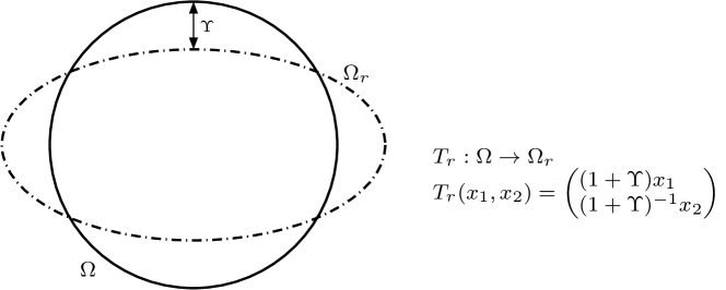
Figure 4: Illustration of an example for the application of Corollary 1.

We conclude by discussing a simple application of this corollary. Figure 4 illustrates the setting. Let $\Omega$ be the unit sphere, $\Omega_{r}$ be an ellipse

$$\Omega=\{x\in\mathds{R}^{2}\,:\,x_{1}^{2}+x_{2}^{2}<1\},\quad\Omega_{r}=\{x\in\mathds{R}^{2}\,:\,(1+\Upsilon)^{2}x_{1}^{2}+(1+\Upsilon)^{-2}x_{2}^{2}<1\}.$$

It holds $\operatorname{dist}(\partial\Omega,\partial\Omega_{r})\leq\Upsilon$ and we define the map $T_{r}:\Omega\to\Omega_{r}$ by

$$T_{r}(x)=\begin{pmatrix}(1+\Upsilon)^{-1}x_{1}\\ (1+\Upsilon)x_{2},\end{pmatrix},\quad F_{r}=\nabla T_{r}=\begin{pmatrix}(1+\Upsilon)^{-1}&0\\ 0&(1+\Upsilon)\end{pmatrix},\quad J_{r}=1.$$

This map satisfies the assumptions of the corollary

$$I-J_{r}F_{r}^{-1}F_{r}^{-T}=\Upsilon(\Upsilon+2)\begin{pmatrix}-1&0\\ 0&(1+\Upsilon)^{-2}\end{pmatrix},\quad\|I-J_{r}F_{r}^{-1}F_{r}^{-T}\|_{\infty}=2\Upsilon+\Upsilon^{2}.$$

4 Numerical illustration

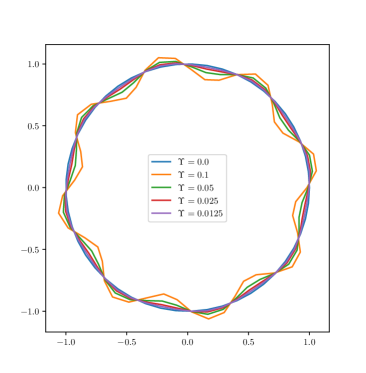
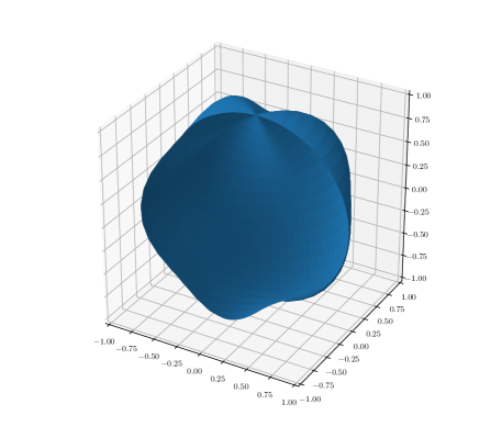
Figure 5: Sketch of the computational domains w.r.t. the parameter $\Upsilon$ in two dimensions (left) and for $\Upsilon=0.1$ in three dimensions (right).

In this section we illustrate the theoretical results from the previous section. We compute the Laplace problem on a family of domains representing different values of $\Upsilon$. Moreover, we numerically extend the analytical predictions and show that a similar behavior holds for the Stokes system.

We consider $\Omega$ to be a unit ball in two and three dimensions and define a family of perturbed domains $\Omega_{\Upsilon}$, with the amplitude of the perturbation being dependent on the coefficient $\Upsilon$, cf. Figure 5.

In two dimensions, the boundary of the domain $\Omega_{\Upsilon}$ is given in polar coordinates $(\rho,\varphi)$ by

$$\partial\Omega_{\Upsilon}=\{(1-\Upsilon/5+\Upsilon\sin(8\varphi),\varphi)\text{ for }\varphi\in[0,2\pi)\},$$

and in three dimensions in spherical coordinates $(\rho,\theta,\varphi)$ by

$$\partial\Omega_{\Upsilon}=\{(1-\Upsilon/5+\Upsilon\sin(3\varphi)\sin(3\theta),\theta,\varphi)\text{ for }\theta\in[0,\pi),\varphi\in[0,2\pi)\}.$$

For computations we take

$$\Upsilon\in\{0,0.0125,0.025,0.05,0.1\}.$$

In order to illustrate the convergence result from Theorem 3.2, we compute the model problem on a series of uniformly refined meshes. The dependence between the mesh size $h$ and the refinement level $L$ reads $h=2^{-L}$. We denote the mesh approximating $\Omega_{\Upsilon}$, with a mesh size $h$, by $\Omega_{h,\Upsilon}$.

The numerical implementation is realized in the software library Gascoigne 3D Gascoigne3d , using iso-parametric finite elements of degree $1$ and $2$. A detailed description of the underlying numerical methods is given in Richter2017 .

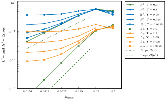
Figure 6: $L^{2}$- and $H^{1}$-errors w.r.t. mesh-size $h_{max}$ for varying parameter $\Upsilon$ computed for the Laplace problem in three-dimensions with linear finite elements.

4.1 Laplace equation in two and three dimensions

We consider the following problem

$$-\Delta u=f\text{ in }\Omega,\quad u=0\text{ on }\partial\Omega,$$ (37)

where $\Omega$ is the unit ball in two dimensions and the unit sphere in three dimensions.

To compute errors we choose a rotationally symmetric analytical solution to (37) as

$$u(r)=-\cos\left(\frac{\pi}{2}r\right)$$

with $r=\sqrt{x^{2}+y^{2}}$ in two and $r=\sqrt{x^{2}+y^{2}+z^{2}}$ in three dimensions, respectively, which results in the right hand sides

$$f_{2d}(r)=\frac{\pi}{2r}\sin\left(\frac{\pi}{2}r\right)+\frac{\pi^{2}}{4}\cos\left(\frac{\pi}{2}r\right),\quad f_{3d}(r)=\frac{\pi}{r}\sin\left(\frac{\pi}{2}r\right)+\frac{\pi^{2}}{4}\cos\left(\frac{\pi}{2}r\right).$$

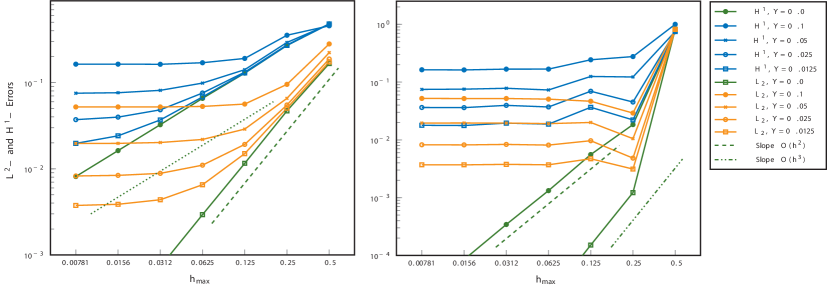
Figure 7: $L^{2}$- and $H^{1}$-errors w.r.t. mesh-size $h_{max}$ for varying parameter $\Upsilon$ computed for the Laplace problem in two-dimensions with FE. Left: linear finite elements. Right: quadratic finite elements.

For the ease of evaluations the errors, the $H^{1}$- and $L^{2}$-norms will be computed on the truncated domains

$$\Omega^{\prime}_{2d} =\{(\varphi,\rho)\text{ for }\varphi\in[0,2\pi)\text{ and }\rho\in(0,0.88)\},$$

$$\Omega^{\prime}_{3d} =\{(\varphi,\theta,\rho)\text{ for }\theta\in[0,\pi),\varphi\in[0,2\pi)\text{ and }\rho\in(0,0.88)\},$$

see also Remark 4. We hence do not compute the errors $\|\nabla(u-u_{h})\|$ and $\|u-u_{h}\|$ on the remainders $\Omega\setminus\Omega_{r}$. Therefore we expect optimal order convergence in the spirit of Corollary 1. The restriction of the domain to an area within $\Omega_{h}$ is also by technical reasons, as the evaluation of integrals outside of the meshed area is not easily possible.

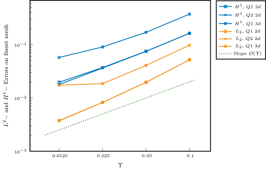
Figure 8: $L^{2}$- and $H^{1}$-errors w.r.t. parameter $\Upsilon$ computed for the Laplace problem in two and three-dimensions with linear and quadratic finite elements.

In Figures 6 and 7 we see the resulting $L^{2}$- and $H^{1}$-errors. We observe that for finer meshes, $\Upsilon$ becomes the dominating factor of the error. In particular the use of quadratic finite elements shows a strong imbalance between FE error and geometric error, which quickly dominates as seen in the left part of Fig. 7. The result is consistent with Corollary 1. As soon as the FE error is smaller than the geometry perturbation $\Upsilon$, we do not observe any further improvement of the error. In Fig. 8 we show the convergence in both norms in terms of the geometry parameter $\Upsilon$. Linear convergence is clearly observed. The apparent decay of convergence rate in case of the $L^{2}$-error in three dimensions is due to the still dominating FE error in this case.

4.2 Stokes system in two dimensions

To go beyond the Laplace problem, we investigate the behavior of the solution to the Stokes system with respect to the domain variation in two spatial dimensions. The problem is to find the velocity u and the pressure $p$ such that

$$\operatorname{div}\,\textbf{u}=0,\quad-\Delta\textbf{u}+\nabla p=\textbf{f}\text{ in }\Omega,$$ (38)

with homogeneous Dirichlet condition $\textbf{u}=0$ on the boundary $\partial\Omega$ and a right hand side vector f. System (38) is solved with equal-order iso-parametric finite elements using pressure stabilization by local projections, see BeckerBraack2001 .

We prescribe an analytical solution for comparison with the finite element approximation

$$\textbf{u}(x,y)=\cos\left(\frac{\pi}{2}(x^{2}+y^{2})\right)\begin{pmatrix}y\\ -x\end{pmatrix},$$

where the corresponding forcing term reads

$$\textbf{f}(x,y)=\pi\cos\left(\frac{\pi}{2}(x^{2}+y^{2})\right)\begin{pmatrix}yr^{2}\pi+4(y-x)\tan\left(\frac{\pi}{2}(x^{2}+y^{2})\right)\\ -xr^{2}\pi-4(x+y)\tan\left(\frac{\pi}{2}(x^{2}+y^{2})\right)\end{pmatrix}.$$

In Figure 9 we see the resulting $L^{2}$- and $H^{1}$-errors. Again we observe that $\Upsilon$ becomes the dominant factor for finer meshes. This result is not covered by the theoretical findings, however it shows that geometric uncertainty should be taken into account for the simulations of flow models.

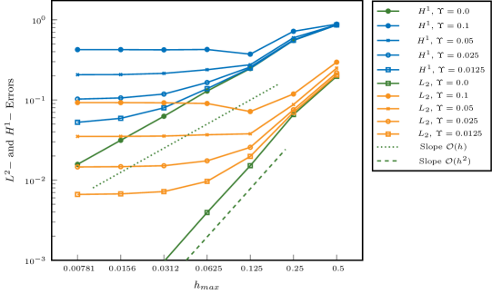
Figure 9: $L^{2}$- and $H^{1}$-errors w.r.t. mesh-size $h_{max}$ for varying parameter $\Upsilon$ computed for the Stokes problem in two dimensions with linear finite elements.

5 Conclusions

We have demonstrated that small boundary variations have crucial impact on the result of the finite element simulations. The developed error estimates are linear with respect to the maximal distance $\Upsilon$ between the real and the approximated domains, cf. Theorem 3.2. We have illustrated the sharp nature of this bound in the computations performed in Section 4.

Particularly, in the case of first and second order approximation we observe how the relation between the mesh size $h$ and aforementioned $\Upsilon$ impact the resulting $L^{2}$- and $H^{1}$-errors. The same behavior has been demonstrated numerically for the Stokes system.

In practice we do not have control on the accuracy of the domain reconstruction. This has shown that it is worth to take into account the geometric uncertainty when deciding on the mesh-size in order to avoid unnecessary computational effort.

In this work we have focused on the Laplace problem (2). Additionally, the Stokes system has been treated numerically and it exhibits similar features. In future work we will extend this consideration to flow models, in particular the Navier-Stokes equations MiMiRi2019 . Among the additional challenges in extending the present work to the Navier-Stokes system are the consideration of the typical saddle-point structure of incompressible flow models introducing a pressure variable RannacherRichter2018 and the difficulty of nonlinearities introduced by the convective term, and thus the non-uniqueness of solutions HeywoodRannacher1990 .

- (1) G. Allaire and C. Dapogny. A deterministic approximation method in shape optimization under random uncertainties. Journal of computational mathematics, 1:83–143, 2015.
- (2) I. Babuška and J. Chleboun. Effects of uncertainties in the domain on the solution of neumann boundary value problems in two spatial dimensions. Mathematics of Computation, 71(240):1339–1370, 2002.
- (3) I. Babuška and J. Chleboun. Effects of uncertainties in the domain on the solution of dirichlet boundary value problems. Numerische Mathematik, 93(4):583–610, 2003.
- (4) Gabriel R. Barrenechea and Cheherazada González. A stabilized finite element method for a fictitious domain problem allowing small inclusions. Numerical Methods for Partial Differential Equations, 34(1):167–183, August 2017.
- (5) R. Becker and M. Braack. A finite element pressure gradient stabilization for the Stokes equations based on local projections. Calcolo, 38(4):173–199, 2001.
- (6) R. Becker, M. Braack, D. Meidner, T. Richter, and B. Vexler. The finite element toolkit Gascoigne. http://www.gascoigne.de.
- (7) C. Bernardi. Optimal finite-element interpolation on curved domains. SIAM Journal on Numerical Analysis, 26(5):1212–1240, 1989.
- (8) A.-P. Calderón. Lebesgue spaces of differentiable functions and distributions. In Proc. Sympos. Pure Math., volume IV, pages 33–49. AMS, 1961.
- (9) Andrea Cangiani, Emmanuil H. Georgoulis, and Younis A. Sabawi. Adaptive discontinuous galerkin methods for elliptic interface problems. Mathematics of Computation, 87(314):2675–2707, February 2018.
- (10) C. Canuto and T. Kozubek. A fictitious domain approach to the numerical solution of pdes in stochastic domains. Numerische Mathematik, 107(2):257, 2007.
- (11) P.G. Ciarlet. The Finite Element Method for Elliptic Problems, volume 40 of Classics. SIAM, 2002.
- (12) M. Dambrine, H. Harbrecht, and B. Puig. Computing quantities of interest for random domains with second order shape sensitivity analysis. ESAIM: Mathematical Modelling and Numerical Analysis, 49(5):1285–1302, August 2015.
- (13) M. D’Elia, L. Mirabella, T. Passerini, M. Perego, M. Piccinelli, C. Vergara, and A. Veneziani. Applications of variational data assimilation in computational hemodynamics, pages 363–394. Springer Milan, Milano, 2012.
- (14) I. Ergatoudis, B.M. Irons, and O.C. Zienkiewicz. Curved, isoparametric “quadrilateral” elements for finite element analysis. I. J. of Solids and Structures, 4(1):31–42, 1968.
- (15) A. Ern and J.-L. Guermond. Theory and Practice of Finite Elements. Applied Mathematical Sciences, 159, Springer, 2004.
- (16) L.C. Evans. Partial differential equations. American Mathematical Society, Providence, R.I., 2010.
- (17) S.W. Funke, M. Nordaas, O. Evju, M.S. Alnaes, and K.A. Mardal. Variational data assimilation for transient blood flow simulations: Cerebral aneurysms as an illustrative example. International Journal for Numerical Methods in Biomedical Engineering, 35(1):e3152, 2019. e3152 cnm.3152.
- (18) H. Harbrecht, M. Peters, and M. Siebenmorgen. Analysis of the domain mapping method for elliptic diffusion problems on random domains. Numerische Mathematik, 134(4):823–856, 2016.
- (19) H. Harbrecht, R. Schneider, and C. Schwab. Sparse second moment analysis for elliptic problems in stochastic domains. Numerische Mathematik, 109(3):385–414, 2008.
- (20) J. Heywood and R. Rannacher. Finite element approximation of the nonstationary Navier-Stokes problem. IV. Error analysis for second-order time discretization. SIAM Journal on Numerical Analysis, 27(3):353–384, 1990.
- (21) M. Lenoir. Optimal isoparametric finite elements and error estimates for domains involving curved boundaries. SIAM Journal on Numerical Analysis, 23(3):562–580, 1986.
- (22) P. Minakowski, J. Mizerski, and T. Richter. Variablity of clinical hemodynamical factors under geometric uncertainty. in preparation, 2019.
- (23) J. A. Moore, D. A. Steinman, D. W. Holdsworth, and C. R. Ethier. Accuracy of computational hemodynamics in complex arterial geometries reconstructed from magnetic resonance imaging. Annals of Biomedical Engineering, 27(1):32–41, 1999.
- (24) J.A. Moore, D.A. Steinman, and C.R. Ethier. Computational blood flow modelling: Errors associated with reconstructing finite element models from magnetic resonance images. Journal of Biomechanics, 31(2):179 – 184, 1997.
- (25) D. Nolte and C. Bertoglio. Reducing the impact of geometric errors in flow computations using velocity measurements. International Journal for Numerical Methods in Biomedical Engineering, page e3203, April 2019.
- (26) W.L. Oberkampf and M.F. Barone. Measures of agreement between computation and experiment: Validation metrics. Journal of Computational Physics, 217(1):5–36, September 2006.
- (27) W.L. Oberkampf and C.J. Roy. Verification and Validation in Scientific Computing. Cambridge University Press, 2010.
- (28) D.A. Di Pietro and A. Ern. Mathematical Aspects of Discontinuous Galerkin Methods. Springer Berlin Heidelberg, 2012.
- (29) A. Quarteroni, M. Tuveri, and A. Veneziani. Computational vascular fluid dynamics: problems, models and methods. Computing and Visualization in Science, 2(4):163–197, 2000.
- (30) R. Rannacher and T. Richter. A priori estimates for the Stokes equations with slip boundary conditions on curved domains. in preparation, 2019.
- (31) T. Richter. Fluid-structure Interactions. Models, Analysis and Finite Elements, volume 118 of Lecture notes in computational science and engineering. Springer, 2017.
- (32) D.M. Tartakovsky and D. Xiu. Stochastic analysis of transport in tubes with rough walls. Journal of Computational Physics, 217(1):248 – 259, 2006.
- (33) D. Xiu and D. Tartakovsky. Numerical methods for differential equations in random domains. SIAM Journal on Scientific Computing, 28(3):1167–1185, 2006.
- (34) G. Xu, B. Mourrain, R. Duvigneau, and A. Galligo. Parameterization of computational domain in isogeometric analysis: Methods and comparison. Computer Methods in Applied Mechanics and Engineering, 200(23):2021 – 2031, 2011.
- (35) G. Xu, B. Mourrain, R. Duvigneau, and A. Galligo. Constructing analysis-suitable parameterization of computational domain from cad boundary by variational harmonic method. Journal of Computational Physics, 252:275 – 289, 2013.