Adaptive scale-invariant online algorithms for learning linear models

Abstract

We consider online learning with linear models, where the algorithm predicts on sequentially revealed instances (feature vectors), and is compared against the best linear function (comparator) in hindsight. Popular algorithms in this framework, such as Online Gradient Descent (OGD), have parameters (learning rates), which ideally should be tuned based on the scales of the features and the optimal comparator, but these quantities only become available at the end of the learning process. In this paper, we resolve the tuning problem by proposing online algorithms making predictions which are invariant under arbitrary rescaling of the features. The algorithms have no parameters to tune, do not require any prior knowledge on the scale of the instances or the comparator, and achieve regret bounds matching (up to a logarithmic factor) that of OGD with optimally tuned separate learning rates per dimension, while retaining comparable runtime performance.

1 Introduction

We consider the problem of online learning with linear models, in which at each trial $t=1,\ldots,T$, the algorithm receives an input instance (feature vector) $\bm{x}_{t}\in\mathbb{R}^{d}$, upon which it predicts $\widehat{y}_{t}\in\mathbb{R}$. Then, the true label $y_{t}$ is revealed and the algorithm suffers loss $\ell(y_{t},\widehat{y}_{t})$, convex in $\widehat{y}_{t}$. The goal of the algorithm is have its cumulative loss not much larger to that of any linear predictor of the form $\bm{x}\mapsto\bm{x}^{\top}\bm{u}$ for $\bm{u}\in\mathbb{R}^{d}$, i.e. to have small regret against any comparator $\bm{u}$. This problem encompasses linear regression and classification (with convex surrogate losses) and has been extensively studied in numerous past works (Littlestone et al., 1991; Cesa-Bianchi et al., 1996; Shalev-Shwartz, 2011; Hazan, 2015).

One of the most popular algorithms in this framework is Online Gradient Descent (OGD) (Cesa-Bianchi et al., 1996). Its predictions are given by $\widehat{y}_{t}=\bm{x}_{t}^{\top}\bm{w}_{t}$ for a weight vector $\bm{w}_{t}\in\mathbb{R}^{d}$ updated using a simple rule

$$\bm{w}_{t+1}=\bm{w}_{t}-\eta\nabla_{t},$$ (1)

where $\nabla_{t}$ is a (sub)gradient of the loss $\ell(y_{t},\widehat{y}_{t})$ at $\bm{w}_{t}$, and $\eta$ is a parameter of the algorithm, called the learning rate. With the optimal “oracle” tuning of $\eta$ (which involves the norm of the comparator $\bm{u}$ and of the observed gradients, unknown to the algorithm in advance), OGD would achieve a bound on the regret against $\bm{u}$ of order $\|\bm{u}\|\sqrt{\sum_{t}\|\nabla_{t}\|^{2}}$ (Zinkevich, 2003). Unfortunately, this bound might be very poor if the features have distinct scales. To see that first note that $\nabla_{t}$ is proportional to $\bm{x}_{t}$ due to linear dependence of $\widehat{y}_{t}$ on $\bm{x}_{t}$. Now, let $\bm{u}$ be the comparator which minimizes the total loss (assume such exists). If we scale the first coordinate of each $\bm{x}_{t}$ by a factor of $c$, the first coordinate of the optimal comparator $\bm{u}$ will scale down by a factor of $c^{-1}$, so its prediction and (optimal) loss remain the same, and the bound above will in general become worse by a factor of $\max\{c,c^{-1}\}$ (Ross et al., 2013). This is a well known issue with gradient descent, and is usually solved by prior normalization of the features. However, such pre-processing step cannot be done in an online setting.

The problem described above becomes apparent if we make an analogy from physics and imagine that all features have physical units. In particular, if we assigned a unit $\bm{[}x_{i}\bm{]}$ to feature $i$, and assumed for simplicity that the prediction and the label are unitless (as in, e.g., classification), the corresponding coordinate of the weight vector would need to have unit $1/\bm{[}x_{i}\bm{]}$. However, the units in the OGD update (1) are mismatched, because $\nabla_{t,i}$ has unit $\bm{[}x_{i}\bm{]}$ (as $\nabla_{t}$ is proportional to $\bm{x}_{t}$), while $w_{t,i}$ has unit $1/\bm{[}x_{i}\bm{]}$; even assigning a unit to $\eta$ does not help as a single number cannot compensate different units. A reasonable solution to this “unit clash” problem is to use one learning rate per dimension, i.e. to modify (1) to:

$$w_{t+1,i}=w_{t,i}-\eta_{i}\nabla_{t,i},\qquad i=1,\ldots,d.$$ (2)

If we choose the oracle tuning of the learning rates to minimize the regret against comparator $\bm{u}$, it follows that $\eta_{i}^{*}=|u_{i}|/\sqrt{\sum_{t}\nabla_{t,i}^{2}}$ which results in the regret bound of order $\sum_{i}|u_{i}|\sqrt{\sum_{t}\nabla_{t,i}^{2}}$, better than the bound obtained with a single learning rate. Interestingly, the unit of $\eta_{i}^{*}$ becomes $1/[x_{i}]^{2}$, which fixes the “unit clash” in (2) and makes the scaling issues go away (as now scaling the $i$-the feature by any factor $c$ will be compensated by scaling down $u_{i}$ by $c^{-1}$). Unfortunately, it is infeasible in practice to separately tune a single learning rate per dimension (oracle tuning requires the knowledge the comparator and all future gradients).

Our contribution.

In this paper we provide adaptive online algorithms which for any comparator $\bm{u}$ achieve regret bounds matching, up to logarithmic factors, that of OGD with optimally tuned separate learning rates per dimension. Note that as we want to capture arbitrary feature scales and comparators, our bounds come without any prior assumptions on the magnitude of instances $\bm{x}_{t}$, comparator $\bm{u}$, or even predictions $\bm{x}_{t}^{\top}\bm{u}$, as has been commonly assumed in the past work (we do, however, assume the Lipschitzness of the loss with respect to the prediction, which is satisfied for various popular loss functions, such as logistic, hinge or absolute losses). Our algorithms achieve their bounds without the need to tune any hyperparameters, and have runtime performance of $O(d)$ per iteration, which is the same as that of OGD. As a by-product of being adaptive to the scales of the instances and the comparator, the proposed algorithms are scale-invariant: their predictions are invariant under arbitrary rescaling of individual features (Ross et al., 2013). More precisely, after multiplying the $i$-th coordinate of all input instances by a fix scaling factor $a_{i}$, $x_{t,i}\mapsto a_{i}x_{t,i}$ for all $t$, the predictions of the algorithms remain the same: they are independent on the units in which the instance vectors are expressed (in particular, they do do not require any prior normalization of the data). To achieve our goals, the design of our algorithms heavily rely on techniques recently developed in adaptive online learning (Streeter & McMahan, 2012; Orabona & Pál, 2016; Cutkosky & Boahen, 2017; Cutkosky & Orabona, 2018).

The first algorithm achieves a regret bound which depends on instances only relative to the scale of the comparator, through products of the form $|u|_{i}\sqrt{\max_{t}|x_{t,i}|^{2}+\sum_{t}\nabla_{t,i}^{2}}$ for $i=1,\ldots,d$, similarly as in the bound of OGD with per-dimension learning rates (with additional maximum over feature values, which is usually much smaller than the sum over squared gradients). As the algorithm can be sometimes a bit conservative in its predictions, we also introduce a second algorithm which is more aggressive in decreasing its cumulative loss; the price to pay is a regret bound which mildly (logarithmically) depends on ratios between the largest and the first non-zero input value for each coordinate. While these quantities can be made arbitrarily large in the worst case, it is unlikely to happen in practice. We test both algorithms in a computational study on several real-life data sets and show that without any need to tune parameters, they are competitive to popular online learning methods, which are allowed to tune their learning rates to optimize the test set performance.

Related work.

Our work is rooted from a long line of research on regret minimizing online algorithms (Cesa-Bianchi et al., 1996; Kivinen & Warmuth, 1997; Cesa-Bianchi & Lugosi, 2006). Most of the proposed methods have “range factors” present both in the algorithm and in the bound: it is typically assumed that some prior knowledge on the range of the comparator and the gradients is given, which allows the algorithm to tune its parameters appropriately. For instance, assuming $\|\bm{u}\|\leq U$ and $\|\nabla_{t}\|\leq G$ for all $t$, OGD (1) with learning rate $\eta=U/(G\sqrt{T})$ achieves $O(UG\sqrt{T})$ regret bound.

More recent work on adaptive algorithms aims to get rid of these range factors. In particular, with a prior bound on the comparator norm, it is possible to adapt to the unknown range of the gradients (Duchi et al., 2011; Orabona & Pál, 2015), whereas having a prior bound on all future gradients, one can adapt to the unknown norm of the comparator (Streeter & McMahan, 2012; McMahan & Abernethy, 2013; Orabona, 2014; Orabona & Pál, 2016; Orabona & Tommasi, 2017; Cutkosky & Orabona, 2018). In particular, using reduction methods proposed by Cutkosky & Orabona (2018), one can get a bound matching OGD with separate learning rate per dimension, but this requires to know $\max_{t,i}|\nabla_{t,i}|$ in advance. Interestingly, Cutkosky & Boahen (2017) have shown that in online convex optimization it is not possible to adapt to both unknown gradient range and unknown comparator norm at the same time. Here, we circumvent this negative result by exploiting the fact that the input instance $\bm{x}_{t}$ is available ahead of prediction and therefore can be used to construct $\widehat{y}_{t}$ (this idea was first discovered in the context of linear regression (Vovk, 2001; Azoury & Warmuth, 2001)).

Scale-invariant algorithm has been been studied by Ross et al. (2013); Orabona et al. (2015) in a setup very similar to ours. Their algorithms, however, require a prior knowledge on the largest per-coordinate comparator’s prediction, $\max_{t,i}|u_{i}x_{t,i}|$, whereas their bounds scale with relative ratios between the largest and the first non-zero input value for each coordinate (the bound of our second algorithm also depends on these quantities but only in a logarithmic way). Luo et al. (2016); Koren & Livni (2017) considered even a more general setup of invariance under linear transformation of features (of which our invariance is a special case if the transformation is diagonal), but a prior knowledge of $\max_{t}|\bm{x}_{t}^{\top}\bm{u}|$ must be available, and the resulting algorithms are second-order methods. The closest to our work are the results by Kotłowski (2017), which concern the same setup, general invariance under linear transformations, and, similarly to us, make no prior range assumptions. Their bounds, however, do not scale with gradients $\nabla_{t,i}^{2}$ (as in the optimal OGD bound), but with the size of the features $x_{t,i}^{2}$ (multiplied by the Lipschitz constant of the loss), which upper-bounds $\nabla_{t,i}^{2}$ and can become much larger. For instance, in the “noise-free” case, when some comparator $\bm{u}$ has zero loss, the algorithm playing sufficiently close to $\bm{u}$ can inflict arbitrarily small gradients, while the sum of squared feature values will still grow linearly in $t$.

The goal of scale-invariance seems to go hand in hand with a requirement for the updates to avoid unit clashes and this connection was the motivating idea for our work. In the most basic case, assume you want to design online algorithms for linear regression

$$\bm{w}_{t+1}=\bm{w}_{t}-\eta(\bm{x}_{t}^{\top}\bm{w}_{t}-y_{t})\bm{x}_{t}$$

that are to be robust to scaling the input vectors $\bm{x}_{t}$ by a single positive constant factor. In this case $\bm{[}\eta\bm{]}$ should be $1/\bm{[}\|\bm{x}_{t}\|^{2}\bm{]}$. Interestingly enough, good tunings of the learning rates $\eta$ often “fix the units”: the properly tuned learning rates for the linear regression updates employed in (Cesa-Bianchi et al., 1996; Kivinen & Warmuth, 1997) have units $1/\bm{[}\|\bm{x}_{t}\|^{2}\bm{]}$. In this paper we focus on robustness to independently scaling the individual components $x_{t,i}$ of the input vectors by positive factors. This requires privatized learning rates $\eta_{i}$ with the property that $\bm{[}\eta_{i}\bm{]}=1/\bm{[}x_{t,i}\bm{]}^{2}$. Our paper focuses on this case because of efficiency concerns. However there is a third case (more expensive) where we want robustness to independent scaling and rotation of the input vectors $\bm{x}_{t}$. Now $\bm{\eta}$ must be a matrix parameter (playing a similar role to a Hessian) and if the instances are pre-multiplied by a fixed invertible $\bm{A}$, then the tuned learning rate matrix of the new instances must become $\bm{\eta}\bm{A}^{-1}$, thus correcting for the pre-multiplication with $\bm{A}$. The updates of Luo et al. (2016); Koren & Livni (2017); Kotłowski (2017), as well as the Newton algorithm, have this form, but they are all second order algorithms with runtime of at least $O(d^{2})$ per trial.

2 Problem Setting

Our online learning protocol is defined as follows. In each trial $t=1,\ldots,T$, the algorithm receives an input instance $\bm{x}_{t}\in\mathbb{R}^{d}$, on which it predicts $\widehat{y}_{t}\in\mathbb{R}$; we will always assume linear predictions $\widehat{y}_{t}=\bm{x}_{t}^{\top}\bm{w}_{t}$, where $\bm{w}_{t}\in\mathbb{R}^{d}$ is allowed to depend on $\bm{x}_{t}$. Then, the output label $y_{t}\in\mathcal{Y}$ is revealed, and the algorithm suffers loss $\ell(y_{t},\widehat{y}_{t})$. As we make no assumptions about the label set $\mathcal{Y}$, in what follows we incorporate $y_{t}$ into the loss function and use $\ell_{t}(\widehat{y})$ to denote $\ell(y_{t},\widehat{y})$. The performance of the algorithm is measured by means of the regret:

$$R_{T}(\bm{u})=\sum_{t=1}^{T}\ell_{t}(\bm{x}_{t}^{\top}\bm{w}_{t})-\sum_{t=1}^{T}\ell_{t}(\bm{x}_{t}^{\top}\bm{u}),$$

which is the difference between the cumulative loss of the algorithm and that of a fixed, arbitrarily chosen, comparator weight vector $\bm{u}\in\mathbb{R}^{d}$ (for instance, $\bm{u}$ can be the minimizer of the cumulative loss on the whole data sequence, if such exists).

Loss function	$\ell(y,\widehat{y})$	$\partial_{\widehat{y}}\ell(y,\widehat{y})$	$L$
logistic	$\ln\left(1+e^{-y\widehat{y}}\right)$	$\frac{-y}{1+e^{y\widehat{y}}}$	1
hinge	$\max\{0,1-y\widehat{y}\}$	$-y\bm{1}[y\widehat{y}\leq 1]$	1
absolute	$|\widehat{y}-y|$	$\mathrm{sgn}(\widehat{y}-y)$	1

Table 1: $L$-Lipschitz loss functions for classification and regression. $\bm{1}[\cdot]$ denotes an indicator function.

We assume that for any $t$, $\ell_{t}(\widehat{y})$ is convex and $L$-Lipschitz; the latter implies that the (sub)derivative of the loss is bounded, $|\partial\ell_{t}(\widehat{y})|\leq L$. Table 1 lists three popular losses with these properties. Throughout the paper, we assume $L=1$ without loss of generality. Our setup can be considered as a variant of online convex optimization (Shalev-Shwartz, 2011; Hazan, 2015), with the main difference in $\bm{x}_{t}$ being observed before prediction.

We use a standard argument exploiting the convexity of the loss to bound $\ell_{t}(\widehat{y}^{\prime})\geq\ell_{t}(\widehat{y})+\partial\ell_{t}(\widehat{y})(\widehat{y}^{\prime}-\widehat{y})$ for any $\widehat{y},\widehat{y}^{\prime}\in\mathbb{R}$. Substituting $\widehat{y}=\bm{w}_{t}^{\top}\bm{x}_{t}$ and $\widehat{y}^{\prime}=\bm{u}^{\top}\bm{x}_{t}$, and denoting $g_{t}=\partial\ell_{t}(\widehat{y}_{t})\in[-1,1]$ for each $t$, the regret is upper-bounded by:

$$R_{T}(\bm{u})\leq\sum_{t=1}^{T}g_{t}\bm{x}_{t}^{\top}(\bm{w}_{t}-\bm{u}),$$ (3)

where $|g_{t}|\leq 1$ follows from the Lipschitzness of the loss. Note that $g_{t}\bm{x}_{t}$ is equal to $\nabla_{t}=\nabla_{\bm{w}_{t}}\ell_{t}(\bm{x}_{t}^{\top}\bm{w}_{t})$, the (sub)gradient of the loss with respect to the weight vector $\bm{w}_{t}$. Thus, we can bound the regret with respect to the original convex loss $\ell_{t}(\bm{x}_{t}^{\top}\bm{w})$ by upper-bounding its linearized version $g_{t}\bm{x}_{t}^{\top}\bm{w}$ on the right-hand side of (3).

Consider running Online Gradient Descent (OGD) algorithm on this problem, as defined in (2), i.e. we let the algorithm have a separate learning rate per dimension. When initialized at $\bm{w}_{1}=\bm{0}$, OGD achieves the regret bound:

$$R_{T}(\bm{u})\leavevmode\nobreak\ \leq\leavevmode\nobreak\ \sum_{i=1}^{d}\left(\frac{u_{i}^{2}}{2\eta_{i}}+\frac{\eta_{i}}{2}S^{2}_{T,i}\right),$$

where we introduced $S^{2}_{t,i}=\sum_{j\leq t}\nabla_{j,i}^{2}=\sum_{j\leq t}(g_{j}x_{j,i})^{2}$. This is a slight generalization of a standard textbook bound (see, e.g., Hazan, 2015), proven in Appendix A for completeness. Tuning the learning rates to minimize the bound results in $\eta_{i}=\frac{|u_{i}|}{S_{t,i}}$, and the bound simply becomes:

$$R_{T}(\bm{u})\leq\sum_{i=1}^{d}|u_{i}|S_{T,i}.$$ (4)

Such tuning is, however, not directly feasible as it would require knowing the comparator and the future gradients in hindsight. The goal of this work is to design adaptive online algorithms which for any comparator $\bm{u}$, and any data sequence $\{(\bm{x}_{t},y_{t})\}_{t=1}^{T}$, without any prior knowledge on their magnitudes, achieve (4) up to logarithmic factors.

An interesting property of bound (4) is that it captures a natural symmetry of our linear framework. Given a data sequence, let $\bm{u}$ be the minimizer of the cumulative loss, $\bm{u}=\operatorname*{argmin}_{\bm{w}}\sum_{t}\ell_{t}(\bm{x}_{t}^{\top}\bm{w})$ (assume such exists). If we apply a coordinate-wise transformation $x_{t,i}\mapsto a_{i}x_{t,i}$ simultaneously to all input instances ($t=1,\ldots,T$) for any positive scaling factors $a_{1},\ldots,a_{d}$, the minimizer of the loss will undergo the inverse transformation $u_{i}\mapsto a_{i}^{-1}u_{i}$ to keep its predictions $\bm{x}_{t}^{\top}\bm{u}$, and thus its cumulative loss, invariant. Indeed, $\bm{u}$ minimizes $\sum_{t}\ell_{t}(\bm{x}_{t}^{\top}\bm{w})$ if and only if $\bm{A}^{-1}\bm{u}$ minimizes $\sum_{t}\ell_{t}((\bm{A}\bm{x}_{t})^{\top}\bm{w})$ for $\bm{A}=\mathrm{diag}(a_{1},\ldots,a_{d})$. Thus, when (4) is evaluated at the loss minimizer, it becomes invariant under any such scale transformation.

The invariance of predictions of the optimal comparator leads to the definition of scale-invariant algorithms. We call a learning algorithm scale-invariant if its behavior (sequence of predictions) is invariant under arbitrary rescaling of individual features (Ross et al., 2013; Kotłowski, 2017). More precisely, if we apply a transformation $x_{t,i}\mapsto a_{i}x_{t,i}$ simultaneously to all instances, the predictions of the algorithm $\widehat{y}_{1},\ldots,\widehat{y}_{T}$ remain the same as on the original data sequence. Scale-invariant algorithm are thus independent on the “units” in which the instance vectors are expressed on each feature, and do not require any prior normalization of the data. Interestingly, OGD defined in (2) is not a scale invariant algorithm, but becomes one under the optimal tuning of its learning rates. The algorithms presented in the next section will turn out to be scale-invariant, essentially as a by-product of adaptiveness to arbitrary scale of the comparator and the instances, required to achieve (4).

Remark: As noted in the introduction, scale invariance can be generalized to arbitrary linear invertible transformations $\bm{x}_{t}\mapsto\bm{A}\bm{x}_{t}$. Unfortunately, this leads to second-order algorithms (Luo et al., 2016; Koren & Livni, 2017; Kotłowski, 2017), with the complexity at least $\Theta(d^{2})$ per trial.

3 Scale-invariant algorithms

Motivation.

We first briefly describe the motivating idea behind the construction of the algorithms. We start with rewriting the right hand side of (3) to get:

$$R_{T}(\bm{u})\leq\sum_{i=1}^{d}\Big{(}\underbrace{\sum_{t=1}^{T}g_{t}x_{t,i}(w_{t,i}-u_{i})}_{\stackrel{{\scriptstyle def}}{{=}}\tilde{R}_{T,i}(u_{i})}\Big{)},$$

so that it decouples coordinate-wise and it suffices to separately bound each term $\tilde{R}_{T,i}(u_{i})$ $i=1,\ldots,d$. As we aim to get close to (4), we want for each $i$ a bound of the form $\tilde{R}_{T,i}(u_{i})\leq B(u_{i}S_{T,i})+c_{T}$, for some function $B(\cdot)$ plus a potential additional overhead $c_{T}$ (to exactly get (4) we could set $B(x)=|x|$ and $c_{T}=0$, but this turns out to be unachievable without any prior knowledge on the comparator). Using $G_{t,i}=-\sum_{j\leq t}g_{j}x_{j,i}$ to denote the cumulative negative gradient coordinate, such bound can be equivalently written as:

$$\sum_{t=1}^{T}g_{t}x_{t,i}w_{t,i}+G_{T,i}u_{i}-B(u_{i}S_{T,i})\leq c_{T}.$$

Now, the key idea is to note that the bound must hold for any comparator $u_{i}$, therefore it must hold if we take a supremum over $u_{i}$ on the left-hand side, $\sup_{u_{i}}\{G_{T,i}u_{i}-B(u_{i}S_{T,i})\}$. To evaluate this supremum, we note that under variable change $x=u_{i}S_{T,i}$ it becomes equivalent to $\sup_{x}\{G_{T,i}/S_{T,i}x-B(x)\}$. Recalling the definition of the Fenchel conjugate of a function $f(x)$, defined as $f^{*}(\theta)=\sup_{x}\{\theta x-f(x)\}$ (Boyd & Vandenberghe, 2004), we see that the supremum can be evaluated to $B^{*}(G_{T,i}/S_{T,i})$. Thus, the unknown comparator has been eliminated from the picture, and the algorithm can be designed to satisfy:

$$\sum_{t=1}^{T}g_{t}x_{t,i}w_{t,i}+B^{*}(G_{T,i}/S_{T,i})\leq c_{T},$$

for every data sequence. In fact, we construct our algorithms by proceeding in the reverse direction: starting with an appropriate function $\psi$ playing the role of $B^{*}$ (which we call a potential) and getting bound expressed by means of its conjugate $\psi^{*}$. What we just described is known as regret-reward duality and has been successfully used in adaptive online learning (Streeter & McMahan, 2012; McMahan & Orabona, 2014; Orabona & Pál, 2016).

As already briefly mentioned, achieving (4), which corresponds to a bound with $B(x)=|x|$, is actually not possible: a negative result by Streeter & McMahan (2012) implies that the best one can hope for is $B(x)=O(|x|\sqrt{\ln(|x|)})$. We will show that our algorithm achieve a bound of a slightly weaker form $B(x)=O(|x|\ln(|x|))$, but still giving only a logarithmic overhead comparing to (4).

Algorithms.

We propose two scale-invariant algorithms presented as Algorithm 1 ($\mathrm{ScInOL}_{1}$ from Scale-Invariant Online Learning) and Algorithm 2 ($\mathrm{ScInOL}_{2}$). They require $O(d)$ operations per trial and thus match OGD in the computational complexity. Both algorithms keep track of the negative cumulative gradients $G_{t,i}=-\sum_{j=1}^{t}g_{j}x_{j,i}$, sum of squared gradients $S^{2}_{t,i}=\sum_{j=1}^{t}(g_{j}x_{j,i})^{2}$, and the maximum encountered input values $M_{t,i}=\max_{j\leq t}|x_{j,i}|$. The weight formula is written to highlight that the cumulative gradients are only accessed through a unitless quantity $\frac{G_{t-1,i}}{\sqrt{S_{t-1,i}^{2}+M_{t,i}^{2}}}$; an additional factor $\frac{1}{\sqrt{S_{t-1,i}^{2}+M_{t,i}^{2}}}$ in the weights is to compensate for $x_{t,i}$ in the prediction. To simplify the pseudocode we use the convention that $\frac{0}{0}=0$ and $\frac{c}{0}=\infty$ for $c>0$. Note that since in each trial $t$, the algorithms have access to the input feature vector $\bm{x}_{t}$ before the prediction, they are able to update $M_{t,i}$ prior to computing the weight vector $\bm{w}_{t}$. Both algorithms decompose into $d$ one-dimensional copies, one per each feature, which are coupled only by the values of $g_{t}$. Both algorithm have a parameter $\epsilon$, but it only affect the constants and is set to $1$ in the experiments. Scale invariance of the algorithms is verified in Appendix B.

Initialize: $S^{2}_{0,i},G_{0,i},M_{0,i}\!\leftarrow 0,\beta_{0,i}\leftarrow\epsilon$; $i=1,\ldots,d$

for $t=1,\ldots,T$ do

      Receive $\bm{x}_{t}\in\mathbb{R}^{d}$

      for $i=1,\ldots,d$ do

           $M_{t,i}\leftarrow\max\{M_{t-1,i},|x_{t,i}|\}$

           $\beta_{t,i}\leftarrow\min\{\beta_{t-1,i},\epsilon(S^{2}_{t-1,i}+M_{t,i}^{2})/(x^{2}_{t,i}t)\}$

           $w_{t,i}=\frac{\beta_{t,i}\mathrm{sgn}(\theta_{t,i})}{2\sqrt{S_{t-1,i}^{2}+M_{t,i}^{2}}}\Big{(}e^{|\theta_{t,i}|/2}-1\Big{)}$

             where $\theta_{t,i}=\frac{G_{t-1,i}}{\sqrt{S^{2}_{t-1,i}+M^{2}_{t,i}}}$

           Predict with $\widehat{y}_{t}=\bm{x}_{t}^{\top}\bm{w}_{t,i}$, receive loss $\ell_{t}(\widehat{y}_{t})$ and compute $g_{t}=\partial_{\widehat{y}_{t}}\ell_{t}(\widehat{y}_{t})$

           for $i=1,\ldots,d$ do

                $G_{t,i}\leftarrow G_{t-1,i}-g_{t}x_{t,i}$

                $S^{2}_{t,i}\leftarrow S^{2}_{t-1,i}+(g_{t}x_{t,i})^{2}$

               

               

Algorithm 1 $\text{ScInOL}_{1}(\epsilon=1)$

ScInOL₁.

The algorithm is based on a potential $\psi_{t,i}(x)=\beta_{t,i}(e^{|x|/(2\hat{S}_{t,i})}-\frac{|x|}{2\hat{S}_{t,i}}-1)$ with $\hat{S}_{t,i}=\sqrt{S_{t,i}^{2}+M_{t,i}^{2}}$. The weight $w_{t,i}$ is chosen in such a way that the loss of the algorithm at trial $t$ is upper-bounded by the change in the potential, for any choice of $x_{t,i}\in\mathbb{R}$ and $g_{t}\in[-1,1]$:

$$w_{t,i}g_{t}x_{t,i}\leq\psi_{t-1,i}(G_{t-1,i})-\psi_{t,i}(G_{t,i})+\delta_{t,i},$$ (5)

where $\delta_{t,i}$ is a small additional overhead. The algorithm resembles FreeRex by (Cutkosky & Boahen, 2017), because it actually uses the same functional form of the potential. The choice of the weight looks almost like a derivative of a potential function $\psi_{t-1,i}(x)$ at $x=G_{t-1,i}$, but it differs slightly in using $M_{t,i}$ rather than $M_{t-1,i}$ in its definition. This prior update of $M_{t,i}$ let the algorithm account for potentially very large value of $x_{t,i}$ and avoid incurring too much loss. The coefficients $\beta_{t,i}$ multiplying the potential are chosen to be a nonincreasing sequence, which at the same time keeps the overhead $\delta_{t}$ upper-bounded by $\frac{\epsilon}{t}$, in order to to avoid terms in the regret bound depending on ratios between feature values and get $\sum_{t}\delta_{t,i}\leq\epsilon(1+\ln T)$. Summing (5) over trials and using using $\psi_{0,i}(G_{0})=0$ gives:

$$\sum_{t}w_{t,i}g_{t}x_{t,i}-\sum_{t}\delta_{t,i}\leq-\psi_{T+1,i}(G_{T,i}).$$

Using the convexity of $\psi_{T+1,i}$ we can rewrite it by means of its Fenchel conjugate, $\psi_{T+1,i}(G_{T,i})=\sup_{u}\{G_{T,i}u-\psi^{*}_{T+1,i}(u)\}$, which in turn can be bounded as:

$$\psi^{*}_{T,i}(u)\leq 2|u|\hat{S}_{T,i}\ln\left(1+2|u|\beta^{-1}_{T,i}\hat{S}_{T,i}\right)$$

Summing over features $i=1,\ldots,d$, bounding $\beta_{T,i}\geq(\epsilon T)^{-1}$, and using (3) gives:

Theorem 3.1.

For any $\bm{u}\in\mathbb{R}^{d}$ the regret of $\mathrm{ScInOL}_{1}$ is upper-bounded by:

$$R_{T}(\bm{u}) \leq\sum_{i=1}^{d}\!\bigg{(}\!2|u_{i}|\hat{S}_{T,i}\ln\!\Big{(}1\!+\!\frac{2|u_{i}|\hat{S}_{T,i}T}{\epsilon}\Big{)}+\epsilon(1+\ln T)\!\bigg{)}$$

$$=\sum_{i=1}^{d}\tilde{O}(|u_{i}|\hat{S}_{T,i}),$$

where $\hat{S}_{T,i}=\sqrt{S_{T,i}^{2}+M_{T,i}^{2}}$ and $\tilde{O}(\cdot)$ hides the constants and logarithmic factors.

The full proof of Theorem 3.1 is given in Appendix C. Note that the bound depends on the scales of the features only relative to the comparator weights $\bm{u}$ through quantities $|u_{i}|\hat{S}_{T,i}$, and is equivalent to the optimal OGD bound (4) up to logarithmic factors.

Initialize: $S^{2}_{0,i},G_{0,i},M_{0,i}\leftarrow 0,\eta_{0,i}\leftarrow\epsilon;i=1,\ldots,d$

for $t=1,\ldots,T$ do

      Receive $\bm{x}_{t}\in\mathbb{R}^{d}$

      for $i=1,\ldots,d$ do

           $M_{t,i}\leftarrow\max\{M_{t-1,i},|x_{t,i}|\}$

           $w_{t,i}=\frac{\mathrm{sgn}(\theta_{t,i})\min\{|\theta_{t,i}|,1\}}{2\sqrt{S_{t-1,i}^{2}+M_{t,i}^{2}}}\eta_{t-1,i}$

             where $\theta_{t,i}=\frac{G_{t-1,i}}{\sqrt{S^{2}_{t-1,i}+M^{2}_{t,i}}}$

           Predict with $\widehat{y}_{t}=\bm{x}_{t}^{\top}\bm{w}_{t,i}$, receive loss $\ell_{t}(\widehat{y}_{t})$ and compute $g_{t}=\partial_{\widehat{y}_{t}}\ell_{t}(\widehat{y}_{t})$

           for $i=1,\ldots,d$ do

                $G_{t,i}\leftarrow G_{t-1,i}-g_{t}x_{t,i}$

                $S^{2}_{t,i}\leftarrow S^{2}_{t-1,i}+(g_{t}x_{t,i})^{2}$

                $\eta_{t,i}\leftarrow\eta_{t-1,i}-g_{t}x_{t,i}w_{t,i}$

               

Algorithm 2 $\text{ScInOL}_{2}(\epsilon=1)$

ScInOL₂.

The algorithm described in the previous section is designed to achieve a regret bound which depends on instances only relative to the scale of the comparator, no matter how extreme are the ratios $|x_{t,i}|/M_{t-1,i}$ between the new inputs and previously observed maximum feature values. We have observed that this can make the behavior of the algorithm too conservative, due to guarding against the worst-case instances. Therefore we introduce a second algorithm, which is more aggressive in decreasing its cumulative loss; the price to pay is a regret bound which mildly depends on ratios between feature values. The algorithm has a multiplicative flavor and resembles a family of Coin Betting algorithms recently developed by Orabona & Pál (2016); Orabona & Tommasi (2017); Cutkosky & Orabona (2018).

The algorithm is based on a potential function $\psi_{t,i}(x)=e^{\frac{1}{2}h(x/\hat{S}_{t,i})}$, where:

$$h(y)=\left\{\begin{array}[]{ll}\frac{1}{2}y^{2}&\qquad\text{for\leavevmode\nobreak\ }|y|\leq 1,\\ |y|-\frac{1}{2}&\qquad\text{for\leavevmode\nobreak\ }|y|>1.\end{array}\right.$$

Function $h(y)$ interpolates between between the quadratic (for $|y|\leq 1$) and absolute value (otherwise). It is easy to check that $h(y)\geq|y|-\frac{1}{2}$ for all $y$.

By the definition, $\eta_{t,i}=\epsilon-\sum_{j\leq t}g_{t}x_{t,i}w_{t,i}$ is (up to $\epsilon$) the cumulative negative loss of the algorithm (“reward”). The weights are chosen in order to guarantee the relative increase in the reward lower-bounded by the relative increase in the potential:

$$\frac{\eta_{t,i}}{\eta_{t-1,i}}\geq\frac{\psi_{t,i}(G_{t,i})}{\psi_{t-1,i}(G_{t-1,i})}e^{-\delta_{t,i}},$$

where $\delta_{t,i}$ is an overhead which can be controlled. Taking the product over trials $t=1,\ldots,T$ and using $\psi_{0,i}(G_{0,i})=1$ gives $\eta_{T}\geq\epsilon\psi_{T,i}(G_{T,i})e^{-\Delta_{T}}$, where $\Delta_{T,i}=\sum_{t}\delta_{t,i}$. Using the definition of $\eta_{T,i}$, this translates to:

$$\sum_{t}g_{t}x_{t,i}w_{t,i}\leq \epsilon-\epsilon\psi_{T,i}(G_{T,i})e^{-\Delta_{T,i}}$$

$$\leq \epsilon-\epsilon e^{-\Delta_{T,i}-\frac{1}{4}}e^{|G_{T,i}|/(2\hat{S}_{T,i})},$$

where we used $h(y)\geq|y|-\frac{1}{2}$. Denote the function on the r.h.s. by $f(x)=\epsilon e^{-\Delta_{T,i}-\frac{1}{4}}e^{|x|/(2\hat{S}_{T,i})}$. Using convexity of $f(x)$, we can express it by means of its Fenchel conjugate, $f(G_{T,i})=\sup_{u}\{G_{T,i}u-f^{*}(u)\}$, for which we have the following bound (Orabona, 2013):

$$f^{*}(u)\leq 2|u|\hat{S}_{T,i}\left(\ln\left(2\epsilon^{-1}|u|\hat{S}_{T,i}e^{\frac{1}{4}+\Delta_{T,i}}\right)-1\right).$$

Unfortunately, it turns out that $\Delta_{T,i}$ can be $\Omega(T)$ in the worst case, which makes the bound linear in $T$. We can, however, bound $\Delta_{T,i}$ in a data-dependent way by:

$$\Delta_{T,i}\leq\ln\left(\frac{\hat{S}^{2}_{T,i}}{x_{\tau_{i},i}^{2}}\right)$$

where $\tau_{i}$ is the first trial in which $|x_{t,i}|\neq 0$. As $\hat{S}^{2}_{T,i}\leq(T+1)\max_{t}x_{t,i}^{2}$, the bound involves the ratio between the largest and the first non-zero input value. While being vacuous in the worst case, this quantity is likely not to be excessively large for non-adversarial data encountered in practice, and it is moreover hidden under the logarithm in the bound (a similar quantity is analyzed by Ross et al. (2013), where its magnitude is bounded with high probability for data received in a random order). Following along the steps from the previous section, we end up with the following bound:

Theorem 3.2.

For any $\bm{u}\in\mathbb{R}^{d}$ the regret of $\mathrm{ScInOL}_{2}$ is upper-bounded by:

$$R_{T}(\bm{u})\leq d\epsilon+\sum_{i=1}^{d}2|u_{i}|\hat{S}_{T,i}\left(\ln(3|u_{i}|\hat{S}^{3}_{T,i}\epsilon^{-1}/x_{\tau_{i},i}^{2})-1\right),$$

where $\hat{S}_{T,i}=\sqrt{S_{T,i}^{2}+M_{T,i}^{2}}$ and $\tau_{i}=\min\{t\colon|x_{t,i}|\neq 0\}$.

The proof of Theorem 3.2 is given in Appendix D.

4 Experiments

4.1 Toy example

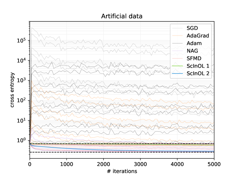
(a) Entire view of the results with logarithmic scale.

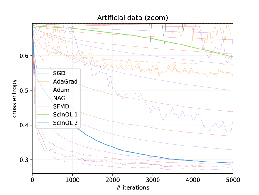
(b) Zoomed-in fragment showing best performers.

Figure 1: Average cross entropy from test set for the toy example.

To empirically demonstrate a need for scale invariance we tested our algorithms against some popular adaptive variants of OGD. The tests were run on a simple artificial binary classification dataset that mildly exaggerates relative magnitudes of features (however still keeps them in reasonable ranges). The dataset contains 21 real features, values of which are drawn from normal distributions $N(0,\sigma_{i})$, where $\sigma_{i}=2^{i-11}$ ($i=1,\ldots,21$), so that the scales of features vary from $2^{-10}$ to $2^{10}$ (the ratio of the largest and the smallest scale is of order $10^{6}$). Binary class labels where drawn from a Bernoulli distribution with $\Pr(y=1|\bm{x})=\mathrm{sigmoid}(\bm{x}^{\top}\bm{u})$ where $u_{i}=\pm\frac{1}{\sigma_{i}}$ with signs chosen uniformly at random. Note that $\bm{u}$ is set to compensate the scale of features and keep the predictions function $\bm{x}^{\top}\bm{u}$ to be of order of unity. We have drawn 5 000 training examples and 100 000 test examples. We repeated the experiment on 10 random training sets to decrease the variation of the results.

The algorithms were trained by minimizing the logistic loss (cross entropy loss) in an online fashion. Following similar experiments in the past papers concerning online methods (Kingma & Ba, 2014; Ross et al., 2013; Orabona & Tommasi, 2017), we report the average loss on the test set (after every 50 iterations) rather than the regret. We tested the following algorithms: OGD with learning rate decaying as $\eta_{t}=\eta/\sqrt{t}$ (called SGD here from stochastic gradient descent), AdaGrad (Duchi et al., 2011), Adam (Kingma & Ba, 2014), two scale-invariant algorithms from past work: NAG (Normalized Adaptive Gradient) (Ross et al., 2013) and Scale-free Mirror Descent by Orabona et al. (2015) (SFMD), and algorithms from this work. All algorithms except ours have a learning rate parameter, which in each case was set to values from $\{0.001,0.005,0.01,0.05,0.1,0.5,1,5,10\}$ (results concerning all learning rates were reported). We implemented our algorithms in Tensorflow and used existing implementations whenever it was possible.

Figure 1 shows average cross entropy measured on test set as a function of the number of iterations. Lines of the same color show results for the same algorithm but with different learning rates. Figure 1(a) uses logarithmic scale for $y$ axis: note the extreme values of the loss for most of the non-invariant algorithms. In fact, the two black dashed lines mark the loss achieved by the best possible model $\bm{u}$ (lower line) and a model with zero weight vector (upper line), so that every method above the upper dashed line does something worse than such a trivial baseline. Figure 1(b) shows only the fragment between dashed lines using linear scale for $y$ axis.

The results clearly show that algorithms which are not invariant to feature scales (SGD, Adam, and AdaGrad) are unable to achieve any reasonable result for any choice of the learning rate (most of the time performing much worse than the zero vector). This is because a single learning rate is unable to compensate all feature scales at the same time. The scale invariant algorithms, NAG and SFMD, perform much better (achieving the best overall results), but their behavior still depends on the learning rate tuning. Among our algorithms, ScInOL₁ slowly decreases its loss moving away from the initial zero solution, but it is clearly too slow in this problem. On the other hand, ScInOL₂ was able to achieve descent results without any tuning at all.

4.2 Linear Classification

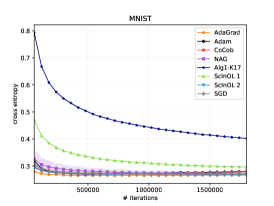
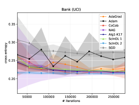
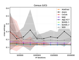
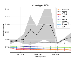
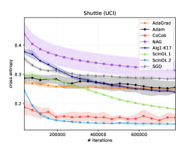
Figure 2: Mean test set cross entropy loss. Average values from 10 runs are depicted, shadows show $\pm$ standard deviation.

To further check empirical performance of our algorithms we tested them on some popular real-life benchmark datasets. We chose 5 datasets with varying levels of feature scale variance from UCI repository (Dheeru & Karra Taniskidou, 2017) (Covertype, Census, Shuttle, Bank, Madelon) and a popular benchmark dataset MNIST (LeCun & Cortes, 2010). For all datasets, categorical features were one-hot-encoded into multiple features and missing values were replaced by dedicated substitute features. Datasets that do not provide separate testing sets were split randomly into training/test sets ($2/1$ ratio). Short summary of datasets can be found in Appendix E.

Algorithms were trained by minimizing the cross entropy loss in an online fashion. Some of the data sets concern multiclass classification, which is beyond the framework considered here, as it would require multivariate prediction $\widehat{\bm{y}}=(\widehat{y}_{1},\ldots,\widehat{y}_{K})$ for each of $K$ classes, but it is straightforward to extend our setup to such multivariate case (details are given in Appendix G). To gain more insight into the long-term behavior of the algorithms, we trained all algorithms for multiple epochs. Each epoch consisted of running through the entire training set (shuffled) and testing average cross entropy and accuracy on the test set. Each algorithm was run 10 times for stability. We compared our algorithms with the following methods: SGD (with $\eta_{t}\sim 1/\sqrt{t}$), AdaGrad, Adam, NAG, CoCoB (Orabona & Tommasi, 2017) (an adaptive parameter-free algorithm; we used its Tensorflow implementation), and Algorithm 1 (coordinate-wise scale invariant method) by Kotłowski (2017) (which we call Alg1-K17). The algorithms using hand-picked learning rates (SGD, AdaGrad, Adam, NAG) were run with values from $\{0.00001,0.0001,0.001,0.01,0.1,1.0\}$ (all other parameters were kept default), and only the best test set results were reported (note that this biases the results in favour of these algorithms).

Figure 2 shows mean (test set) cross entropy loss (classification accuracy, given in Appendix F, leads to essentially the same conclusions); shaded areas around each curve depicts $\pm$ one standard deviation (over different runs). All graphs start with the error measured after the first epoch for better readability. The most noticeable fact in the plots is comparatively high variance (between different runs) of SGD, AdaGrad, Adam and NAG, i.e. the approaches with tunable learning rate. They also often performed worse than the remaining algorithms. Among our methods, ScInOL₂ turned out to perform better than ScInOL₁ in every case, due to its more aggressive updates. Note, however, that both algorithms are surprisingly stable, exhibiting very small variance in their performance across different runs. The best performance was most of the time achieved by either ScInOL₂ or CoCoB. Alg1-K17 was often converging somewhat slower (which is most pronounced for MNIST data), which we believe is due to its very conservative update policy.

5 Conclusions and future work

We proposed two online algorithms which behavior is invariant under arbitrary rescaling of individual features. The algorithms do not require any prior knowledge on the scale of the instances or the comparator and achieve, without any parameter tuning, regret bounds which match (up to a logarithmic factor) the regret bound of Online Gradient Descent with optimally tuned separate learning rates per dimension. The algorithms run in $O(d)$ per trial, which is comparable to the runtime of vanilla OGD.

The framework considered in this paper concerns well-understood and relatively simple linear models with convex objectives. It would be interesting to evaluate the importance of scale-invariance for deep learning methods, comprised of multiple layers connected by non-linear activation functions. As scale-invariance leads to well-conditioned algorithms, we believe that it could not only avoid the need for prior normalization of the inputs to the network, but it would also make the algorithm be independent of the scale of the inputs fed forward to the next layers. A scale-invariant update for neural nets might be robust against the “internal covariance shift” phenomenon (Ioffe & Szegedy, 2015) and avoid the need for batch normalization.

Finally, the potential functions we use to analyze our updates seems closely related to the potential function of EGU^± (Kivinen & Warmuth, 1997). It may be that our tuned online updates are simply approximation of (a version of) EGU^± and this needs further investigation.

Appendix A Bound for Online Gradient Descent with per-dimension learning rates

We remind the update of OGD with per-dimension learning rates:

$$w_{t+1,i}=w_{t,i}-\eta_{i}\nabla_{t,i},\qquad i=1,\ldots,d,$$

with $\bm{w}_{1}=\bm{0}$. For any $u_{i}\in\mathbb{R}$, we have:

$$(u_{i}-w_{t+1,i})^{2}-(u_{i}-w_{t,i})^{2}=(u_{i}-w_{t,i}+\eta_{i}\nabla_{t,i})^{2}-(u_{i}-w_{t,i})^{2}=2\eta_{i}\nabla_{t,i}(u_{i}-w_{t,i})+\eta_{i}^{2}\nabla_{t,i}^{2}.$$

Summing over trials $t=1,\ldots,T$ and rearranging:

$$2\eta_{i}\sum_{t=1}^{T}\nabla_{t,i}(w_{t,i}-u_{i})=u_{i}^{2}-(u_{i}-w_{T+1,i})^{2}+\eta_{i}^{2}\sum_{t=1}^{T}\nabla_{t,i}^{2}.$$

Dividing by $2\eta_{i}$, upper bounding and summing over $i=1,\ldots,d$:

$$\sum_{t=1}^{T}\nabla_{t}^{\top}(\bm{w}_{t}-\bm{u})\leq\sum_{i=1}^{d}\left(\frac{u_{i}^{2}}{2\eta_{i}}+\frac{\eta_{i}}{2}\sum_{t=1}^{T}\nabla_{t,i}^{2}\right).$$

Finally, using (3) shows that the right-hand side of the above upper bounds the regret.

Appendix B Scale invariance of Algorithm 1 and Algorithm 2

Let $\{(\bm{x}_{t},y_{t})\}_{t=1}^{T}$ be a data sequence and define a transformed sequence $\{(\bm{A}\bm{x}_{t},y_{t})\}_{t=1}^{T}$, where $\bm{A}=\mathrm{diag}(a_{1},\ldots,a_{d})$ with $a_{1},\ldots,a_{d}>0$. We will show that the sequence of predictions $\widehat{y}_{1},\ldots,\widehat{y}_{T}$ generated by the algorithms on the original and the transformed data sequences are the same. This can easily be done inductively: assuming $\widehat{y}_{1},\ldots,\widehat{y}_{t}$ are the same on both sequences, this implies $g_{1},\ldots,g_{t}$ are also the same (as $g_{t}=\partial_{\widehat{y}_{t}}\ell(y_{t},\widehat{y}_{t})$, while $y_{t}$ are the same in both sequences). Given that, a closer inspection of the algorithms lets us determine the behavior of all maintained statistics under the feature transformation $x_{t,i}\mapsto a_{i}x_{t,i}$.

For both algorithms we have:

$$M_{t,i}=\max_{j\leq t}|x_{j,i}|\mapsto a_{i}M_{t,i},\quad S_{t,i}^{2}=\sum_{j\leq t}(g_{j}x_{j,i})^{2}\mapsto a_{i}^{2}S_{t,i}^{2},\quad G_{t,i}=-\sum_{j\leq t}g_{j}x_{j,i}\mapsto a_{i}G_{t,i},$$

This means that for Algorithm 1:

$$\beta_{t,i}\mapsto\beta_{t,i},\quad\theta_{t,i}\mapsto\theta_{t,i},\quad w_{t,i}\mapsto a_{i}^{-1}w_{t,i},$$

so that $x_{t,i}w_{t,i}\mapsto x_{t,i}w_{t,i}$ and thus $\widehat{y}_{t}=\bm{x}_{t}^{\top}\bm{w}_{t}$ is invariant under the scale transformation.

Similarly, for Algorithm 2 we have:

$$\eta_{t,i}\mapsto\eta_{t,i},\quad\theta_{i,i}\mapsto\theta_{t,i},\quad w_{t,i}\mapsto a_{i}^{-1}w_{t,i},$$

and the scale invariance follows.

Appendix C Proof of Theorem 3.1

Before proving the theorem, we need two auxiliary results:

Lemma C.1.

Let $f(x)=\alpha\left(e^{|x|/\gamma}-|x|/\gamma-1\right)$ with $\alpha,\gamma>0$. Its Fenchel conjugate is given by:

$$\begin{split}f^{*}(u)\leavevmode\nobreak\ \stackrel{{\scriptstyle def}}{{=}}&\leavevmode\nobreak\ \sup_{x}\{ux-f(x)\}\\ \leavevmode\nobreak\ =\leavevmode\nobreak\ &(|u|\gamma+\alpha)\ln(1+|u|\gamma/\alpha)-|u|\gamma\\ \leavevmode\nobreak\ \leq\leavevmode\nobreak\ &|u|\gamma\ln(1+|u|\gamma/\alpha).\end{split}$$ (6)

Proof.

Note that since $f(x)$ is symmetric in $x$,

$$\begin{split}\sup_{x}\{ux-f(x)\}&=\sup_{x\geq 0}\{|u|x-f(x)\}\\ &=\sup_{x\geq 0}\Big{\{}\underbrace{|u|x-\alpha\left(e^{x/\gamma}-x/\gamma-1\right)}_{g(x)}\Big{\}}.\end{split}$$ (7)

Setting the derivative of $g(x)$ to zero gives its unconstrained maximizer $x^{*}=\gamma\ln(1+|u|\gamma/\alpha)$, and since $x^{*}\geq 0$, it is also the maximizer of $g(x)$ under constraint $x\geq 0$. Thus:

$$f^{*}(u)=g(x^{*})=(|u|\gamma+\alpha)\gamma\ln(1+|u|\gamma/\alpha)-|u|\gamma.$$

The inequality in the lemma follows from an elementary inequality $\ln(1+x)\leq x$ applied to $\alpha\ln(1+|u|\gamma/\alpha)$. ∎

Lemma C.2.

For any $v\in\mathbb{R}$ and any $q\in[-1,1]$:

$$\frac{q\;\mathrm{sgn}(v)}{2}\left(e^{\frac{|v|}{2}}-1\right)+e^{\frac{|v-q|}{2\sqrt{1+q^{2}}}}-\frac{|v-q|}{2\sqrt{1+q^{2}}}\leq e^{\frac{|v|}{2}}-\frac{|v|}{2}+q^{2}.$$

Proof.

It suffices to prove the lemma for $v\geq 0$. Indeed, the inequality holds for some $v\geq 0$ and $q\in[-1,1]$ if and only if it holds for $-v$ and $-q$. Denote:

$$\widetilde{v}=\frac{|v-q|}{\sqrt{1+q^{2}}}.$$

In this notation and with the assumption $v\geq 0$, the inequality translates to:

$$e^{\frac{\widetilde{v}}{2}}-\frac{\widetilde{v}}{2}\leq e^{\frac{v}{2}}\left(1-\frac{q}{2}\right)-\frac{v-q}{2}+q^{2}$$ (8)

We will split the proof into three sub-cases: (i) $q\geq v$, (ii) $q\leq v\leq 3$, and (iii) $v\geq 3$. Since $q\leq 1$, these cases cover all allowed values of $v$ and $q$.

Case (i): $q\geq v$.

We have $\widetilde{v}=\frac{q-v}{\sqrt{1+q^{2}}}\leq q-v$. Since the function $e^{x}-x$ is increasing in $x$ for $x\in(1,\infty)$, it holds:

$$e^{\frac{\widetilde{v}}{2}}-\frac{\widetilde{v}}{2}\leq e^{\frac{q-v}{2}}-\frac{q-v}{2}=e^{\frac{v}{2}}e^{\frac{q-2v}{2}}-\frac{q-v}{2}.$$

From $q\leq 1$ and $v\geq 0$ it follows $\frac{q-2v}{2}\leq\frac{1-2v}{2}\leq\frac{1}{2}$. Since function $f(x)=\frac{e^{x}-x-1}{x^{2}}$ is nondecreasing in $x$ (see, e.g., (Cesa-Bianchi & Lugosi, 2006), Section A.1.2), we have:

$$e^{x}-x-1\leq x^{2}\frac{e^{1/2}-1/2-1}{1/4}\leq 0.6x^{2}\qquad\text{for\leavevmode\nobreak\ \leavevmode\nobreak\ }x\leq\frac{1}{2}.$$ (9)

Thus, we bound $e^{\frac{q-2v}{2}}$ by $1+\frac{q-2v}{2}+0.15(q-2v)^{2}$ and get:

$$e^{\frac{\widetilde{v}}{2}}-\frac{\widetilde{v}}{2} \leq e^{\frac{v}{2}}\left(1+\frac{q-2v}{2}\right)-\frac{q-v}{2}+0.15e^{\frac{v}{2}}(q-2v)^{2}$$

$$=e^{\frac{v}{2}}\left(1-\frac{q}{2}\right)-\frac{v-q}{2}+(e^{\frac{v}{2}}-1)(q-v)+0.15e^{\frac{v}{2}}(q-2v)^{2}$$

$$\leq e^{\frac{v}{2}}\left(1-\frac{q}{2}\right)-\frac{v-q}{2}+v(q-v)+\frac{1}{4}(q-2v)^{2},$$

where the last inequality follows from the fact that $v\leq 1$ (as $q\geq v$ and $q\leq 1$), which by (9) implies $e^{\frac{v}{2}}\leq 1+\frac{v}{2}+0.6\frac{v^{2}}{4}=1+0.5v+0.15v^{2}\leq 1+v$, and furthermore $0.15e^{\frac{v}{2}}\leq 0.15e^{\frac{1}{2}}\leq\frac{1}{4}$. But $v(q-v)+\frac{1}{4}(q-2v)^{2}=\frac{1}{4}q^{2}\leq q^{2}$, which proves (8) for $q\geq v$.

Case (ii): $q\leq v\leq 3$.

We have $\widetilde{v}=\frac{v-q}{\sqrt{1+q^{2}}}\leq v-q$, and by the monotonicity of function $e^{x}-x$ for $x\in(1,\infty)$:

$$e^{\frac{\widetilde{v}}{2}}-\frac{\widetilde{v}}{2}\leq e^{\frac{v-q}{2}}-\frac{v-q}{2}=e^{\frac{v}{2}}e^{-\frac{q}{2}}-\frac{v-q}{2}.$$

Using (9) and $q\geq-1$, we bound $e^{-q/2}\leq 1-\frac{q}{2}+0.15q^{2}$ to get:

$$e^{\frac{\widetilde{v}}{2}}-\frac{\widetilde{v}}{2}\leq e^{\frac{v}{2}}\left(1-\frac{q}{2}\right)-\frac{v-q}{2}+0.15e^{\frac{v}{2}}q^{2}.$$

Using $0.15e^{\frac{v}{2}}\leq 0.15e^{\frac{3}{2}}\leq 0.68\leq 1$ proves (8) for $q\leq v\leq 3$.

Case (iii): $v>3$.

We lower-bound the right-hand side of (8):

$$e^{\frac{v}{2}}\left(1-\frac{q}{2}\right)-\frac{v-q}{2}+q^{2}\geq e^{\frac{v}{2}}\left(1-\frac{q}{2}\right)-\frac{v-q-\frac{q^{2}}{2}}{2}\geq e^{\frac{1}{2}(v-q-\frac{q^{2}}{2})}-\frac{v-q-\frac{q^{2}}{2}}{2},$$

where the first inequality is simply from $q^{2}\geq\frac{q^{2}}{4}$, while the second follows from $1-x\geq e^{-x-x^{2}}$ for $x\leq\frac{1}{2}$ (see, .e.g., (Cesa-Bianchi & Lugosi, 2006), Lemma 2.4). Now, using the monotonicity of function $e^{x}-x$,

$$e^{\frac{1}{2}(v-q-\frac{q^{2}}{2})}-\frac{v-q-\frac{q^{2}}{2}}{2}\geq e^{\frac{\widetilde{v}}{2}}-\frac{\widetilde{v}}{2}\qquad\iff\qquad v-q-\frac{q^{2}}{2}\geq\widetilde{v},$$

thus it suffices to show the latter to finish the proof. We have:

$$v-q-\frac{q^{2}}{2}-\widetilde{v}=(v-q)\left(1-\frac{1}{\sqrt{1+q^{2}}}\right)-\frac{q^{2}}{2}\geq(3-q)\left(1-\frac{1}{\sqrt{1+q^{2}}}\right)-\frac{q^{2}}{2}.$$

Using elementary inequality $\sqrt{1+x}\leq 1+\frac{x}{2}$, we have: $\frac{1}{\sqrt{1+q^{2}}}=\frac{\sqrt{1+q^{2}}}{1+q^{2}}\leq\frac{1+q^{2}/2}{1+q^{2}}$, and thus:

$$v-q-\frac{q^{2}}{2}-\widetilde{v} \geq(3-q)\left(1-\frac{1+q^{2}/2}{1+q^{2}}\right)-\frac{q^{2}}{2}=(3-q)\frac{q^{2}/2}{1+q^{2}}-\frac{q^{2}}{2}$$

$$=\frac{q^{2}}{2}\left(\frac{3-q}{1+q^{2}}-1\right)\geq\frac{q^{2}}{2}\left(\frac{3-1}{1+1}-1\right)=0.$$

This shows that $v-q-\frac{q^{2}}{2}\geq\widetilde{v}$ and thus proves (9) for $v>3$. ∎

Before we state the next result, we summarize the notation which will be used in what follows. For any $i=1,\ldots,d$ and any $t=1,\ldots,T$, let:

$$M_{t,i}=\max_{j\leq t}|x_{j,i}|,\qquad G_{t,i}=-\sum_{j\leq t}g_{j}x_{j,i},\qquad S^{2}_{t,i}=\sum_{j\leq t}(g_{j}x_{j,i})^{2},$$

be, respectively, the maximum input value, the negative cumulative gradient, and the sum of squared gradients at $i$-th coordinate up to (and including) trial $t$, and we also denote $M_{0,i}=G_{0,i}=S^{2}_{0,i}=0$. Moreover, define:

$$\beta_{t,i}=\left\{\begin{array}[]{ll}\min\left\{\beta_{t-1,i},\epsilon\frac{S_{t-1,i}^{2}+M_{t,i}^{2}}{x_{t,i}^{2}t}\right\}&\quad\text{when\leavevmode\nobreak\ \leavevmode\nobreak\ }x_{t,i}\neq 0,\\ \beta_{t-1,i}&\quad\text{when\leavevmode\nobreak\ \leavevmode\nobreak\ }x_{t,i}=0,\end{array}\right.$$

with $\beta_{1,i}=\epsilon$. The weight vector at trial $t$ is given by:

$$w_{t,i}=\frac{\beta_{t,i}\mathrm{sgn}(G_{t-1,i})}{2\sqrt{S_{t-1,i}^{2}+M_{t,i}^{2}}}\left(e^{\frac{|G_{t-1,i}|}{2\sqrt{S_{t-1,i}^{2}+M_{t,i}^{2}}}}-1\right),$$ (10)

as long as $M_{t,i}>0$; if $M_{t,i}=0$ (which means that $x_{j,i}=0$ for all $j\leq t$), we set $w_{t,i}=0$, but any other value of $w_{t,i}$ would lead to the same loss. Finally, define $\hat{S}^{2}_{t,i}=S^{2}_{t,i}+M^{2}_{t,i}$.

Lemma C.3.

Define:

$$\psi_{t,i}(x)=\left\{\begin{array}[]{ll}\beta_{t,i}\left(e^{|x|/(2\hat{S}_{t,i})}-\frac{|x|}{2\hat{S}_{t,i}}-1\right)&\quad\text{for\leavevmode\nobreak\ \leavevmode\nobreak\ }\hat{S}_{t,i}\neq 0,\\ 0&\quad\text{for\leavevmode\nobreak\ \leavevmode\nobreak\ }\hat{S}_{t,i}=0.\end{array}\right.$$

For any $i=1,\ldots,d$ and any $t=1,\ldots,T$ we have:

$$w_{t,i}g_{t}x_{t,i}\leavevmode\nobreak\ \leq\leavevmode\nobreak\ \psi_{t-1,i}(G_{t-1,i})-\psi_{t,i}(G_{t,i})+\frac{\epsilon}{t}.$$

Proof.

Fix $i\in\{1,\ldots,d\}$, and let $\tau_{i}$ be the first trial $t$ such that $x_{t,i}\neq 0$. This means that $\hat{S}_{t,i}=x_{t,i}=0$ for all $t<\tau_{i}$, and the inequality is trivially satisfied for any $t<\tau_{i}$, as the left-hand side is zero, while the right-hand side is $\epsilon/t$. Thus, assume $t\geq\tau_{i}$.

Fix $t$ and define $v=\frac{G_{t-1,i}}{\sqrt{S_{t-1,i}^{2}+M_{t,i}^{2}}}$ and $q=\frac{g_{t}x_{t,i}}{\sqrt{S_{t-1,i}^{2}+M_{t,i}^{2}}}$. As $|q|\leq\frac{|g_{t}x_{t,i}|}{M_{t,i}}\leq\frac{|x_{t,i}|}{\max_{j\leq t}|x_{j,i}|}\leq 1$, we can apply Lemma C.2 to such $v$ and $q$, which, after subtracting $1$ and multiplying by $\beta_{t,i}$ on both sides, gives:

$$\beta_{t,i}\frac{q\;\mathrm{sgn}(v)}{2}\left(e^{\frac{|v|}{2}}-1\right) +\beta_{t,i}\left(e^{\frac{|v-q|}{2\sqrt{1+q^{2}}}}-\frac{|v-q|}{2\sqrt{1+q^{2}}}-1\right)$$

$$\leq\beta_{t,i}\left(e^{\frac{|v|}{2}}-\frac{|v|}{2}-1\right)+\beta_{t,i}q^{2}.$$ (11)

Using the definition of the weight vector (10) we identify the first term on the left-hand side of (11):

$$\beta_{t,i}\frac{q\;\mathrm{sgn}(v)}{2}\left(e^{|v|/2}-1\right)=w_{t,i}g_{t}x_{t,i}.$$

Next, since:

$$\frac{G_{t,i}}{\hat{S}_{t,i}}=\frac{G_{t,i}}{\sqrt{S_{t,i}^{2}+M_{t,i}^{2}}}=\frac{G_{t-1,i}-g_{t}x_{t,i}}{\sqrt{S_{t-1,i}^{2}+M_{t,i}^{2}+(g_{t}x_{t,i})^{2}}}=\frac{v-q}{\sqrt{1+q^{2}}},$$

the second term on the left-hand side of (11) is equal to $\psi_{t,i}(G_{t,i})$. Thus, (11) can be rewritten as:

$$w_{t,i}g_{t}x_{t,i}+\psi_{t,i}(G_{t,i})\leq\beta_{t,i}\left(e^{\frac{|v|}{2}}-\frac{|v|}{2}-1\right)+\beta_{t,i}q^{2},$$

and to finish the proof, it suffices to show that the two terms on the right-hand side are upper bounded, respectively, by $\psi_{t-1,i}(G_{t-1,i})$ and $\frac{\epsilon}{t}$.

To bound $\beta_{t,i}q^{2}$ note that if $x_{t,i}=0$ then $\beta_{t,i}q^{2}=0$, whereas if $x_{t,i}\neq 0$ then by the definition of $\beta_{t,i}$:

$$\beta_{t,i}q^{2}=\beta_{t,i}\frac{(g_{t}x_{t,i})^{2}}{S_{t-1,i}^{2}+M_{t,i}^{2}}\leq\epsilon\frac{S_{t-1,i}^{2}+M_{t,i}^{2}}{x_{t,i}^{2}t}\frac{(g_{t}x_{t,i})^{2}}{S_{t-1,i}^{2}+M_{t,i}^{2}}\leq\frac{\epsilon g_{t}^{2}}{t}\leq\frac{\epsilon}{t}.$$

To bound $\beta_{t,i}(e^{|v|/2}-|v|/2-1)$ by $\psi_{\tau_{i}-1,i}(G_{t-1,i})$ note that both are zero if $t=\tau_{i}$ (because $G_{\tau_{i}-1,i}=0$ and $v=0$). On the other hand, for $t>\tau_{i}$ we have:

$$|v|=\frac{|G_{t-1,i}|}{\sqrt{S_{t-1,i}^{2}+M_{t,i}^{2}}}\leq\frac{|G_{t-1,i}|}{\sqrt{S_{t-1,i}^{2}+M_{t-1,i}^{2}}}=\frac{|G_{t-1,i}|}{\hat{S}_{t-1,i}},$$

and by the monotonicity of $f(x)=e^{x}-x-1$:

$$\beta_{t,i}(e^{|v|/2}-|v|/2-1)\leq\beta_{t,i}\left(e^{\frac{|G_{t-1,i}|}{2\hat{S}_{t-1,i}}}-\frac{|G_{t-1,i}|}{2\hat{S}_{t-1,i}}-1\right)\leq\psi_{t-1,i}(G_{t-1,i}),$$

where in the last inequality we used $\beta_{t,i}\leq\beta_{t-1,i}$ (which follows from the definition) and the fact that $e^{x}-x-1\geq 0$ for all $x$. ∎

We are now ready to prove Theorem 3.1, which we restate here for convenience:

Theorem.

For any $\bm{u}\in\mathbb{R}$ the regret of $\mathrm{ScInOL}_{1}$ is upper-bounded by:

$$R_{T}(\bm{u})\leq\sum_{i=1}^{d}\left(2|u_{i}|\hat{S}_{T,i}\ln(1+2|u_{i}|\hat{S}_{T,i}\epsilon^{-1}T)+\epsilon(1+\ln T)\right)=\sum_{i=1}^{d}\tilde{O}(|u_{i}|\hat{S}_{T,i}),$$

where $\hat{S}_{T,i}=\sqrt{S_{T,i}^{2}+M_{T,i}^{2}}$ and $\tilde{O}(\cdot)$ hides the constants and logarithmic factors.

Proof.

Applying Lemma (C.3) for a fixed $i\in\{1,\ldots,d\}$ and all $t=1,\ldots,T$, and summing over trials gives:

$$\sum_{t=1}^{T}w_{t,i}g_{t}x_{t,i}\leq-\psi_{T,i}(G_{T,i})+\sum_{t=1}^{T}\frac{\epsilon}{t}\leq-\psi_{T,i}(G_{T,i})+\epsilon\left(1+\ln T\right),$$

where we used $\psi_{0,i}(G_{0,i})=0$. By (3),

$$R_{T}(\bm{u}) \leq\sum_{t=1}^{T}g_{t}\bm{x}_{t}^{\top}(\bm{w}_{t}-\bm{u})=\sum_{i=1}^{d}\left(\sum_{t=1}^{T}g_{t}x_{t,i}w_{t,i}+G_{T,i}u_{i}\right)$$

$$\leq\sum_{i=1}^{d}\left(G_{T,i}u_{i}-\psi_{T,i}(G_{T,i})\right)+d\epsilon\left(1+\ln(T)\right)$$

$$\leq\sum_{i=1}^{d}\sup_{x}\left\{xu_{i}-\psi_{T,i}(x)\right\}+d\epsilon\left(1+\ln(T)\right)$$

$$\leq\sum_{i=1}^{d}2|u_{i}|\hat{S}_{T,i}\ln\left(1+2|u_{i}|\hat{S}_{T,i}/\beta_{T,i}\right)+d\epsilon\left(1+\ln(T)\right),$$

where in the last inequality we used Lemma C.1 for each $i$ with $\alpha=\beta_{T,i}$ and $\gamma=2\hat{S}_{T,i}$. To finish the proof, it suffices to show that $\beta_{T,i}\geq\frac{\epsilon}{T}$, which we do by induction on $t$. For $t=1$, we have by the definition $\beta_{t,i}=\epsilon$. Now, assume $\beta_{t-1,i}\geq\frac{\epsilon}{t-1}$, and we will show $\beta_{t,i}\geq\frac{\epsilon}{t}$. If $x_{t,i}=0$, $\beta_{t,i}=\beta_{t-1,i}\geq\frac{\epsilon}{t-1}>\frac{\epsilon}{t}$; on the other hand, if $x_{t,i}\neq 0$, from the definition of $\beta_{t,i}$:

$$\beta_{t,i}=\min\left\{\beta_{t-1,i},\epsilon\frac{S_{t-1,i}^{2}+M_{t,i}^{2}}{x_{t,i}^{2}t}\right\}\geq\min\left\{\frac{\epsilon}{t-1},\epsilon\frac{x_{t,i}^{2}}{x_{t,i}^{2}t}\right\}=\frac{\epsilon}{t},$$

where we used $S_{t-1,i}^{2}+M_{t,i}^{2}\geq M_{t,i}^{2}=\max_{j\leq t}x_{j,i}^{2}\geq x_{t,i}^{2}$. ∎

Appendix D Proof of Theorem 3.2

Figure 3: Function $h(x)$

Similarly as in the previous section, we proceed the proof of the theorem with several auxiliary results. Define:

$$h(x)=\left\{\begin{array}[]{ll}\frac{1}{2}x^{2}&\qquad\text{for\leavevmode\nobreak\ }|x|\leq 1,\\ |x|-\frac{1}{2}&\qquad\text{for\leavevmode\nobreak\ }|x|>1\end{array}\right.$$ (12)

(see Figure 3). Note that $h(x)=h(|x|)$, and $h(|x|)$ is monotonic in $|x|$. Moreover, for all $x\in\mathbb{R}$:

$$|x|-\frac{1}{2}\leq h(x)\leq\frac{1}{2}x^{2}.$$ (13)

The lower bound in (13) is clearly satisfied for $|x|<1$, while for $|x|\leq 1$ we have $h(x)-(|x|-\frac{1}{2})=\frac{1}{2}(|x|-1)^{2}\geq 0$. On the other hand, the upper bound in (13) is clearly satisfied for $|x|\leq 1$, while for $|x|>1$ we have $h(x)-\frac{1}{2}x^{2}=-\frac{1}{2}(|x|-1)^{2}\leq 0$.

Lemma D.1.

Let $f(x)=\alpha e^{|x|/\gamma}$ with $\alpha,\gamma>0$. Its Fenchel conjugate $f^{*}(u)=\sup_{x}\{ux-f(x)\}$ satisfies $f^{*}(u)\leq|u|\gamma(\ln(|u|\gamma/\alpha)-1)$ for all $u$.

Proof.

Since $f(x)$ is symmetric in $x$, $\sup_{x}\{ux-f(x)\}=\sup_{x\geq 0}\{|u|x-f(x)\}=\sup_{x\geq 0}g(x)$, where $g(x)=|u|x-\alpha e^{x/\gamma}$. Setting the derivative of $g(x)$ to zero gives its unconstrained maximizer $x^{*}=\gamma\ln(|u|\gamma/\alpha)$, for which $g(x^{*})=|u|\gamma(\ln(|u|\gamma/\alpha)-1)$. The proof is finished by noticing that $\sup_{x\geq 0}g(x)\leq\sup_{x\in\mathbb{R}}g(x)=g(x^{*})$. ∎

Lemma D.2.

For any $v\in\mathbb{R}$ and any $q\in[-1,1]$:

$$\exp\left\{\frac{1}{2}h\left(\frac{v-q}{1+q^{2}}\right)-\frac{1}{2}h(v)-\frac{1}{2}q^{2}\right\}\leq 1-\frac{1}{2}q\;\mathrm{sgn}(v)\min\{|v|,1\}$$

Proof.

It suffices to prove the lemma for $v\geq 0$. Indeed, the inequality holds for some $v\geq 0$ and $q\in[-1,1]$ if and only if it holds for $-v$ and $-q$. Denote:

$$\widetilde{v}=\frac{|v-q|}{\sqrt{1+q^{2}}}.$$

In this notation and with the assumption $v\geq 0$, the inequality translates to:

$$e^{\frac{1}{2}(h(\widetilde{v})-h(v)-q^{2})}\leq 1-\frac{1}{2}q\min\{v,1\}.$$ (14)

To prove (14), it suffices to show that:

$$h(\widetilde{v})-h(v)-q^{2}\leq-q\min\{v,1\}-\frac{1}{2}(q\min\{v,1\})^{2},$$ (15)

because (15) together with $q\leq 1$ and inequality $e^{-x-x^{2}}\leq 1-x$ for $x\leq\frac{1}{2}$ (see, e.g., (Cesa-Bianchi & Lugosi, 2006), Section A.1.2) implies (14).

We will split the proof of (15) into three sub-cases: (i) $v\leq 1$, (ii) $v\geq 1$ and $\widetilde{v}\geq 1$, (iii) $v\geq 1$ and $\widetilde{v}<1$.

Case (i): $v\leq 1$.

From the definition, $h(v)=\frac{1}{2}v^{2}$ and by (13) we upper bound $h(\widetilde{v})\leq\frac{1}{2}\widetilde{v}^{2}$. Using $\widetilde{v}\leq|v-q|$ we have:

$$h(\widetilde{v})-h(v)-q^{2}\leq\frac{1}{2}\widetilde{v}^{2}-\frac{1}{2}v^{2}-q^{2}\leq\frac{1}{2}(v-q)^{2}-\frac{1}{2}v^{2}-q^{2}=-vq-\frac{1}{2}q^{2}\leq-vq-\frac{1}{2}v^{2}q^{2},$$

and since $\min\{v,1\}=v$, this implies (15).

Case (ii): $v\geq 1$ and $\widetilde{v}\geq 1$.

As $q\leq 1\leq v$, we have $|v-q|=v-q$, and by the definition, $h(v)=v-\frac{1}{2}$, $h(\widetilde{v})=\widetilde{v}-\frac{1}{2}$. Therefore:

$$h(\widetilde{v})-h(v)-q^{2}=\widetilde{v}-v-q^{2}\leq v-q-v-q^{2}\leq-q-q^{2}/2,$$

where in the first inequality we used $\widetilde{v}\leq|v-q|=v-q$. As $\min\{v,1\}=1$, this implies (15).

Case (iii): $v\geq 1$ and $\widetilde{v}<1$.

We have:

$$\widetilde{v}<1\;\iff\;\frac{(v-q)^{2}}{1+q^{2}}\leq 1\;\iff\;v^{2}-2vq-1\leq 0\;\iff\;v\leq q+\sqrt{1+q^{2}},$$

where the last equivalence follows from solving a quadratic inequality with respect to $v\geq 1$ for fixed $q$. We now note that function:

$$g(v)=h(\widetilde{v})-h(v)-q^{2}=\frac{1}{2}\widetilde{v}^{2}-\Big{(}v-\frac{1}{2}\Big{)}-q^{2}=\frac{(v-q)^{2}}{2(1+q^{2})}-v-q^{2}+\frac{1}{2}$$

is convex in $v$ and hence it is maximized at the boundaries $\{1,q+\sqrt{1+q^{2}}\}$ of the allowed range of $v$. When $v=1$, we have:

$$g(v)=\frac{(1-q)^{2}}{2(1+q^{2})}-1-q^{2}+\frac{1}{2}\leq\frac{1}{2}(1-q)^{2}-q^{2}-\frac{1}{2}=-q-\frac{1}{2}q^{2},$$

whereas if $v=q+\sqrt{1+q^{2}}$, we have

$$g(v)=\frac{1}{2}-\left(q+\sqrt{1+q^{2}}\right)-q^{2}+\frac{1}{2}\leq-q-q^{2}\leq-q-\frac{1}{2}q^{2},$$

so that $g(v)\leq-q-\frac{1}{2}q^{2}$ in the entire range of allowed values of $v$. As $\min\{v,1\}=1$, this implies (15). ∎

Before stating further results, we summarize the notation: for $i=1,\ldots,d$ and $t=1,\ldots,T$,

$$M_{t,i}=\max_{j\leq t}|x_{j,i}|,\quad G_{t,i}=-\sum_{j\leq t}g_{j}x_{j,i},\quad S^{2}_{t,i}=\sum_{j\leq t}(g_{j}x_{j,i})^{2},\quad\eta_{t,i}=\epsilon-\sum_{j\leq t}g_{t}x_{t,i}w_{t,i},$$

with the convention $M_{0,i}=G_{0,i}=S^{2}_{0,i}=0$ and $\eta_{0,i}=\epsilon$. As before, we also use $\hat{S}^{2}_{t,i}=S^{2}_{t,i}+M^{2}_{t,i}$. The weight vector at trial $t$ is given by:

$$w_{t,i}=\frac{\mathrm{sgn}(G_{t-1,i})\min\left\{\frac{|G_{t-1,i}|}{\sqrt{S_{t-1,i}^{2}+M_{t,i}^{2}}},1\right\}}{2\sqrt{S_{t-1,i}^{2}+M_{t,i}^{2}}}\eta_{t-1,i}$$ (16)

as long as $M_{t,i}>0$; if $M_{t,i}=0$, we set $w_{t,i}=0$.

Lemma D.3.

Define:

$$\psi_{t,i}(x)=\left\{\begin{array}[]{ll}e^{\frac{1}{2}h\big{(}\frac{x}{\hat{S}_{t,i}}\big{)}}&\quad\text{for\leavevmode\nobreak\ \leavevmode\nobreak\ }\hat{S}_{t,i}\neq 0,\\ 1&\quad\text{for\leavevmode\nobreak\ \leavevmode\nobreak\ }\hat{S}_{t,i}=0,\end{array}\right.$$

with $h(\cdot)$ defined in (12). For any $i=1,\ldots,d$, let $\tau_{i}$ be the first trial in which $x_{t,i}\neq 0$. We have for any $=1,\ldots,d$ and any $t=\tau_{i},\ldots,T$:

$$\frac{\eta_{t,i}}{\eta_{t-1,i}}\geq\frac{\psi_{t,i}(G_{t,i})}{\psi_{t-1,i}(G_{t-1,i})}e^{-\delta_{t,i}},$$

where $\delta_{t,i}=\frac{(g_{t}x_{t,i})^{2}}{2(S_{t-1,i}^{2}+M_{t,i}^{2})}$

Proof.

Fix $i$ and $t\geq\tau_{i}$, and define $v=\frac{G_{t-1,i}}{\sqrt{S_{t-1,i}^{2}+M_{t,i}^{2}}}$ and $q=\frac{g_{t}x_{t,i}}{\sqrt{S_{t-1,i}^{2}+M_{t,i}^{2}}}$. As $|q|\leq\frac{|g_{t}x_{t,i}|}{M_{t,i}}\leq 1$, we can apply Lemma D.2 to such $v$ and $q$, which gives:

$$e^{\frac{1}{2}h\left(\frac{v-q}{1+q^{2}}\right)-\frac{1}{2}h(v)-\frac{1}{2}q^{2}}\leq 1-\frac{1}{2}q\;\mathrm{sgn}(v)\min\{|v|,1\}$$ (17)

Using the definition of weight vector (16), we identify the right-hand side of (17) with $1-\frac{g_{t}x_{t,i}w_{t,i}}{\eta_{t-1,i}}=\frac{\eta_{t,i}}{\eta_{t-1,i}}$. Since $\frac{1}{2}q^{2}=\delta_{t,i}$ and $\frac{G_{t,i}}{\hat{S}_{t,i}}=\frac{v-q}{\sqrt{1+q^{2}}}$ (see the proof of Lemma C.3), we also identify the left-hand side of (17) with $\psi_{t,i}(G_{t,i})e^{-\frac{1}{2}h(v)}e^{-\delta_{t,i}}$. Hence, (17) can be rewritten as:

$$\frac{\eta_{t,i}}{\eta_{t-1,i}}\geq\frac{\psi_{t,i}(G_{t,i})}{e^{\frac{1}{2}h(v)}}e^{-\delta_{t,i}},$$

and thus to prove the lemma, it suffices to show:

$$e^{\frac{1}{2}h(v)}\leq\psi_{t-1,i}(G_{t-1,i}).$$ (18)

When $t=\tau_{i}$, we have $v=0$ as well as $G_{t-1,i}=0$, and (18) holds as its both sides are equal to $1$. For $t>\tau_{i}$, (18) reduces to $h(v)\leq h(G_{t-1,i}/\hat{S}_{t-1,i})$, which holds because:

$$|v|=\frac{|G_{t-1,i}|}{\sqrt{S_{t-1,i}^{2}+M_{t,i}^{2}}}\leq\frac{|G_{t-1,i}|}{\sqrt{S_{t-1,i}^{2}+M_{t-1,i}^{2}}}=\frac{|G_{t-1,i}|}{\hat{S}_{t-1,i}},$$

and $h(x)=h(|x|)$ is monotonic in $|x|$. ∎

We are now ready to prove Theorem 3.2, which we restate here for convenience:

Theorem.

For any $\bm{u}\in\mathbb{R}$ the regret of $\mathrm{ScInOL}_{2}$ is upper-bounded by:

$$R_{T}(\bm{u})\leq d\epsilon+\sum_{i=1}^{d}2|u_{i}|\hat{S}_{T,i}\left(\ln(3|u_{i}|\hat{S}^{3}_{T,i}\epsilon^{-1}/x_{\tau_{i},i}^{2})-1\right),$$

where $\hat{S}_{T,i}=\sqrt{S_{T,i}^{2}+M_{T,i}^{2}}$ and $\tau_{i}=\min\{t\colon|x_{t,i}|\neq 0\}$.

Proof.

Fixing $i\in\{1,\ldots,d\}$, applying Lemma (C.3) for $t=\tau_{i},\ldots,T$, and multiplying over trials gives:

$$\frac{\eta_{T,i}}{\eta_{\tau_{i}-1,i}}\geq\frac{\psi_{T,i}(G_{T,i})}{\psi_{\tau_{i}-1,i}(G_{\tau_{i}-1,i})}e^{-\Delta_{T,i}},$$

where we denoted $\Delta_{T,i}=\sum_{t=\tau_{i}}^{T}\delta_{t,i}$. From the definition of $\tau_{i}$, we have $\eta_{\tau_{i}-1,i}=\epsilon$ and $\psi_{\tau_{i}-1,i}\equiv 1$. Using $\eta_{T,i}=\epsilon-\sum_{t\leq T}g_{t}x_{t,i}w_{t,i}$ we get:

$$\sum_{t=1}^{T}g_{t}x_{t,i}w_{t,i}\leq\epsilon-\epsilon\psi_{T,i}(G_{T,i})e^{-\Delta_{T,i}}\leq\epsilon-\epsilon e^{-\Delta_{T,i}+|G_{T,i}|/(2\hat{S}_{T,i})-\frac{1}{4}},$$

where we used (12) to bound $h(x)\geq|x|-\frac{1}{2}$. By (3),

$$R_{T}(\bm{u}) \leq\sum_{t=1}^{T}g_{t}\bm{x}_{t}^{\top}(\bm{w}_{t}-\bm{u})=\sum_{i=1}^{d}\left(\sum_{t=1}^{T}g_{t}x_{t,i}w_{t,i}+G_{T,i}u_{i}\right)$$

$$\leq d\epsilon+\sum_{i=1}^{d}\left(G_{T,i}u_{i}-\epsilon e^{-\Delta_{T,i}-\frac{1}{4}}e^{|G_{T,i}|/(2\hat{S}_{T,i})}\right)$$

$$\leq d\epsilon+\sum_{i=1}^{d}\sup_{x}\left\{xu_{i}-\epsilon e^{-\Delta_{T,i}-\frac{1}{4}}e^{|x|/(2\hat{S}_{T,i})}\right\}$$

$$\leq d\epsilon+\sum_{i=1}^{d}2|u_{i}|\hat{S}_{T,i}\left(\ln\left(2\epsilon^{-1}|u_{i}|\hat{S}_{T,i}e^{\frac{1}{4}+\Delta_{T,i}}\right)-1\right),$$

where in the last inequality we used Lemma D.1 for each $i$ with $\alpha=\epsilon e^{-\Delta_{T,i}-\frac{1}{4}}$ and $\gamma=2\hat{S}_{T,i}$. We will now show that

$$\Delta_{T,i}\leq\ln\left(\frac{\hat{S}_{T,i}^{2}}{x_{\tau_{i},i}^{2}}\right),$$ (19)

which, together with $2e^{1/4}\leq 3$ will finish the proof. To prove (19), we use $M_{t,i}^{2}\geq x_{t,i}^{2}\geq(g_{t}x_{t,i})^{2}=S_{t,i}^{2}-S_{t-1,i}^{2}$ to get:

$$\delta_{t,i}=\frac{(g_{t}x_{t,i})^{2}}{2(S_{t-1,i}^{2}+M_{t,i}^{2})}\leq\frac{(g_{t}x_{t,i})^{2}}{S_{t-1,i}^{2}+2M_{t,i}^{2}}\leq\frac{(g_{t}x_{t,i})^{2}}{S_{t,i}^{2}+M_{t,i}^{2}}=\frac{(M_{t,i}^{2}+S_{t,i}^{2})-(M_{t,i}^{2}+S_{t-1,i}^{2})}{S_{t,i}^{2}+M_{t,i}^{2}}.$$

Using $\frac{a-b}{a}\leq\ln\frac{a}{b}$ for any $a\geq b>0$ (which follows from the concavity of the logarithm):

$$\delta_{t,i}\leq\ln\frac{M_{t,i}^{2}+S_{t,i}^{2}}{M_{t,i}^{2}+S_{t-1,i}^{2}}\leq\ln\frac{M_{t+1,i}^{2}+S_{t,i}^{2}}{M_{t,i}^{2}+S_{t-1,i}^{2}},$$

where for $t=T$, we define $M_{T+1,i}=M_{T,i}$. Summing the above over trials $t=\tau_{i},\ldots,T$:

$$\Delta_{T,i}=\sum_{t=\tau_{i}}^{T}\delta_{t,i}\leq\ln\frac{M_{T+1,i}^{2}+S_{T,i}^{2}}{M_{\tau_{i},i}^{2}+S_{\tau_{i}-1,i}^{2}}=\ln\frac{M_{T,i}^{2}+S_{T,i}^{2}}{x_{\tau_{i},i}^{2}}=\ln\frac{\hat{S}_{T,i}^{2}}{x_{\tau_{i},i}^{2}},$$

which was to be shown. ∎

Appendix E Datasets

MNIST dataset is available at Yann Lecun’s page. All other datasets are availableat the UCI repository. Scale is computed as a ratio of highest to lowest positive $L_{2}$ norms of features.

Name	features	records	classes	scale
Bank	53	41188	2	6.05E+05
Census	381	299285	2	1.81E+06
Covertype	54	581012	7	1.31E+06
Madelon	500	2600	2	1.09E+00
MNIST	728	70000	10	5.83E+03
Shuttle	9	58000	7	7.46E+00

Table 2: Short summary of datasets

Appendix F Experiment: classification accuracy plots

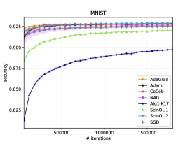
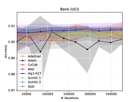
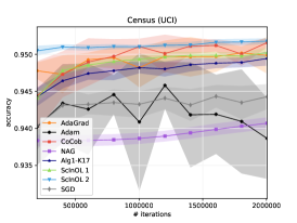
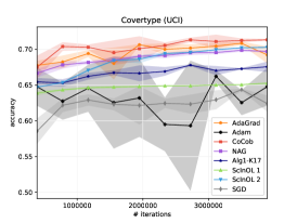
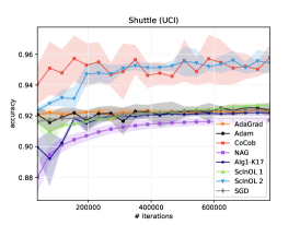
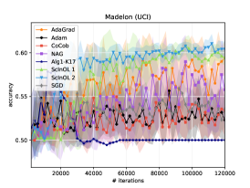
Figure 4: Accuracy results for linear classification experiments.

Appendix G Multivariate predictions

For simplicity, in the paper we focus on loss functions defined for real-valued predictions $\widehat{y}\in\mathbb{R}$. Sometimes, however, it is natural to consider a setup of multivariate predictions $\widehat{\bm{y}}\in\mathbb{R}^{K}$. For instance, the multinomial logistic loss (cross-entropy loss) is defined for $y\in\{1,\ldots,K\}$ as:

$$\ell(y,\widehat{\bm{y}})=-\sum_{k=1}^{K}\bm{1}[y=k]\ln\sigma_{k}(\widehat{\bm{y}})=-\widehat{y}_{y}+\ln\left(\sum_{k=1}^{K}e^{\widehat{y}_{k}}\right),$$

where $\sigma_{k}(\widehat{\bm{y}})=\frac{e^{\widehat{y}_{k}}}{\sum_{j=1}^{K}e^{\widehat{y}_{j}}}$ is the soft-max transform.

We assume the multivariate losses $\ell_{t}(\widehat{\bm{y}})=\ell(y_{t},\widehat{\bm{y}})$ are convex and $L$-Lipschitz in the sense that the max-norm of subgradient $\nabla\ell_{t}(\widehat{\bm{y}})$ for any $\widehat{\bm{y}}$ is bounded, $\|\nabla\ell_{t}(\widehat{\bm{y}})\|_{\infty}\leq L$ (which is satisfied with $L=1$ by the multinomial logistic loss). We consider the class of comparators which are parameterized by $\bm{U}\in\mathbb{R}^{d\times K}$, a $d\times K$ parameter matrix, and the regret of the algorithms against $\bm{U}$ for a sequence of data $\{(\bm{x}_{t},y_{t})\}_{t=1}^{T}$ is defined as:

$$R_{T}(\bm{U})=\sum_{t=1}^{T}\ell_{t}(\widehat{\bm{y}}_{t})-\sum_{t=1}^{T}\ell_{t}(\bm{U}^{\top}\bm{x}_{t}).$$

Consider an algorithm which at trial $t$ predicts with a weight matrix $\bm{W}_{t}\in\mathbb{R}^{d\times K}$, $\widehat{\bm{y}}_{t}=\bm{W}_{t}^{\top}\bm{x}_{t}$. Using the convexity of the loss, for any $\widehat{\bm{y}},\widehat{\bm{y}}^{\prime}$ and any $t$ we have $\ell_{t}(\widehat{\bm{y}}^{\prime})\geq\ell_{t}(\widehat{\bm{y}})+\nabla\ell_{t}(\widehat{\bm{y}})^{\top}(\widehat{\bm{y}}^{\prime}-\widehat{\bm{y}})$. Denoting $\nabla\ell_{t}(\widehat{\bm{y}}_{t})$ by $\bm{g}_{t}=(g_{t,1},\ldots,g_{t,K})$ with $g_{t,k}\in[-L,L]$ for all $k=1,\ldots,K$, and using the bound above with $\widehat{\bm{y}}=\widehat{\bm{y}}_{t}=\bm{W}_{t}^{\top}\bm{x}_{t}$ and $\widehat{\bm{y}}^{\prime}=\bm{U}^{\top}\bm{x}_{t}$ we have:

$$R_{T}(\bm{U})=\sum_{i=1}^{d}\sum_{k=1}^{K}\left(\sum_{t=1}^{T}g_{t,k}x_{t,i}(W_{t;i,k}-U_{i,k})\right).$$

The regret decouples into a sum over individual coordinates and dimensions of the prediction vector, and the extension of our algorithms is now straightforward (see Algorithm (3) and (4) below). Also, the analysis can be carried out in full analogy to the univariate loss case resulting in the following bounds (for $L=1$):

Theorem G.1.

For any $\bm{U}\in\mathbb{R}^{d\times K}$ the regret of $\mathrm{ScInOL}_{1}$ is upper-bounded by:

$$R_{T}(\bm{U})\leq\sum_{i=1}^{d}\sum_{k=1}^{K}\left(2|U_{i,k}|\hat{S}_{T;i,k}\ln(1+2|U_{i,k}|\hat{S}_{T;i,k}\epsilon^{-1}T)+\epsilon(1+\ln T)\right)$$

where $\hat{S}_{T;i,k}=\sqrt{S_{T;i,k}^{2}+M_{T;i}^{2}}$.

Theorem G.2.

For any $\bm{U}\in\mathbb{R}^{d\times K}$ the regret of $\mathrm{ScInOL}_{2}$ is upper-bounded by:

$$R_{T}(\bm{U})\leq dK\epsilon+\sum_{i=1}^{d}\sum_{k=1}^{K}2|U_{i,k}|\hat{S}_{T;i,k}\left(\ln(3|U_{i,k}|\hat{S}^{3}_{T;i,k}\epsilon^{-1}/x_{\tau_{i},i}^{2})-1\right),$$

where $\hat{S}_{T;i,k}=\sqrt{S_{T;i,k}^{2}+M_{T;i}^{2}}$ and $\tau_{i}=\min\{t\colon|x_{t,i}|\neq 0\}$.

Initialization : $S^{2}_{0;i,k},G_{0;i,k},M_{0;i}\leftarrow 0,\beta_{0;i,k}\leftarrow\epsilon\;(i=1,\ldots,d;\;k=1,\ldots,K)$

for $t=1,\ldots,T$ do

      Receive $\bm{x}_{t}\in\mathbb{R}^{d}$

      for $i=1,\ldots,d$ do

           $M_{t;i}\leftarrow\max\{M_{t-1;i},|x_{t,i}|\}$

           for $k=1,\ldots,K$ do

                $\beta_{t;i,k}\leftarrow\min\{\beta_{t-1;i,k},\epsilon(S^{2}_{t-1;i,k}+M_{t;i}^{2})/(x^{2}_{t,i}t)\}$

                $W_{t;i,k}=\frac{\beta_{t;i,k}\mathrm{sgn}(\theta_{t;i,k})}{2\sqrt{S_{t-1;i,k}^{2}+M_{t;i}^{2}}}\Big{(}e^{|\theta_{t;i,k}|/2}-1\Big{)}$,   where $\theta_{t;i,k}=\frac{G_{t-1;i,k}}{\sqrt{S^{2}_{t-1;i,k}+M^{2}_{t;i}}}$

               

                Predict with $\widehat{\bm{y}}_{t}=\bm{W}_{t}^{\top}\bm{x}_{t}$, receive loss $\ell_{t}(\widehat{\bm{y}}_{t})$ and compute $\bm{g}_{t}=\nabla_{\widehat{\bm{y}}_{t}}\ell_{t}(\widehat{\bm{y}}_{t})$

                for $i=1,\ldots,d$ do

                     for $k=1,\ldots,K$ do

                          $G_{t;i,k}\leftarrow G_{t-1;i,k}-g_{t,k}x_{t,i}$

                          $S^{2}_{t;i,k}\leftarrow S^{2}_{t-1;i,k}+(g_{t,k}x_{t,i})^{2}$

                         

                         

                         

Algorithm 3 $\text{ScInOL}_{1}(\epsilon)$ for multivariate losses

Initialization : $S^{2}_{0;i,k},G_{0;i,k},M_{0;i}\leftarrow 0,\eta_{0;i,k}\leftarrow\epsilon\;(i=1,\ldots,d;\;k=1,\ldots,K)$

for $t=1,\ldots,T$ do

      Receive $\bm{x}_{t}\in\mathbb{R}^{d}$

      for $i=1,\ldots,d$ do

           $M_{t;i}\leftarrow\max\{M_{t-1;i},|x_{t,i}|\}$

           for $k=1,\ldots,K$ do

                $W_{t;i,k}=\frac{\mathrm{sgn}(\theta_{t;i,k})\min\{|\theta_{t;i,k}|,1\}}{2\sqrt{S_{t-1;i,k}^{2}+M_{t;i}^{2}}}\eta_{t-1;i,k}$,   where $\theta_{t;i,k}=\frac{G_{t-1;i,k}}{\sqrt{S^{2}_{t-1;i,k}+M^{2}_{t;i}}}$

               

                Predict with $\widehat{\bm{y}}_{t}=\bm{W}_{t}^{\top}\bm{x}_{t}$, receive loss $\ell_{t}(\widehat{\bm{y}}_{t})$ and compute $\bm{g}_{t}=\nabla_{\widehat{\bm{y}}_{t}}\ell_{t}(\widehat{\bm{y}}_{t})$

                for $i=1,\ldots,d$ do

                     for $k=1,\ldots,K$ do

                          $G_{t;i,k}\leftarrow G_{t-1;i,k}-g_{t,k}x_{t,i}$

                          $S^{2}_{t;i,k}\leftarrow S^{2}_{t-1;i,k}+(g_{t,k}x_{t,i})^{2}$

                          $\eta_{t;i,k}\leftarrow\eta_{t-1;i,k}-g_{t,k}x_{t,i}w_{t,i,k}$

                         

                         

Algorithm 4 $\text{ScInOL}_{2}(\epsilon)$ for multivariate losses

References

- Azoury & Warmuth (2001) Azoury, K. S. and Warmuth, M. K. Relative loss bounds for on-line density estimation with the exponential family of distributions. Machine Learning, 43(3):211–246, 2001.
- Boyd & Vandenberghe (2004) Boyd, S. and Vandenberghe, L. Convex Optimization. Cambridge University Press, 2004.
- Cesa-Bianchi & Lugosi (2006) Cesa-Bianchi, N. and Lugosi, G. Prediction, learning, and games. Cambridge University Press, 2006.
- Cesa-Bianchi et al. (1996) Cesa-Bianchi, N., Long, P., and Warmuth, M. K. Worst-case quadratic loss bounds for on-line prediction of linear functions by gradient descent. IEEE Transactions on Neural Networks, 7(2):604–619, 1996.
- Cutkosky & Boahen (2017) Cutkosky, A. and Boahen, K. A. Online learning without prior information. In Conference on Learning Theory (COLT), pp. 643–677, 2017.
- Cutkosky & Orabona (2018) Cutkosky, A. and Orabona, F. Black-box reductions for parameter-free online learning in banach spaces. In Conference on Learning Theory (COLT), pp. 1493–1529, 2018.
- Dheeru & Karra Taniskidou (2017) Dheeru, D. and Karra Taniskidou, E. UCI machine learning repository, 2017. URL http://archive.ics.uci.edu/ml.
- Duchi et al. (2011) Duchi, J. C., Hazan, E., and Singer, Y. Adaptive subgradient methods for online learning and stochastic optimization. Journal of Machine Learning Research, 12:2121–2159, 2011.
- Hazan (2015) Hazan, E. Introduction to online convex optimization. Foundations and Trends in Optimization, 2(3–4):157–325, 2015.
- Ioffe & Szegedy (2015) Ioffe, S. and Szegedy, C. Batch normalization: Accelerating deep network training by reducing internal covariate shift. In International Conference on Machine Learning (ICML), pp. 448–456, 2015.
- Kingma & Ba (2014) Kingma, D. P. and Ba, J. Adam: A method for stochastic optimization. CoRR, abs/1412.6980, 2014. URL http://arxiv.org/abs/1412.6980.
- Kivinen & Warmuth (1997) Kivinen, J. and Warmuth, M. K. Exponentiated gradient versus gradient descent for linear predictors. Inf. Comput., 132(1):1–63, 1997.
- Koren & Livni (2017) Koren, T. and Livni, R. Affine-invariant online optimization and the low-rank experts problem. In Advances in Neural Information Processing Systems 30, pp. 4747–4755. Curran Associates, Inc., 2017.
- Kotłowski (2017) Kotłowski, W. Scale-invariant unconstrained online learning. In Proceeding of the 28th International Conference on Algorithmic Learning Theory (ALT 2016), volume 76 of Proceedings of Machine Learning Research, pp. 412–433. PMLR, 2017.
- LeCun & Cortes (2010) LeCun, Y. and Cortes, C. MNIST handwritten digit database, 2010. URL http://yann.lecun.com/exdb/mnist/.
- Littlestone et al. (1991) Littlestone, N., Long, P. M., and Warmuth, M. K. On-line learning of linear functions. ACM Symposium on Theory of Computing (STOC), pp. 465–475, 1991.
- Luo et al. (2016) Luo, H., Agarwal, A., Cesa-Bianchi, N., and Langford, J. Efficient second order online learning by sketching. In Advances in Neural Information Processing Systems (NIPS) 29, 2016.
- McMahan & Abernethy (2013) McMahan, H. B. and Abernethy, J. Minimax optimal algorithms for unconstrained linear optimization. In Advances in Neural Information Processing Systems (NIPS) 26, pp. 2724–2732, 2013.
- McMahan & Orabona (2014) McMahan, H. B. and Orabona, F. Unconstrained online linear learning in Hilbert spaces: Minimax algorithms and normal approximation. In Proc. of the 27th Conference on Learning Theory (COLT), pp. 1020–1039, 2014.
- Orabona (2013) Orabona, F. Dimension-free exponentiated gradient. In Advances in Neural Information Processing Systems (NIPS) 26, pp. 1806–1814, 2013.
- Orabona (2014) Orabona, F. Simultaneous model selection and optimization through parameter-free stochastic learning. In Advances in Neural Information Processing Systems (NIPS) 27, pp. 1116–1124, 2014.
- Orabona & Pál (2015) Orabona, F. and Pál, D. Scale-free algorithms for online linear optimization. In Algorithmic Learning Theory (ALT), pp. 287–301, 2015.
- Orabona & Pál (2016) Orabona, F. and Pál, D. Coin betting and parameter-free online learning. In Neural Information Processing Systems (NIPS), 2016.
- Orabona & Tommasi (2017) Orabona, F. and Tommasi, T. Training deep networks without learning rates through coin betting. In Advances in Neural Information Processing Systems (NIPS) 30, pp. 2157–2167, 2017.
- Orabona et al. (2015) Orabona, F., Crammer, K., and Cesa-Bianchi, N. A generalized online mirror descent with applications to classification and regression. Machine Learning, 99(3):411–435, 2015.
- Ross et al. (2013) Ross, S., Mineiro, P., and Langford, J. Normalized online learning. In Proc. of the 29th Conference on Uncertainty in Artificial Intelligence (UAI), pp. 537–545, 2013.
- Shalev-Shwartz (2011) Shalev-Shwartz, S. Online learning and online convex optimization. Foundations and Trends in Machine Learning, 4(2):107–194, 2011.
- Streeter & McMahan (2012) Streeter, M. and McMahan, H. B. No-regret algorithms for unconstrained online convex optimization. In Advances in Neural Information Processing Systems (NIPS) 25, pp. 2402–2410, 2012.
- Vovk (2001) Vovk, V. Competitive on-line statistics. International Statistical Review, 69(213-248), 2001.
- Zinkevich (2003) Zinkevich, M. Online convex programming and generalized infinitesimal gradient ascent. In International Conference on Machine Learning (ICML), pp. 928–936, 2003.