Thermodynamic quantum time crystals.

Abstract

Although quantum time crystals have been proposed initially as macroscopic and thermodynamically stable states, results of subsequent study seemed to indicate that they could be realized only in systems out of equilibrium. Here, investigating a rather general microscopic model we show that, in contrast to the general belief, thermodynamically stable macroscopic quantum time crystals can exist. The order parameter of this new state of matter is periodic in both real and imaginary time but its average over the phase of the oscillations equals zero. At the same time, correlation functions of physical quantities at different times oscillate periodically in the difference of the times without any decay, and this behavior can in principle be observed experimentally.

Many materials have stable crystalline structures that are periodic in space but not in time. Are thermodynamic states with a periodic time dependence of physical quantities forbidden by fundamental laws of nature?

This question was raised by Wilczek wilczek who proposed a concept of quantum time crystals using a model that possessed a state with a current oscillating in time. The work has attracted a great attention but a more careful consideration of the model bruno has led to the conclusion that this was not an equilibrium state. These publications were followed by a hot discussion of the possibility of realization of a thermodynamically stable quantum time crystal wilczek1 ; li ; bruno1 ; bruno2 ; nozieres ; wilczek2 . More general arguments against thermodynamically stable macroscopic quantum time crystals have been put forward later watanabe . As a result, a consensus has been achieved that thermodynamically macroscopic quantum time crystals could not exist although slowly decaying oscillations in systems out of equilibrium were not forbidden. Recent theoretical volovik ; sacha ; sondhi1 ; sondhi2 ; nayak ; yao and experimental autti ; zhang ; choi works have shown that this research field is interesting, and at present, the term ‘Quantum Time Crystal’ is used for non-equilibrium systems.

Here, considering a model of interacting fermions it is demonstrated, that the system can undergo a phase transition into a state with an order parameter oscillating in both imaginary $\tau$ and real $t$ time. The period of the oscillations in the imaginary time $\tau$ equals $\left(mT\right)^{-1},$ $T$ is temperature and $m$ is an integer, as required by boundary conditions for boson fields. The periodic real time oscillations can be observed in scattering cross sections or other quantities containing correlation functions of two or more order parameters but there are no oscillations in single time quantities. Thermodynamic quantum time crystal (TQTC) proposed here can exist in an arbitrarily large volume and is a novel type of ordered states of matter.

Although being rather general, the model considered here has been introduced previously in a slightly different form of a spin-fermion model with overlapping hot spots (SFMOHS) for description of underdoped superconducting cuprates volkov1 ; volkov2 ; volkov3 . In the language of SFMOHS, the new TQTC state is characterized by a loop currents order parameter oscillating both in space and time. The phase of the oscillations in time is arbitrary, and the integration over the phase, necessary within the computational scheme, gives zero. As a result, the time reversal symmetry is broken but no magnetic moments appear. These features may correspond to the still mysterious pseudogap state timusk ; norman ; hashimoto .

The model used here can be obtained e.g. by simplifying the Hamiltonian of SFMOHS. Details of derivation as well as calculations, additional results, and extended discussions are presented in Supplemental Material (SM) SM and Ref. efetovPRB . Hamiltonian $\hat{H}$ is introduced as

$$\hat{H} = \sum_{p}c_{p}^{+}\left(\varepsilon_{p}^{+}+\varepsilon_{p}^{-}\Sigma_{3}\right)c_{p}$$

$$+\frac{1}{4V}\Big{[}\tilde{U}_{\mathrm{0}}\Big{(}\sum_{p}c_{p}^{+}\Sigma_{1}c_{p}\Big{)}^{2}-U_{\mathrm{0}}\Big{(}\sum_{p}c_{p}^{+}\Sigma_{2}c_{p}\Big{)}^{2}\Big{]}.$$

Equation (Thermodynamic quantum time crystals.) describes interacting fermions of two bands $1$ and $2$ , and $p=\left\{\mathbf{p,}\alpha\right\}$ stands for the momentum $\mathbf{\ p}$ and spin $\alpha.$ The energies $\varepsilon_{a}\left(\mathbf{p}\right)$ are two-dimensional spectra in the bands counted from the chemical potential $\mu,$ $\varepsilon_{p}^{\pm}=\frac{1}{2}\left(\varepsilon_{1}\left(\mathbf{p}\right)\pm\varepsilon_{2}\left(\mathbf{p}\right)\right),$ the interaction constants $U_{\mathrm{0}}$ and $\tilde{U}_{\mathrm{0}}$ are positive, while $V$ is the volume of the system. Two-component vectors $c_{p}=\left\{c_{p}^{1},c_{p}^{2}\right\}$ contain creation and annihilation operators $c_{p}^{1}$ and $c_{p}^{2}$ for the fermions of the bands $1$ and $2$. Matrices $\Sigma_{1},\Sigma_{2},\Sigma_{3}$ are Pauli matrices in the space of numbers $1$ and $2$.

Hamiltonian $\hat{H}$ resembles the Bardeen-Cooper-Schrieffer (BCS) Hamiltonian for Cooper pairs bcs but contains a long-range interaction of electron-hole pairs instead of the interaction of electron-electron ones. Usually, such a form of the interaction makes BCS-like mean field theories exact. An unusual feature of the Hamiltonian $\hat{H}$ is that it contains both the inter-band attraction (term with matrix $\Sigma_{2}$) and repulsion (term with $\Sigma_{1}$). Neglecting the repulsion leads in the language of SFMOHS to emergence of static loop currents oscillating in space with the double period of the lattice volkov3 . This corresponds to a hypothetical d-density wave (DDW) state chakravarty . It is this repulsion term that can eventually make the thermodynamic states with time-dependent oscillating correlation functions energetically more favorable than conventional ones.

Time-dependent non-equilibrium solutions for the order parameter $\Delta\left(t\right)$ in superconductors are known in many situations and are of interest to both theory vk ; spivak ; barankov ; altshuler ; altshuler1 ; dzero ; galitski ; moor and experiment matsunaga ; matsunaga1 . Perturbations of the order parameter $\delta\Delta\left(t\right)$ oscillate in time and form slowly decaying amplitude (Higgs) modes.

Here, it is shown that, in addition to DDW state, there is a region of parameters where the system can undergo a phase transition into a state with an order parameter oscillating in both real $t$ and imaginary time $\tau.$ A rather general proof of the ‘no-go’ theorem of Ref. watanabe misses the possible existence of a time-dependent order parameter, and therefore the conclusions of Ref. watanabe cannot be used here (see efetovPRB for more details). The solution $B\left(t\right)$ of equations for the order parameter is not unique, and $B\left(t-t_{0}\right)$ is also a solution for any $t_{0}.$ So, one should take into account this degeneracy integrating over $t_{0}.$ Single-time physical quantities do not depend on time after integration over $t_{0}$, and one can speak of thermodynamics.

Calculation of the partition function

$$Z=\mathrm{Tr}\exp\left(-\hat{H}/T\right)$$ (2)

can be performed using the imaginary-time formalism with $\tau$ in the interval $\left(0,1/T\right)$ agd . In order to compute trace ‘Tr’ over all states of $\hat{H}$, it is convenient to first decouple the quartic interaction terms of $\hat{H}$, Eq. (Thermodynamic quantum time crystals.), using Gaussian integration over fields $b\left(\tau\right)$ and $b_{1}\left(\tau\right)$ (Hubbard-Stratonovich transformation) satisfying boson boundary conditions

$$b\left(\tau\right)=b\left(\tau+1/T\right),\quad b_{1}\left(\tau\right)=b_{1}\left(\tau+1/T\right).$$ (3)

This rather standard trick allows one to calculate exactly trace in Eq. (2) and reduce calculation of $Z$ to computation of a functional integral over the fields $b\left(\tau\right)$ and $b_{1}\left(\tau\right).$ The free energy $F=-T\ln Z$ takes the form

$$F=-T\ln\left[\int\exp\left[-\frac{\mathcal{F}\left[b,b_{1}\right]}{T}\right]DbDb_{1}\right].$$ (4)

Free energy functional $\mathcal{F}\left[b,b_{1}\right]$ entering Eq. (4) equals

$$\frac{\mathcal{F}\left[b,b_{1}\right]}{T} = \int_{0}^{1/T}\Big{[}-2\sum_{\mathbf{p}}\mathrm{tr}\left[\ln H\left(\tau,\mathbf{p}\right)\right]_{\tau,\tau}$$ (5)

$$+V\left(\frac{b^{2}\left(\tau\right)}{U_{\mathrm{0}}}+\frac{b_{1}^{2}\left(\tau\right)}{\tilde{U}_{\mathrm{0}}}\right)\Big{]}d\tau,$$

In Eq. (5), ‘$\mathrm{tr}$’ means trace in space of the bands $1,2,$ and $H\left(\tau,\mathbf{p}\right)=h-b_{1}\left(\tau\right)\Sigma_{1},$ where

$$h\left(\tau,\mathbf{p}\right)=\partial_{\tau}+\varepsilon^{+}\left(\mathbf{p}\right)-\varepsilon^{-}\left(\mathbf{p}\right)\Sigma_{2}-b\left(\tau\right)\Sigma_{3}.$$ (6)

The fields $b\left(\tau\right)$, $b_{1}\left(\tau\right)$ in Eqs. (3-6) depend on the time $\tau$ only, which is a consequence of a special form of the interaction in Eq. (Thermodynamic quantum time crystals.). The functional $\mathcal{F}\left[b,b_{1}\right]$ is proportional to the volume $V,$ and in the limit $V\rightarrow\infty$ the computation of the functional integral over $b\left(\tau\right)$ and $b_{1}\left(\tau\right)$ in Eq. (4) reduces to replacing $\mathcal{F}\left[b,b_{1}\right]$ by its value at minimum (saddle point approximation). This approximation is equivalent to using the mean field theory that becomes exact in the limit $V\rightarrow\infty.$

Minimizing $\mathcal{F}\left[b,b_{1}\right]$ with respect to $b\left(\tau\right)$, $b_{1}\left(\tau\right)$ we obtain the following equations

$$b\left(\tau\right) = -U_{\mathrm{0}}\mathrm{tr}\int\Sigma_{3}\left[H^{-1}\left(\tau,\mathbf{p}\right)\right]_{\tau,\tau}\frac{d\mathbf{p}}{\left(2\pi\right)^{2}},$$ (7)

$$b_{1}\left(\tau\right) = -i\tilde{U}_{\mathrm{0}}\mathrm{tr}\int\Sigma_{1}\left[H^{-1}\left(\tau,\mathbf{p}\right)\right]_{\tau,\tau}\frac{d\mathbf{p}}{\left(2\pi\right)^{2}}.$$ (8)

Although the minimum at

$$b\left(\tau\right)=\gamma,\;b_{1}\left(\tau\right)=0$$ (9)

obtained previously volkov3 is a minimum of $\mathcal{F}\left[b,b_{1}\right]$ and Eq. (9) is a solution of Eqs. (7, 8), we show that there is a region of parameters where the absolute minimum is reached at $\tau$-dependent functions $b\left(\tau\right)$ and $b_{1}\left(\tau\right).$

Now we sketch the main steps of the calculation of the free energy $F$ (see also Refs. SM ; efetovPRB ). The real-time behavior of correlation functions at $T=0$ will be studied using a Wick rotation $\tau\rightarrow it.$

We start with considering all possible extrema of $\mathcal{F}\left[b(\tau),0\right]$, Eq. (5). Varying the functional $\mathcal{F}\left[b\left(\tau\right),0\right]$ one obtains

$$b\left(\tau\right)=-U_{0}\mathrm{tr}\int\Sigma_{3}\left[h^{-1}\left(\tau,\mathbf{p}\right)\right]_{\tau,\tau}\frac{d\mathbf{p}}{\left(2\pi\right)^{2}}.$$ (10)

Actually, Eq. (10) determines minima of $\mathcal{F}\left[b,b_{1}\right]$, Eq. (5), exactly at $\tilde{U}_{\mathrm{0}}=0$. Although Eq. (10) is still quite non-trivial due to a possible dependence of $b\left(\tau\right)$ on $\tau$, its solutions $b_{0}\left(\tau\right)$ can be written exactly in terms of a Jacobi double-periodic elliptic function $\mathrm{sn}\left(x|k\right)$,

$$b_{0}\left(\tau\right)=k\gamma\mathrm{sn}\left(\gamma\left(\tau-\tau_{0}\right)|k\right),$$ (11)

where parameter $k,$ $0<k<1,$ is the modulus, $\gamma$ is an energy, and $\tau_{0}$ is an arbitrary shift of the imaginary time in the interval $0<\tau_{0}<1/T$ . In the limit $k\rightarrow 1$, the function has an asymptotic behavior $\mathrm{sn}\left(x|k\right)\rightarrow\pm\tanh x,$ while in the limit $k\ll 1$ one obtains $\mathrm{sn}\left(x|k\right)\rightarrow\sin x.$

The period of the oscillations for an arbitrary $k$ equals $4K\left(k\right)/\gamma,$ where $K\left(k\right)$ is the elliptic integral of the first kind, and therefore the condition

$$\gamma=4K\left(k\right)mT$$ (12)

with integer $m$, must be satisfied to fulfill Eqs. (3). In the most interesting limit of small $1-k,$ the period $4K\left(k\right)/\gamma$ of $b_{0}\left(\tau\right)$ grows logarithmically as $\frac{1}{2}\ln$ $\left(\frac{8}{1-k}\right),$ and the solution $b_{0}\left(\tau\right)$ consists of $2m$ well separated alternating instantons and anti-instantons with the shape $\pm\gamma\tanh\gamma\tau$. The integral over the period of the oscillations in Eq. (11) as well as over the position $\tau_{0}$ of the instanton equals zero.

Existence of the non-trivial local minima (11) of $\mathcal{F}\left[b,0\right]$ at $b_{0}\left(\tau\right)$ has been established previously by Mukhin mukhin ; mukhin1 starting from a different model. Generally, there can be many solutions corresponding to different minima of $\mathcal{F}\left[b,0\right]$ depending on the number $m$ of instanton-antiinstanton pairs (IAP). However, the lowest value of the functional $\mathcal{F}\left[b,0\right]$ is reached at $m=0$ corresponding to the static order (see for details Refs. efetovPRB ; mukhin2 ).

Presence of $b_{1}\left(\tau\right)$ in Eqs. (5, 7, 8) can change the situation and this can be seen from the first order $\mathcal{F}_{1}\left[b_{0},b_{1}\right]$ of expansion of the first term of the free energy functional $\mathcal{F}\left[b,b_{1}\right]$, Eq. (5),

$$\frac{\mathcal{F}_{1}\left[b_{0},b_{1}\right]}{VT}=-2J\int_{0}^{1/T}\dot{b}_{0}\left(\tau\right)b_{1}\left(\tau\right)d\tau,$$ (13)

where $J$ is a constant (see SM , efetovPRB ) depending on the parameters of the Hamiltonian $\hat{H}$, Eq. (Thermodynamic quantum time crystals.). Equation (13) demonstrates that the field $b_{1}\left(\tau\right)$ linearly couples to the time derivative of $b_{0}\left(\tau\right),$ Eq. (11). The functional $\mathcal{F}_{1}\left[b_{0},b_{1}\right]$ is real for positive $\tilde{U}_{\mathrm{0}}$, and this linear coupling can destabilize the static minimum, Eq. (9). This is the key finding of the present work. Replacing $\mathcal{F}\left[b,b_{1}\right]$, Eq. (5), by

$$\mathcal{\tilde{F}}\left[b,b_{1}\right]\approx\mathcal{F}\left[b_{0},0\right]+\mathcal{F}_{1}\left[b_{0},b_{1}\right]+VT\int_{0}^{1/T}\frac{b_{1}^{2}\left(\tau\right)}{\tilde{U}_{\mathrm{0}}},$$ (14)

and minimizing $\mathcal{\tilde{F}}\left[b,b_{1}\right]$ with respect to $b_{1}\left(\tau\right)$ one obtains an effective ‘instanton-instanton attraction’ described by the negative contribution $\mathcal{F}_{\mathrm{II}}\left[b_{0},0\right]$,

$$b_{1}\left(\tau\right)=J\tilde{U}_{\mathrm{0}}\dot{b}_{0}\left(\tau\right);\quad\mathcal{F}_{\mathrm{II}}\left[b_{0},0\right]=-\tilde{U}_{\mathrm{0}}J^{2}\int_{0}^{1/T}\dot{b}_{0}^{2}\left(\tau\right)d\tau,$$ (15)

The functional $\mathcal{F}_{\mathrm{II}}\left[b_{0},0\right]$ should be added to $\mathcal{F}\left[b_{0},0\right],$ which gives the free energy $\mathcal{\tilde{F}}\left[b_{0}\right]$ at the new minimum

$$\mathcal{\tilde{F}}\left[b_{0}\right]=\mathcal{F}\left[b_{0},0\right]+\mathcal{F}_{\mathrm{II}}\left[b_{0},0\right].$$ (16)

Presence of the negative term $\mathcal{F}_{\mathrm{II}}\left[b_{0},0\right]$ favors formation of $\tau$ -dependent structures.

We simplify our study by considering the limit of low temperatures $T$ when one can expect a large number of IAP in the system and of small $1-k$ corresponding to a large period of the IAP lattice. In this limit, the difference $\Delta F$ between the total free energy $F$ and the free energy $F_{\mathrm{st}}$ of the system with the static order parameter is proportional to $2m.$ The case $\Delta F/\left(TV\right)>0$ corresponds to the state with the static order, while in the region of parameters where $\Delta F/\left(TV\right)<0$ one can expect a chain of alternating instantons and anti-instantons.

In the limit $k\rightarrow 1$, one can write for $\Delta F/V\left(2mT\right)$ using Eqs. (5, 14, 15)

$$\Delta F=F_{\mathrm{inst}}+F_{\mathrm{II}}.$$ (17)

In Eq. (17), $F_{\mathrm{inst}}$ is the energy of ‘non-interacting’ instantons originating from $\mathcal{F}\left[b,0\right]$,

$$\frac{F_{\mathrm{inst}}}{2mVT}=\int\left[\ln\frac{E\left(\mathbf{p}\right)+\gamma}{E\left(\mathbf{p}\right)-\gamma}-\frac{2\gamma}{E\left(\mathbf{p}\right)}\right]\frac{d\mathbf{p}}{\left(2\pi\right)^{2}},$$

while the contribution of the ‘instanton-instanton interaction’ coming from $\mathcal{F}_{1}\left[b_{0},b_{1}\right]$ equals

$$\frac{F_{\mathrm{II}}}{2mVT}=-\frac{\tilde{U}_{\mathrm{0}}}{4}\left[\int\frac{sgn\left(\varepsilon^{-}\left(\mathbf{p}\right)\right)}{E\left(\mathbf{p}\right)\sqrt{\left(\left(\varepsilon^{-}\left(\mathbf{p}\right)\right)^{2}+\frac{\gamma^{2}\left(1-k\right)^{2}}{4}\right)}}\frac{d\mathbf{p}}{\left(2\pi\right)^{2}}\right]^{2},$$

where

$$E\left(\mathbf{p}\right)=\sqrt{\left(\varepsilon^{-}\left(\mathbf{p}\right)\right)^{2}+\gamma^{2}}.$$

The energy $\gamma$ plays a role of the gap in the spectrum and can be found from the static solution of Eq. (10). This equation reduces in the limit $k\rightarrow 1$ to the form

$$1=U_{0}\int_{0}^{1/T}\frac{1}{E\left(\mathbf{p}\right)}\frac{d\mathbf{p}}{\left(2\pi\right)^{2}},$$ (18)

which is actually the equation for the order parameter of the DDW volkov3 .

The energy $F_{\mathrm{inst}}$ is always positive but $F_{\mathrm{II}}$ is negative. It is important that in the limit $k\rightarrow 1$ the term $F_{\mathrm{II}}$ can be very large due to contributions coming from the region of very small $\left|\varepsilon^{-}\left(\mathbf{p}\right)\right|$ thus making $\Delta F$ negative. Moreover, the interaction $\tilde{U}_{\mathrm{0}}$ can considerably exceed $U_{\mathrm{0}}$ increasing the negative contribution. 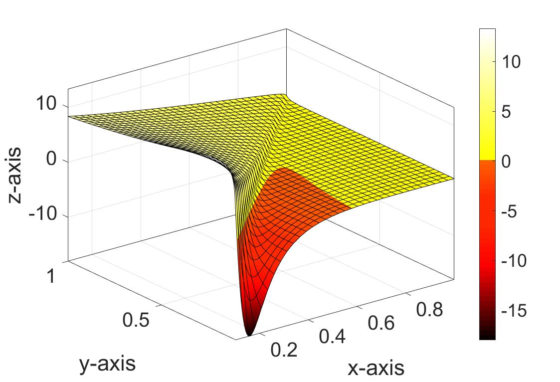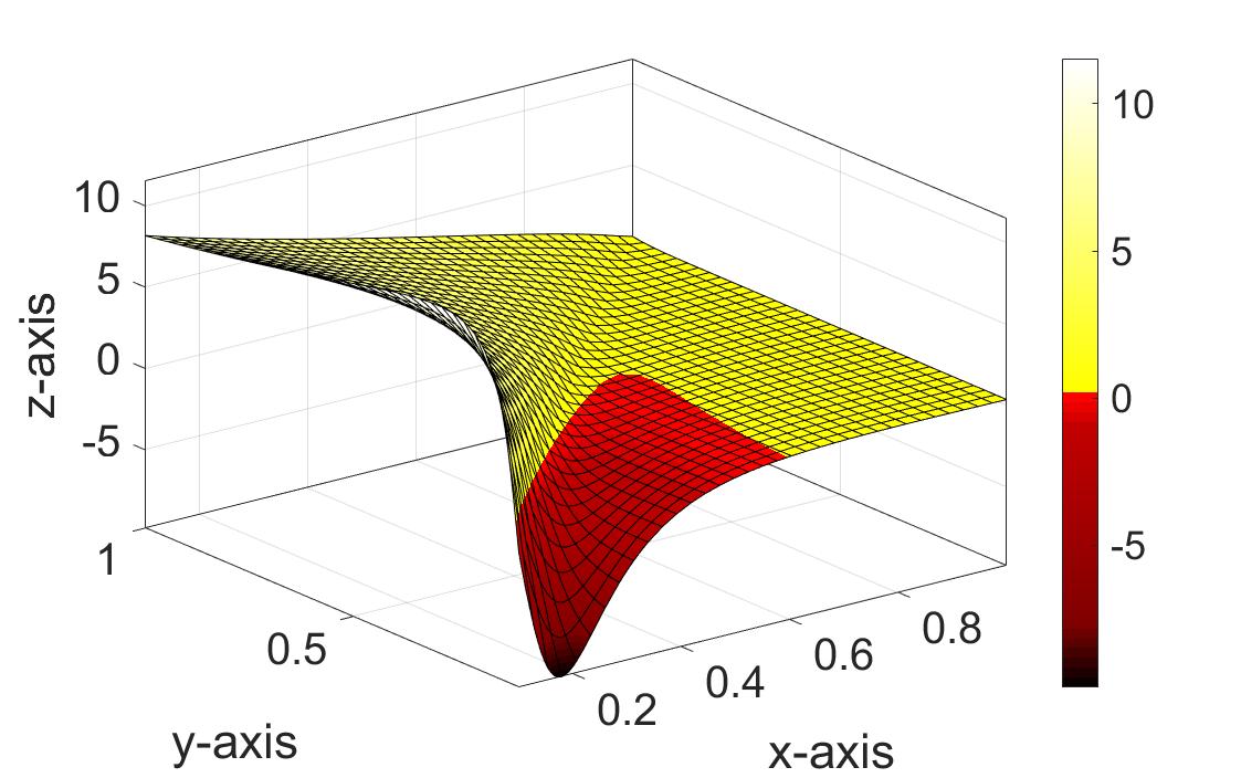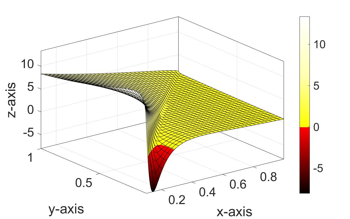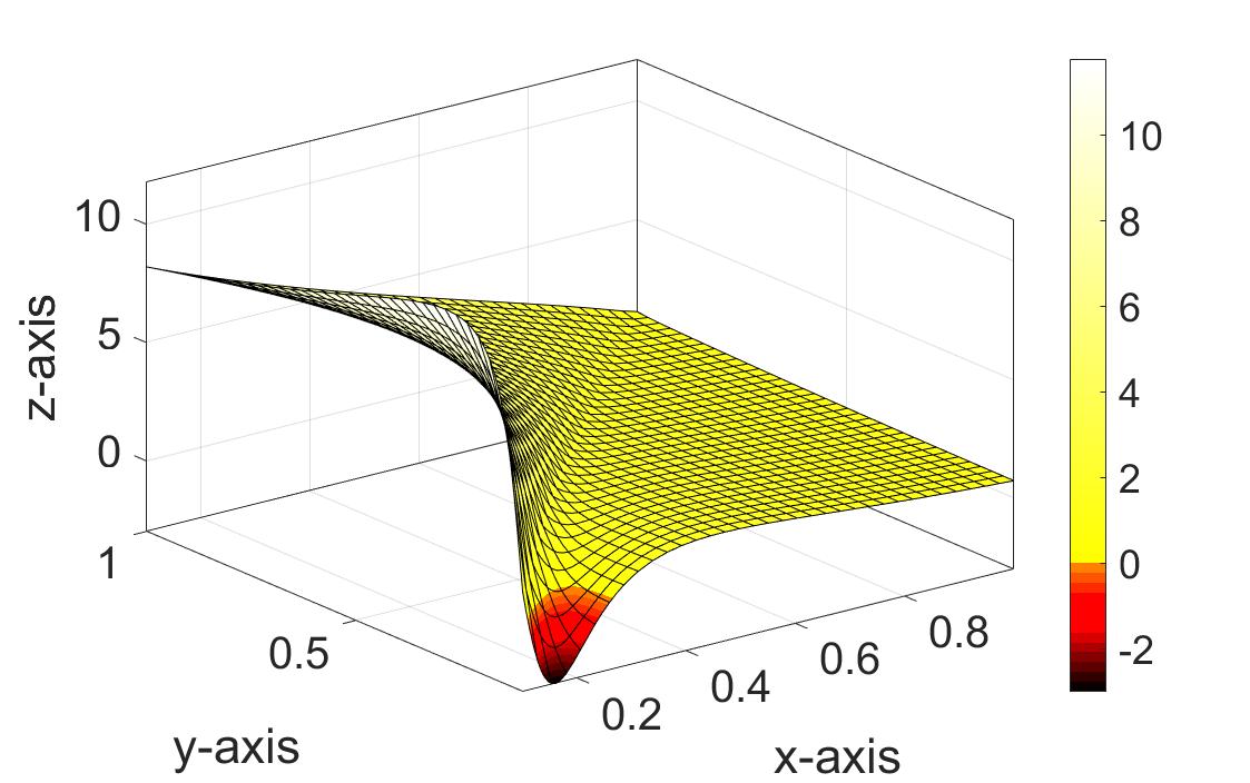Taking into account quadratic terms of the expansion of $\mathcal{F}\left[b,b_{1}\right]$ in $b_{1}$ leads to a screening of the ‘inter-instanton interaction’ and it is also taken into account in Fig. 1(a-d).

The dependence of $S=\Delta F/\left(2mTV\right)$ on parameters characterizing the energy spectrum in SFMOHS is represented in Figs. 1(a-d). Computation of the free energy is performed choosing

$$\varepsilon_{1}\left(\mathbf{p}\right)=\alpha p_{x}^{2}-\beta p_{y}^{2}+P-\mu,\quad\varepsilon_{2}\left(\mathbf{p}\right)=\alpha p_{y}^{2}-\beta p_{x}^{2}-P-\mu$$

corresponding to the spectrum of cuprates near the middle of the edges of the Brillouin zone (momenta $\mathbf{p}$ are counted from the middle of the edges), where $P$ is a Pomeranchuk order parameter obtained previously in SFMOHS volkov1 , and $\mu$ is the chemical potential. We use a parameter $a=U_{\mathrm{0}}/\tilde{U}_{\mathrm{0}},$ and an energy cutoff $\Lambda$ determining the boundary of the hot spots,

$$a=U_{0}/\tilde{U}_{0},\quad\quad\left(\alpha+\beta\right)\left(p_{x}^{2}+p_{y}^{2}\right)/2<\Lambda.$$

Figs. 1 show dependence of $z=2\pi^{2}\left(\alpha+\beta\right)S/\Lambda$ on $x=P/\gamma$ and $y=\Lambda/\gamma$,

(a) $k=0.99$, $a=0$

(b) $k=0.90$, $a=0$

(c) $k=0.99$, $a=1$

(d) $k=0.90$, $a=1$

Figure 1: (Color online.) Free energy of instanton-antiinstanton pairs.

and demonstrate existence of a region of parameters where the free energy $\Delta F$ is negative and the static state is unstable. The region of small $1-k$ and $a$ is most favorable for the formation of the lattice of IAP. As we consider here structures periodic in space (oscillations with vector $\mathbf{Q}_{AF}$ connecting the bands $1$ and $2$), the periodic in $\tau$ order parameter $b\left(\tau\right)$ providing the minimum of the free energy is at the same time the amplitude of the periodic oscillations in space. The present consideration does not determine the number of the pairs $m$ as a function of temperature, and a more accurate study remains to be performed in the future. Below we calculate physical quantities without specifying the value of $m$.

The periodic structure described by the Jacobi elliptic function $b_{0}\left(\tau\right)$ (11) is actually double periodic in the complex plane of $\tau$ and, hence, is periodic in real time $t.$ Remarkably, $b_{0}\left(it\right)$ still satisfies Eq. (10) after the rotation $\tau\rightarrow it.$ Generally, real-time correlation functions can be calculated using a similar technique as previously. At $T=0$ one should replace in Eq. (5) $\tau\rightarrow it$ and integrate over $t$ from $-\infty$ to $\infty.$ Repeating the steps made within the imaginary-time representation one should integrate over functions $B\left(t\right),$ $B_{1}\left(t\right),$ instead of $b\left(\tau\right),$ $b_{1}\left(\tau\right).$ Proceeding in this way one obtains formulas similar to Eqs. (5, 7, 8) but written in real time $t.$ One can prove that the order parameters $B\left(t\right)$ and $B_{1}\left(t\right)$ are related to $b\left(\tau\right)$ and $b_{1}\left(\tau\right)$ as SM ; efetovPRB

$$iB\left(t\right)=b\left(it\right),\quad B_{1}\left(t\right)=b_{1}\left(it\right).$$ (19)

If $B\left(t\right)$ and $B_{1}\left(t\right)$ provide the extremum of the action, the same do $B\left(t-t_{0}\right)$ and $B_{1}\left(t-t_{0}\right)$ for an arbitrary shift $t_{0}.$ Due to this degeneracy one should average over $t_{0}$ at the end of calculations. Physically relevant correlations of the loop currents in the model considered are described exactly by $2$-times correlation function

$$N\left(t\right)=\frac{U_{0}^{2}}{V^{2}}\sum_{p,p^{\prime}}\left\langle\left(c_{p}^{+}\left(t\right)\Sigma_{2}c_{p}\left(t\right)\right)\left(c_{p^{\prime}}^{+}\left(0\right)\Sigma_{2}c_{p^{\prime}}\left(0\right)\right)\right\rangle.$$ (20)

Using the saddle point equations (7, 8), replacing $\tau\rightarrow it$, and using Eq. (19) we obtain in the limit $V\rightarrow\infty$

$$N\left(t\right)=\overline{B\left(t-t_{0}\right)B\left(-t_{0}\right)},$$ (21)

where the bar stands for averaging over $t_{0}.$ One can generally expect a periodic time-dependence of $N\left(t\right)$ using exact solutions for $B\left(t\right).$ It is not easy to find them analytically but we show in Sec. V of Ref. efetovPRB that they are periodic in time, which guarantees the periodicity of the function $N\left(t\right).$ The averaged order parameter vanishes

$$\overline{B\left(t-t_{0}\right)}=0.$$ (22)

Now we approximate, as it was done previously, the function $B\left(t\right)$ by a function $B_{0}\left(t\right)=-ib_{0}\left(it\right)$ and use Eq. (11). The Jacobi elliptic function $\mathrm{sn}\left(iu,k\right)$ of an imaginary argument $iu$ is related to an elliptic function $\mathrm{sc}\left(u|k\right)$ with the period $2K\left(k\right)$ as

$$\mathrm{sn}\left(iu|k\right)=i\mathrm{sc}\left(u|k^{\prime}\right),\;k^{2}+k^{\prime 2}=1,$$

and we write $B\left(t\right)$ in Eq. (21) in the form

$$B\left(t\right)\approx B_{0}\left(t\right)=\gamma k\mathrm{sc}\left(\gamma\left(t-t_{0}\right)|k^{\prime}\right),$$ (23)

Function $N\left(t\right)$, Eq. (21), can be calculated using a Fourier series for the function $\mathrm{sc}\left(u|k\right)$ as . Integration over $t_{0}$ gives in the limit $1-k\ll 1$ $1-k\ll 1$ SM ; efetovPRB

$$N\left(t\right)\approx 2\gamma^{2}\sum_{n=1}^{\infty}f_{n}^{2}\cos\left(2\gamma nt\right),\quad f_{n}=\left[1-\frac{1}{2}\left(\frac{1-k}{8}\right)^{2n}\right].$$

Function $N\left(t\right)$ shows an oscillating behavior with the frequencies $2\gamma n$. The energy $2\gamma$ is the energy of the breaking of electron-hole pairs, and one can interpret the form of $N\left(t\right)$ as oscillations between the static order and normal state. The oscillations of $N\left(t_{1}-t_{2}\right)$ resemble those of the order parameter in the non-equilibrium superconductors vk ; spivak ; barankov ; altshuler ; altshuler1 ; dzero ; galitski ; moor but now the function $N\left(t\right)$ does not decay in time. The contribution of high harmonics $n$ does not decay with $n$ but apparently this is a consequence of the approximation (23) for $B\left(t\right)$. At the same time, one can generally expect a periodic time-dependence of $N\left(t\right)$ using exact solutions for $B\left(t\right).$ It is not easy to find them analytically but one can show that they are periodic in time (Sec. V of Ref. efetovPRB ), which guarantees the periodicity of the function $N\left(t\right).$

The order parameter $B\left(t-t_{0}\right)$ appears when calculating fermionic quantum averages corresponding to the loop currents, and Eq. (22) demonstrates that physical currents are equal to zero at any time $t$. Non-vanishing oscillations of two-times correlation function $N\left(t\right)$ allow us to classify the physical state found here as thermodynamic quantum time-space crystal.

The correlation function $N\left(t\right)$, Eq. (21), was calculated integrating over the position $t_{0}.$ Remarkably, the same results for correlation functions can be obtained considering a Hamiltonian $\hat{H}_{TC}$  of a harmonic oscillator

$$\hat{H}_{TC}=2\gamma\left(a^{+}a+1/2\right),$$ (24)

where $a^{+}$ and $a$ are boson creation and annihilation operators (for simplicity, we consider here the limit $1-k\ll 1$), and an ‘operator order parameter’ $A.$ Using the Hamiltonian $\hat{H}_{TC}$ one can write the correlation function $N\left(t_{1}-t_{2}\right)$ in the form

$$N\left(t\right)=\gamma^{2}\left(\left\langle 0\left|A\left(t\right)A^{+}\left(0\right)\right|0\right\rangle+\left\langle 0\left|A\left(0\right)A^{+}\left(t\right)\right|0\right\rangle\right),$$

where

$$A^{+}\left(t\right)=e^{i\hat{H}_{TC}t}A^{+}e^{-i\hat{H}_{TC}t},\;A^{+}=\sum_{n=1}^{\infty}f_{n}\frac{\left(a^{+}\right)^{n}}{\sqrt{n!}}$$

and $\left|0\right\rangle$ stands for the wave function of the ground state of the Hamiltonian $\hat{H}_{TC}$ (24). At the same time, quantum averages of the operators $A$ and $A^{+}$ vanish

$$\left\langle 0\left|A\left(t\right)\right|0\right\rangle=\left\langle 0\left|A^{+}\left(t\right)\right|0\right\rangle=0.$$

The operator order parameters extends the variety of conventional order parameters like scalars, vectors, matrices used in theoretical physics. The non-decaying time oscillations is an important property for designing qubits.

Possibility of an experimental observation depends on systems described by the Hamiltonian (Thermodynamic quantum time crystals.). For cuprates, inelastic polarized neutron spectroscopy can be a proper tool for observations. Calculating the Fourier transform $N\left(\omega\right)$ of the function $N\left(t\right)$ and comparing it with the one for the hypothetical time-independent DDW result $2\pi\gamma^{2}\delta\left(\omega\right)$, one can write at low temperatures the ratio of the responses at $\left(\pi,\pi\right)$ for these two states as

$$\chi\left(\omega,\mathbf{q}\right)=\chi_{0}\sum_{n=1}^{\infty}f_{n}\delta\left(\omega-2n\gamma\right)\delta\left(\mathbf{q-Q}_{AF}\right),$$ (25)

where $\chi_{0}$ determines the response $\chi_{DDW}$ of the DDW state, $\chi_{DDW}\left(\omega\right)=\chi_{0}\delta\left(\omega\right).$ According to Eq. (25) elastic scattering cannot lead to any signal expected for DDW. Actually, anisotropic magnetic $\left(\pi,\pi\right)$ excitations have been observed hayden in $YBa_{2}Cu_{3}O_{6.9}$ but more detailed experiments are necessary to clarify their origin.

The main conclusion of the present study is that the quantum time-space crystals may exist as a thermodynamically stable state in macroscopic systems. The order parameter of TQTC is periodic in both real and imaginary times but its average over the phase of the oscillations vanishes. The non-decaying oscillations can be seen, e.g., in two- or more times correlation functions. This leads to a natural generalization of the notion of the space long-range order to the time-space one. Two-times correlation functions determine cross-section in inelastic scattering experiments. The frequency of the oscillations remains finite in the limit of infinite volume, $V\rightarrow\infty$. One can expect various experimental consequences and, in particular, one can suppose that the time crystal may be a good candidate for the pseudogap state in superconducting cuprates.

I Supplemental Material to ‘Thermodynamic quantum time crystals’ by Konstantin B. Efetov.

I.1 Free energy.

I.1.1 General scheme of the calculations.

The free energy can be calculated minimizing the free energy functional $\mathcal{F}\left[b,b_{1}\right]$, Eqs. (5, 6), with respect to $b\left(\tau\right)$ and $b_{1}\left(\tau\right)$, which leads to Eqs. (7, 8), and calculating $\mathcal{F}\left[b,b_{1}\right]$ at the minimum. Apparently, exact solutions of Eqs. (7, 8) can be found only numerically, which is beyond the scope of the present publication. As concerns the analytical study, we proceed by introducing eigenfunctions $\Psi_{s\mathbf{p}}\left(\tau\right)$, their conjugates $\bar{\Psi}_{s\mathbf{p}}\left(\tau\right),$ and eigenenergies $\epsilon_{s\mathbf{p}},$ satisfying equations

$$\left(h\left(\tau,\mathbf{p}\right)-i\Sigma_{1}b_{1}\left(\tau\right)\right)\Psi_{s\mathbf{p}}\left(\tau\right) = \epsilon_{s\mathbf{p}}\Psi_{s\mathbf{p}}\left(\tau\right),$$ (26)

$$\bar{\Psi}_{s\mathbf{p}}\left(\tau\right)\left(\bar{h}\left(\tau,\mathbf{p}\right)-i\Sigma_{1}b_{1}\left(\tau\right)\right) = \epsilon_{s\mathbf{p}}\bar{\Psi}_{s\mathbf{p}}\left(\tau\right),$$

and antiperiodicity conditions

$$\Psi_{s\mathbf{p}}\left(\tau+1/T\right)=-\Psi_{s\mathbf{p}}\left(\tau\right),\quad\bar{\Psi}_{s\mathbf{p}}\left(\tau+1/T\right)=-\bar{\Psi}_{s\mathbf{p}}\left(\tau\right).$$ (27)

Operator $h\left(\tau,\mathbf{p}\right)$ has already been introduced in Eq. (6), while its conjugate $\bar{h}\left(\tau,\mathbf{p}\right)$ acting on the left equals

$$\bar{h}\left(\tau,\mathbf{p}\right)=\left(-\overleftarrow{\partial}_{\tau}+\varepsilon^{+}\left(\mathbf{p}\right)-\varepsilon^{-}\left(\mathbf{p}\right)\Sigma_{2}-b\left(\tau\right)\Sigma_{3}\right).$$ (28)

One can introduce a scalar product $\left(,\right)$ and build an orthonormal set of the eigenfunctions

$$\left(\bar{\Psi}_{s\mathbf{p}},\Psi_{s^{\prime}\mathbf{p}}\right)\equiv T\int_{0}^{1/T}\bar{\Psi}_{s\mathbf{p}}\left(\tau\right)\Psi_{s^{\prime}\mathbf{p}}\left(\tau\right)d\tau=\delta_{ss^{\prime}}.$$ (29)

Then, one can write the ‘electronic’ part $\mathcal{F}_{\mathrm{el}}$ (first term in the integrand in Eq. (5)) in the form

$$\frac{\mathcal{F}_{\mathrm{el}}\left[b\left(\tau\right),b_{1}\left(\tau\right)\right]}{VT}=-2\sum_{s}\int\left[\int_{0}^{1/T}\ln\frac{\epsilon_{s\mathbf{p}}}{T}d\tau\right]\frac{d\mathbf{p}}{\left(2\pi\right)^{2}}.$$ (30)

One should keep in mind that the eigenenergies $\epsilon_{s\mathbf{p}}$ are functionals of the functions $b\left(\tau\right)$ and $b_{1}\left(\tau\right).$ The fact that the functional $\mathcal{F}_{\mathrm{el}}\left[b\left(\tau\right),b_{1}\left(\tau\right)\right]$ can be expressed in terms of only the eigenvalues simplifies calculations. We cannot find $\epsilon_{s\mathbf{p}}$ and $\Psi_{s\mathbf{p}}\left(\tau\right)$ exactly for arbitrary $b_{1}\left(\tau\right)$ and use a perturbation theory for the eigenvalues $\epsilon_{s\mathbf{p}}$. In the zero approximation we put $b_{1}\left(\tau\right)=0$ and find the minimum of the functional

$$\mathcal{F}\left[b\left(\tau\right),0\right]=\mathcal{F}_{\mathrm{el}}\left[b\left(\tau\right),0\right]+V\int_{0}^{1/T}\frac{b^{2}\left(\tau\right)}{2U_{0}}d\tau,$$ (31)

which leads to equation (10). The latter can be written in the form

$$b\left(\tau\right)=-U_{0}\sum_{s}\frac{\bar{\Psi}_{s\mathbf{p}}^{\left(0\right)}\left(\tau\right)\Sigma_{3}\Psi_{s\mathbf{p}}^{\left(0\right)}\left(\tau\right)}{\epsilon_{s\mathbf{p}}^{\left(0\right)}},$$ (32)

with $\Psi_{s\mathbf{p}}^{\left(0\right)}\left(\tau\right)$ and $\epsilon_{s\mathbf{p}}^{\left(0\right)}$ equal to the eigenfunctions $\Psi_{s\mathbf{p}}\left(\tau\right)$ and eigenvalues $\epsilon_{s\mathbf{p}}$ taken at $b_{1}\left(\tau\right)=0.$ Solving equations (32, 26) is a non-trivial task even at $b_{1}\left(\tau\right)=0.$ Nevertheless, one can find in this limit $\tau$-dependent solutions exactly, which allows one to calculate $\mathcal{F}\left[b\left(\tau\right),0\right]$ by inserting the eigenvalues $\epsilon_{s\mathbf{p}}^{\left(0\right)}$ and the solution $b\left(\tau\right)$ into Eq. (30).

As the next step, we assume non-zero $b_{1}\left(\tau\right)$, and write

$$b\left(\tau\right)=b_{0}\left(\tau\right)+\delta b\left(\tau\right),$$ (33)

where $b_{0}\left(\tau\right)$ is the solution of Eqs. (32, 26), and expand $\mathcal{F}_{\mathrm{el}}\left[b\left(\tau\right),b_{1}\left(\tau\right)\right],$ Eq. (30), in $b_{1}\left(\tau\right)$ and $\delta b\left(\tau\right)$ up to the second order in these variables. This allows us to obtain the interaction between the fields $b\left(\tau\right)$ and $b_{1}\left(\tau\right),$ Eq. (13), and take into account a screening of this interaction. The calculation of the free energy functional $\mathcal{F}_{\mathrm{el}}\left[b\left(\tau\right),b_{1}\left(\tau\right)\right]$ is done by substituting

$$\epsilon_{s\mathbf{p}}=\epsilon_{s\mathbf{p}}^{\left(0\right)}+\epsilon_{s\mathbf{p}}^{\left(1\right)}+\epsilon_{s\mathbf{p}}^{\left(2\right)},$$ (34)

into Eq. (30) and calculating $\epsilon_{s\mathbf{p}}^{\left(1\right)}$ and $\epsilon_{s\mathbf{p}}^{\left(2\right)}$ with the help of standard quantum-mechanical formulas

$$\epsilon_{s\mathbf{p}}^{\left(1\right)}=-\int_{0}^{1/T}\Pi_{ss}\left(\tau\right)d\tau,\quad\epsilon_{\mathbf{p}}^{\left(2\right)}=\sum_{s^{\prime}\neq s}\int_{0}^{1/T}\frac{\Pi_{ss^{\prime}}\left(\tau\right)\Pi_{s^{\prime}s}\left(\tau\right)}{\epsilon_{s\mathbf{p}}^{\left(0\right)}-\epsilon_{s^{\prime}\mathbf{p}}^{\left(0\right)}}d\tau,$$ (35)

where

$$\Pi_{ss^{\prime}}\left(\tau\right)=\bar{\Psi}_{s\mathbf{p}}^{\left(0\right)}\left(\tau\right)\left(ib_{1}\left(\tau\right)\Sigma_{1}+\delta b\left(\tau\right)\Sigma_{3}\right)\Psi_{s^{\prime}\mathbf{p}}^{\left(0\right)}\left(\tau\right).$$

As soon as the electronic part is calculated, one should minimize $\mathcal{F}\left[b\left(\tau\right),b_{1}\left(\tau\right)\right],$ Eq. (5), with respect to $b_{1}\left(\tau\right)$ and $\delta b\left(\tau\right),$ and calculate the free energy in terms of the solution $b_{0}\left(\tau\right)$ of Eq. (32).

I.1.2 Unperturbed eigenfunctions $\Psi_{s\mathbf{p}}^{\left(0\right)}\left(\tau\right)$ and eigenenergies $\epsilon_{s\mathbf{p}}^{\left(0\right)}$.

Following the proposed scheme we start our calculations by solving Eqs. (26, 32). In order to avoid complicated mathematics one can simply guess the solution $b_{0}\left(\tau\right)$ in the form of Eq. (11). This type of solutions has been used long ago for one dimensional models of polymers brazovskii ; machida ; mertsching , and more recently in Refs. mukhin ; mukhin1 ; mukhin2 for searching imaginary-time-dependent solutions for order parameter.

Function $b_{0}\left(\tau\right)$, Eq. (11), satisfies the following equation

$$\dot{b}_{0}^{2}\left(\tau\right)=b_{0}^{4}\left(\tau\right)-\gamma^{2}\left(1+k^{2}\right)b_{0}^{2}\left(\tau\right)+\gamma^{4}k^{2}.$$ (36)

At $b_{1}\left(\tau\right)=0$ we have instead of Eq. (26) somewhat simpler equations

$$\left(\partial_{\tau}+\varepsilon^{+}\left(\mathbf{p}\right)-\varepsilon^{-}\left(\mathbf{p}\right)\Sigma_{2}-b_{0}\left(\tau\right)\Sigma_{3}\right)\Psi_{s\mathbf{p}}^{\left(0\right)}\left(\tau\right)=\epsilon_{s\mathbf{p}}^{\left(0\right)}\Psi_{s\mathbf{p}}^{\left(0\right)}\left(\tau\right),$$

$$\bar{\Psi}_{s\mathbf{p}}^{\left(0\right)}\left(\tau\right)\left(-\overleftarrow{\partial}_{\tau}+\varepsilon^{+}\left(\mathbf{p}\right)-\varepsilon^{-}\left(\mathbf{p}\right)\Sigma_{2}-b_{0}\left(\tau\right)\Sigma_{3}\right)=\epsilon_{s\mathbf{p}}^{\left(0\right)}\bar{\Psi}_{s\mathbf{p}}^{\left(0\right)}\left(\tau\right).$$ (37)

Solutions $\Psi_{mn\mathbf{p}}^{\left(0\right)}\left(\tau\right)$, $\bar{\Psi}_{mn\mathbf{p}}^{\left(0\right)}\left(\tau\right)$ of Eqs. (37) and the eigenvalues $\epsilon_{s\mathbf{p}}^{\left(0\right)}$ have been found exactly and further used for calculation of $\epsilon_{s\mathbf{p}}$ with the help of Eqs. (35) in Ref. efetovPRB .

I.1.3 Final formulas for the free energy.

Using the eigenfunctions $\Psi_{s\mathbf{p}}^{\left(0\right)}\left(\tau\right)$ and eigenenergies $\epsilon_{\mathbf{p}}^{\left(0\right)}$ obtained in Ref. efetovPRB one can reduce Eqs. (10, 32) to a simpler form

$$1=\frac{U_{0}}{2}\int\Big{[}\tanh\frac{\kappa_{\mathbf{p}}+\varepsilon_{\mathbf{p}}^{+}/T}{2}+\tanh\frac{\kappa_{\mathbf{p}}-\varepsilon_{\mathbf{p}}^{+}/T}{2}\Big{]}$$ (38)

$$\times\frac{\left|\varepsilon^{-}\left(\mathbf{p}\right)\right|}{\sqrt{\left(\left(\varepsilon^{-}\left(\mathbf{p}\right)\right)^{2}+\gamma^{2}\frac{\left(1-k\right)^{2}}{4}\right)\left(\left(\varepsilon^{-}\left(\mathbf{p}\right)\right)^{2}+\gamma^{2}\frac{\left(1+k\right)^{2}}{4}\right)}}\frac{d\mathbf{p}}{\left(2\pi\right)^{2}},$$

which means that the function $b_{0}\left(\tau\right),$ Eq. (11), is an exact solution of Eqs. (10, 32). In fact, there can be many solutions of Eq. (38) because it contains two unknown parameters $\gamma$ and $k.$ Using the periodicity, Eq. (12), one can determine the modulus $k$ for a given integer $m$. We concentrate here on the limit of low temperatures $T.$ In the limit $T\rightarrow 0$ and $k\rightarrow 1,$ Eq. (38) simplifies to Eq. (18).

The energy $F_{\mathrm{inst}}$ entering Eq. (17) with the subsequent equation has been calculated using Eqs. (30, 5). In the zero approximation in $b_{1}\left(\tau\right)$ it takes the form

$$\frac{F_{\mathrm{inst}}}{V}=-2\sum_{s}\ln\frac{\epsilon_{s\mathbf{p}}^{\left(0\right)}}{T}\frac{d\mathbf{p}}{\left(2\pi\right)^{2}}+\frac{T}{\tilde{U}_{\mathrm{0}}}\int_{0}^{1/T}b_{0}^{2}\left(\tau\right)d\tau.$$ (39)

Then, one should sum over all $s$ numerating eigenstates of Eq. (37) in the first term and integrate over $\tau$ in the second one. The energy $F_{\mathrm{II}}$ is obtained from Eq. (15) integrating over $\tau$. Although both the contributions can be calculated exactly at arbitrary $T$ and $k,$ only simplified formulas obtained in the limit of small $T$ and $k\rightarrow 1$ are displayed here in two equations following Eq. (17).

The free energy functional $\Delta\mathcal{F}\left[b_{1},\delta b\right]$ containing both linear and quadratic terms in $b_{1}\left(\tau\right)$ and $\delta b\left(\tau\right)$ can be calculated using Eqs. (5, 30, 34). It can be represented in the form

$$\Delta\mathcal{F}\left[b_{1},\delta b\right]=F_{\mathrm{inst}}+\mathcal{F}_{\mathrm{int}}\left[b_{1}\right]+\mathcal{F}_{\mathrm{2}}\left[b_{1},\delta b\right]$$ (40)

with $F_{\mathrm{inst}}$, Eq. (39), the linear term $\mathcal{F}_{\mathrm{int}}\left[b_{1}\right]$, Eq. (13), and a quadratic form $\mathcal{F}_{\mathrm{2}}$ of $b_{1}\left(\tau\right)$ and $\delta b\left(\tau\right)$ that can be reduced to the form,

$$\frac{\mathcal{F}_{\mathrm{2}}\left[b_{1},\delta b\right]}{VT} = \int_{0}^{1/T}\Big{[}\left(\mathcal{A}\left(\tau\right)-\frac{\mathcal{C}^{2}}{4\mathcal{B}}\dot{b}_{0}^{2}\left(\tau\right)\right)b_{1}^{2}\left(\tau\right)+\mathcal{B}b_{0}^{2}\left(\tau\right)\left(\delta b\left(\tau\right)-\frac{\mathcal{C}\dot{b}_{0}\left(\tau\right)}{2\mathcal{B}b_{0}\left(\tau\right)}b_{1}\left(\tau\right)\right)^{2}\Big{]}d\tau,$$

where

$$\mathcal{A}\left(\tau\right)=\mathcal{A}_{0}+\frac{\mathcal{A}_{1}}{4}\dot{b}_{0}^{2}\left(\tau\right),$$ (42)

and the constants $\mathcal{A}_{0}$, $\mathcal{A}_{1}$, $\mathcal{B}$ and $\mathcal{C}$ equal

$$\mathcal{A}_{0}\mathcal{=}\left(1+\frac{U_{0}}{\tilde{U}_{0}}\right)\int\frac{1}{\sqrt{\left(\varepsilon^{-}\left(\mathbf{p}\right)\right)^{2}+\gamma^{2}}}\frac{d\mathbf{p}}{\left(2\pi\right)^{2}},\quad\mathcal{B=}\frac{1}{\left(\left(\varepsilon^{-}\left(\mathbf{p}\right)\right)^{2}+\gamma^{2}\right)^{3/2}}\frac{d\mathbf{p}}{\left(2\pi\right)^{2}},$$ (43)

$$\mathcal{A}_{1}=\int\frac{1}{\left(\left(\varepsilon^{-}\left(\mathbf{p}\right)\right)^{2}+\gamma^{2}\right)^{3/2}\left(\left(\varepsilon^{-}\left(\mathbf{p}\right)\right)^{2}+\gamma^{2}\frac{\left(1-k\right)^{2}}{4}\right)}\frac{d\mathbf{p}}{\left(2\pi\right)^{2}},$$ (44)

$$\mathcal{C=}\int\frac{\varepsilon^{-}\left(\mathbf{p}\right)}{\left(\left(\varepsilon^{-}\left(\mathbf{p}\right)\right)^{2}+\gamma^{2}\right)^{3/2}\left(\left(\varepsilon^{-}\left(\mathbf{p}\right)\right)^{2}+\frac{\gamma^{2}\left(1-k\right)^{2}}{4}\right)}\frac{d\mathbf{p}}{\left(2\pi\right)^{2}}.$$ (45)

The minimum of $\mathcal{F}_{\mathrm{2}}\left[b_{1},\delta b\right]$ with respect to $\delta b\left(\tau\right)$ is achieved at

$$\delta b\left(\tau\right)=\frac{\mathcal{C}}{2\mathcal{B}b_{0}\left(\tau\right)}\dot{b}_{0}\left(\tau\right)b_{1}\left(\tau\right).$$ (46)

Then, one finds the minimum value of $\Delta\mathcal{F}\left[b_{1},\delta b\right]$ (40) leading to the energy $\Delta F$

$$\frac{\Delta F}{VT}=\frac{F_{\mathrm{inst}}}{VT}-J^{2}\int_{0}^{1/T}\left[\mathcal{A}_{0}+\frac{1}{4}\left(\mathcal{A}_{1}\mathcal{-}\frac{\mathcal{C}^{2}}{\mathcal{B}_{0}}\right)\dot{b}_{0}^{2}\left(\tau\right)\right]^{-1}\dot{b}_{0}^{2}\left(\tau\right)d\tau.$$ (47)

In Eq. (47) the constant $J$ entering Eq. (13) is given in the limit of low temperatures by the integral

$$J=\frac{1}{2}\int\frac{sgn\left(\varepsilon^{-}\left(\mathbf{p}\right)\right)}{\sqrt{\left(\left(\varepsilon^{-}\left(\mathbf{p}\right)\right)^{2}+\gamma^{2}\frac{\left(1-k\right)^{2}}{4}\right)\left(\left(\varepsilon^{-}\left(\mathbf{p}\right)\right)^{2}+\gamma^{2}\right)}}\frac{d\mathbf{p}}{\left(2\pi\right)^{2}}.$$ (48)

The main contribution to the integral (47) comes from the vicinity of zeros of $b_{0}\left(\tau\right)$. Therefore the integral as well as $F_{\mathrm{inst}}$ is proportional to $2m,$ and one can integrate over the half period of the function $b_{0}\left(\tau\right).$ The free energy $\Delta F$ is also proportional to $2m$ and one can calculate the energy per one instanton replacing $b_{0}\left(\tau\right)$ by $\gamma\tanh\gamma\tau$ and integrating over $\tau$ from $-\infty$ to $\infty.$

Equation (47) can be further simplified introducing a new variable of integration $v=\gamma\tanh\gamma\tau.$ In order to compute the energy $\Delta F$ explicitly one should choose a specific form of the electron spectrum, and an option used here is introduced at the bottom of the p. 3 of the main text. Fig. 1 describes results of the calculations using this spectrum.

I.2 Real-time correlation functions.

Of a special interest is a two-times correlation function $N\left(t\right)$, Eq. (20) of two current operators taken at different real times $t_{1}$, $t_{2},$ $t=t_{1}-t_{2}$ and oscillating in space. For the spin-fermion model with the overlapping hot spots, the Fourier transform of this correlation function is proportional to the cross-section of inelastic neutron scattering at the wave vector $\left(\pi,\pi\right)$. Generally, non-decaying $N\left(t\right)$ can be considered as the long-range order of the time crystal.

Starting with Hamiltonian $\hat{H}$, Eq. (Thermodynamic quantum time crystals.), and assuming that $T=0$ one can write the correlation function $N\left(t\right),$ Eq. (20), of currents at different times $t_{1},$ $t_{2}$ and oscillating in space with the vector $\left(\pi,\pi\right)$ in the form (actually, the correlation function of the currents is proportional to $N\left(t\right),$ and one should write a proper coefficient for comparison with experiments). In Eq. (20) the angular brackets $\left\langle...\right\rangle$ stand for quantum-mechanical averaging over the ground state of the Hamiltonian (Thermodynamic quantum time crystals.), and

$$c_{p}\left(t\right)=e^{i\hat{H}t}c_{p}e^{-i\hat{H}t},\quad c_{p}^{+}\left(t\right)=e^{i\hat{H}t}c_{p}^{+}e^{-i\hat{H}t}.$$ (49)

This is a standard definition of the current correlations in the system in thermodynamic equilibrium. The equivalent functional integration is based on averaging with action $\tilde{S}$ written in real time. This action $\tilde{S}\left[\chi\right]$ can be written in real time $t$ in the form

$$\tilde{S}_{\mathrm{0}}\left[\chi\right]=\tilde{S}_{\mathrm{0}}\left[\chi\right]+\tilde{S}_{\mathrm{int}}\left[\chi\right],$$ (50)

where

$$\tilde{S}_{\mathrm{0}}\left[\chi\right]=\sum_{p}\int_{-\infty}^{\infty}\chi_{p}^{+}\left(t\right)\left(-i\partial_{t}+\varepsilon^{+}\left(\mathbf{p}\right)-\varepsilon^{-}\left(\mathbf{p}\right)\Sigma_{2}\right)\chi_{p}\left(t\right)dt,$$ (51)

and

$$\tilde{S}_{\mathrm{int}}\left[\chi\right]=-\frac{1}{4V}\int_{-\infty}^{\infty}\Big{[}U_{\mathrm{0}}\Big{(}\sum_{p}\chi_{p}^{+}\left(t\right)\Sigma_{3}\chi_{p}\left(t\right)\Big{)}^{2}$$

$$-\tilde{U}_{\mathrm{0}}\Big{(}\sum_{p}\chi_{p}^{+}\left(t\right)\Sigma_{1}\chi_{p}\left(t\right)\Big{)}^{2}\Big{]}dt.$$ (52)

Using Eqs. (52) one can write at $T=0$ the following alternative average instead of Eq. (20)

$$N\left(t\right)=\frac{U_{0}^{2}}{V^{2}}\sum_{\mathbf{p,p}^{\prime}\mathbf{,}\alpha,\alpha^{\prime}}\left\langle\left(\chi_{p}^{+}\left(t\right)\Sigma_{3}\chi_{p}\left(t\right)\right)\left(\chi_{p^{\prime}}^{+}\left(0\right)\Sigma_{3}\chi_{p^{\prime}}\left(0\right)\right)\right\rangle_{\tilde{S}}.$$ (53)

In Eq. (53) the angular brackets denote the following average

$$\left\langle...\right\rangle_{\tilde{S}}=\frac{\int\left(...\right)e^{-i\tilde{S}\left[\chi\right]}D\chi}{\int e^{-i\tilde{S}\left[\chi\right]}D\chi}.$$ (54)

(A rotation in the space of the band numbers $1,2$ has been made when passing from Eq. (20) to Eqs. (52, 53)). In order to calculate the average in Eq. (54) we decouple the interaction with the help of the Hubbard-Stratonovich transformation using auxiliary real $B\left(t\right)$ and $B_{1}\left(t\right)$ fields. This leads us to the electron part of action $\mathcal{S}\left[\chi\,\chi^{+},B,B_{1}\left(t\right)\right]$ containing both fermionic $\chi,\chi^{+}$ and bosonic $B\left(t\right),$ $B_{1}\left(t\right)$ fields

$$\mathcal{S}\left[\chi\,\chi^{+},B,B_{1}\left(t\right)\right]=\int_{-\infty}^{\infty}\chi_{p}^{+}\left(t\right)\mathcal{H}\left(t,\mathbf{p}\right)\chi_{p}\left(t\right)dt$$ (55)

with the operator $\mathcal{H}\left(t,\mathbf{p}\right)$ equal to

$$\mathcal{H}\left(t,\mathbf{p}\right)=-i\partial_{t}+\varepsilon^{+}\left(\mathbf{p}\right)-\varepsilon^{-}\left(\mathbf{p}\right)\Sigma_{2}-i\left(B\left(t\right)\Sigma_{3}+B_{1}\left(t\right)\Sigma_{1}\right).$$ (56)

Then, we integrate over $\chi$ and reduce the full action $S$ to the form

$$S=-\ln\left[\int\exp\left[-i\mathcal{S}\left[B,B_{1}\right]\right]DBDB_{1}\right],$$ (57)

where the action functional $\mathcal{S}\left[B,B_{1}\right]$ equals

$$\mathcal{S}\left[B,B_{1}\right] = \int_{-\infty-}^{\infty}\Big{[}-2\sum_{\mathbf{p}}\mathrm{tr}\left[\ln\left(\mathcal{H}\left(\tau,\mathbf{p}\right)\right)\right]_{t,t}$$

$$-V\left(\frac{B^{2}\left(t\right)}{U_{\mathrm{0}}}-\frac{B_{1}^{2}\left(t\right)}{\tilde{U}_{\mathrm{0}}}\right)\Big{]}dt,$$

Minimizing $\mathcal{S}\left[B,B_{1}\right]$ with respect to $B\left(t\right)$ and $B_{1}\left(t\right)$ we come to equations

$$B\left(t\right) = iU_{\mathrm{0}}\mathrm{tr}\int\Sigma_{3}\left[\mathcal{H}^{-1}\left(t,\mathbf{p}\right)\right]_{t,t}\frac{d\mathbf{p}}{\left(2\pi\right)^{2}},$$ (59)

$$B_{1}\left(t\right) = -i\tilde{U}_{\mathrm{0}}\mathrm{tr}\int\Sigma_{1}\left[\mathcal{H}^{-1}\left(t,\mathbf{p}\right)\right]_{t,t}\frac{d\mathbf{p}}{\left(2\pi\right)^{2}}.$$ (60)

Comparing Eqs. (59, 60) with Eqs. (7, 8) we come to conclusion that the functions $B\left(t\right)$ and $B_{1}\left(t\right)$ are related to $b\left(it\right)$ and $b_{1}\left(it\right)$ by Eqs. (19).

It is very important that if $B\left(t\right)$ and $B_{1}\left(t\right)$ are solutions of Eqs. (59, 60), then $B\left(t-t_{0}\right)$ and $B_{1}\left(t-t_{0}\right)$ are also solutions at an arbitrary $t_{0}$. It is also clear that there can be many solutions even at a fixed $t_{0}$. For example, for $B_{1}\left(t\right)=0$ one comes to Eq. (38) for any period of the function $B\left(t\right)$ given by Eq. (23). The relations (19) allow one to obtain proper $B\left(t\right)$ and $B_{1}\left(t\right)$ as soon as $b\left(\tau\right)$ and $b_{1}\left(\tau\right)$ are obtained from the condition for the minimum of the free energy functional $\mathcal{F}\left[b,b_{1}\right]$, Eq. (5).

Now, using Eq. (55, 56) we can integrate over the fermionic fields $\chi,\chi^{+}$ in Eq. (53) to obtain in the limit $V\rightarrow\infty$

$$N\left(t_{1}-t_{2}\right)=-U_{\mathrm{0}}^{2}\overline{\int\mathrm{tr}\left[\Sigma_{3}\mathcal{H}^{-1}\left(t_{1}-t_{0},\mathbf{p}_{1}\right)\right]\frac{d\mathbf{p}_{1}}{\left(2\pi\right)^{2}}\int\mathrm{tr}\left[\Sigma_{3}\mathcal{H}^{-1}\left(t_{2}-t_{0},\mathbf{p}_{2}\right)\right]\frac{d\mathbf{p}_{2}}{\left(2\pi\right)^{2}}},$$ (61)

where the bar stands for the averaging over the period of the structure. Integration over $t_{0}$ is absolutely necessary because the extremum of the action functional is degenerate with the respect to the time shifts, and one should integrate over all the extremum states. Finally, using Eq. (59) we come to Eqs. (21, 23).

References

(1) F. Wilczek, Phys. Rev. Lett.109, 160401 (2012).
(2) P. Bruno, Phys. Rev. Lett.110, 118901 (2013).
(3) F. Wilczek, Phys. Rev.Lett. 110, 118902 (2013).
(4) T. Li, Z.-X. Gong, Z.-Q. Yin, H.T. Quan, X. Yin, P. Zhang,
L.-M. Duan, and X. Zhang, Phys. Rev. Lett. 109, 163001 (2012).
(5) P. Bruno, Phys. Rev. Lett. 111, 029301 (2013).
(6) P. Bruno, Phys. Rev. Lett. 111, 070402 (2013).
(7) P. Nozieres, Europhys. Lett. 103, 57008 (2013).
(8) F. Wilczek, Phys. Rev. Lett. 111, 250402 (2013).
(9) H. Watanabe, and M. Oshikawa, Phys. Rev. Lett. 114, 251603 (2015).
(10) G. Volovik, JETP Lett. 98, 491 (2013).
(11) K. Sacha, Phys. Rev. A 91, 033617 (2015).
(12) V. Khemani, A. Lazarides, R. Moessner, and S.L. Sondhi,
Phys. Rev. Lett. 116, 250401 (2016).
(13) C. W. von Keyserlingk, V. Khemani, and S. L. Sondhi, Phys.
Rev. B 94, 085112 (2016).
(14) D.V. Else, B. Bauer, and C. Nayak, Phys. Rev. Lett. 117, 090402 (2016).
(15) N.Y. Yao, A.C. Potter, I.-D. Potirniche, A. Vishwanath, Phys.
Rev. Lett. 118, 030401 (2017).
(16) S. Autti, V.B. Eltsov, and G. E. Volovik, Phys. Rev. Lett.
120, 215301 (2018).
(17) J. Zhang, P.W. Hess, A. Kyprianidis, P. Becker, A. Lee, J.
Smith, G. Pagano, I.D. Potirniche, A.C. Potter, A. Vishwanath, N.Y. Yao, and
C. Monroe, Nature 543, 217 (2017).
(18) S. Choi, J. Choi, R. Landig, G. Kucsko, H. Zhou, J. Isoya, F.
Jelezko, S. Onoda, H. Sumiya, V. Khemani, C. von Keyserlingk, N.Y. Yao, E.
Demler, and M.D. Lukin, Nature 543, 221 (2017).
(19) P.A. Volkov, and K.B. Efetov, Phys. Rev. B 93,
085131 (2016).
(20) P.A. Volkov, and K.B. Efetov, J. Supercond. Nov. Mag.,
29, 1069 (2016).
(21) P.A. Volkov, and K.B. Efetov, Phys. Rev. B 97,
165125 (2018).
(22) T. Timusk, and B. Statt, Rep. Prog. Phys. 62, 61
(1999).
(23) M.R. Norman, D. Pines, and C. Kallin, Adv. in Phys.,
54, 715 (2005).
(24) M. Hashimoto, I.M. Vishik, Rui-Hua He, T.P. Devereaux,
and Zhi-Xun Shen, Nature Physics 10, 483 (2014).
(25) Supplemental Material
(26) K.B. Efetov, Phys. Rev. B (unpublished); arXiv:1905.04128
(27) J. Bardeen, L.N. Cooper, and J.R. Schrieffer, Phys. Rev.
108, 1175 (1957).
(28) S. Chakravarty, R.B. Laughlin, D.K. Morr, and C.
Nayak, Phys. Rev. B 63, 094503 (2001).
(29) A.F. Volkov, and Sh.M. Kogan, JETP, 38, 1018 (1974).
(30) R.A. Barankov, L.S. Levitov, and B.Z. Spivak, Phys. Rev.
Lett. 93, 160401 (2004).
(31) R.A. Barankov, and L.S. Levitov, Phys. Rev. Lett. 96, 230403 (2006).
(32) E.A. Yuzbashyan, B.L. Altshuler, V.B. Kuznetsov, and
V.Z. Enolskii, Phys. Rev. B 72, 220503(R) (2005).
(33) E.A. Yuzbashyan, O. Tsyplyatyev, and B.L. Altshuler,
Phys. Rev. Lett. 96, 097005 (2006).
(34) E.A. Yuzbashyan, and M. Dzero, Phys. Rev. Lett. 96,
230404 (2006).
(35) V. Galitski, Phys. Rev. B 82, 054511 (2010).
(36) A. Moor, A.F. Volkov, and K.B. Efetov, Phys. Rev. Lett.
118, 047001 (2017).
(37) R. Matsunaga, Y. I. Hamada, K. Makise, Y. Uzawa, H.
Terai, Zhen Wang, and R. Shimano, Phys. Rev. Lett. 111, 057002
(2013).
(38) R.Matsunaga, N. Tsuji, H. Fujita, A. Sugioka, K.
Makise, Y. Uzawa, H. Terai, Z. Wang, H. Aoki, R. Shimano, Science 345, 1145 (2014).
(39) A.A. Abrikosov, L.P. Gorkov, and I.E. Dzyaloshinskii. Methods of quantum field theory in statistical physics. Prentice Hall, New
York (1963).
(40) S.I. Mukhin, J. Supercond. Nov. Mag. 22, 75 (2009).
(41) S.I. Mukhin, J. Supercond. Nov. Mag. 24, 1165
(2011).
(43) M. Abramowitz, and A. Stegun. Handbook of mathematical
functions. Dover, New York (1970).
(44) N.S. Headings, S.M. Hayden, J. Kulda, N.H. Babu, and D.A.
Cardwell, Phys. Rev. B 84, 104513 (2011).
(45) S.A. Brazovskii, S.A. Gordyunin & N.N. Kirova. An
exact solution of the Peierls model with an arbitrary number of electrons in
the unit cell. JETP Lett. 31, 487 (1980).
(46) K. Machida, & M. Fujita. Soliton lattice structure of
incommensurate spin-density wolves: Application to and -rich - and - alloys. Phys. Rev. B 30, 5284 (1984)
(47) J. Mertsching, & H.J. Fischbeck. The Incommensurate
Peierls phase of the quasi-one-dimensional Frohlich model with a nearly
half-filled band. Phys. Stat. Sol. 103, 783 (1981).
(49) P.G. De Gennes, Superconductivity of metals and
alloys. Addison-Wesley, New York (1989).
(50) G. Floquet, Ann. de l’Ecole Norm. Sup. 12, 47