Difficulties in operator-based formulation of the bulk quadrupole moment

Abstract

Electric multipole moments are the most fundamental properties of insulating materials. However, the general formulation of bulk multipoles has been a long standing problem. The solution for the electric dipole moment was provided decades ago by King-Smith, Vanderbilt, and Resta. Recently, there have been attempts at generalizing Resta’s formula to higher-order multipoles. We point out several issues in the recent proposals.

I Introduction

Electric multipole moments are of fundamental importance in understanding the property of insulators. Most significantly, they characterize the charge distribution near boundaries of a finite sample. For two dimensional systems, boundaries can be either one-dimensional edges or zero-dimensional corners. A nonzero electric polarization results in nonzero charge density for edges. Recently, so-called quadrupole insulators that feature charged corners instead of edges have attracted extensive research interest because of their relation to higher-order topological insulators. Parameswaran and Wan (2017); Schindler et al. (2018); Peng et al. (2017); Langbehn et al. (2017); Song et al. (2017); Benalcazar et al. (2017a, b); Fang and Fu (2017); Ezawa (2018); Shapourian et al. (2018); Zhu (2018); Yan et al. (2018); Wang et al. (2018a, b); Khalaf et al. (2018); Khalaf (2018); Trifunovic and Brouwer (2019); Okuma et al. (2018) To develop a systematic understanding of quadrupole insulators, we need to establish a general framework that allows us to compute the quadrupole moment of insulators.

Despite their importance, the precise formulation of multipole moments is known to be a difficult task. For finite systems under the open boundary condition (OBC), multipole moments can be simply defined by the classical formula Resta and Vanderbilt (2007); Lines and Glass (2001); Kittel (2004):

$$n^{\text{(OBC)}}\equiv\frac{1}{V}\sum_{\bm{x}}\langle\Phi_{0}|\hat{n}_{\bm{x}}|\Phi_{0}\rangle,$$ (1)

$$p_{i}^{\text{(OBC)}}\equiv\frac{1}{V}\sum_{\bm{x}}x_{i}\langle\Phi_{0}|\hat{n}_{\bm{x}}|\Phi_{0}\rangle,$$ (2)

$$q_{ij}^{\text{(OBC)}}\equiv\frac{1}{V}\sum_{\bm{x}}x_{i}x_{j}\langle\Phi_{0}|\hat{n}_{\bm{x}}|\Phi_{0}\rangle.$$ (3)

Here, $|\Phi_{0}\rangle$ is the many-body ground state, $\hat{n}_{\bm{x}}$ is the number density operator at the position $\bm{x}$, and $V=L^{2}$ is the volume of the system. (Throughout this work, we consider a two dimensional square-shaped system for brevity.) The polarization $p_{i}^{\text{(OBC)}}$ is independent of the arbitrary choice of the origin only in neutral systems ($n^{\text{(OBC)}}=0$). Similarly, the quadrupole moment $q_{ij}^{\text{(OBC)}}$ is well-defined only when all of $p_{i}^{\text{(OBC)}}$ ($i=x,y$) and $n^{\text{(OBC)}}$ vanish.

The situation gets a lot more complicated when considering extended systems under a periodic boundary condition (PBC), since the position operator in the above expressions becomes ill-defined. Martin (1974); Aligia and Ortiz (1999) For band insulators, King-Smith and Vanderbilt formulated the bulk polarization in terms of the Berry phase of Bloch wavefunctions.Vanderbilt and King-Smith (1993); King-Smith and Vanderbilt (1993) The Berry phase approach was generalized to many-body systems with interactions and/or disorders by replacing the single-particle crystal momentum to the twisted angle of the boundary condition.Ortiz and Martin (1994); Souza et al. (2000); Watanabe and Oshikawa (2018)As an alternative formulation, Resta Resta (1998) proposed the following formula of the bulk electric polarization in many-body setting under a PBC:

$$p_{i}^{\text{(Resta)}}\equiv\frac{1}{2\pi}\text{Im}\ln\langle\Phi_{0}|\hat{U}_{i}|\Phi_{0}\rangle\mod 1,$$ (4)

$$\hat{U}_{i}\equiv e^{2\pi i\hat{P}_{i}/L},\quad\hat{P}_{i}\equiv\sum_{\bm{x}}x_{i}\hat{n}_{\bm{x}}.$$ (5)

According to Ref. Resta, 1998, this relation holds even in the presence of disorders and many-body interactions as long as the excitation gap is non-vanishing.

There have been several recent proposals on how to compute the bulk quadrupole moment. For band insulators, the nested-Wilson loop approach formulated in Refs. Benalcazar et al., 2017a, b aims at providing a way of computing the bulk contribution to the quantized corner charge, under assumptions of the spatial symmetry and the so-called “Wannier gap”. We remark here that, although the nested-Wilson loop approach gives a topological invariant, this invariant is generally not a bulk topological invariant—according to Ref. Benalcazar et al., 2017b the nested Wilson loop invariant can change its value if the Wannier gap is closed while the bulk band gap and the protecting symmetry are maintained. Yet, the claim of Refs. Benalcazar et al., 2017a, b is that combining the “bulk” contribution to the edge polarization $p_{x}^{\text{edge}}$, $p_{y}^{\text{edge}}$ obtained this way with an independent input on the corner charge $Q^{\text{corner}}$ computed under a certain open boundary condition, one gets the bulk quadrupole moment via $q_{xy}=Q^{\text{corner}}-p_{x}^{\text{edge}}-p_{y}^{\text{edge}}$. Benalcazar et al. (2017a, b) As later pointed out by us, Trifunovic et al. (2019) decorations by polarized one-dimensional chains change the corner charge; the boundary Hamiltonian and thus the boundary polarization are not generally defined quantities. Therefore it is not possible to subtract the contribution from edge polarization.

As a more general definition of the bulk quadrupole moment in many-body systems under a PBC, two independent groups Wheeler et al. (2018); Kang et al. (2018) proposed a possible generalization of Resta’s formula to higher-order multipoles. For example, their formulas for quadrupole moments read

$$\tilde{q}_{ij}\equiv\frac{1}{2\pi}\text{Im}\ln\langle\Phi_{0}|\hat{U}_{ij}|\Phi_{0}\rangle\mod 1,$$ (6)

$$\hat{U}_{ij}\equiv e^{2\pi i\hat{Q}_{ij}/L^{2}},\quad\hat{Q}_{ij}\equiv\sum_{\bm{x}}x_{i}x_{j}\hat{n}_{\bm{x}}.$$ (7)

Arguments supporting Eq. (6) are based on a field theoretical calculation of the bulk response against a non-uniform electric field Kang et al. (2018) and a “perturbation” theory  expanding the effect of the operator $\hat{U}_{ij}$ in the series of $x_{i}x_{j}/L^{2}$.Wheeler et al. (2018) The authors of Refs. Kang et al., 2018; Wheeler et al., 2018 have also provided a numerical proof of Eq. (6) using tight-binding models of quadrupole insulators. More recently, Refs. Agarwala et al. (2019); Lin et al. (2019) employed the formula (6) in their study of quadrupole insulators.

The goal of this work is to point out issues in the formula (6) for the bulk quadrupole moment. A satisfactory formulation of the bulk quadrupole moment would fulfill the following requirements: (i) independence from the choice of origin and the period $L$ and (ii) quantization in the presence of sufficiently large point group symmetries so that it can serve as a topological invariant characterizing the quantized corner charge of quadrupole insulators. However, we discuss that the operator $\hat{U}_{ij}$ in Eq. (7) is inconsistent with the assumed PBC, and, as a consequence, $\tilde{q}_{ij}$ in Eq. (6) meets none of these criteria.

II Problems in the proposed formula

II.1 Violation of the periodicity

We first point out an obvious issue in Eqs. (6) and (7). Let us consider a single-particle state $|\psi\rangle=\sum_{\bm{x}}\psi(\bm{x})c_{\bm{x}}^{\dagger}|0\rangle$. The PBC requires that the wavefunction $\psi(\bm{x})$ has the periodicity in $\bm{x}$ with the period $L$ in both the $x$ and $y$ directions:

$$\psi(\bm{x}+L\bm{e}_{i})=\psi(\bm{x}).$$ (8)

where $\bm{e}_{i}$ represents the unit vector along $i=x,y$. For example, the wavefunction of the Bloch state $\psi_{\bm{k}n}(\bm{x})=(1/\sqrt{V})u_{\bm{k}n}(\bm{x})e^{i\bm{k}\cdot\bm{x}}$ fulfills this condition thanks to the quantization of $\bm{k}$ to the integer multiples of $2\pi/L$.

The operator $\hat{U}_{i}$ in Eq. (5) preserves this periodicity. The wavefunction of the state $\hat{U}_{i}|\psi\rangle$ is $e^{2\pi ix_{i}/L}\psi(\bm{x})$, which satisfies Eq. (8). In contrast, $\hat{U}_{ij}$ defined in Eq. (7) violates the periodicity. The wavefunction of the state

$$\hat{U}_{ij}|\psi\rangle=\sum_{\bm{x}}e^{2\pi ix_{i}x_{j}/L^{2}}\psi(\bm{x})c_{\bm{x}}^{\dagger}|0\rangle$$ (9)

is not invariant under $\bm{x}\rightarrow\bm{x}+L\bm{e}_{i}$. Thus, $\hat{U}_{ij}|\psi\rangle$ does not belong to the Hilbert space specified by the PBC. Therefore the quantity $\langle\psi|\hat{U}_{ij}|\psi\rangle$ (the inner-product of two states $|\psi\rangle$ and $\hat{U}_{ij}|\psi\rangle$) lacks the physical meaning. Reference Wheeler et al., 2018 proposed to fix this issue by allowing for discontinuities, but then the analyticity of the wavefunction would be lost.

To discuss more general states, let $\hat{T}_{L\bm{e}_{i}}$ be the translation operator that shifts $\bm{x}$ to $\bm{x}+L\bm{e}_{i}$ ($i=x,y$). Imposing the PBC is equivalent to identifying $\hat{T}_{L\bm{e}_{i}}$ with an identity operator. $\hat{U}_{i}$ in Eq. (5) is consistent with this identification because it commutes with $\hat{T}_{L\bm{e}_{i}}$. On the other hand, $\hat{U}_{ij}$ in Eq. (7) does not commute with $\hat{T}_{L\bm{e}_{i}}$ and consequently it violates the boundary condition.

This simple discussion already poses a serious question about the physical meaning of $\tilde{q}_{ij}$ in Eq. (6). Below we discuss the immediate consequence of the lack of periodicity.

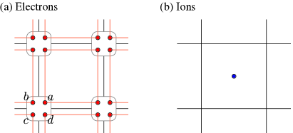
Figure 1: (a) The tight-binding model in Eq. (10) describing the electronic contribution. Orange lines represent hopping. (b) Ions localized at plaquette center.

II.2 Tight-binding example of quadrupole insulator

Here we consider a simplified version of the four-band tight-binding model introduced in Ref. Benalcazar et al., 2019. See Appendix C for more physical tight-binding models. As illustrated in Fig. 1 (a), the model has four orbitals ($a$, $b$, $c$, and $d$) at each lattice site. The Hamiltonian in Fourier space reads

$$H_{\bm{k}}=-\begin{pmatrix}0&e^{ik_{x}}&0&e^{ik_{y}}\\ e^{-ik_{x}}&0&e^{ik_{y}}&0\\ 0&e^{-ik_{y}}&0&e^{-ik_{x}}\\ e^{-ik_{y}}&0&e^{ik_{x}}&0\\ \end{pmatrix}.$$ (10)

We assume $C_{4}$ rotation symmetry to see if $\tilde{q}_{ij}$ is quantized as proposed by Ref. Kang et al., 2018.

$$U_{C_{4}}H_{k_{x},k_{y}}=H_{-k_{y},k_{x}}U_{C_{4}},\quad U_{C_{4}}\equiv\begin{pmatrix}0&0&0&1\\ 1&0&0&0\\ 0&1&0&0\\ 0&0&1&0\\ \end{pmatrix}.$$ (11)

We write the position of lattice sites as $\bm{R}=(x_{n},y_{m})$, where $x_{n}=x_{1}+n-1$ and $y_{m}=x_{1}+m-1$ ($n,m=1,2,\ldots,L$). The lattice constant is set to be unity for simplicity. Here, $x_{1}$ is introduced to investigate the origin dependence of the results.  Below we consider two familiar choices of $x_{1}$: $x_{1}=1$ ($x_{L}=L$) for every $L$ and $x_{1}=-(L-1)/2$ ($x_{L}=-x_{1}$) for an odd $L$.

The four eigenvalues of $H_{\bm{k}}$ are $0$ (doubly degenerate) and $\pm 2$. The Bloch function of the lowest band ($\varepsilon_{\bm{k}}=-2$) reads $u_{\bm{k}}=(1,e^{-ik_{x}},e^{-i(k_{x}+k_{y})},e^{-ik_{y}})^{T}/2$. In the Wannier basis, the ground state that completely occupies the lowest band can be written $|\Phi_{0}\rangle=\prod_{\bm{R}}\hat{\gamma}_{\bm{R}}^{\dagger}|0\rangle$ with

$$\hat{\gamma}_{\bm{R}}^{\dagger}\equiv\frac{1}{2}(\hat{c}_{\bm{R}a}^{\dagger}+\hat{c}_{\bm{R}+\bm{e}_{x},b}^{\dagger}+\hat{c}_{\bm{R}+\bm{e}_{x}+\bm{e}_{y},c}^{\dagger}+\hat{c}_{\bm{R}+\bm{e}_{y},d}^{\dagger}).$$ (12)

Using this real space expression, one can analytically evaluate $\tilde{q}_{ij}$. We present the detailed calculation in Appendix B.

Next we consider ionic contributions. To cancel the electric charge and polarization, we place an ion at every plaquette center, i.e. $\bm{x}=\bm{R}+(\bm{e}_{x}+\bm{e}_{y})/2$ as illustrated in Fig. 1 (b). $\tilde{q}_{ij}$ in Eq. (6) for ions reduces to

$$\tilde{q}_{ij,\text{ions}}=\frac{1}{L^{2}}\sum_{\bm{R}}\left(R_{i}+\frac{1}{2}\right)\left(R_{j}+\frac{1}{2}\right).$$ (13)

We subtract this reference value from the electronic contribution to impose the charge neutrality and vanishing polarization.

$$\Delta p_{i}^{\text{(Resta)}}=p_{i}^{\text{(Resta)}}-p_{i,\text{ions}}^{\text{(Resta)}}=0,$$ (14)

$$\Delta\tilde{q}_{ij}=\tilde{q}_{ij}-\tilde{q}_{ij,\text{ions}}.$$ (15)

We summarize our results in Table 1. We immediately realize that the value of $\Delta\tilde{q}_{ij}$ depends sensitively on the detailed choice of origin [compare $x_{1}=1$ and $x_{1}=-(L-1)/2$ for an odd $L$] and also on the parity of $L$ [compare the even and odd $L$ for $x_{1}=1$]. Also, the value of $\Delta\tilde{q}_{xy}$ is not necessarily quantized [see the case of $x_{1}=1$ with an even $L$].

Table 1: The analytic expression of $\Delta\tilde{q}_{ij}$ for the tight-binding model in Eq. (10) in the limit of large $L$.

$\,\,\,\,\,\,(x_{1},L)\,\,\,\,\,\,$	$\,\,\,\,\,\,(1,\text{even})\,\,\,\,\,\,$	$\,\,\,\,\,\,(1,\text{odd})\,\,\,\,\,\,$	$\,\,\,\,\,\,(-\frac{L-1}{2},\text{odd})\,\,\,\,\,\,$
$\Delta\tilde{q}_{xx}$, $\Delta\tilde{q}_{yy}$	$\frac{1}{4}$	$\frac{1}{4}$	$\frac{3}{4}$
$\Delta\tilde{q}_{xy}$, $\Delta\tilde{q}_{yx}$	$\frac{1}{2}+\frac{1}{\pi}\arctan\frac{2}{\pi}$	$\frac{1}{2}$	$\frac{3}{4}$

III Difficulties in the improvement

III.1 Absence of Resta’s type formula

Let us ask if one can fix the issues in $\tilde{q}_{ij}$ identified above. Here we explore the Resta-type expression $\tilde{q}^{\prime}\equiv\frac{1}{2\pi}\text{Im}\ln\langle\Phi_{0}|\hat{U}^{\prime}|\Phi_{0}\rangle$ with $\hat{U}^{\prime}\equiv e^{2\pi i\sum_{\vec{x}}\theta_{\vec{x}}\hat{n}_{\vec{x}}}$. To be consistent with the PBC, $\theta_{\vec{x}}$ must have the following form

$$\theta_{\bm{x}}=\frac{m_{x}x+m_{y}y}{L}+\vartheta_{\bm{x}}\quad(m_{i}\in\mathbb{Z}),$$ (16)

where $\vartheta_{\bm{x}}\in\mathbb{R}$ is a periodic function of $\bm{x}$. In particular, quadratic terms such as $x_{i}x_{j}/L^{2}$ cannot appear in $\theta_{\bm{x}}$ contrary to Eq. (7).

One may introduce a cut-off function $C_{\vec{x}}\in[0,1]$ that is $1$ (constant) when $\bm{x}$ is far away from the boundary (i.e., $x_{1}\ll x\ll x_{L}$ and $y_{1}\ll y\ll y_{L}$) and smoothly approaches to $0$ when $\vec{x}$ is near the boundary with an intermediate length scale $\ell$ ($1\ll\ell\ll L$). For example, we can use

$$C_{\vec{x}}= \tfrac{1+\tanh\frac{x-x_{1}-\frac{L}{4}}{\ell}}{2}\tfrac{1-\tanh\frac{x-x_{L}+\frac{L}{4}}{\ell}}{2}$$ (17)

$$\times\tfrac{1+\tanh\frac{y-y_{1}-\frac{L}{4}}{\ell}}{2}\tfrac{1-\tanh\frac{y-y_{L}+\frac{L}{4}}{\ell}}{2}.$$

Then $\vartheta_{\bm{x}}=C_{\bm{x}}\,xy/L^{2}$ becomes effectively a periodic function when terms proportional to $e^{-L/4\ell}$ are neglected. However, we found that such a modification does not resolve the issues, because the contribution to $\tilde{q}^{\prime}$ from the decaying region ($|\partial_{x}C_{\bm{x}}|\sim 1/\ell$) is non-neglegible and spoils the bulk contribution from the interior ($C_{\bm{x}}\simeq 1$).

III.2 Absence of a Berry-phase type formula

Next, let us examine Berry-phase type formulas. According to the modern theory of electric polarization,Vanderbilt and King-Smith (1993); King-Smith and Vanderbilt (1993) the Berry phase

$$\int_{\text{BZ}}\frac{d^{2}k}{(2\pi)^{2}}\sum_{n=1}^{N_{\text{occ}}}i\langle u_{\bm{k}n}|\partial_{k_{i}}u_{\bm{k}n}\rangle$$ (18)

gives the electric polarization. Here, $|u_{\bm{k}n}\rangle$ is the Bloch function of $n$-th occupied band. This Berry phase can be interpreted as the expectation value of the position operator measured from the origin of the unit cell $\int d^{2}x\sum_{n=1}^{N_{\text{occ}}}w_{n\bm{R}}(\bm{x})^{*}(x_{i}-R_{i})w_{n\bm{R}}(\bm{x})$ of the Wannier state $w_{n\bm{R}}(\bm{x})\equiv L^{-2}\sum_{\bm{k}}e^{i\bm{k}\cdot(\bm{x}-\bm{R})}u_{\bm{k}n}(\bm{x})$. Therefore one may guess that the bulk quadrupole is given by $\int d^{2}x\sum_{n=1}^{N_{\text{occ}}}w_{\bm{R}}(\bm{x})^{*}(x_{i}-R_{i})(x_{j}-R_{j})w_{\bm{R}}(\bm{x})$, i.e.,

$$\int_{\text{BZ}}\frac{d^{2}k}{(2\pi)^{2}}\sum_{n=1}^{N_{\text{occ}}}\langle\partial_{k_{i}}u_{\bm{k}n}|\partial_{k_{j}}u_{\bm{k}n}\rangle.$$ (19)

However, this cannot be the case because the quantity in Eq. (19) is not invariant under the gauge transformation $w_{\vec{k}}\in\text{U}(N_{\text{occ}})$ among occupied bands,

$$|u_{\bm{k}n^{\prime}}\rangle^{\prime}=\sum_{n=1}^{N_{\text{occ}}}|u_{\bm{k}n}\rangle(w_{\bm{k}})_{n,n^{\prime}}.$$ (20)

We can fix the gauge-invariance by inserting the projector onto unoccupied bands $1-P_{\bm{k}}$ Marzari and Vanderbilt (1997); Resta and Sorella (1999); Souza et al. (2000)

$$T_{ij}\equiv\int_{\text{BZ}}\frac{d^{2}k}{(2\pi)^{2}}\sum_{n=1}^{N_{\text{occ}}}\langle\partial_{k_{i}}u_{\bm{k}n}|(1-P_{\bm{k}})|\partial_{k_{j}}u_{\bm{k}n}\rangle.$$ (21)

However, we then found that this quantity does not produce a useful topological invariant, because $T_{ij}$ is always proportional to an identity matrix in the presence of $n=3$, $4$, or $6$-fold rotation symmetry. [This is because it satisfies $\sum_{i,j}(p)_{i^{\prime}i}T_{ij}(p^{T})_{jj^{\prime}}=T_{i^{\prime}j^{\prime}}$ under a point group symmetry $p\in\text{O}(2)$.] A useful topological invariant would be constructed from an integral with an integer ambiguity, but, to our knowledge, the Berry phase in Eq. (18) is the only combination with that property in two dimensions.

IV Summary

We have analyzed the definition of the bulk quadrupole moment independently proposed by two groups. Kang et al. (2018); Wheeler et al. (2018) We find that the proposed definition of the bulk quadrupole moment fails even for a simple non-interacting example. Our analysis reveals that the issues with the proposed definition are related to violation of periodicity. Possible strategies to fix these issues all seem to fall short.

The obstacles in obtaining a generalization of Resta’s formulation of bulk polarization to higher multipoles are perhaps best illustrated by our findings that even a simpler task, namely, finding a formulation for single-particle systems seems to fail. Although we cannot provide a general proof that such single-particle formulation of bulk quadrupole moment does not exist, we give a strong indication that this task may be a difficult one.

A proper definition of higher multiples in crystals and formulas that allow practical calculations are topics of broad interest, not limited to computational and theoretical solid state physics. Despite the fact that our findings support in some sense a ‘no-go’ statement, we hope that this work will serve as the first step toward the future resolution to defining bulk multiple moments.

Appendix A Subtlety in the perturbative expansion

Resta Resta (1998) used the “first-order perturbation theory” to derive Eq. (4) for interacting systems. Ref. Wheeler et al., 2018 used a similar perturbative argument to verify the formula (7). Here, we review an issue with such perturbative treatment following Ref. Watanabe and Oshikawa, 2018. Only in this appendix do we assume a general $d$ dimensional system with the period $L_{i}$ in $i$-th direction. According to Resta, Resta (1998)

$$\hat{U}_{x}|\Phi_{0}\rangle\doteq e^{i\gamma}\left(|\Phi_{0}\rangle+\frac{2\pi}{L_{x}}\sum_{N>0}|\Phi_{N}\rangle\frac{\langle\Phi_{N}|\hat{J}_{x}|\Phi_{0}\rangle}{E_{N}-E_{0}}+\cdots\right),$$ (22)

where $\hat{J}_{x}$ is the sum of the $x$-component of the current operators over the entire space. If the above relation were a controlled expansion in the series of $L_{x}^{-1}$, the expectation value $\langle\Phi_{0}|\hat{U}_{x}|\Phi_{0}\rangle$ would behave as

$$|\langle\Phi_{0}|\hat{U}_{x}|\Phi_{0}\rangle|\doteq 1+O(L_{x}^{-2}),$$ (23)

which converges to $1$ in the large $L_{x}$ limit. However, this turns out not to be the case because of the volume sum hidden in $\hat{J}_{x}$. Watanabe and Oshikawa (2018) We put the dot over the equality in Eqs. (22) and  (23) as a caution to the reader.

This issue can be readily seen in the case of band insulators. The matrix element of $\hat{U}_{x}$ among Bloch states is given by

$$(\hat{U}_{x})_{\bm{k}^{\prime}n^{\prime},\bm{k}n}=\delta_{\bm{k}^{\prime},\bm{k}+(2\pi/L_{x})\bm{e}_{x}}(B_{\bm{k}})_{n^{\prime}n},$$ (24)

where $n=1,2,\cdots,N_{\text{occ}}$ is the band index of occupied bands and $B_{\bm{k}}$ is an $N_{\text{occ}}$-dimensional matrix representing the discretized Berry connection defined by

$$(B_{\bm{k}})_{n^{\prime}n} \equiv\langle u_{\bm{k}+(2\pi/L_{x})\bm{e}_{x}n^{\prime}}|u_{\bm{k}n}\rangle.$$ (25)

By expanding $B_{\bm{k}}$ to the second order in $L_{x}^{-1}$, we find

$$|\langle\Phi_{0}|\hat{U}_{x}|\Phi_{0}\rangle|=e^{-2\pi^{2}G_{xx}V/L_{x}^{2}+O(V/L_{x}^{3})},$$ (26)

where $V=L_{x}L_{y}\cdots$ is the volume and $G^{ij}$ is the quantum metric tensor defined by Marzari and Vanderbilt (1997); Resta and Sorella (1999); Souza et al. (2000)

$$G_{ij}\equiv\text{Re}\int\frac{d^{d}k}{(2\pi)^{d}}(g_{\bm{k}})_{ij},$$ (27)

$$(g_{\bm{k}})_{ij}=\sum_{n=1}^{N_{\text{occ}}}\langle\partial_{k_{i}}u_{\bm{k}n}|(1-P_{\bm{k}})|\partial_{k_{j}}u_{\bm{k}n}\rangle.$$ (28)

Note that $G_{ij}=O(1)$, i.e., it does not depend on the system size. For example, for the isotropic case in which all $L_{i}$’s are identical to $L$, the right-hand side of Eq. (26) is $e^{-2\pi^{2}G^{xx}L^{{d-2}}+O(L^{{d-3}})}$. In the large $L$ limit, it converges to a number in the range $0$ and $1$ in two dimension, and it vanishes in higher dimensions. This is in sharp contrast to the behavior in Eq. (23). Thus the first-order perturbation (22) does not hold in general. 

Quite remarkably, despite the lack of a general proof of Eq. (4) for interacting systems in multi-dimensions, to best of our knowledge there is no counterexample to Eq. (4). Unfortunately, as we discuss in the main text, the circumstances are not so favorable for the validity of the proposed expression (7), where a similar perturbative expansion argument was used. Wheeler et al. (2018)

Appendix B Details on the tight-biding calculation

Here we present the derivation of the result for the model in Eq. (10) summarized in Table 1. To compute $\tilde{q}_{ij}$ in Eq. (6), one has to compute the matrix element of $\hat{U}_{ij}$ in Eq. (7) among occupied single-particle states. To this end, working in the Wannier basis instead of the Bloch basis is advantageous, because all the off-diagonal elements [i.e. $(\hat{U}_{ij})_{\bm{R},\bm{R}^{\prime}}$, $\bm{R}\neq\bm{R}^{\prime}$] vanish for the Wannier state in Eq. (12). Because of this nice property, we have

$$\tilde{q}_{ij}=\frac{1}{2\pi}\sum_{\bm{R}}\text{Im}\ln(\hat{U}_{ij})_{\bm{R},\bm{R}}.$$ (29)

The expression for the diagonal matrix element $(\hat{U}_{ij})_{\bm{R},\bm{R}}$ depends on the position of plaquettes, i.e., whether $\bm{R}$ is in the bulk or around the boundary. Introducing the shorthand notation $F_{z}=e^{2\pi iz/L^{2}}$, the diagonal elements can be written as

$$(\hat{U}_{xx})_{\bm{R},\bm{R}}=\frac{1}{2}\times\begin{cases}F_{R_{x}^{2}}+F_{(R_{x}+1)^{2}}&\text{for }R_{x}<x_{L}\\ F_{x_{L}^{2}}+F_{x_{1}^{2}}&\text{for }R_{x}=x_{L}\end{cases},$$ (30)

$$(\hat{U}_{yy})_{\bm{R},\bm{R}}=\frac{1}{2}\times\begin{cases}F_{R_{y}^{2}}+F_{(R_{y}+1)^{2}}&\text{for }R_{y}<y_{L}\\ F_{y_{L}^{2}}+F_{y_{1}^{2}}&\text{for }R_{y}=y_{L}\end{cases},$$ (31)

and

$$(\hat{U}_{xy})_{\bm{R},\bm{R}}=(\hat{U}_{yx})_{\bm{R},\bm{R}}=\frac{1}{4}\times\begin{cases}F_{R_{x}R_{y}}+F_{(R_{x}+1)R_{y}}+F_{(R_{x}+1)(R_{y}+1)}+F_{R_{x}(R_{y}+1)}&\text{for }R_{x}<x_{L}\text{ and }R_{y}<y_{L}\\ F_{x_{L}R_{y}}+F_{x_{1}R_{y}}+F_{x_{1}(R_{y}+1)}+F_{x_{L}(R_{y}+1)}&\text{for }R_{x}=x_{L}\text{ and }R_{y}<y_{L}\\ F_{R_{x}y_{L}}+F_{(R_{x}+1)y_{L}}+F_{(R_{x}+1)y_{1}}+F_{R_{x}y_{1}}&\text{for }R_{x}<x_{L}\text{ and }R_{y}=y_{L}\\ F_{x_{L}y_{L}}+F_{x_{1}y_{L}}+F_{x_{1}y_{1}}+F_{x_{L}y_{1}}&\text{for }R_{x}=x_{L}\text{ and }R_{y}=y_{L}\end{cases}.$$ (32)

To reproduce Table 1, one just has to plug these expressions into Eq. (29) and extract the value in the large $L$ limit.

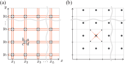
Figure 2: Illustration of the first model (a) and the atomic limit (b).

Appendix C Examples of tight-biding models

In this section, we discuss two tight-binding models that are more physically natural than the simplified one discussed in Sec. II.2. This exercise will support our claim, clarifying the issues in the proposed formula (6).

C.1 Model 1

The first model is illustrated in Fig. 2 (a). As far as the electronic degrees of freedom are concerned, this model is identical to the one in Eq. (10). The only difference is the position of ions. Since lattice sites are located at $\bm{R}=(x_{n},y_{m})$ (see the main text), here we assume that one ion sits at every lattice site $\bm{R}$. This choice gives the reference value

$$\tilde{q}_{xy,\text{ions}} =\frac{(2x_{1}+L-1)^{2}}{4}.$$ (33)

The lowest band of the model (10) has a Wannier orbital centering at $\bm{x}=\bm{R}+(\frac{1}{2},\frac{1}{2})$ for each $\bm{R}$. The band insulator that completely occupies this band has

$$\tilde{q}_{xy}^{\text{(a)}}=\frac{1}{2\pi}\sum_{\bm{R}}\text{Im}\ln(\hat{U}_{xy}^{\text{(a)}})_{\bm{R},\bm{R}},$$ (34)

where $(\hat{U}_{xy}^{\text{(a)}})_{\bm{R},\bm{R}}$ is given in Eq. (32). We tabulate the value of $\Delta\tilde{q}_{xy}^{\text{(a)}}=\tilde{q}_{xy}^{\text{(a)}}-\tilde{q}_{xy,\text{ions}}$ in Table 2.

We compare this to the atomic limit illustrated in Fig. 2 (b). In this limit, all electrons are strictly localized at the Wannier center $\bm{x}=\bm{R}+(\frac{1}{2},\frac{1}{2})$ for every $\bm{R}$. The above band insulator can be adiabatically connected to this limit without closing the bulk gap or breaking the $C_{4}$ symmetry. For the atomic limit, we find

$$(\hat{U}_{xy}^{\text{(b)}})_{\bm{R},\bm{R}}=e^{2\pi i(R_{x}+1/2)(R_{y}+1/2)/L^{2}},$$ (35)

$$\tilde{q}_{xy}^{\text{(b)}}=\frac{1}{2\pi}\sum_{\bm{R}}\text{Im}\ln(\hat{U}_{xy}^{\text{(b)}})_{\bm{R},\bm{R}}=\frac{(2x_{1}+L)^{2}}{4}.$$ (36)

We tabulate the value of $\Delta\tilde{q}_{xy}^{\text{(b)}}=\tilde{q}_{xy}^{\text{(b)}}-\tilde{q}_{xy,\text{ions}}$ in Table 2. Clearly $\Delta\tilde{q}_{xy}^{\text{(b)}}$ does not agree with the atomic limit $\Delta\tilde{q}_{xy}^{\text{(a)}}$, despite the fact that they are smoothly connected to each other. This implies that $\Delta\tilde{q}_{xy}$ cannot, in general, serve as the topological invariant.

Table 2: Analytic expression of $\Delta\tilde{q}_{xy}$ for the first model in the limit of large $L$.

$(x_{1},L)$	$(1,\text{even})$	$(1,\text{odd})$	$(-\frac{L-1}{2},\text{odd})$
$\Delta\tilde{q}_{xy}^{\text{(a)}}$	$\frac{1}{4}+\frac{1}{\pi}\arctan\frac{2}{\pi}$	$\frac{3}{4}$	$0$
$\Delta\tilde{q}_{xy}^{\text{(b)}}$	$\frac{3}{4}$	$\frac{1}{4}$	$\frac{1}{4}$

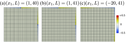
Figure 3: The plot of $\Delta_{\bm{R}}$ in Eq. (37) for the three settings of $(x_{1},L)$. In the panel (a), the two plaquettes at $\bm{R}=(L,L/2)$ and $(L/2,L)$ produce the irrational contribution in Table 2.

To pin down the origin of the mismatch, we compare $(\hat{U}_{xy}^{\text{(a)}})_{\bm{R},\bm{R}}$ and $(\hat{U}_{xy}^{\text{(b)}})_{\bm{R},\bm{R}}$ by plotting

$$\Delta_{\bm{R}}\equiv\frac{1}{2\pi}\text{Im}\ln\frac{(\hat{U}_{xy}^{\text{(a)}})_{\bm{R},\bm{R}}}{(\hat{U}_{xy}^{\text{(b)}})_{\bm{R},\bm{R}}}\mod 1$$ (37)

as a function of $\bm{R}$. Figure 3 shows that the discrepancy originates purely from the boundary. In fact, the sum of $\Delta_{\bm{R}}$ over the boundary (i.e. $R_{x}=x_{L}$ or $R_{y}=y_{L}$) precisely accounts for the difference $\Delta\tilde{q}_{xy}^{\text{(a)}}-\Delta\tilde{q}_{xy}^{\text{(b)}}$. Furthermore, $(\hat{U}_{xy})_{\bm{R},\bm{R}}^{\text{(b)}}$ for the plaquettes near the boundary has a small amplitude and $|\langle\Phi_{0}|\hat{U}_{xy}|\Phi_{0}\rangle|$ decays exponentially with the system size ($e^{-cL}$ with $c\simeq 1.5$ in this particular model). These issues are the manifestation of the violation of the periodicity discussed in Sec. II.1.

C.2 Model 2

The second model is the orthogonal stacking of Su-Schrieffer-Heeger chains (Fig. 4). The tight-binding Hamiltonian reads

$$H_{\bm{k}}= -\begin{pmatrix}0&0&e^{ik_{x}}&0\\ 0&0&0&e^{ik_{y}}\\ e^{-ik_{x}}&0&0&0\\ 0&e^{-ik_{y}}&0&0\\ \end{pmatrix}.$$ (38)

This time we have two occupied bands and we place two ions at every lattice site:

$$\tilde{q}_{xy,\text{ions}}{{}^{\prime}} =2\tilde{q}_{xy,\text{ions}}=\frac{(2x_{1}+L-1)^{2}}{2}.$$ (39)

We analyze this model in the same way as in Appendix B and find $\Delta\tilde{q}_{xy}^{\text{(a)}}{{}^{\prime}}=\tilde{q}_{xy}^{\text{(a)}}{{}^{\prime}}-\tilde{q}_{xy,\text{ions}}{{}^{\prime}}$. For the atomic limit of this insulator where an electron is localized at both $\bm{x}=\bm{R}+(\frac{1}{2},0)$ and $\bm{R}+(0,\frac{1}{2})$ for every unit cell, we find

$$(\hat{U}_{xy}^{\text{(b)}}{{}^{\prime}})_{\bm{R},\bm{R}}=e^{2\pi i[R_{x}(R_{y}+1/2)+(R_{x}+1/2)R_{y}]/L^{2}},$$ (40)

$$\tilde{q}_{xy}^{\text{(b)}}{{}^{\prime}}=\frac{1}{2\pi}\sum_{\bm{R}}\text{Im}\ln(\hat{U}_{xy}^{\text{(b)}}{{}^{\prime}})_{\bm{R},\bm{R}}=\frac{(2x_{1}+L-1)(2x_{1}+L)}{2}.$$ (41)

We list $\Delta\tilde{q}_{xy}^{\text{(b)}}{{}^{\prime}}=\tilde{q}_{xy}^{\text{(b)}}{{}^{\prime}}-\tilde{q}_{xy,\text{ions}}{{}^{\prime}}$ in Table 3. Although we do not expect any quadrupole moment in this model, we found $\Delta\tilde{q}_{xy}=1/2$ mod 1 for the case (b) when $x_{1}=1$ and $L$ is even.

Table 3: Analytic expression of $\Delta\tilde{q}_{xy}$ for the second model in the limit of large $L$.

$(x_{1},L)$	$(1,\text{even})$	$(1,\text{odd})$	$(-\frac{L-1}{2},\text{odd})$
$\Delta\tilde{q}_{xy}^{\text{(a)}}{{}^{\prime}}$	$0$	$0$	$0$
$\Delta\tilde{q}_{xy}^{\text{(b)}}{{}^{\prime}}$	$\frac{1}{2}$	$0$	$0$

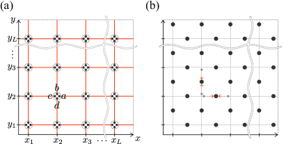
Figure 4: Illustration of the second model (a) and the atomic limit (b).

C.3 Stacking of the two models

Band insulators considered in Appendices C.1 and C.2 possesse a nonzero bulk polarization. We can fix it by stacking them together. We show the values of $\Delta\tilde{q}_{xy}$ in the large $L$ limit in Table 4. As we can see, problems of $\tilde{q}_{xy}$ still persist in the absence of the bulk polarization.

Table 4: The analytic expression of $\Delta\tilde{q}_{xy}$ for the stacked model in the limit of large $L$.

$(x_{1},L)$	$(1,\text{even})$	$(1,\text{odd})$	$(-\frac{L-1}{2},\text{odd})$
$\Delta\tilde{q}_{xy}^{\text{(a)}}+\Delta\tilde{q}_{xy}^{\text{(a)}}{{}^{\prime}}$	$\frac{1}{4}+\frac{1}{\pi}\arctan\frac{2}{\pi}$	$\frac{3}{4}$	$0$
$\Delta\tilde{q}_{xy}^{\text{(b)}}+\Delta\tilde{q}_{xy}^{\text{(b)}}{{}^{\prime}}$	$\frac{1}{4}$	$\frac{1}{4}$	$\frac{1}{4}$

Let us summarize what we learned about $\tilde{q}_{xy}$ through these examples: (i) $\Delta\tilde{q}_{xy}=\tilde{q}_{xy}-\tilde{q}_{xy,\text{ions}}$ depends on $x_{1}$ and the parity of $L$; (ii) it is not always quantized even under the $C_{4}$ symmetry; and (iii) it takes different values for two states (a) and (b) in the same phase (i.e., adiabatically connected).

References

- Parameswaran and Wan (2017) S. A. Parameswaran and Y. Wan, Physics 10, 132 (2017).
- Schindler et al. (2018) F. Schindler, A. M. Cook, M. G. Vergniory, Z. Wang, S. S. P. Parkin, B. A. Bernevig, and T. Neupert, Sci. Adv. 4, eaat0346 (2018).
- Peng et al. (2017) Y. Peng, Y. Bao, and F. von Oppen, Phys. Rev. B 95, 235143 (2017).
- Langbehn et al. (2017) J. Langbehn, Y. Peng, L. Trifunovic, F. von Oppen, and P. W. Brouwer, Phys. Rev. Lett. 119, 246401 (2017).
- Song et al. (2017) Z. Song, Z. Fang, and C. Fang, Phys. Rev. Lett. 119, 246402 (2017).
- Benalcazar et al. (2017a) W. A. Benalcazar, B. A. Bernevig, and T. L. Hughes, Science 357, 61 (2017a).
- Benalcazar et al. (2017b) W. A. Benalcazar, B. A. Bernevig, and T. L. Hughes, Phys. Rev. B 96, 245115 (2017b).
- Fang and Fu (2017) C. Fang and L. Fu, arXiv:1709.01929 (2017).
- Ezawa (2018) M. Ezawa, Phys. Rev. Lett. 120, 026801 (2018).
- Shapourian et al. (2018) H. Shapourian, Y. Wang, and S. Ryu, Phys. Rev. B 97, 094508 (2018).
- Zhu (2018) X. Zhu, Phys. Rev. B 97, 205134 (2018).
- Yan et al. (2018) Z. Yan, F. Song, and Z. Wang, Phys. Rev. Lett. 121, 096803 (2018).
- Wang et al. (2018a) Y. Wang, M. Lin, and T. L. Hughes, ArXiv e-prints (2018a), arXiv:1804.01531 [cond-mat.supr-con] .
- Wang et al. (2018b) Q. Wang, C.-C. Liu, Y.-M. Lu, and F. Zhang, ArXiv e-prints (2018b), arXiv:1804.04711 [cond-mat.mes-hall] .
- Khalaf et al. (2018) E. Khalaf, H. C. Po, A. Vishwanath, and H. Watanabe, Phys. Rev. X 8, 031070 (2018).
- Khalaf (2018) E. Khalaf, Phys. Rev. B 97, 205136 (2018).
- Trifunovic and Brouwer (2019) L. Trifunovic and P. W. Brouwer, Phys. Rev. X 9, 011012 (2019).
- Okuma et al. (2018) N. Okuma, M. Sato, and K. Shiozaki, arXiv e-prints , arXiv:1810.12601 (2018), arXiv:1810.12601 [cond-mat.mes-hall] .
- Resta and Vanderbilt (2007) R. Resta and D. Vanderbilt, “Theory of polarization: A modern approach,” in Physics of Ferroelectrics: A Modern Perspective (Springer Berlin Heidelberg, Berlin, Heidelberg, 2007) pp. 31–68.
- Lines and Glass (2001) M. E. Lines and A. M. Glass, Principles and Applications of Ferroelectrics and Related Materials (Oxford University Press, 2001).
- Kittel (2004) C. Kittel, Introduction to Solid State Physics (Wiley, 2004).
- Martin (1974) R. M. Martin, Phys. Rev. B 9, 1998 (1974).
- Aligia and Ortiz (1999) A. A. Aligia and G. Ortiz, Phys. Rev. Lett. 82, 2560 (1999).
- Vanderbilt and King-Smith (1993) D. Vanderbilt and R. D. King-Smith, Phys. Rev. B 48, 4442 (1993).
- King-Smith and Vanderbilt (1993) R. D. King-Smith and D. Vanderbilt, Phys. Rev. B 47, 1651 (1993).
- Ortiz and Martin (1994) G. Ortiz and R. M. Martin, Phys. Rev. B 49, 14202 (1994).
- Souza et al. (2000) I. Souza, T. Wilkens, and R. M. Martin, Phys. Rev. B 62, 1666 (2000).
- Watanabe and Oshikawa (2018) H. Watanabe and M. Oshikawa, Phys. Rev. X 8, 021065 (2018).
- Resta (1998) R. Resta, Phys. Rev. Lett. 80, 1800 (1998).
- Trifunovic et al. (2019) L. Trifunovic, S. Ono, and H. Watanabe, Phys. Rev. B 100, 054408 (2019).
- Wheeler et al. (2018) W. A. Wheeler, L. K. Wagner, and T. L. Hughes, (2018), arXiv:1812.06990 .
- Kang et al. (2018) B. Kang, K. Shiozaki, and G. Y. Cho, (2018), arXiv:1812.06999 .
- Note (1) We explain why this perturbation theory fails in Appendix A.
- Agarwala et al. (2019) A. Agarwala, V. Juricic, and B. Roy, arXiv e-prints , arXiv:1902.00507 (2019), arXiv:1902.00507 [cond-mat.mes-hall] .
- Lin et al. (2019) Z.-K. Lin, H.-X. Wang, M.-H. Lu, and J.-H. Jiang, arXiv e-prints , arXiv:1903.05997 (2019), arXiv:1903.05997 [cond-mat.str-el] .
- Benalcazar et al. (2019) W. A. Benalcazar, T. Li, and T. L. Hughes, Phys. Rev. B 99, 245151 (2019).
- Note (2) See also Appendix of Ref. \rev@citealpnumKen where the dependence of is discussed using a tight-binding model.
- Marzari and Vanderbilt (1997) N. Marzari and D. Vanderbilt, Phys. Rev. B 56, 12847 (1997).
- Resta and Sorella (1999) R. Resta and S. Sorella, Phys. Rev. Lett. 82, 370 (1999).
- Note (3) Even when , Eq. (23\@@italiccorr) is still violated because the exponent of Eq. (26\@@italiccorr) is , not .