Cell-Free Millimeter-Wave Massive MIMO Systems with Limited Fronthaul Capacity

Abstract

Network densification, massive multiple-input multiple-output (MIMO) and millimeter-wave (mmWave) bands have recently emerged as some of the physical layer enablers for the future generations of wireless communication networks (5G and beyond). Grounded on prior work on sub-6 GHz cell-free massive MIMO architectures, a novel framework for cell-free mmWave massive MIMO systems is introduced that considers the use of low-complexity hybrid precoders/decoders while factors in the impact of using capacity-constrained fronthaul links. A suboptimal pilot allocation strategy is proposed that is grounded on the idea of clustering by dissimilarity. Furthermore, based on mathematically tractable expressions for the per-user achievable rates and the fronthaul capacity consumption, max-min power allocation and fronthaul quantization optimization algorithms are proposed that, combining the use of block coordinate descent methods with sequential linear optimization programs, ensure a uniformly good quality of service over the whole coverage area of the network. Simulation results show that the proposed pilot allocation strategy eludes the computational burden of the optimal small-scale CSI-based scheme while clearly outperforming the classical random pilot allocation approaches. Moreover, they also reveal the various existing trade-offs among the achievable max-min per-user rate, the fronthaul requirements and the optimal hardware complexity (i.e., number of antennas, number of RF chains).

I Introduction

I-A Motivation and previous work

Driven by the continuously increasing demands for high system throughput, low latency, ultra reliability, improved fairness and near-instant connectivity, fifth generation (5G) wireless communication networks are being standardized [1] while, at the same time, insights and innovations from industry and academia are paving the road for the coming of the sixth generation (6G) [2]. As stated by Marzetta et al. in [3, Chapter 1], there are three basic pillars at the physical layer that can be used to sustain the spectral and energy efficiencies that these networks are expected to provide: (i) employing massive multiple-input multiple-output (MIMO), (ii) using ultra dense network (UDN) deployments, and (iii) exploiting new frequency bands.

Massive MIMO systems, equipped with a large number of antenna elements, are intended to be used as multiuser-MIMO (MU-MIMO) arrangements in which the number of antenna elements at each access point (AP) is much larger than the number of mobile stations (MSs) simultaneously served over the same time/frequency resources. The operation of massive MIMO schemes is based on the availability of channel state information (CSI) acquired through time division duplexing (TDD) operation and the use of uplink (UL) pilot signals. Such a setting allows for very high spectral and energy efficiencies using simple linear signal processing in the form of conjugate beamforming or zero-forcing (ZF) [4, 3].

In UDNs, a large number of APs deployed within a given coverage area cooperate to jointly transmit/receive to/from a (relatively) reduced number of MSs thanks to the availability of high-performance low-latency fronthaul links connecting the APs to a central coordinating node. Coordination among APs can effectively control (or even eliminate) intercellular interference in an approach that was first referred to as network MIMO [5, 6], later led to the concept of coordinated multipoint (CoMP) transmission [7] and, more recently, to that of cloud radio access network (C-RAN) [8]. In a C-RAN, the APs, which are treated as a distributed MIMO system, are connected to a cloud-computing based central processing unit (CPU) in charge, among many others, of the baseband processing tasks of all APs. Conceptually similar to the C-RAN architecture, but explicitly relying on assumptions specific of the massive MIMO regime, distributed massive MIMO-based UDNs have been recently termed as cell-free massive MIMO networks [9, 10]. In these networks, a massive number of APs connected to a CPU are distributed across the coverage area and, as in the cellular collocated massive MIMO schemes, exploit the channel hardening and favorable propagation properties to coherently serve a large number of MSs over the same time/frequency resources. Typically using simple linear signal processing schemes, they are claimed to provide uniformly good quality of service (QoS) to the whole set of served MSs irrespective of their particular location in the coverage area.

Since the microwave radio spectrum (from 300 MHz to 6 GHz) is highly congested, the use of massive antenna systems and network densification alone may not be sufficient to meet the QoS demands in next generation wireless communications networks. Thus, another promising physical layer solution that is expected to play a pivotal role in 5G and beyond 5G communication systems is to increase the available spectrum by exploring new less-congested frequency bands. In particular, there has been a growing interest in exploiting the so-called millimeter wave (mmWave) bands [11, 12, 13, 14]. The available spectrum at these frequencies is orders of magnitude higher than that available at the microwave bands and, moreover, the very small wavelengths of mmWaves, combined with the technological advances in low-power CMOS radio frequency (RF) miniaturization, allow for the integration of a large number of antenna elements into small form factors. Large antenna arrays can then be used to effectively implement mmWave massive MIMO schemes (see, for instance, [15, 16] and references therein) that, with appropriate beamforming, can more than compensate for the orders-of-magnitude increase in free-space path-loss produced by the use of higher frequencies.

The performance of cell-free massive MIMO using conventional sub-6 GHz frequency bands and assuming infinite-capacity fronthaul links has been extensively studied in, for instance, [10, 17, 18, 19]. Cell-free massive MIMO networks using capacity-constrained fronthaul links have also been considered in [20, 21] but assuming, again, the use of fully digital precoders in conventional sub-6 GHz frequency bands. Sub-6 GHz massive MIMO systems are often assumed to implement a fully-digital baseband signal processing requiring a dedicated RF chain for each antenna element. The present status of mmWave technology, however, characterized by high-power consumption levels and high production costs, precludes the fully-digital implementation of massive MIMO architectures, and typically forces mmWave systems to rely on hybrid digital-analog signal processing architectures. In these hybrid transceiver architectures, a large antenna array connects to a limited number of RF chains via high-dimensional RF precoders, typically implemented using analog phase shifters and/or analog switches, and low-dimensional baseband digital precoders are then used at the output of the RF chains [22, 23, 24]. The network of phase shifters connecting the array of antennas to the RF chains determines whether the structure is fully or partially connected [25]. Thus, the assumptions, methods and analytical expressions in [10, 17, 18, 19, 20, 21] cannot by applied directly when assuming the use of mmWave frequency bands. Despite its evident potential, as far as we know, besides [26, 27] there is no other research work on cell-free mmWave massive MIMO systems and, furthermore, the authors of these works did not face one of the main challenges in the implementation of cooperative UDNs, that is, the fact that these systems require of a substantial information exchange between the APs and the CPU via capacity-constrained fronthaul links. Moreover, they also considered the use of oversimplified mmWave channel models and RF precoding stages, without constraining the available number of RF-chains at each AP.

I-B Aim and contributions

Motivated by the above considerations, our main aim in this paper is to address the design and performance evaluation of realistic cell-free mmWave massive MIMO systems using hybrid precoders and assuming the availability of capacity-constrained fronthaul links connecting the APs and the CPU. The main contributions of our work can be summarized as follows:

• The performance of both the downlink (DL) and UL of cell-free mmWave massive MIMO systems is considered with particular emphasis on the per-user rate, rather than the system sum-rate, by posing max-min fairness resource allocation problems that take into account the effects of imperfect channel estimation, power control, non-orthogonality of pilot sequences, and fronthaul capacity constraints. Instead of assuming the use of rather simple uniform quantization processes when forwarding information on the capacity-constrained fronthauls, the proposed optimization problems assume the use of large-block lattice quantization codes able to approximate a Gaussian quantization noise distribution. Optimal solutions to these problems are proposed that combine the use of block coordinate descent methods with sequential linear programs.

• A hybrid beamforming implementation is proposed where the RF high-dimensionality phase shifter-based precoding/decoding stage is based on large-scale second-order statistics of the propagation channel, and hence does not need the estimation of high-dimensionality instantaneous CSI. The low-dimensionality baseband MU-MIMO precoding/decoding stage can then be easily implemented by standard signal processing schemes using small-scale estimated CSI. As will be shown in the numerical results section, such a reduced complexity hybrid precoding scheme, when combined with appropriate user selection, performs very well in the fronthaul capacity-constrained UDN mmWave-based scenarios under consideration.

• A suboptimal pilot allocation strategy is proposed that, based on the idea of clustering by dissimilarity, avoids the computational complexity of the optimal pilot allocation scheme. The performance of the proposed dissimilarity cluster-based pilot assignment algorithm is compared with that of both the pure random pilot allocation approach and the balanced random pilot strategy.

• For those cases in which the number of active MSs in the network is greater than the number of available RF chains at a particular AP, a MS selection algorithm is proposed that aims at maximizing the minimum average sum-energy (i.e., Frobenius norm) of the equivalent channel between the APs and any of the active MSs, constrained by the fact that each AP can only beamform to a number of MSs less or equal than the number of available RF chains.

I-C Paper organization and notational remarks

The remainder of this paper is organized as follows. In Section II the proposed cell-free mmWave massive MIMO system is introduced. Different subsections are devoted to the description of the channel model, the large-scale and small-scale training phases, the channel estimation process, and the DL and UL payload transmission phases. The achievable DL and UL rates are presented in Section III and further developed in Appendices A and B. Section IV is dedicated to the calculation of the capacity consumption of both the DL and UL fronthaul links. The pilot assignment, power allocation and quantization optimization processes are described in Sections V and VI. Numerical results and discussions are provided in Section VII and, finally, concluding remarks are summarized in Section VIII.

Notation: Vectors and matrices are denoted by lower-case and upper-case boldface symbols. The $q$-dimensional identity matrix is represented by $\boldsymbol{I}_{q}$. The operator $\det(\boldsymbol{X})$ represents the determinant of matrix $\boldsymbol{X}$, $\operatorname{tr}(\boldsymbol{X})$ denotes its trace, $\|\boldsymbol{X}\|_{F}$ is its Frobenius norm, whereas $\boldsymbol{X}^{-1}$, $\boldsymbol{X}^{T}$, $\boldsymbol{X}^{*}$ and $\boldsymbol{X}^{H}$ denote its inverse, transpose, conjugate and conjugate transpose (also known as Hermitian), respectively. With a slight abuse of notation, the operator $\operatorname{diag}(\boldsymbol{x})$ is used to denote a diagonal matrix with the entries of vector $\boldsymbol{x}$ on its main diagonal, and the operator $\operatorname{diag}(\boldsymbol{X})$ is used to denote a vector containing the entries in the main diagonal of matrix $\boldsymbol{X}$. The expectation operator is denoted by $\mathbb{E}\{\cdot\}$. Finally, $\mathcal{CN}(\boldsymbol{m},\boldsymbol{R})$ denotes a circularly symmetric complex Gaussian vector distributions with mean $\boldsymbol{m}$ and covariance $\boldsymbol{R}$, $\mathcal{N}(0,\sigma^{2})$ denotes a real valued zero-mean Gaussian random variable with standard deviation $\sigma$, and $\mathcal{U}[a,b]$ represents a random variable uniformly distributed in the range $[a,b]$.

II System model

Let us consider a cell-free massive MIMO system where a CPU coordinates the communication between $M$ APs and $K$ single-antenna MSs randomly distributed in a large area. Each of the APs communicates with the CPU via error-free fronthaul links with DL and UL capacities ${C_{F}}_{d}$ and ${C_{F}}_{u}$, respectively. Baseband processing of the transmitted/received signals is performed at the CPU, while the RF operations are carried out at the APs. Each AP is equipped with an array of $N>K$ antennas and $L\leq N$ RF chains. A fully-connected architecture is considered where each RF chain is connected to the whole set of antenna elements using $N$ analog phase shifters. Without loss of essential generality, it is assumed in this paper that the number of active RF chains at each of the APs in the network is equal to $L_{A}=\min\{K,L\}$. That is, if $K\leq L$, all APs in the cell-free network provide service to the whole set of MSs and if $K>L$, instead, each AP can only provide service to $L$ out of the $K$ MSs in the network and, thus, an algorithm must be devised to decide which are the MSs to be beamformed by each of the APs.

Figure 1: Allocation of the samples in large-scale and short-scale coherence intervals.

The propagation channels linking the APs to the MSs are typically characterized by small-scale parameters that are (almost) static over a coherence time-frequency interval of $\tau_{c}$ time-frequency samples (see [3, Chapter 2]), and large-scale parameters (i.e., path loss propagation losses and covariance matrices) that can be safely assumed to be static over a time-frequency interval ${\tau_{L}}_{c}\gg\tau_{c}$. As shown in the following subsections, these channel characteristics can be leveraged to simplify both the channel estimation and the precoding/combining processes. In particular, DL and UL transmissions between APs and MSs are organized in a half-duplex TDD operation whereby each coherence interval is split into three phases, namely, the UL training phase, the DL payload data transmission phase and the UL payload data transmission phase, and every large-scale coherence interval ${\tau_{L}}_{c}$ the system performs an estimation of the large-scale parameters of the channel (see Fig. 1). In the UL training phase, all MSs transmit UL training orthogonal pilots allowing the APs to estimate the propagation channels to every MS in the network. Subsequently, these channel estimates are used to detect the signals transmitted from the MSs in the UL payload data transmission phase and to compute the precoding filters governing the DL payload data transmission. Not shown are guard intervals between UL and DL transmissions.

II-A Channel Model

MmWave propagation is characterized by very high distance-based propagation losses that lead to sparse scattering multipath propagation. Furthermore, the use of mmWave transmitters and receivers with large tightly-packet antenna arrays results in high antenna correlation levels. These characteristics make most of the statistical channel models used in conventional sub-6 GHz MIMO research work inaccurate when dealing with mmWave scenarios. Thus, a modified version of the discrete-time narrowband clustered channel model proposed by Akdeniz et al. in [13] and further extended by Samimi and Rappaport in [28] will be used in this paper to capture the peculiarities of mmWave channels.

The link between the $m$th AP and the $k$th MS will be considered to be in one out of three possible conditions: outage, line-of-sight (LOS) or non-line-of-sight (NLOS) with probabilities:

$$p_{out}(d_{mk})=\max\left(0,1-e^{-a_{out}d_{mk}+b_{out}}\right),$$ (1a)

$$p_{\lx@glossaries@gls@link{acronym}{LOS}{\leavevmode LOS}}(d_{mk})=\left(1-p_{out}(d_{mk})\right)e^{-a_{\lx@glossaries@gls@link{acronym}{LOS}{\leavevmode LOS}}d_{mk}},$$ (1b)

$$p_{\lx@glossaries@gls@link{acronym}{NLOS}{\leavevmode NLOS}}(d_{mk})=1-p_{out}(d_{mk})-p_{\lx@glossaries@gls@link{acronym}{LOS}{\leavevmode LOS}}(d_{mk}),$$ (1c)

respectively, where $d_{mk}$ is the distance (in meters) between the AP and the MS, and, according to [13, Table I], $1/a_{out}=30$ m, $b_{out}=5.2$, and $1/a_{\lx@glossaries@gls@link{acronym}{LOS}{\leavevmode LOS}}=67.1$ m. Those links that are in outage will be characterized with infinite propagation losses, while for the links that are not in outage, the propagation losses will be characterized using a standard linear model with shadowing as

$$\operatorname{PL}(d_{mk})[dB]=\alpha+10\beta\log_{10}(d_{mk})+\chi_{mk},$$ (2)

where $\alpha$ and $\beta$ are the least square fits of floating intercept and slope and depend on the carrier frequency and on whether the link is in LOS or NLOS (see [13, Table I]), and $\chi_{mk}$ denotes the large-scale shadow fading component, which is modelled as a zero mean spatially correlated normal random variable with standard deviation $\sigma_{\chi}$ (again, see [13, Table I] to obtain the typical values of $\sigma_{\chi}$ for LOS and NLOS links) whose spatial correlation model is described in [10, (54)-(55)].

The UL channel vector $\boldsymbol{h}_{mk}\in\mathbb{C}^{N\times 1}$ between MS $k$ and AP $m$ will be modelled as the sum of the contributions of $C_{mk}$ scattering clusters, each contributing $P_{mk}$ propagation paths as

$$\boldsymbol{h}_{mk}=\sum_{c=1}^{C_{mk}}\sum_{p=1}^{P_{mk}}\alpha_{mk,cp}\boldsymbol{a}\left(\theta_{mk,cp},\phi_{mk,cp}\right),$$ (3)

where $\alpha_{mk,cp}$ is the complex small-scale fading gain on the $p$th path of cluster $c$, and $\boldsymbol{a}\left(\theta_{mk,cp},\phi_{mk,cp}\right)$ represents the AP normalized array response vector at the azimuth and elevation angles $\theta_{mk,cp}$ and $\phi_{mk,cp}$, respectively. These angles, as stated by Akdeniz et al. in [13, Section III.E] can be generated as wrapped Gaussians around the cluster central angles with standard deviation given by the root mean square (rms) angular spreads for the cluster. The azimuth cluster central angles are uniformly distributed in the range $[-\pi,\pi]$ and the elevation cluster central angles are set to the LOS elevation angle. Moreover, the cluster rms angular spreads are exponentially distributed with a mean equal to $1/\lambda_{\lx@glossaries@gls@link{acronym}{rms}{\leavevmode rms}}$ that depends on the carrier frequency and on whether we are considering the azimuth or elevation directions (see [13, Table I]). The number of clusters is distributed as a random variable of the form

$$C_{mk}\sim\max\left\{\text{Poisson}(\sigma_{C}),1\right\},$$ (4)

where $\sigma_{C}$ is set to the empirical mean of $C_{mk}$. The small-scale fading gains are distributed as

$$\alpha_{mk,cp}\sim\mathcal{CN}\left(0,\gamma_{mk,c}10^{-\operatorname{PL}(d_{mk})/10}\right),$$ (5)

where the cluster $c$ is assumed to contribute with a fraction of power given by

$$\gamma_{mk,c}=\frac{N\gamma^{\prime}_{mk,c}}{P_{mk}\sum_{j=1}^{C_{mk}}\gamma^{\prime}_{mk,j}},$$ (6)

with

$$\gamma^{\prime}_{mk,j}=U_{mk,j}^{r_{\tau}-1}10^{Z_{mk,j}/10},$$ (7)

$U_{mk,j}\sim\mathcal{U}[0,1]$, $Z_{mk,j}\sim\mathcal{N}(0,\zeta^{2})$, and the constants $r_{\tau}$ and $\zeta^{2}$ being treated as model parameters (see [13, Table I]).

Although the small-scale fading gains $\alpha_{mk,cp}$ are assumed to be static throughout the coherence interval and then change independently (i.e., block fading), the spatial covariance matrices

$$\begin{split}\boldsymbol{R}_{mk}=&\mathbb{E}\left\{\boldsymbol{h}_{mk}\boldsymbol{h}_{mk}^{H}\right\}\\ =&10^{-\operatorname{PL}(d_{mk})/10}\sum_{c=1}^{C_{mk}}\gamma_{mk,c}\\ &\times\sum_{p=1}^{P_{mk}}\boldsymbol{a}\left(\theta_{mk,cp},\phi_{mk,cp}\right)\boldsymbol{a}^{H}\left(\theta_{mk,cp},\phi_{mk,cp}\right),\end{split}$$ (8)

are assumed to vary at a much smaller pace (i.e., ${\tau_{L}}_{c}\gg\tau_{c}$).

II-B Large-scale training phase

II-B1 RF precoder/combiner design

In order to exploit the UL/DL channel reciprocity using the TDD frame structure shown in Fig. 1, it is assumed in this paper that the $N\times L_{A}$ RF matrix $\boldsymbol{W}_{m}^{RF}$, describing the effects of the active analog phase shifters at the $m$th AP, is common to the DL (RF precoding phase) and UL (RF combining phase). Furthermore, denoting by $\mathcal{K}_{m}=\left\{\kappa_{m1},\ldots,\kappa_{mL_{A}}\right\}$ the set of $L_{A}$ MSs beamformed by the $m$th AP, it is assumed that $\boldsymbol{W}_{m}^{RF}$ is a function of only the spatial channel covariance matrices $\left\{\boldsymbol{R}_{mk}\right\}_{k\in\mathcal{K}_{m}}$, known at the $m$th AP through spatial channel covariance estimation for hybrid analog-digital MIMO precoding architectures (see e.g. [29, 30, 31, 32]).

Using eigen-decomposition, the covariance matrix of the propagation channel linking MS k and AP $m$ can be expressed as $\boldsymbol{R}_{mk}=\boldsymbol{U}_{mk}\boldsymbol{\Lambda}_{mk}\boldsymbol{U}_{mk}^{H}$, where $\boldsymbol{\Lambda}_{mk}=\operatorname{diag}\left(\left[\lambda_{mk,1}\,\ldots\,\lambda_{mk,r_{mk}}\right]\right)$ contains the $r_{mk}$ non-null eigenvalues of $\boldsymbol{R}_{mk}$, and $\boldsymbol{U}_{mk}$ is the $N\times r_{mk}$ matrix of the corresponding eigenvectors. Hence, assuming the use of (constrained) statistical eigen beamforming [33, 34], the analog RF precoder/combiner can be designed as

$$\begin{split}\boldsymbol{W}_{m}^{RF}=&\begin{bmatrix}\boldsymbol{w}_{m\kappa_{m1}}^{RF}&\ldots&\boldsymbol{w}_{m\kappa_{mL_{A}}}^{RF}\end{bmatrix}\\ =&\begin{bmatrix}e^{-j\angle\boldsymbol{u}_{m\kappa_{m1},\max}}&\ldots&e^{-j\angle\boldsymbol{u}_{m\kappa_{mL_{A}},\max}}\end{bmatrix},\end{split}$$ (9)

where $\boldsymbol{u}_{mk,\max}$ is the dominant eigenvector of $\boldsymbol{R}_{mk}$ associated to the maximum eigenvalue $\lambda_{mk,\max}$, and the function $\angle\boldsymbol{x}$ returns the phase angles, in radians, for each element of the complex vector $\boldsymbol{x}$. Note that using the RF precoding/combining matrix, the equivalent channel vector between MS k and AP $m$, including the RF precoding/decoding matrix, is defined as

$$\boldsymbol{g}_{mk}={\boldsymbol{W}_{m}^{RF}}^{T}\boldsymbol{h}_{mk}\ \in\ \mathbb{C}^{L_{A}\times 1},$$ (10)

whose dimension is much less than the number of antennas of the massive MIMO array used at the $m$th AP, thus largely simplifying the small-scale training phase.

II-B2 Selection of MSs to beamform from each AP

As previously stated, in those highly probable cases in which the number of active MSs in the network is greater than the number of available RF chains at each AP (i.e., $K>L$), the $m$th AP, with $m\in\{1,\ldots,M\}$, can only beamform to a group of $L$ out of the $K$ MSs in the network, which are indexed by the set $\mathcal{K}_{m}=\left\{\kappa_{m1},\ldots,\kappa_{mL}\right\}$. As the RF beamforming matrices at the APs are a function of only the large-scale spatial channel covariance matrices and are common to both the UL and the DL, the selection of the sets of MSs to beamform from each AP must also be based only on the available large-scale CSI. Inspired by the Frobenius norm-based suboptimal user selection algorithm proposed by Shen et al. in [35], a selection algorithm is proposed that aims at maximizing the sum of the average energy (i.e., average Frobenius norm) of the equivalent channels (including the corresponding beamformer) between the $M$ APs and the $K$ MSs with the constraints that, first, the minimum average energy of the equivalent channel between the $M$ APs and any of the active MSs must be maximized and, second, that each AP can only beamform to $L$ MSs. Note that this optimization problem, which tends to provide some degree of (average) max-min fairness among MSs, can be efficiently solved by using an iterative reverse-delete algorithm (similar to that used in graph theory to obtain a minimum spanning tree from a given connected, edge-weighted graph). In particular, at the beginning of the $i$th iteration of the algorithm the cell-free network is represented by a very simple edge-weighted directed graph with $M$ source nodes and $K$ sink nodes, where the $m$th source node, representing the $m$th AP, is connected to a group $\mathcal{K}_{m}^{(i)}$ of sink nodes, representing the active MSs beamformed by the $m$th AP. The connection (edge) between the $m$th source node and the $l$th sink node in $\mathcal{K}_{m}^{(i)}$ is weighted by the average Frobenius norm of the equivalent channel linking the $m$th AP and MS $l\in\mathcal{K}_{m}^{(i)}$, that can be obtained as

$$\xi_{ml}=\mathbb{E}\left\{\left\|{\boldsymbol{w}_{ml}^{RF}}^{T}\boldsymbol{h}_{ml}\right\|_{F}^{2}\right\}={\boldsymbol{w}_{ml}^{RF}}^{T}\boldsymbol{R}_{ml}\boldsymbol{w}_{ml}^{RF}.$$ (11)

The average sum energy of the equivalent channels between the $M$ APs and MS $k$ at the beginning of the $i$th iteration is

$$\mathcal{E}_{k}^{(i)}=\sum_{m\in\mathcal{M}_{k}^{(i)}}\xi_{mk},$$ (12)

where $\mathcal{M}_{k}^{(i)}$ is the set of APs beamforming to MS $k$ at the beginning of the $i$th iteration. During this iteration, the reverse-delete algorithm removes the edge (i.e., the RF chain and associated beamformer) that, first, goes out of one of those APs still beamforming to more than $L$ MSs and, second, has the minimum weight maximizing the minimum average sum energy after removal. The algorithm begins with a fully connected graph and stops when all APs beamform to exactly $L$ MSs. Hence, note that $M(K-L)$ iterations are needed to select the sets $\mathcal{K}_{m}$ for $m\in\{1,\ldots,M\}$.

II-C Small-scale training phase

Communication in any coherence interval of a TDD-based massive MIMO system invariably starts with the MSs sending the pilot sequences to allow the channel to be estimated at the APs. Let $\tau_{p}$ denote the UL training phase duration (measured in samples on a time-frequency grid) per coherence interval. During the UL training phase, all $K$ MSs simultaneously transmit pilot sequences of $\tau_{p}$ samples to the APs and thus, the $L_{A}\times\tau_{p}$ received UL signal matrix at the $m$th AP is given by

$${\boldsymbol{Y}_{p}}_{m}=\sqrt{\tau_{p}P_{p}}\sum_{k^{\prime}=1}^{K}\boldsymbol{g}_{mk^{\prime}}\boldsymbol{\varphi}_{k^{\prime}}^{T}+{\boldsymbol{N}_{p}}_{m},$$ (13)

where $P_{p}$ is the transmit power of each pilot symbol, $\boldsymbol{\varphi}_{k}$ denotes the $\tau_{p}\times 1$ training sequence assigned to MS $k$, with $\|\boldsymbol{\varphi}_{k}\|_{F}^{2}=1$, and ${\boldsymbol{N}_{p}}_{m}$ is an $L_{A}\times\tau_{p}$ matrix of i.i.d. additive noise samples with each entry distributed as $\mathcal{CN}(0,\sigma_{u}^{2}(N))$. Ideally, training sequences should be chosen to be mutually orthogonal, however, since in most practical scenarios it holds that $K>\tau_{p}$, a given training sequence is assigned to more than one MS, thus resulting in the so-called pilot contamination, a widely studied phenomenon in the context of collocated massive MIMO systems [36].

II-D Channel estimation

Channel estimation is known to play a central role in the performance of massive MIMO schemes [37] and also in the specific context of cell-free architectures [10]. The minimum mean square error (MMSE) estimation filter for the channel between the $k$th active MS and the $m$th AP can be calculated as

$$\begin{split}\boldsymbol{D}_{mk}&=\arg\min_{\boldsymbol{D}}\mathbb{E}\left\{\left\|\boldsymbol{g}_{mk}-\boldsymbol{D}{\boldsymbol{Y}_{p}}_{m}\boldsymbol{\varphi}_{k}^{*}\right\|^{2}\right\}\\ &=\sqrt{\tau_{p}P_{p}}\boldsymbol{R}_{mk}^{RF}\boldsymbol{Q}_{mk}^{-1},\end{split}$$ (14)

where

$$\boldsymbol{R}_{mk}^{RF}=\mathbb{E}\left\{\boldsymbol{g}_{mk}\boldsymbol{g}_{mk}^{H}\right\}={\boldsymbol{W}_{m}^{RF}}^{T}\boldsymbol{R}_{mk}{\boldsymbol{W}_{m}^{RF}}^{*},$$ (15)

and

$$\boldsymbol{Q}_{mk}=\tau_{p}P_{p}\sum_{k^{\prime}=1}^{K}\boldsymbol{R}_{mk^{\prime}}^{RF}\left|\boldsymbol{\varphi}_{k^{\prime}}^{T}\boldsymbol{\varphi}_{k}^{*}\right|^{2}+\sigma_{u}^{2}(N)\boldsymbol{I}_{L_{A}}.$$ (16)

Hence, the corresponding estimated channel vector can be expressed as

$$\hat{\boldsymbol{g}}_{mk}=\boldsymbol{D}_{mk}{\boldsymbol{Y}_{p}}_{m}\boldsymbol{\varphi}_{k}^{*}=\sqrt{\tau_{p}P_{p}}\boldsymbol{R}_{mk}^{RF}\boldsymbol{Q}_{mk}^{-1}{\boldsymbol{Y}_{p}}_{m}\boldsymbol{\varphi}_{k}^{*}.$$ (17)

The MMSE channel vector estimates can be shown to be distributed as ${\hat{\boldsymbol{g}}}_{mk}\sim\mathcal{CN}\left(\boldsymbol{0},{\hat{\boldsymbol{R}}}_{mk}^{RF}\right)$, where

$$\hat{\boldsymbol{R}}_{mk}^{RF}\triangleq\tau_{p}P_{p}\boldsymbol{R}_{mk}^{RF}\boldsymbol{Q}_{mk}^{-1}{\boldsymbol{R}_{mk}^{RF}}^{H}.$$ (18)

Furthermore, the channel vector $\boldsymbol{g}_{mk}$ can be decomposed as $\boldsymbol{g}_{mk}=\hat{\boldsymbol{g}}_{mk}+\tilde{\boldsymbol{g}}_{mk}$, where $\tilde{\boldsymbol{g}}_{mk}$ is the MMSE channel estimation error, which is statistically independent of both $\boldsymbol{g}_{mk}$ and $\hat{\boldsymbol{g}}_{mk}$.

II-E Downlink payload data transmission

Let us define $\boldsymbol{s}_{d}=\left[{s_{d}}_{1}\ldots{s_{d}}_{K}\right]^{T}$ as the $K\times 1$ vector of symbols jointly (cooperatively) transmitted from the APs to the MSs, such that $E\left\{\boldsymbol{s}_{d}\boldsymbol{s}_{d}^{H}\right\}=\boldsymbol{I}_{K}$. Let us also define $\boldsymbol{x}_{m}=\mathcal{P}_{m}\left(\boldsymbol{s}_{d}\right)$ as the $N\times 1$ vector of signals transmitted from the $m$th AP, where $\mathcal{P}_{m}\left(\boldsymbol{s}_{d}\right)$ is used to denote the mathematical operations (linear and/or non-linear) used to obtain $\boldsymbol{x}_{m}$ from $\boldsymbol{s}_{d}$. Note that this vector must comply with a power constraint $\mathbb{E}\left\{\left\|\boldsymbol{x}_{m}\right\|_{F}^{2}\right\}\leq\overline{P}_{m}$, where $\overline{P}_{m}$ is the maximum average transmit power available at AP $m$. Using this notation, the signal received by MS $k$ can be expressed as

$${y_{d}}_{k}=\sum_{m=1}^{M}\boldsymbol{h}_{mk}^{T}\boldsymbol{x}_{m}+{n_{d}}_{k},$$ (19)

where ${n_{d}}_{k}\sim\mathcal{CN}(0,\sigma_{d}^{2})$ is the Gaussian noise sample at MS $k$. The vector $\boldsymbol{y}_{d}=\left[{y_{d}}_{1}\,\ldots\,{y_{d}}_{K}\right]^{T}$ containing the signals received by the $K$ scheduled MSs in the network can then be expressed as

$$\boldsymbol{y}_{d}=\sum_{m=1}^{M}\boldsymbol{H}_{m}^{T}\boldsymbol{x}_{m}+\boldsymbol{n}_{d},$$ (20)

where $\boldsymbol{H}_{m}=\left[\boldsymbol{h}_{m1}\,\ldots\,\boldsymbol{h}_{mK}\right]$ and $\boldsymbol{n}_{d}=\left[{n_{d}}_{1}\,\ldots\,{n_{d}}_{K}\right]^{T}$.

The mathematical operations that symbol vector $\boldsymbol{s}_{d}$ undergoes before being transmitted, generically represented as $\boldsymbol{x}_{m}=\mathcal{P}_{m}(\boldsymbol{s}_{d})$, for all $m\in\{1,\ldots,M\}$, include, first, a baseband precoding task at the CPU, second, a compressing process of all or part of the data that must be sent from the CPU to the APs through the fronthaul links and, third, an RF precoding task at each of the APs. Let us denote by ${\mathcal{Q}_{d}}_{m}(\boldsymbol{x})$ and ${\mathcal{Q}_{d}}_{m}^{-1}(\boldsymbol{x})$ the quantization and unquantization mathematical operations performed by the compress-after-precoding (CAP)-based CPU-AP functional split on a vector of signal samples $\boldsymbol{x}$ to be transmitted by the $m$th AP. Due to the distortion introduced by the quantization/unquantization processes, we have that [38, 39]

$$\hat{\mathcal{Q}}_{dm}(\boldsymbol{x})\triangleq{\mathcal{Q}_{d}}_{m}^{-1}({\mathcal{Q}_{d}}_{m}(\boldsymbol{x}))=\boldsymbol{x}+{\boldsymbol{q}_{d}}_{m},$$ (21)

where ${\boldsymbol{q}_{d}}_{m}$ is the quantization noise vector, which is assumed to be statistically distributed as ${\boldsymbol{q}_{d}}_{m}\sim\mathcal{CN}\left(\boldsymbol{0},\sigma_{q_{dm}}^{2}\boldsymbol{I}\right)$. As shown by Zamir et al. in [38], this assumption is supported by the fact that large-block lattice quantization codes are able to approximate a Gaussian quantization noise distribution. Thus, the mathematical operations describing the CPU-AP functional split considered in this paper can be summarized as

$$\begin{split}\boldsymbol{x}_{m}=\mathcal{P}_{m}(\boldsymbol{s}_{d})&=\boldsymbol{W}_{m}^{RF}\hat{\mathcal{Q}}_{dm}\left(\boldsymbol{W}_{d\,m}^{BB}\boldsymbol{\Upsilon}^{1/2}\boldsymbol{s}_{d}\right)\\ &=\boldsymbol{W}_{m}^{RF}\left(\boldsymbol{W}_{d\,m}^{BB}\boldsymbol{\Upsilon}^{1/2}\boldsymbol{s}_{d}+{\boldsymbol{q}_{d}}_{m}\right),\end{split}$$ (22)

where $\boldsymbol{W}_{d}^{BB}=\left[{\boldsymbol{W}_{d\,1}^{BB}}^{T}\ \ldots\ {\boldsymbol{W}_{d\,M}^{BB}}^{T}\right]^{T}\ \in\ \mathbb{C}^{ML_{A}\times K}$, with $\boldsymbol{W}_{d\,m}^{BB}=\left[\boldsymbol{w}_{dm1}^{BB}\ \ldots\ \boldsymbol{w}_{dmK}^{BB}\right]\ \in\ \mathbb{C}^{L_{A}\times K}$ denoting the baseband precoding matrix affecting the signal transmitted by the $m$th AP, and $\boldsymbol{\Upsilon}=\operatorname{diag}\left([\upsilon_{1}\,\ldots\,\upsilon_{K}]\right)$ is a $K\times K$ diagonal matrix containing the power control coefficients in its main diagonal, which are chosen to satisfy the following necessary power constraint at the $m$th AP

$$\begin{split}\mathbb{E}\left\{\left\|\boldsymbol{x}_{m}\right\|_{F}^{2}\right\}&=\sum_{k=1}^{K}\upsilon_{k}\theta_{mk}^{BB/RF}+{\sigma_{q}^{2}}_{dm}\left\|\boldsymbol{W}_{m}^{RF}\right\|_{F}^{2}\\ &=\sum_{k=1}^{K}\upsilon_{k}\theta_{mk}^{BB/RF}+{\sigma_{q}^{2}}_{dm}L_{A}N\leq\overline{P}_{m},\end{split}$$ (23)

where we have used the definition

$$\theta_{mk}^{BB/RF}=\mathbb{E}\left\{\left\|\boldsymbol{W}_{m}^{RF}\boldsymbol{w}_{dmk}^{BB}\right\|_{F}^{2}\right\}.$$ (24)

Using the proposed hybrid CAP approach, the signal received by the $K$ MSs can be rewritten as

$$\begin{split}\boldsymbol{y}_{d}=&\sum_{m=1}^{M}\boldsymbol{H}_{m}^{T}\boldsymbol{W}_{m}^{RF}\boldsymbol{W}_{d\,m}^{BB}\boldsymbol{\Upsilon}^{1/2}\boldsymbol{s}_{d}\\ &+\sum_{m=1}^{M}\boldsymbol{H}_{m}^{T}\boldsymbol{W}_{m}^{RF}{\boldsymbol{q}_{d}}_{m}+\boldsymbol{n}_{d}\\ =&\ \boldsymbol{G}^{T}\boldsymbol{W}_{d}^{BB}\boldsymbol{\Upsilon}^{1/2}\boldsymbol{s}_{d}+\boldsymbol{\eta}_{d},\end{split}$$ (25)

where $\boldsymbol{G}=[\boldsymbol{G}_{1}^{T}\,\ldots\,\boldsymbol{G}_{M}^{T}]^{T}$, with $\boldsymbol{G}_{m}={\boldsymbol{W}_{m}^{RF}}^{T}\boldsymbol{H}_{m}$, representing the equivalent MIMO channel matrix between the $K$ MSs and the $M$ APs, including the RF precoding/decoding matrices, and

$$\boldsymbol{\eta}_{d}=\boldsymbol{G}^{T}\boldsymbol{q}_{d}+\boldsymbol{n}_{d},$$ (26)

with $\boldsymbol{q}_{d}=[{\boldsymbol{q}_{d}}_{1}^{T}\ldots{\boldsymbol{q}_{d}}_{M}^{T}]^{T}$, includes the thermal noise as well as the quantization noise samples received from all the APs in the network. Now, using the classical ZF MU-MIMO baseband precoder to harness the spatial multiplexing, we have that

$$\boldsymbol{W}_{d}^{BB}=\hat{\boldsymbol{G}}^{*}\left(\hat{\boldsymbol{G}}^{T}\hat{\boldsymbol{G}}^{*}\right)^{-1}$$ (27)

or, equivalently,

$$\boldsymbol{W}_{d\,m}^{BB}=\hat{\boldsymbol{G}}_{m}^{*}\left(\hat{\boldsymbol{G}}^{T}\hat{\boldsymbol{G}}^{*}\right)^{-1}\ \forall m,$$ (28)

where we have assumed that $\boldsymbol{G}=\hat{\boldsymbol{G}}+\tilde{\boldsymbol{G}}$ and $\boldsymbol{G}_{m}=\hat{\boldsymbol{G}}_{m}+\tilde{\boldsymbol{G}}_{m}$. Consequently, the signal received by the $k$th MS can be expressed as

$$\begin{split}{y_{d}}_{k}=&\boldsymbol{g}_{k}^{T}\hat{\boldsymbol{G}}^{*}\left(\hat{\boldsymbol{G}}^{T}\hat{\boldsymbol{G}}^{*}\right)^{-1}\boldsymbol{\Upsilon}^{1/2}\boldsymbol{s}_{d}+{\eta_{d}}_{k}\\ =&\left(\hat{\boldsymbol{g}}_{k}^{T}+\tilde{\boldsymbol{g}}_{k}^{T}\right)\hat{\boldsymbol{G}}^{*}\left(\hat{\boldsymbol{G}}^{T}\hat{\boldsymbol{G}}^{*}\right)^{-1}\boldsymbol{\Upsilon}^{1/2}\boldsymbol{s}_{d}+{\eta_{d}}_{k}\\ =&\sqrt{\upsilon_{k}}{s_{d}}_{k}+\tilde{\boldsymbol{g}}_{k}^{T}\hat{\boldsymbol{G}}^{*}\left(\hat{\boldsymbol{G}}^{T}\hat{\boldsymbol{G}}^{*}\right)^{-1}\boldsymbol{\Upsilon}^{1/2}\boldsymbol{s}_{d}+{\eta_{d}}_{k}\end{split}$$ (29)

where ${\eta_{d}}_{k}=\boldsymbol{g}_{k}^{T}\boldsymbol{q}_{d}+{n_{d}}_{k}$. The first term denotes the useful received signal, the second term contains the interference terms due to the use of imperfect CSI (pilot contamination), and the third term encompass both the quantification and thermal noise samples.

II-F Uplink payload data transmission

In the UL, the vector of received signals at the output of the $L_{A}$ RF chains (including the RF phase shifters) of the $m$th AP is given by

$$\begin{split}{\boldsymbol{r}_{u}}_{m}=&\sqrt{P_{u}}\sum_{k^{\prime}=1}^{K}\boldsymbol{g}_{mk^{\prime}}\sqrt{\omega_{k^{\prime}}}{s_{u}}_{k^{\prime}}+{\boldsymbol{n}_{u}}_{m}\\ =&\sqrt{P_{u}}\boldsymbol{G}_{m}\boldsymbol{\Omega}^{1/2}\boldsymbol{s}_{u}+{\boldsymbol{n}_{u}}_{m},\end{split}$$ (30)

where $P_{u}$ is the maximum average UL transmit power available at any of the active MSs, $\boldsymbol{s}_{u}=[{s_{u}}_{1}\,\ldots\,{s_{u}}_{K}]^{T}$ denotes the vector of symbols transmitted by the $K$ active MS, $\boldsymbol{\Omega}=\operatorname{diag}([\omega_{1}\,\ldots\,\omega_{K}])$, with $0\leq\omega_{k}\leq 1$, is a matrix containing the power control coefficients used at the MSs, and ${\boldsymbol{n}_{u}}_{m}\sim\mathcal{CN}(\boldsymbol{0},\sigma_{u}^{2}(N)\boldsymbol{I}_{L_{A}})$ is the vector of additive thermal noise samples at the output of the $L_{A}$ RF chains of the $m$th AP. The received vector of signals at each of the APs in the network is quantized and forwarded to the CPU via the UL fronthaul links, where they are unquantized and jointly processed using a set of baseband combining vectors. Using a similar approach to that employed to model the DL transmission, the received vector of (unquantized) samples from the $m$th AP can be expressed as

$${\boldsymbol{z}_{u}}_{m}=\hat{\mathcal{Q}}_{um}\left({\boldsymbol{r}_{u}}_{m}\right)={\boldsymbol{r}_{u}}_{m}+{\boldsymbol{q}_{u}}_{m},$$ (31)

where ${\boldsymbol{q}_{u}}_{m}$ is the quantization noise vector, which is assumed to be statistically distributed as ${\boldsymbol{q}_{u}}_{m}\sim\mathcal{CN}\left(\boldsymbol{0},\sigma_{q_{um}}^{2}\boldsymbol{I}_{L_{A}}\right)$. Now, assuming the use of ZF MIMO detection, the CPU uses the detection matrix

$$\boldsymbol{W}_{u}^{BB}=\left(\hat{\boldsymbol{G}}^{H}\hat{\boldsymbol{G}}\right)^{-1}\hat{\boldsymbol{G}}^{H}={\boldsymbol{W}_{d}^{BB}}^{T}$$ (32)

or, equivalently

$$\boldsymbol{W}_{um}^{BB}=\left(\hat{\boldsymbol{G}}^{H}\hat{\boldsymbol{G}}\right)^{-1}\hat{\boldsymbol{G}}_{m}^{H}={\boldsymbol{W}_{dm}^{BB}}^{T},\ \forall m,$$ (33)

to jointly process the vector $\boldsymbol{z}_{u}=\left[{\boldsymbol{z}_{u}}_{1}^{T}\,\ldots\,{\boldsymbol{z}_{u}}_{M}^{T}\right]^{T}$ and obtain the vector of detected samples

$$\begin{split}\boldsymbol{y}_{u}=&\boldsymbol{W}_{u}^{BB}\boldsymbol{z}_{u}=\sqrt{P_{u}}\boldsymbol{W}_{u}^{BB}\boldsymbol{G}\boldsymbol{\Omega}^{1/2}\boldsymbol{s}_{u}+\boldsymbol{\eta}_{u}\\ =&\sqrt{P_{u}}\boldsymbol{\Omega}^{1/2}\boldsymbol{s}_{u}+\sqrt{P_{u}}\boldsymbol{W}_{u}^{BB}\tilde{\boldsymbol{G}}\boldsymbol{\Omega}^{1/2}\boldsymbol{s}_{u}+\boldsymbol{\eta}_{u},\end{split}$$ (34)

where $\boldsymbol{\eta}_{u}=\boldsymbol{W}_{u}^{BB}\left(\boldsymbol{q}_{u}+\boldsymbol{n}_{u}\right)$. Again, the first term denotes the useful received signal, the second term contains the interference terms due to the use of imperfect CSI, and the third term includes both the quantification and thermal noise samples. The detected sample corresponding to the symbol transmitted by the $k$th MS can then be obtained as

$${y_{u}}_{k}=\sqrt{P_{u}}\omega_{k}^{1/2}{s_{u}}_{k}+\sqrt{P_{u}}\left[\boldsymbol{W}_{u}^{BB}\tilde{\boldsymbol{G}}\boldsymbol{\Omega}^{1/2}\boldsymbol{s}_{u}\right]_{k}+{\eta_{u}}_{k},$$ (35)

where $[\boldsymbol{x}]_{k}$ denotes the $k$th entry of vector $\boldsymbol{x}$.

III Achievable rates

Analysis techniques similar to those applied, for instance, in [40, 41, 42, 3, 10, 17], are used in this section to derive DL and UL achievable rates. In particular, the sum of the second and third terms on the right hand side (RHS) of (29), for the DL case, and (35), for the UL case, are treated as effective noise. The additive terms constituting the effective noise are, in both DL and UL cases, mutually uncorrelated, and uncorrelated with ${s_{d}}_{k}$ and ${s_{u}}_{k}$, respectively. Therefore, both the desired signal and the so-called effective noise are uncorrelated. Now, recalling the fact that uncorrelated Gaussian noise represents the worst case, from a capacity point of view, and that the complex-valued fast fading random variables characterizing the propagation channels between different pairs of AP-MS connections are independent, the DL and UL achievable rates (measured in bits per second per Hertz) for MS $k$ can be obtained as stated in the following theorems:

Theorem 1 (Downlink achievable rate).

An achievable rate of MS k using the analog precoders $\boldsymbol{W}_{m}^{RF}$, for all $m\in\{1,\ldots,M\}$, and the ZF baseband precoder $\boldsymbol{W}_{d}^{BB}=\hat{\boldsymbol{G}}^{*}\left(\hat{\boldsymbol{G}}^{T}\hat{\boldsymbol{G}}^{*}\right)^{-1}$ is ${R_{d}}_{k}=\log_{2}\left(1+{\operatorname{SINR}_{d}}_{k}\right)$, with

$${\operatorname{SINR}_{d}}_{k}=\frac{\upsilon_{k}}{\sum_{k^{\prime}=1}^{K}\upsilon_{k^{\prime}}\varpi_{kk^{\prime}}+\sigma_{\eta_{dk}}^{2}},$$ (36)

where

$$\sigma_{\eta_{dk}}^{2}=\sum_{m=1}^{M}{\sigma_{q}^{2}}_{dm}\operatorname{tr}\left(\boldsymbol{R}_{mk}^{RF}\right)+\sigma_{d}^{2},$$ (37)

and

$$\varpi_{kk^{\prime}}=\left[\operatorname{diag}\left(\mathbb{E}\left\{{\boldsymbol{W}_{d}^{BB}}^{H}\tilde{\boldsymbol{g}}_{k}^{*}\tilde{\boldsymbol{g}}_{k}^{T}\boldsymbol{W}_{d}^{BB}\right\}\right)\right]_{k^{\prime}}.$$ (38)

Proof.

See Appendix A. ∎

Theorem 2 (Uplink achievable rate).

An achievable UL rate for the $k$th MS in the Cell-Free Massive MIMO system with limited capacity fronthaul links and using ZF MIMO detection, for any $M$, $N$ and $K$, is given by ${R_{u}}_{k}=\log_{2}\left(1+{\operatorname{SINR}_{u}}_{k}\right)$, with

$${\operatorname{SINR}_{u}}_{k}=\frac{P_{u}\omega_{k}}{P_{u}\sum_{k^{\prime}=1}^{K}\omega_{k^{\prime}}\delta_{kk^{\prime}}+\sigma_{\eta_{uk}}^{2}},$$ (39)

where

$$\delta_{kk^{\prime}}=\left[\operatorname{diag}\left(\mathbb{E}\left\{\tilde{\boldsymbol{G}}^{H}{\boldsymbol{w}_{uk}^{BB}}^{H}\boldsymbol{w}_{uk}^{BB}\tilde{\boldsymbol{G}}\right\}\right)\right]_{k^{\prime}}$$ (40)

with $\boldsymbol{w}_{uk}^{BB}$ denoting the $k$th row of $\boldsymbol{W}_{u}^{BB}$, or, equivalently,

$$\delta_{kk^{\prime}}=\left[\operatorname{diag}\left(\mathbb{E}\left\{\boldsymbol{W}_{u}^{BB}\tilde{\boldsymbol{g}}_{k^{\prime}}\tilde{\boldsymbol{g}}_{k^{\prime}}^{H}{\boldsymbol{W}_{u}^{BB}}^{H}\right\}\right)\right]_{k},$$ (41)

and

$$\sigma_{\eta_{uk}}^{2}=\sum_{m=1}^{M}\left({\sigma_{q}^{2}}_{um}+\sigma_{u}^{2}(N)\right){\nu_{u}}_{mk},$$ (42)

with

$${\nu_{u}}_{mk}=\left[\operatorname{diag}\left(\mathbb{E}\left\{\boldsymbol{W}_{u\,m}^{BB}{\boldsymbol{W}_{u\,m}^{BB}}^{H}\right\}\right)\right]_{k}.$$ (43)

Proof.

See Appendix B. ∎

IV Fronthaul capacity consumption

The DL quantization process performed at the $m$th AP can be expressed as

$$\hat{\mathcal{Q}}_{dm}\left(\boldsymbol{W}_{d\,m}^{BB}\boldsymbol{\Upsilon}^{1/2}\boldsymbol{s}_{d}\right)=\boldsymbol{W}_{d\,m}^{BB}\boldsymbol{\Upsilon}^{1/2}\boldsymbol{s}_{d}+{\boldsymbol{q}_{d}}_{m}.$$ (44)

From standard random coding arguments [43], vector $\boldsymbol{s}_{d}$ can be safely assumed to be distributed as $\boldsymbol{s}_{d}\sim\mathcal{CN}(0,\boldsymbol{I}_{K})$ and thus, the quantized vector $\hat{\mathcal{Q}}_{dm}\left(\boldsymbol{W}_{d\,m}^{BB}\boldsymbol{\Upsilon}^{1/2}\boldsymbol{s}_{d}\right)$ is distributed as $\hat{\mathcal{Q}}_{dm}\left(\boldsymbol{W}_{d\,m}^{BB}\boldsymbol{\Upsilon}^{1/2}\boldsymbol{s}_{d}\right)\sim\mathcal{CN}\left(\boldsymbol{0},\boldsymbol{W}_{d\,m}^{BB}\boldsymbol{\Upsilon}{\boldsymbol{W}_{d\,m}^{BB}}^{H}+{\sigma_{q}^{2}}_{dm}\boldsymbol{I}_{L_{A}}\right)$. Furthermore, as the differential entropy of a vector $\boldsymbol{x}\sim\mathcal{CN}(\boldsymbol{\omega},\boldsymbol{\Theta})$ is given by $\mathcal{H}(\boldsymbol{x})=\log\det(\pi e\boldsymbol{\Theta})$ [43], the required average rate to transfer the quantized vector $\hat{\mathcal{Q}}_{dm}\left(\boldsymbol{W}_{d\,m}^{BB}\boldsymbol{\Upsilon}^{1/2}\boldsymbol{s}_{d}\right)$ on the corresponding DL fronthaul link can be obtained as (in bps/Hz)

$$\begin{split}\hat{C}_{dm}&=\mathbb{E}\left\{I\left(\hat{\mathcal{Q}}_{dm}\left(\boldsymbol{W}_{d\,m}^{BB}\boldsymbol{\Upsilon}^{1/2}\boldsymbol{s}_{d}\right);\boldsymbol{W}_{d\,m}^{BB}\boldsymbol{\Upsilon}^{1/2}\boldsymbol{s}_{d}\right)\right\}\\ &=\mathbb{E}\left\{\mathcal{H}\left(\hat{\mathcal{Q}}_{dm}\left(\boldsymbol{W}_{d\,m}^{BB}\boldsymbol{\Upsilon}^{1/2}\boldsymbol{s}_{d}\right)\right)\right\}\\ &\quad-\mathbb{E}\left\{\mathcal{H}\left(\hat{\mathcal{Q}}_{dm}\left(\boldsymbol{W}_{d\,m}^{BB}\boldsymbol{\Upsilon}^{1/2}\boldsymbol{s}_{d}\right)\bigr{|}\boldsymbol{W}_{d\,m}^{BB}\boldsymbol{\Upsilon}^{1/2}\boldsymbol{s}_{d}\right)\right\}\\ &=\mathbb{E}\left\{\log_{2}\det\left(\frac{1}{{\sigma_{q}^{2}}_{dm}}\boldsymbol{W}_{d\,m}^{BB}\boldsymbol{\Upsilon}{\boldsymbol{W}_{d\,m}^{BB}}^{H}+\boldsymbol{I}_{L_{A}}\right)\right\},\end{split}$$ (45)

where $I(\hat{\boldsymbol{x}};\boldsymbol{x})$ is used to denote the mutual information between vectors $\hat{\boldsymbol{x}}$ and $\boldsymbol{x}$, and $\mathcal{H}(\hat{\boldsymbol{x}}|\boldsymbol{x})$ is the differential entropy of $\hat{\boldsymbol{x}}$ conditioned on $\boldsymbol{x}$. Since the determinant is a log-concave function on the set of positive semidefinite matrices, it follows from Jensen’s inequality that

$$\begin{split}\hat{C}_{dm}&\leq\log_{2}\det\left(\frac{1}{{\sigma_{q}^{2}}_{dm}}\mathbb{E}\left\{\boldsymbol{W}_{d\,m}^{BB}\boldsymbol{\Upsilon}{\boldsymbol{W}_{d\,m}^{BB}}^{H}\right\}+\boldsymbol{I}_{L_{A}}\right)\\ &=\log_{2}\det\left(\frac{1}{{\sigma_{q}^{2}}_{dm}}\sum_{k=1}^{K}\upsilon_{k}\boldsymbol{R}_{mk}^{BB}+\boldsymbol{I}_{L_{A}}\right),\end{split}$$ (46)

where $\boldsymbol{R}_{mk}^{BB}=\mathbb{E}\left\{\boldsymbol{w}_{mk}^{BB}{\boldsymbol{w}_{mk}^{BB}}^{H}\right\}$.

Analogously, the UL quantization process performed at the $m$th AP is given by $\hat{\mathcal{Q}}_{um}\left({\boldsymbol{r}_{u}}_{m}\right)={\boldsymbol{r}_{u}}_{m}+{\boldsymbol{q}_{u}}_{m}$. Thus, using arguments similar to those used in the DL case, the required average rate to transfer the quantized vector $\hat{\mathcal{Q}}_{um}\left({\boldsymbol{r}_{u}}_{m}\right)$ on the corresponding UL fronthaul link can be upper bounded as (in bps/Hz)

$$\begin{split}&\hat{C}_{um}=\mathbb{E}\left\{I\left(\hat{\mathcal{Q}}_{um}\left({\boldsymbol{r}_{u}}_{m}\right);{\boldsymbol{r}_{u}}_{m}\right)\right\}\\ &\ =\mathbb{E}\left\{\mathcal{H}\left(\hat{\mathcal{Q}}_{um}\left({\boldsymbol{r}_{u}}_{m}\right)\right)\right\}-\mathbb{E}\left\{\mathcal{H}\left(\hat{\mathcal{Q}}_{um}\left({\boldsymbol{r}_{u}}_{m}\right)\bigr{|}{\boldsymbol{r}_{u}}_{m}\right)\right\}\\ &\ \leq\log_{2}\det\left(\frac{P_{u}}{{\sigma_{q}^{2}}_{um}}\sum_{k=1}^{K}\omega_{k}\boldsymbol{R}_{mk}^{RF}+\left(\frac{\sigma_{u}^{2}(N)}{{\sigma_{q}^{2}}_{um}}+1\right)\boldsymbol{I}_{L_{A}}\right).\end{split}$$ (47)

V Pilot assignment

To warrant an appropriate system performance, the radio resource management (RRM) unit must efficiently manage both the pilot assignment and the UL and DL power control. As the pilots are not power controlled, pilot assignment and power control can be conducted independently. Since the length of the pilot sequences is limited to $\tau_{p}$, there only exist $\tau_{p}$ orthogonal pilot sequences. In a network with $K\leq\tau_{p}$ MSs, an optimal pilot assignment strategy simply allocates $K$ orthogonal pilots to the $K$ MSs. The real pilot assignment problem arises when $K>\tau_{p}$. In this case, fully orthogonal pilot assignment is no longer possible and hence, other pilot assignment strategies must be devised.

On the one hand, designing an optimal pilot assignment strategy aiming at maximizing the minimum rate allocated to the active MSs in the network is a very difficult combinatorial problem, computationally unmanageable in most network setups of practical interest [10]. On the other hand, using straightforward strategies such as, for instance, the pure random pilot assignment (RPA) scheme [44], where each MS is randomly assigned one pilot sequence out of the set of $\tau_{p}$ orthogonal pilot sequences, or the balanced random pilot assignment (BRPA) scheme, where each MS is allocated a pilot sequence that is sequentially and cyclically selected from the ordered set of available orthogonal pilots, provides poor performance results. In order to avoid the computational complexity of the optimal strategies while improving the performance of the baseline RPA or BRPA approaches, a suboptimal solution is proposed in this paper that is based on the idea of clustering by dissimilarity. This suboptimal approach, that will be termed as the dissimilarity cluster-based pilot assignment (DCPA) strategy, is motivated by the following key observation:

Key observation: In those scenarios where $K>\tau_{p}$, cell-free communication is severely impaired whenever MSs showing very similar large-scale propagation patterns to the set of APs (that is, MSs typically located nearby) are allocated the same pilot sequence. In this case, the inter-MS interference leads to very poor channel estimates at all APs and, eventually, to low signal-to-interference-plus-noise ratios (SINRs).

The clustering algorithm proposed in this work basically ensures that pilot sequences are only reused by MSs showing dissimilar large-scale propagation patterns to the APs (that is, MSs typically located sufficiently apart). Two key aspects regarding the clustering operation are thus, on the one hand, to decide which should be the large-scale propagation pattern that ought to be used to represent a given MS and, on the other hand, to decide what metric should be used to measure similarity among the large-scale propagation patterns characterizing different MSs. To this end, and resting upon the premise that the CPU has perfect knowledge of the large-scale gains, let $\boldsymbol{\xi}_{k}=\left[\xi_{1k}\,\ldots\,\xi_{Mk}\right]^{T}$ denote the $M\times 1$ vector containing the average Frobenius norms of the equivalent channels linking the $k$th MS to all $M$ APs in the cell-free network. Vector $\boldsymbol{\xi}_{k}$ can be considered as an effective fingerprint characterizing the location of MS $k$. Now, although no single definition of a similarity measure exists, the so-called cosine similarity measure is one of the most commonly used similarity metrics when dealing with real-valued vectors. Hence, as the fingerprint vectors characterizing the different MSs are non-negative real-valued, the cosine similarity measure between two fingerprint vectors $\boldsymbol{\xi}_{k}$ and $\boldsymbol{\xi}_{k^{\prime}}$, defined as

$$f_{D}\left(\boldsymbol{\xi}_{k},\boldsymbol{\xi}_{k^{\prime}}\right)=\frac{\boldsymbol{\xi}_{k}^{T}\boldsymbol{\xi}_{k^{\prime}}}{\|\boldsymbol{\xi}_{k}\|_{2}\|\boldsymbol{\xi}_{k^{\prime}}\|_{2}},$$ (48)

will be used as a proper similarity metric in our work. The resulting similarity values range from 0, meaning orthogonality (perfect dissimilarity), to 1, meaning exact match (perfect similarity).

The proposed DCPA algorithm proceeds as follows. In a first step, it calculates the fingerprint of an imaginary MS centroid, defined as

$$\boldsymbol{\xi}_{C}=\frac{1}{K}\sum_{k=1}^{K}\boldsymbol{\xi}_{k}.$$ (49)

Then, it moves onward to the calculation of the cosine similarity measures among the fingerprint vectors characterizing the $K$ MSs in the network and the fingerprint of the centroid, that is, the algorithm proceeds to the calculation of $f_{D}\left(\boldsymbol{\xi}_{k},\boldsymbol{\xi}_{C}\right)$, for all $k\in\{1,\ldots,K\}$. The MSs are then sorted in descending order of similarity with the centroid, that is, the algorithm obtains the ordered set of subindices $\mathcal{O}=\left\{o_{1},o_{2},\ldots,o_{K}\right\}$, such that $f_{D}\left(\boldsymbol{\xi}_{o_{1}},\boldsymbol{\xi}_{C}\right)\leq f_{D}\left(\boldsymbol{\xi}_{o_{2}},\boldsymbol{\xi}_{C}\right)\leq\cdots\leq f_{D}\left(\boldsymbol{\xi}_{o_{K}},\boldsymbol{\xi}_{C}\right)$. Once the MSs have been sorted, the algorithm constructs $\tau_{p}$ clusters of MSs, namely $\mathcal{K}_{1},\ldots,\mathcal{K}_{\tau_{p}}$, with

$$\begin{split}\mathcal{K}_{t}=&\mathcal{O}\left(t:\tau_{p}:K\right)\\ =&\left\{o_{t},o_{t+\tau_{p}},o_{t+2\tau_{p}},\ldots\right\},\ \forall t\in\{1,\ldots,\tau_{p}\},\end{split}$$ (50)

and all MSs in cluster $\mathcal{K}_{t}$, which are located far from each other, are allocated the same pilot code $\boldsymbol{\varphi}_{t}$. Note that the application of this algorithm ensures that, as far as it is possible, two MSs having similar large-scale propagation fingerprints are allocated different pilot codes and, thus, they do not interfere to each other during the UL channel estimation process. In other words, it aims at minimizing the residual interuser interference terms in both (29) and (35).

VI Max-min power allocation and optimal quantization

VI-A Downlink power control and quantization

In line with previous research works on cell-free architectures [9, 10, 17, 20], our aim in this subsection is to find the power control coefficients $\upsilon_{k}$, for all $k\in\{1,\ldots,K\}$, and the quantization noise variances ${\sigma_{q}^{2}}_{dm}$, for all $m\in\{1,\ldots,M\}$, that maximize the minimum of the achievable DL rates of all MSs while satisfying the average transmit power and DL fronthaul capacity constraints at each AP. Mathematically, this optimization problem can be formulated as

$$\begin{split}&\max_{\begin{subarray}{c}\boldsymbol{\Upsilon}\succeq 0\\ {\boldsymbol{\sigma}_{q}}_{d}\succeq 0\end{subarray}}\ \min_{k\in\{1,\ldots,K\}}\frac{\upsilon_{k}}{\sum_{k^{\prime}=1}^{K}\upsilon_{k^{\prime}}\varpi_{kk^{\prime}}+\sigma_{\eta_{dk}}^{2}}\\ &\textrm{s.t. }\sum_{k=1}^{K}\upsilon_{k}\theta_{mk}^{BB/RF}\leq\overline{P}_{m}-{\sigma_{q}^{2}}_{dm}L_{A}N,\,\forall\,m,\\ &\phantom{\textrm{s.t. }}\log_{2}\det\left(\sum_{k=1}^{K}\frac{\upsilon_{k}}{{\sigma_{q}^{2}}_{dm}}\boldsymbol{R}_{mk}^{BB}+\boldsymbol{I}_{L_{A}}\right)\leq{C_{F}}_{d},\,\forall\,m,\end{split}$$ (51)

where we have used the definition ${\boldsymbol{\sigma}_{q}}_{d}=[{\sigma_{q}}_{d1}\,\ldots\,{\sigma_{q}}_{dM}]^{T}$.

Optimization problem (51) is characterized by continuous objective and constraint functions of interdependent block variables, namely, $\boldsymbol{\Upsilon}$ and ${\boldsymbol{\sigma}_{q}}_{d}$. A widely used approach for solving optimization problems of this class is the so-called block coordinate descend (BCD) method. This is an iterative optimization approach that, at each iteration and in a cyclic order, optimizes one of the blocks while the remaining variables are held fixed [45, 46]. Convergence of the BCD method is ensured whenever each of the subproblems to be optimized in each iteration can be exactly solved to its unique optimal solution.

The first important fact to note is that, given a power allocation matrix $\boldsymbol{\Upsilon}^{(i-1)}$ obtained at the $(i-1)$th iteration, and as the achievable user rates monotonically increase with the capacity of the fronthaul links between the APs and the CPU, the optimal solution for the acceptable fronthaul quantization noise in the $i$th iteration is achieved when the fronthaul capacity constraints are satisfied with equality, that is, when

$$\det\left(\sum_{k=1}^{K}\frac{\upsilon_{k}^{(i-1)}}{{\sigma_{q}^{2}}_{dm}^{(i)}}\boldsymbol{R}_{mk}^{BB}+\boldsymbol{I}_{L_{A}}\right)=2^{{C_{F}}_{d}},\,\forall\,m.$$ (52)

Note that ${\sigma_{q}^{2}}_{dm}^{(i)}$ cannot be expressed in a closed-form algebraic expression as it only admits a solution in the form of a transcendental function

$${\sigma_{q}^{2}}_{dm}^{(i)}=F_{d}\left(\boldsymbol{\Upsilon}^{(i-1)},\left\{\boldsymbol{R}_{mk}^{BB}\right\}_{k=1}^{K},{C_{F}}_{d}\right)$$ (53)

that can be numerically solved by applying mathematical software tools to (52).

Once the optimal block of variables ${\boldsymbol{\sigma}_{q}}_{d}^{(i)}$ have been obtained, the optimization problem in (51) can be rewritten in terms of the power allocation matrix $\boldsymbol{\Upsilon}^{(i)}$ as

$$\begin{split}&\max_{\boldsymbol{\Upsilon}^{(i)}\succeq 0}\ \min_{k\in\{1,\ldots,K\}}\frac{\upsilon_{k}^{(i)}}{\displaystyle{\small{\sum_{k^{\prime}=1}^{K}}\upsilon_{k^{\prime}}^{(i)}\gamma_{kk^{\prime}}+\small{\sum_{m=1}^{M}}{\sigma_{q}^{2}}_{dm}^{(i)}\operatorname{tr}\left(\boldsymbol{R}_{mk}^{RF}\right)+\sigma_{d}^{2}}}\\ &\textrm{s.t. }\sum_{k=1}^{K}\upsilon_{k}^{(i)}\theta_{mk}^{BB/RF}\leq\overline{P}_{m}-NL_{A}{\sigma_{q}^{2}}_{dm}^{(i)},\,\forall\,m.\end{split}$$ (54)

Note that this is a convergent quasi-linear optimization problem that can be solved using conventional standard convex optimization methods [10, 17].

VI-B Uplink power control and quantization

In this subsection we aim at finding the power control coefficients $\omega_{k}$, for all $k\in\{1,\ldots,K\}$, and quantization noise variances ${\sigma_{q}^{2}}_{um}$, for all $m\in\{1,\ldots,M\}$, that maximize the minimum of the achievable ulink rates of all MSs while satisfying the power control coefficient constraints at each MS and the UL fronthaul capacity constraints at each AP. This optimization problem can be formulated as

$$\begin{split}&\max_{\begin{subarray}{c}\boldsymbol{\omega}\succeq 0\\ {\boldsymbol{\sigma}_{q}}_{u}\succeq 0\end{subarray}}\ \min_{k\in\{1,\ldots,K\}}\frac{P_{u}\omega_{k}}{P_{u}\sum_{k^{\prime}=1}^{K}\omega_{k^{\prime}}\delta_{kk^{\prime}}+\sigma_{\eta_{uk}}^{2}}\\ &\textrm{s.t. }0\leq\omega_{k}\leq 1,\,\forall\,k,\\ &\phantom{\textrm{s.t. }}\det\left(\frac{P_{u}}{{\sigma_{q}^{2}}_{um}}\sum_{k=1}^{K}\omega_{k}\boldsymbol{R}_{mk}^{RF}+\vartheta_{m}\boldsymbol{I}_{L_{A}}\right)\leq 2^{{C_{F}}_{u}},\,\forall\,m,\end{split}$$ (55)

where ${\boldsymbol{\sigma}_{q}}_{u}=[{\sigma_{q}}_{u1}\,\ldots\,{\sigma_{q}}_{uM}]^{T}$, and we have used the definition $\vartheta_{m}=1+\sigma_{u}^{2}(N)/{\sigma_{q}^{2}}_{um}$. As for the DL case, problem (55) admits the use of the BCD method where, in each iteration, the nonconvex transcendental function ${\sigma_{q}^{2}}_{um}=F_{u}\left(\boldsymbol{\Omega},\left\{\boldsymbol{R}_{mk}^{RF}\right\}_{k=1}^{K},P_{u},{C_{F}}_{u}\right)$ is approximated by a constant calculated using the power allocation vector obtained in the previous iteration of the algorithm. That is, in the $i$th iteration of the UL optimal power allocation approach, the algorithm solves the optimization problem

$$\begin{split}&\max_{\boldsymbol{\Omega}^{(i)}\succeq 0}\ \min_{k\in\{1,\ldots,K\}}\frac{P_{u}\omega_{k}^{(i)}}{P_{u}\sum_{k^{\prime}=1}^{K}\omega_{k^{\prime}}^{(i)}\delta_{kk^{\prime}}+{\sigma_{\eta_{uk}}^{\,2(i)}}},\\ &\textrm{s.t. }0\leq\omega_{k}\leq 1,\,\forall\,k,\end{split}$$ (56)

where ${\sigma_{q}^{2}}_{um}^{(i)}=F_{u}\left(\boldsymbol{\Omega}^{(i-1)},\left\{\boldsymbol{R}_{mk}^{RF}\right\}_{k=1}^{K},P_{u},{C_{F}}_{u}\right)$. Note that, again, this is a convergent quasi-linear optimization problem that can be solved using conventional convex optimization methods [10, 17].

VII Numerical results

In this section, simulation results are obtained in order to quantitatively study the performance of the proposed cell-free mmWave massive MIMO network with constrained-capacity fronthaul links. In particular, we demonstrate the impact of using different pilot allocation strategies, the effects of modifying the capacity of the fronthaul links and the RF infrastructure at the APs, and the repercussion of changing the density of APs per area unit. For simplicity of exposition, and without loss of essential generality, a cell-free scenario is considered where the $M$ APs and $K$ MSs are uniformly distributed at random within a square coverage area of size $D\times D$ $m^{2}$. As described in subsection II-A, a modified version of the discrete-time narrowband clustered channel model proposed by Akdeniz et al. in [13] is used in the performance evaluation. The parameters necessary to implement this channel model can be found in [13, Table I]. Furthermore, similar to what was done by Ngo et al. in [10], a shadow fading spatial correlation model with two components is also considered (see [10, eqs. (54) and (55)]) where the decorrelation distance is set to $d_{decorr}=50$ m and the parameter $\delta$ is set to 0.5. Default parameters used to set-up the simulation scenarios under evaluation in the following subsections are summarized in Table I.

TABLE I: Summary of default simulation parameters

Parameters	Value
Carrier frequency: $f_{0}$	28 GHz
Bandwidth: $B$	20 MHz
Side of the square coverage area: $D$	200 m
AP antenna height: $h_{AP}$	15 m
MS antenna height: $h_{MS}$	1.65 m
Noise figure at the MS: ${NF}_{MS}$	9 dB
Noise figure of the LNA at the AP: ${NF}_{LNA}$	1.6 dB
Gain of the LNA at the AP: $G_{LNA}$	22 dB
Attenuation of the phase splitters at the AP: $L_{PS}$	3 dB
Attenuation of the power combiner at the AP: ${L_{PC}}_{in}$	3 dB
Noise figure of the RF chain at the AP: $NF_{RF}$	7 dB
Available average power at the AP: $\overline{P}_{m}$	200 mW
Available average power at the MS: $P_{u}=P_{p}$	100 mW
Coherence interval length: $\tau_{c}$	200 samples
Training phase length: $\tau_{p}$	15 samples

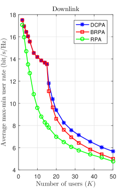
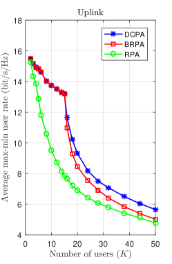
Figure 2: Average max-min rate per user versus the number of active MSs for different pilot allocation strategies ($N=64$ antennas, $L=8$ RF chains, ${C_{F}}_{d}={C_{F}}_{u}=64$ bit/s/Hz).

VII-A Impact of the pilot allocation process

Our aim in this subsection is to benchmark the performance of the proposed large-scale CSI-aware DCPA strategy against both the pure RPA and the BRPA schemes. Accordingly, the average max-min rate per user versus the number of active MSs is presented in Fig. 2 for each of these pilot allocation strategies and for both the DL and the UL. All results have been obtained assuming the default system parameters described in Table I, the use of $L=8$ RF chains fully connected to uniform linear antenna arrays with $N=64$ antenna elements, and fronthaul links with a capacity of ${C_{F}}_{d}={C_{F}}_{u}=64$ bit/s/Hz. The first important result to note from Fig. 2 is that the pure RPA scheme is clearly outperformed by both the BRPA and the DCPA strategies irrespective of the of active MSs in the network. In fact, the RPA scheme cannot guarantee neither the absence of pilot reuse, even for those cases in which $K\leq\tau_{p}$ (in this setup, $\tau_{p}=15$ time/frequency samples), nor the possibility of having pilots that are allocated to a high number of MSs and/or to MSs exhibiting very similar large-scale propagation patterns to the APs. Therefore, the higher the number of active MSs, the higher the probability of having one or more users suffering from high levels of pilot contamination, with the consequent reduction of the achievable max-min user rate. If we turn our attention to results provided by the BRPA and DCPA strategies, two disjoint operation regions can be distinguished. In the first one, comprising the scenarios in which $K\leq\tau_{p}$, both approaches allocate orthogonal pilots to the users (absence of pilot contamination) and thus naturally provide the same performance. In the second one, however, comprising the scenarios in which $K>\tau_{p}$, pilots have to be reused and, as a consequence, pilot contamination appears (note the rather abrupt performance drop when going from $K\leq\tau_{p}$ to $K>\tau_{p}$). In these scenarios, based on a smart exploitation of the available large-scale CSI, the proposed DCPA approach reduces the amount of pilot contamination experienced by the worst users in the network and it clearly improves the achievable max-min user rates provided by the channel-unaware BRPA scheme.

Another result that is worth emphasizing, since it will repeatedly appear in the following subsections, is that, although in scenarios with high-capacity fronthaul links the achievable max-min DL user rate is higher than that provided in the UL, as the number of active users in the network increases, the performance obtained in both the DL and the UL tend to become increasingly similar. This behavior can be easily deduced from the analysis of the SINR expressions in (36) and (39). As the number of active MSs in the cell-free network increases, provided that it is greater than $\tau_{p}$, the term in the denominator corresponding to the residual interuser interference due to pilot contamination becomes increasingly dominant in comparison to the quantification and thermal noise terms, eventually reaching the point where they can be considered virtually negligible. Under these conditions, and since the pre-coding filters used on both links are identical, the DL and the UL experience similar SINR values and, therefore, tend to provide the same achievable max-min rate per user, except for small differences that can be attributed to, on the one and, the dissimilar amount of quantified information that has to be conveyed through the corresponding fronthaul links and, on the other hand, disparities among the thermal noise powers experienced at both the APs and the MSs.

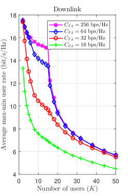
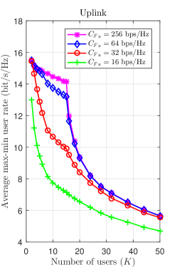
Figure 3: Average max-min rate per user versus the number of active MSs for different values of the fronthaul capacities ($N=64$ antennas, $L=8$ RF chains, DCPA).

VII-B Modifying the capacity of the fronthaul links and the RF infrastructure at the APs

The max-min achievable rate per user is plotted in Fig. 3 against the number of active MSs in the network, assuming the use of fronthaul links with different constraining capacities equal to 16, 32, 64 and 256 bit/s/Hz (for the network setups under consideration, using fronthaul links with a capacity of 256 bit/s/Hz is virtually equivalent to using infinite-capacity fronthauls). As expected, results show that increasing the fronthaul capacity is always beneficial if the main aim is to increase the achievable max-min user rate. Nevertheless, it is worth stressing that, keeping all the other parameters constant, the marginal increment of performance produced by each new increment of the fronthaul capacity suffers from the law of diminishing returns, especially for network setups with a high number of active MSs. That is, although the performance increase produced by doubling the fronthaul capacity from 16 bit/s/Hz to 32 bit/s/Hz, or even from 32 bit/s/Hz to 64 bit/s/Hz, can be justifiable, increasing the fronthaul capacity beyond 64 bit/s/Hz does not seem to be reasonable from the point of view of increasing the achievable performance of the system under the considered network setups. As observed in the previous subsection, in cell-free mmWave massive MIMO networks using high-capacity fronthaul links, the achievable max-min DL user rate is always slightly higher than that achieved in the UL irrespective of the number of active MSs. In scenarios with low-capacity fronthaul links and a large number of active MSs, however, the quantization noise experienced in the DL is higher than its UL counterpart and thus, the achievable per-user rate in the UL is slightly higher that than supplied in the DL.

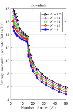
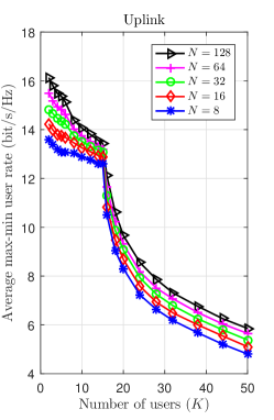
Figure 4: Average max-min rate per user versus the number of active MSs for different values of the number of antennas at the APs ($L=8$ RF chains, ${C_{F}}_{d}={C_{F}}_{u}=64$ bit/s/Hz, DCPA).

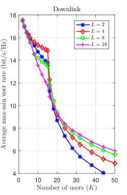
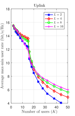
Figure 5: Average max-min rate per user versus the number of active MSs for different values of the number of RF chains at the APs ($N=64$ antennas, ${C_{F}}_{d}={C_{F}}_{u}=64$ bit/s/Hz, DCPA).

To understand how the RF infrastructure used at the APs influences the performance of the proposed cell-free mmWave massive MIMO system under constrained-capacity fronthaul links, Figs. 4 and 5 show the achievable max-min user rate against the number of active MSs assuming the use of uniform linear antenna arrays with different number of elements and fully-connected analog RF precoders with different number of RF chains, respectively. In particular, results presented in Fig. 4 have been obtained assuming the use of an analog precoder with $L=8$ RF chains fully-connected to a linear uniform antenna array with $N=8$, 16, 32, 64 or 128 antenna elements, whereas results presented in Fig. 5 have been obtained assuming the use of $L=2$, 4, 8 or 16 RF chains fully-connected to a linear uniform antenna array with $N=64$ antenna elements. The first conclusion we may draw when looking at the results presented in Fig. 4 is that, irrespective of the number of active MSs in the cell-free network, increasing the number of antenna elements at the APs in scenarios with high capacity fronthaul links (${C_{F}}_{d}={C_{F}}_{u}=64$ bit/s/Hz), although moderate and subject to the law of diminishing returns, always produces an increase in the achievable max-min user rate. As shown in Fig. 5, in contrast, the impact produced by an increase in the number of RF chains at the APs depends on the number of active MSs in the network. In particular, when the number of active users is high, the interuser interference term due to pilot contamination (imperfect CSI) dominates the factors in the denominator of the SINR (i.e., makes the quantization and thermal noises negligible) and thus, increasing the number of RF chains is always beneficial when trying to increase the achievable max-min user rate. When the number of active users in the network is low, however, the quantization noise, which is an increasing function of $L$, is not negligible anymore when compared to the interuser interference term (recall that this term is null when the number of active MSs is less than or equal to $\tau_{p}$) and thus, increasing the number of RF chains at the APs can be clearly disadvantageous.

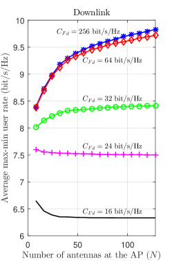
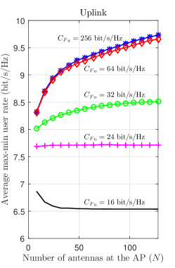
Figure 6: Average max-min rate per user versus the number of antennas at the APs for different values of the fronthaul capacities ($K=20$ users, $L=8$ RF chains, DCPA).

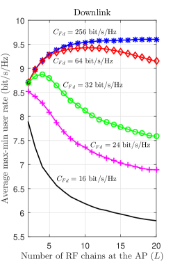
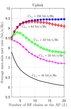
Figure 7: Average max-min rate per user versus the number of RF chains at the APs for different values of the fronthaul capacities ($K=20$ users, $N=64$ antennas, DCPA).

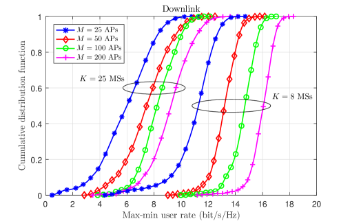
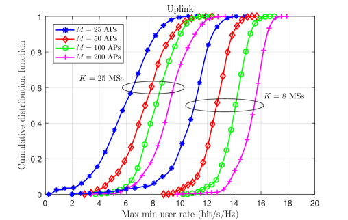
Figure 8: CDF of the DL and UL achievable max-min rate per user for different values of the number of APs and active MSs in the cell-free network ($N=64$ antennas, $L=8$ RF chains, ${C_{F}}_{d}={C_{F}}_{u}=64$ bit/s/Hz, DCPA).

Results presented in Figs. 3, 4 and 5 were obtained assuming high-capacity fronthaul links with ${C_{F}}_{d}={C_{F}}_{u}=64$ bit/s/Hz. However, the amount of quantized data that has to be conveyed from (to) the CPU to (from) the APs in the DL (UL) depends on the number of antennas and RF chains at the APs (see Section IV). Thus, in order to deepen in the study of the impact the RF infrastructure may have on the achievable performance of the proposed cell-free mmWave massive MIMO system under constrained-capacity fronthaul links, the average max-min user rate is plotted in Figs. 6 and 7 against the number of antenna elements and RF chains, respectively, for different values of the fronthaul capacities and assuming a fixed number of $K=20$ active MSs in the network. In network setups using very high capacity fronthaul links (i.e., ${C_{F}}_{d}={C_{F}}_{u}=256$ bit/s/Hz), increasing the number of antenna elements $N$ and/or the number of RF chains $L$ (up to $L=K$) is always beneficial as, in this case, the noise introduced by the quantization process is negligible and the system can take full advantage of the increased RF resources. As the capacity of the fronthaul links decreases, however, the amount of noise introduced by the quantization process increases with both $N$ and $L$ and, therefore, a situation arises where the potential performance improvement provided by the increase of $N$ and/or $L$ is compromised by the performance reduction due to fronthaul capacity constraints. On the one hand, it can be observed in Fig. 6 that, for fixed numbers of users and RF chains, there is a certain fronthaul capacity constraint value (near 24 bit/s/Hz in the setup used in this experiment) under which increasing the number of antenna elements at the array is counterproductive. On the other hand, results presented in Fig. 7 show that, for fixed numbers of users and antenna elements at the arrays, there is always an optimal number of RF chains to be deployed (or activated) at the APs that is dependent on the capacity of the fronthaul links. In particular, for the network setups under consideration, the optimal number of RF chains is equal to $L=10$, 4, and 1 when using fronthaul links with a capacity of 64 bit/s/Hz, 32 bit/s/Hz and less than 24 bit/s/Hz, respectively.

VII-C Impact of the density of APs

With the aim of evaluating the impact the density of APs per area unit may have on the performance of the proposed cell-free mmWave massive MIMO system, Fig. 8 represents the cumulative distribution function (CDF) of the DL and UL achievable max-min user rate for different values of the number of APs in the network. It has been assumed in these experiments a fixed number of active MSs equal to either $K=25$ or $K=8$ MSs, the use of $L=8$ RF chains fully-connected to a linear uniform antenna array with $N=64$ antenna elements, and the use of DL and UL fronthaul links with a capacity ${C_{F}}_{d}={C_{F}}_{u}=64$ bit/s/Hz. As expected, cell-free massive MIMO scenarios with a high density of APs per area unit significantly outperform those with a low density of APs per area unit in both median and 95%-likely achievable per-user rate performance. However, the achievable max-min user rate increase due to increasing the number of APs in the network is, again, subject to the law of diminishing returns. For instance, in scenarios with $K=25$ MSs, the 95%-likely achievable user rate is equal to 2.55, 4.33, 6.11 and 6.50 bit/s/Hz for cell-frre massive MIMO networks with $M=25$, 50, 100 and 200 APs, respectively. That is, doubling the number of APs per area unit does not result in doubling the 95%-likely achievable user rate. Similar conclusions can be drawn when looking at either the median or the average achievable user rates.

As was observed in results presented in previous subsections for high-capacity fronthaul setups, when the number of active users in the system is low, the achievable max-min rate values in the DL are slightly higher than those achievable in the UL. Instead, when the number of active users increases, the achievable max-min user rates are virtually identical in both the DL and the UL. Also, note that the dispersion of the achievable max-min user rates around the median tends to diminish as the density of APs increases. That is, cell-free massive MIMO networks with a high density of APs per area unit tend to offer max-min achievable rates that suffer little variations irrespective of the location of the APs (i.e, irrespective of the scenario under evaluation).

VIII Conclusion

A novel analytical framework for the performance analysis of cell-free mmWave massive MIMO networks has been introduced in this paper. The proposed framework considers the use of low-complexity hybrid precoders/decoders where the RF high-dimensionality phase shifter-based precoding/decoding stage is based on large-scale second-order channel statistics, while the low-dimensionality baseband multiuser MIMO precoding/decoding stage can be easily implemented by standard ZF signal processing schemes using small-scale estimated CSI. Furthermore, it also takes into account the impact of using capacity-constrained fronthaul links that assume the use of large-block lattice quantization codes able to approximate a Gaussian quantization noise distribution, which constitutes an upper bound to the performance attained under any practical quantization scheme. Max-min power allocation and fronthaul quantization optimization problems have been posed thanks to the development of mathematically tractable expressions for both the per-user achievable rates and the fronthaul capacity consumption. These optimization problems have been solved by combining the use of block coordinate descent methods with sequential linear optimization programs. Results have shown that the proposed DCPA suboptimal pilot allocation strategy, which is based on the idea of clustering by dissimilarity, overcomes the computational burden of the optimal small-scale CSI-based pilot allocation scheme while clearly outperforming the pure random and balanced random schemes. It has also been shown that, although increasing the fronthaul capacity and/or the density of APs per area unit is always beneficial from the point of view of the achievable max-min user rate, the marginal increment of performance produced by each new increment of these parameters suffers from the law of diminishing returns, especially for network setups with a high number of active MSs. Moreover, simulation results indicate that, as the capacity of the fronthaul links decreases, the potential performance improvement provided by the increase of the number of antenna elements $N$ and/or the number of RF chains $L$ is compromised by the performance reduction due to the corresponding increase of the fronthaul quantization noise. In particular, for fixed numbers of users and RF chains, there is a certain fronthaul capacity constraint value (near 24 bit/s/Hz in the setups under consideration) under which increasing the number of antenna elements at the array is counterproductive. Similarly, for fixed numbers of users and antenna elements at the arrays, there is always an optimal number of RF chains to be deployed (or activated) at the APs that is dependent on the capacity of the fronthaul links. For future work, it would be interesting to develop low-complexity pilot- and power-allocation techniques specifically designed to maximize the energy efficiency of cell-free mmWave massive MIMO networks considering both the fronthaul capacity constraints and the fronthaul power consumption. It would also be interesting to explore the use of partially-connected RF precoding/decoding architectures and the implementation of baseband MU-MIMO precoding/decoding other than the ZF scheme.

Appendix A Proof of Theorem 38

Following an approach similar to that proposed by Nayebi et al. in [17], the signal received by the $k$th MS in (29) can be rewritten as ${y_{d}}_{k}={y_{d}}_{k\,0}+{y_{d}}_{k\,1}+{y_{d}}_{k\,2}+{n_{d}}_{k}$, where the useful, interuser interference, and quantization noise terms can be expressed as ${y_{d}}_{k\,0}=\sqrt{\upsilon_{k}}{s_{d}}_{k}$, ${y_{d}}_{k\,1}=\tilde{\boldsymbol{g}}_{k}^{T}\boldsymbol{W}_{d}^{BB}\boldsymbol{\Upsilon}^{1/2}\boldsymbol{s}_{d}$, and ${y_{d}}_{k\,2}=\boldsymbol{g}_{k}^{T}\boldsymbol{q}_{d}=\sum_{m=1}^{M}\boldsymbol{g}_{km}^{T}{\boldsymbol{q}_{d}}_{m}$, respectively. Now, considering that data symbols, quantization noise, thermal noise, and channel-related coefficients are mutually independent, the terms ${y_{d}}_{k\,0}$, ${y_{d}}_{k\,1}$, ${y_{d}}_{k\,2}$ and ${n_{d}}_{k}$ are mutually uncorrelated and thus, based on the worst-case uncorrelated additive noise [40], the achievable DL rate for user $k$ is lower bounded by ${R_{d}}_{k}=\log_{2}\left(1+{\operatorname{SINR}_{d}}_{k}\right)$, with

$${\operatorname{SINR}_{d}}_{k}=\frac{\mathbb{E}\left\{\left|{y_{d}}_{k\,0}\right|^{2}\right\}}{\mathbb{E}\left\{\left|{y_{d}}_{k\,1}\right|^{2}\right\}+\mathbb{E}\left\{\left|{y_{d}}_{k\,2}\right|^{2}\right\}+\sigma_{d}^{2}},$$

where $\mathbb{E}\left\{\left|{y_{d}}_{k\,0}\right|^{2}\right\}=\upsilon_{k}$,

$$\begin{split}&\mathbb{E}\left\{\left|{y_{d}}_{k\,1}\right|^{2}\right\}=\mathbb{E}\left\{\boldsymbol{s}_{d}^{H}\boldsymbol{\Upsilon}^{1/2}{\boldsymbol{W}_{d}^{BB}}^{H}\tilde{\boldsymbol{g}}_{k}^{*}\tilde{\boldsymbol{g}}_{k}^{T}\boldsymbol{W}_{d}^{BB}\boldsymbol{\Upsilon}^{1/2}\boldsymbol{s}_{d}\right\}\\ &\qquad=\operatorname{tr}\left(\boldsymbol{\Upsilon}\mathbb{E}\left\{{\boldsymbol{W}_{d}^{BB}}^{H}\tilde{\boldsymbol{g}}_{k}^{*}\tilde{\boldsymbol{g}}_{k}^{T}\boldsymbol{W}_{d}^{BB}\right\}\right)\\ &\qquad=\sum_{k^{\prime}=1}^{K}\upsilon_{k^{\prime}}\left[\operatorname{diag}\left(\mathbb{E}\left\{{\boldsymbol{W}_{d}^{BB}}^{H}\tilde{\boldsymbol{g}}_{k}^{*}\tilde{\boldsymbol{g}}_{k}^{T}\boldsymbol{W}_{d}^{BB}\right\}\right)\right]_{k^{\prime}},\end{split}$$

and

$$\begin{split}\mathbb{E}\left\{\left|{y_{d}}_{k\,2}\right|^{2}\right\}&=\sum_{m=1}^{M}\mathbb{E}\left\{{\boldsymbol{q}_{d}}_{m}^{H}\boldsymbol{g}_{km}^{*}\boldsymbol{g}_{km}^{T}{\boldsymbol{q}_{d}}_{m}\right\}\\ &=\sum_{m=1}^{M}{\sigma_{q}^{2}}_{dm}\operatorname{tr}\left(\boldsymbol{R}_{mk}^{RF}\right).\end{split}$$

Appendix B Proof of Theorem 43

The detected signal at the CPU corresponding to the symbol transmitted by the $k$th MS in (35) can be rewritten as ${y_{u}}_{k}={y_{u}}_{k\,0}+{y_{u}}_{k\,1}+{y_{u}}_{k\,2}+{y_{u}}_{k\,3}$, where the useful, interuser interference, quantization noise and thermal noise terms can be expressed as ${y_{u}}_{k\,0}=\sqrt{P_{u}}\sqrt{\omega_{k}}{s_{u}}_{k}$, ${y_{u}}_{k\,1}=\sqrt{P_{u}}\left[\boldsymbol{W}_{u}^{BB}\tilde{\boldsymbol{G}}\boldsymbol{\Omega}^{1/2}\boldsymbol{s}_{u}\right]_{k}$, ${y_{u}}_{k\,2}=\left[\boldsymbol{W}_{u}^{BB}\boldsymbol{q}_{u}\right]_{k}$, and ${y_{u}}_{k\,3}=\left[\boldsymbol{W}_{u}^{BB}\boldsymbol{n}_{u}\right]_{k}$, respectively. As in the DL, since data symbols, quantization noise, thermal noise, and channel-related coefficients are mutually independent, the terms ${y_{u}}_{k\,0}$, ${y_{u}}_{k\,1}$, ${y_{d}}_{k\,2}$ and ${y_{d}}_{k\,3}$ are mutually uncorrelated and thus, based on the worst-case uncorrelated additive noise [40], the achievable UL rate for user $k$ is lower bounded by ${R_{u}}_{k}=\log_{2}\left(1+{\operatorname{SINR}_{u}}_{k}\right)$, with

$${\operatorname{SINR}_{u}}_{k}=\frac{\mathbb{E}\left\{\left|{y_{d}}_{k\,0}\right|^{2}\right\}}{\mathbb{E}\left\{\left|{y_{d}}_{k\,1}\right|^{2}\right\}+\mathbb{E}\left\{\left|{y_{d}}_{k\,2}\right|^{2}\right\}+\mathbb{E}\left\{\left|{y_{d}}_{k\,3}\right|^{2}\right\}},$$

where $\mathbb{E}\left\{\left|{y_{u}}_{k\,0}\right|^{2}\right\}=P_{u}\omega_{k}$,

$$\begin{split}&\mathbb{E}\left\{\left|{y_{u}}_{k\,1}\right|^{2}\right\}=P_{u}\mathbb{E}\left\{\boldsymbol{s}_{u}^{H}\boldsymbol{\Omega}^{1/2}\tilde{\boldsymbol{G}}^{H}{\boldsymbol{w}_{uk}^{BB}}^{H}\boldsymbol{w}_{uk}^{BB}\tilde{\boldsymbol{G}}\boldsymbol{\Omega}^{1/2}\boldsymbol{s}_{u}\right\}\\ &\qquad=P_{u}\operatorname{tr}\left(\boldsymbol{\Omega}\mathbb{E}\left\{\tilde{\boldsymbol{G}}^{H}{\boldsymbol{w}_{uk}^{BB}}^{H}\boldsymbol{w}_{uk}^{BB}\tilde{\boldsymbol{G}}\right\}\right)\\ &\qquad=P_{u}\sum_{k^{\prime}=1}^{K}\omega_{k^{\prime}}\left[\operatorname{diag}\left(\mathbb{E}\left\{\tilde{\boldsymbol{G}}^{H}{\boldsymbol{w}_{uk}^{BB}}^{H}\boldsymbol{w}_{uk}^{BB}\tilde{\boldsymbol{G}}\right\}\right)\right]_{k^{\prime}},\end{split}$$

with $\boldsymbol{w}_{uk}^{BB}$ denoting the $k$th row of $\boldsymbol{W}_{u}^{BB}$, or, equivalently,

$$\begin{split}&\mathbb{E}\left\{\left|{y_{u}}_{k\,1}\right|^{2}\right\}=P_{u}\left[\operatorname{diag}\left(\mathbb{E}\left\{\boldsymbol{W}_{u}^{BB}\tilde{\boldsymbol{G}}\boldsymbol{\Omega}\tilde{\boldsymbol{G}}^{H}{\boldsymbol{W}_{u}^{BB}}^{H}\right\}\right)\right]_{k}\\ &\qquad=P_{u}\sum_{k^{\prime}=1}^{K}\omega_{k^{\prime}}\left[\operatorname{diag}\left(\mathbb{E}\left\{\boldsymbol{W}_{u}^{BB}\tilde{\boldsymbol{g}}_{k^{\prime}}\tilde{\boldsymbol{g}}_{k^{\prime}}^{H}{\boldsymbol{W}_{u}^{BB}}^{H}\right\}\right)\right]_{k},\end{split}$$

and, finally,

$$\begin{split}&\mathbb{E}\left\{\left|{y_{u}}_{k\,2}\right|^{2}\right\}=\left[\operatorname{diag}\left(\mathbb{E}\left\{\boldsymbol{W}_{u}^{BB}\boldsymbol{q}_{u}\boldsymbol{q}_{u}^{H}{\boldsymbol{W}_{u}^{BB}}^{H}\right\}\right)\right]_{k}\\ &\qquad=\sum_{m=1}^{M}\left[\operatorname{diag}\left(\mathbb{E}\left\{\boldsymbol{W}_{u}^{BB}\boldsymbol{q}_{um}\boldsymbol{q}_{um}^{H}{\boldsymbol{W}_{u}^{BB}}^{H}\right\}\right)\right]_{k}\\ &\qquad=\sum_{m=1}^{M}{\sigma_{q}^{2}}_{um}\left[\operatorname{diag}\left(\mathbb{E}\left\{\boldsymbol{W}_{u\,m}^{BB}{\boldsymbol{W}_{u\,m}^{BB}}^{H}\right\}\right)\right]_{k},\end{split}$$

and, analogously,

$$\begin{split}\mathbb{E}\left\{\left|{y_{d}}_{k\,3}\right|^{2}\right\}=\sigma_{u}^{2}(N)\sum_{m=1}^{M}\left[\operatorname{diag}\left(\mathbb{E}\left\{\boldsymbol{W}_{u\,m}^{BB}{\boldsymbol{W}_{u\,m}^{BB}}^{H}\right\}\right)\right]_{k}.\end{split}$$

References

- [1] M. Shafi, A. F. Molisch, P. J. Smith, T. Haustein, P. Zhu, P. D. Silva, F. Tufvesson, A. Benjebbour, and G. Wunder, “5G: A tutorial overview of standards, trials, challenges, deployment, and practice,” IEEE Journal on Selected Areas in Communications, vol. 35, no. 6, pp. 1201–1221, June 2017.
- [2] K. David and H. Berndt, “6G vision and requirements: Is there any need for beyond 5G?” IEEE Vehicular Technology Magazine, vol. 13, no. 3, pp. 72–80, Sept 2018.
- [3] T. L. Marzetta, E. G. Larsson, H. Yang, and H. Q. Ngo, Fundamentals of massive MIMO. Cambridge University Press, 2016.
- [4] T. L. Marzetta, “Noncooperative cellular wireless with unlimited numbers of base station antennas,” IEEE Transactions on Wireless Communications, vol. 9, no. 11, pp. 3590–3600, November 2010.
- [5] M. K. Karakayali, G. J. Foschini, and R. A. Valenzuela, “Network coordination for spectrally efficient communications in cellular systems,” IEEE Wireless Communications, vol. 13, no. 4, pp. 56–61, Aug 2006.
- [6] D. Gesbert, S. Hanly, H. Huang, S. S. Shitz, O. Simeone, and W. Yu, “Multi-cell MIMO cooperative networks: A new look at interference,” IEEE Journal on Selected Areas in Communications, vol. 28, no. 9, pp. 1380–1408, December 2010.
- [7] R. Irmer, H. Droste, P. Marsch, M. Grieger, G. Fettweis, S. Brueck, H. Mayer, L. Thiele, and V. Jungnickel, “Coordinated multipoint: Concepts, performance, and field trial results,” IEEE Communications Magazine, vol. 49, no. 2, pp. 102–111, February 2011.
- [8] A. Checko, H. L. Christiansen, Y. Yan, L. Scolari, G. Kardaras, M. S. Berger, and L. Dittmann, “Cloud RAN for mobile networks - A technology overview,” IEEE Communications Surveys Tutorials, vol. 17, no. 1, pp. 405–426, Firstquarter 2015.
- [9] H. Q. Ngo, A. Ashikhmin, H. Yang, E. G. Larsson, and T. L. Marzetta, “Cell-free massive MIMO: Uniformly great service for everyone,” in IEEE SPAWC 2015.
- [10] ——, “Cell-free massive MIMO versus small cells,” IEEE Transactions on Wireless Communications, vol. 16, no. 3, pp. 1834–1850, 2017.
- [11] T. S. Rappaport, S. Sun, R. Mayzus, H. Zhao, Y. Azar, K. Wang, G. N. Wong, J. K. Schulz, M. Samimi, and F. Gutierrez, “Millimeter wave mobile communications for 5G cellular: It will work!” IEEE Access, vol. 1, pp. 335–349, May 2013.
- [12] F. Boccardi, R. W. Heath, A. Lozano, T. L. Marzetta, and P. Popovski, “Five disruptive technology directions for 5G,” IEEE Communications Magazine, vol. 52, no. 2, pp. 74–80, February 2014.
- [13] M. R. Akdeniz, Y. Liu, M. K. Samimi, S. Sun, S. Rangan, T. S. Rappaport, and E. Erkip, “Millimeter wave channel modeling and cellular capacity evaluation,” IEEE Journal on Selected Areas in Communications, vol. 32, no. 6, pp. 1164–1179, 2014.
- [14] T. S. Rappaport, Y. Xing, G. R. MacCartney, A. F. Molisch, E. Mellios, and J. Zhang, “Overview of millimeter wave communications for fifth-generation (5G) wireless networks - with a focus on propagation models,” IEEE Transactions on Antennas and Propagation, vol. 65, no. 12, pp. 6213–6230, Dec 2017.
- [15] X. Gao, L. Dai, and A. M. Sayeed, “Low RF-complexity technologies to enable millimeter-wave MIMO with large antenna array for 5G wireless communications,” IEEE Communications Magazine, vol. 56, no. 4, pp. 211–217, April 2018.
- [16] S. A. Busari, K. M. S. Huq, S. Mumtaz, L. Dai, and J. Rodriguez, “Millimeter-wave massive MIMO communication for future wireless systems: A survey,” IEEE Communications Surveys Tutorials, vol. 20, no. 2, pp. 836–869, Second quarter 2018.
- [17] E. Nayebi, A. Ashikhmin, T. L. Marzetta, H. Yang, and B. D. Rao, “Precoding and power optimization in cell-free massive MIMO systems,” IEEE Transactions on Wireless Communications, vol. 16, no. 7, pp. 4445–4459, July 2017.
- [18] L. D. Nguyen, T. Q. Duong, H. Q. Ngo, and K. Tourki, “Energy efficiency in cell-free massive MIMO with zero-forcing precoding design,” IEEE Communications Letters, vol. 21, no. 8, pp. 1871–1874, Aug 2017.
- [19] H. Q. Ngo, L. Tran, T. Q. Duong, M. Matthaiou, and E. G. Larsson, “On the total energy efficiency of cell-free massive MIMO,” IEEE Transactions on Green Communications and Networking, vol. 2, no. 1, pp. 25–39, March 2018.
- [20] M. Bashar, K. Cumanan, A. G. Burr, H. Q. Ngo, and M. Debbah, “Cell-free massive MIMO with limited backhaul,” arXiv preprint arXiv:1801.10190, 2018.
- [21] M. N. Boroujerdi, A. Abbasfar, and M. Ghanbari, “Cell free massive MIMO with limited capacity fronthaul,” Wireless Personal Communications, October 2018.
- [22] O. E. Ayach, S. Rajagopal, S. Abu-Surra, Z. Pi, and R. W. Heath, “Spatially sparse precoding in millimeter wave MIMO systems,” IEEE Transactions on Wireless Communications, vol. 13, no. 3, pp. 1499–1513, March 2014.
- [23] X. Gao, L. Dai, S. Han, C. I, and R. W. Heath, “Energy-efficient hybrid analog and digital precoding for mmWave MIMO systems with large antenna arrays,” IEEE Journal on Selected Areas in Communications, vol. 34, no. 4, pp. 998–1009, April 2016.
- [24] A. F. Molisch, V. V. Ratnam, S. Han, Z. Li, S. L. H. Nguyen, L. Li, and K. Haneda, “Hybrid beamforming for massive MIMO: A survey,” IEEE Communications Magazine, vol. 55, no. 9, pp. 134–141, Sept 2017.
- [25] S. Park, A. Alkhateeb, and R. W. Heath, “Dynamic subarrays for hybrid precoding in wideband mmWave MIMO systems,” IEEE Transactions on Wireless Communications, vol. 16, no. 5, pp. 2907–2920, May 2017.
- [26] M. Alonzo and S. Buzzi, “Cell-free and user-centric massive MIMO at millimeter wave frequencies,” in IEEE International Symposium on Personal, Indoor, and Mobile Radio Communications (PIMRC), Oct 2017, pp. 1–5.
- [27] M. Alonzo, S. Buzzi, and A. Zappone, “Energy-efficient downlink power control in mmwave cell-free and user-centric massive MIMO,” CoRR, vol. abs/1805.05177, 2018. [Online]. Available: http://arxiv.org/abs/1805.05177
- [28] M. K. Samimi and T. S. Rappaport, “Ultra-wideband statistical channel model for non line of sight millimeter-wave urban channels,” in 2014 IEEE Global Communications Conference, Dec 2014, pp. 3483–3489.
- [29] A. Adhikary, E. A. Safadi, M. K. Samimi, R. Wang, G. Caire, T. S. Rappaport, and A. F. Molisch, “Joint spatial division and multiplexing for mm-Wave channels,” IEEE Journal on Selected Areas in Communications, vol. 32, no. 6, pp. 1239–1255, June 2014.
- [30] R. Méndez-Rial, N. González-Prelcic, and R. W. Heath, “Adaptive hybrid precoding and combining in MmWave multiuser MIMO systems based on compressed covariance estimation,” in IEEE 6th International Workshop on Computational Advances in Multi-Sensor Adaptive Processing (CAMSAP), Dec 2015, pp. 213–216.
- [31] S. Park and R. W. Heath, “Spatial channel covariance estimation for mmWave hybrid MIMO architecture,” in Asilomar Conference on Signals, Systems and Computers, Nov 2016, pp. 1424–1428.
- [32] S. Park and R. W. Heath Jr, “Spatial channel covariance estimation for the hybrid MIMO architecture: A compressive sensing based approach,” arXiv preprint arXiv:1711.04207, 2017.
- [33] S. Park, J. Park, A. Yazdan, and R. W. Heath, “Exploiting spatial channel covariance for hybrid precoding in massive MIMO systems,” IEEE Transactions on Signal Processing, vol. 65, no. 14, pp. 3818–3832, July 2017.
- [34] R. Mai, T. Le-Ngoc, and D. H. N. Nguyen, “Two-timescale hybrid RF-baseband precoding with MMSE-VP for multi-user massive MIMO broadcast channels,” IEEE Transactions on Wireless Communications, vol. 17, no. 7, pp. 4462–4476, July 2018.
- [35] Z. Shen, R. Chen, J. G. Andrews, R. W. Heath, and B. L. Evans, “Low complexity user selection algorithms for multiuser MIMO systems with block diagonalization,” IEEE Transactions on Signal Processing, vol. 54, no. 9, pp. 3658–3663, 2006.
- [36] O. Elijah, C. Y. Leow, T. A. Rahman, S. Nunoo, and S. Z. Iliya, “A comprehensive survey of pilot contamination in massive MIMO-5G system,” IEEE Comm. Surv. & Tutor., vol. 18, no. 2, pp. 905–923, 2016.
- [37] L. Lu, G. Y. Li, A. L. Swindlehurst, A. Ashikhmin, and R. Zhang, “An overview of massive MIMO: Benefits and challenges,” IEEE Journal of Selected Topics in Signal Processing, vol. 8, no. 5, pp. 742–758, 2014.
- [38] R. Zamir and M. Feder, “On lattice quantization noise,” IEEE Transactions on Information Theory, vol. 42, no. 4, pp. 1152–1159, Jul 1996.
- [39] G. Femenias and F. Riera-Palou, “Multi-layer downlink precoding for cloud-RAN systems using full-dimensional massive MIMO,” IEEE Access, vol. 6, pp. 61 583–61 599, 2018.
- [40] B. Hassibi and B. M. Hochwald, “How much training is needed in multiple-antenna wireless links?” IEEE Transactions on Information Theory, vol. 49, no. 4, pp. 951–963, April 2003.
- [41] H. Yang and T. L. Marzetta, “Capacity performance of multicell large-scale antenna systems,” in 51st Annual Allerton Conference on Communication, Control, and Computing (Allerton), Oct 2013, pp. 668–675.
- [42] G. Interdonato, H. Q. Ngo, E. G. Larsson, and P. Frenger, “On the performance of cell-free massive MIMO with short-term power constraints,” in IEEE 21st International Workshop on Computer Aided Modelling and Design of Communication Links and Networks (CAMAD), Oct 2016, pp. 225–230.
- [43] T. M. Cover and J. A. Thomas, Elements of Information Theory (Wiley Series in Telecommunications and Signal Processing), 2nd ed. Wiley-Interscience, 2006.
- [44] H. Ahmadi, A. Farhang, N. Marchetti, and A. MacKenzie, “A game theoretic approach for pilot contamination avoidance in massive MIMO,” IEEE Wireless Communications Letters, vol. 5, no. 1, pp. 12–15, 2016.
- [45] P. Tseng, “Convergence of a block coordinate descent method for nondifferentiable minimization,” Journal of Optimization Theory and Applications, vol. 109, no. 3, pp. 475–494, June 2001.
- [46] A. Beck and L. Tetruashvili, “On the convergence of block coordinate descent type methods,” SIAM Journal on Optimization, vol. 23, no. 4, pp. 2037–2060, 2013.