FFT-based homogenisation accelerated by low-rank tensor approximations

Abstract

Fast Fourier transform (FFT) based methods have turned out to be an effective computational approach for numerical homogenisation. In particular, Fourier-Galerkin methods are computational methods for partial differential equations that are discretised with trigonometric polynomials. Their computational effectiveness benefits from efficient FFT based algorithms as well as a favourable condition number. Here these kind of methods are accelerated by low-rank tensor approximation techniques for a solution field using canonical polyadic, Tucker, and tensor train formats. This reduced order model also allows to efficiently compute suboptimal global basis functions without solving the full problem. It significantly reduces computational and memory requirements for problems with a material coefficient field that admits a moderate rank approximation. The advantages of this approach against those using full material tensors are demonstrated using numerical examples for the model homogenisation problem that consists of a scalar linear elliptic variational problem defined in two and three dimensional settings with continuous and discontinuous heterogeneous material coefficients. This approach opens up the potential of an efficient reduced order modelling of large scale engineering problems with heterogeneous material.

Keywords: Fourier-Galerkin method, fast Fourier transform, low-rank approximations, reduced order modelling, homogenisation

1 Introduction

FFT-based methods. A fast Fourier transform (FFT) based method has been introduced as an efficient algorithm for numerical homogenisation in 1994 by Moulinec and Suquet [1]. The method, that has application in multiscale problems, represents an alternative discretisation approach to the finite element method. The effectiveness of FFT-based homogenisation relies on the facts that the system matrix is never assembled, the matrix-vector product in linear iterative solvers is provided very efficiently by FFT, and the condition number is independent of discretisation parameters.

Since the seminal paper in 1994 the methodology has been significantly developed. Originally the approach has been based on Lippmann-Schwinger equation, which is a formulation incorporating Green’s function for an auxiliary homogeneous problem. Its connection to a standard variational formulation has been discovered in [2] by using the fact that Green’s function is a projection on compatible fields (i.e. gradient fields in scalar elliptic problems), see [3]. It has allowed to fully remove the reference conductivity tensor from the formulation, and interpreted the method from the perspective of finite elements also in nonlinear problems [4, 5]. Moreover, the standard primal-dual variational formulations allow to compute guaranteed bounds on effective material properties [6], which provides tighter bounds than the Hashin-Shtrikman functional.

Significant attention has been focused on developing discretisation approaches that justify the original FFT-based homogenisation algorithm. Many efforts have been made on discretisation with trigonometric polynomials, starting with [7] and followed by [6, 8, 4, 9]. Other discretisation approaches are based on pixel-wise constant basis functions [10, 11], linear hexahedral elements [12], or finite differences [13, 14]. The variational formulations also allowed to derive convergence of approximate solutions to the continuous one [2, 9, 10].

The various discretisation approaches have been studied along with linear and non-linear solvers [15, 16, 7, 17, 11, 18, 4, 5, 19]. Other research directions focus, for example, on multiscale methods [20, 21, 22], highly non-linear problems in solid mechanics [23, 24, 25, 26], and parameter estimation features FFT and model reduction [27].

Low-rank approximations. The general idea of low-rank approximations is to express or compress tensors with fewer parameters, which can lead to a huge reduction in requirements for computer memory and possible significant computational speed-up. For matrices as second order tensors, the optimal low-rank approximation in mean square sense is based on the truncated singular value decomposition (SVD). A computationally cheaper choice is Cross Approximation [28, 29] which has only linear complexity in matrix size $N$. Low-rank formats or tensors of order larger than two include the canonical polyadic (CP), Tucker, and hierarchical schemes such as the tensor train and the quantic tensor-train form of [30, 31]. Low-rank formats are not only needed to compress the data tensor as the final delivered result of high-dimensional numerical modellings, but are also preferred to approximate tensors in the numerical solution process. In [32] the proper generalised decomposition is adopted for the construction of low-rank tensors in CP and Tucker formats in a numerical homogenisation from high-resolution images. It is also possible to compute the tensors directly in low-rank formats, which can be provided by a suitable solver [33, 34, 35, 36, 37]. The rank one tensors in low-rank approximations can be seen as suboptimal global basis functions.

However, the need to compute with tensors in low-rank formats requires one to deal with operations such as addition, element-wise multiplication, or Fourier transformation. Since the low-rank tensors are described with fewer parameters, the computational complexities are typically reduced, which may lead to significant speed-up of computations. However, performing such operations with tensors in low-rank format, it typically happens that the representation rank of the tensors grows, which calls for their truncation, i.e. their approximation or reparametrisation with fewer parameters while keeping a reasonable accuracy [38, 39, 40]. This truncation of tensors may be viewed as a generalisation of the rounding of numbers, which occurs when working with floating point formats. In general, the applications of low-rank approximations are very broad, e.g. for stochastic problems with high number of random parameters [41, 37, 42, 43], acceleration of solutions to PDEs [44, 45], or model order reduction [46], but its application to FFT-based homogenisation is new. However, an alternative low-rank representation has been studied recently in [47].

Structure of the paper. In section 2, two state-of-the-art Fourier-Galerkin methods are described for a model homogenisation problem of a scalar elliptic equation. In particular, the two discretisation methods based on numerical and exact integration are described along with their corresponding linear systems. Then in section LABEL:sec:fft-based-methods-with-low-rank-approximations the low-rank approximation techniques are summarised and their application within a Fourier-Galerkin method is discussed. In section LABEL:sec:numerical-results, the effectiveness of low-rank approximations is demonstrated on several numerical examples.

Notation. We will denote vectors and matrices by boldface letters: $\boldsymbol{a}=\left(a_{i}\right)_{i=1,2,\ldots,d}\in\mathbb{R}^{d}$ or $\boldsymbol{A}=(A_{ij})_{i,j=1}^{d}\in\mathbb{R}^{d\times d}$. Matrix-matrix and matrix-vector multiplications are denoted as $\boldsymbol{C}=\boldsymbol{A}\boldsymbol{B}$ and $\boldsymbol{c}=\boldsymbol{A}\boldsymbol{b}$, which in Einstein summation notation reads $C_{ik}=A_{ij}B_{jk}$ and $b_{i}=A_{ij}b_{j}$ respectively. The Euclidean inner product will be referred to as $\boldsymbol{a}\cdot\boldsymbol{\bar{b}}=\sum_{i}a_{i}\overline{b}_{i}$, and the induced norm as $\|\boldsymbol{a}\|=\sqrt{\boldsymbol{a}\cdot\boldsymbol{\bar{a}}}$. Vectors, matrices, and tensors such as $\boldsymbol{\mathsfit{x}}$, $\boldsymbol{\mathsfit{b}}$, and $\boldsymbol{\mathsfit{A}}$ arising from discretisation will be denoted by the bold sans-serif font in order to highlight their special structure. For ${\boldsymbol{N}}=(N_{1},\dotsc,N_{d})\in\mathbb{N}^{d}$, the components of a tensor $\boldsymbol{\mathsfit{A}}\in\mathbb{R}^{{\boldsymbol{N}}}=\bigotimes_{\alpha=1}^{d}\mathbb{R}^{N_{\alpha}}$ of order $d$ will be denoted as $\mathsfit{A}[k_{1},...,k_{d}]$. The multiindex notation will be also incorporated to simplify the components of the tensors, e.g. $\mathsfit{A}[k_{1},...,k_{d}]=\mathsfit{A}[\boldsymbol{k}]$ for a multi-index $\boldsymbol{k}=[k_{1},\dotsc,k_{d}]$. The space $\mathbb{R}^{\boldsymbol{N}}$, composed of tensors of order $d$, can be considered as a vector space, which allows to talk about its dimension as the number of basis vectors, i.e. $\dim\mathbb{R}^{\boldsymbol{N}}=\prod_{\alpha=1}^{d}N_{\alpha}$.

The space of square integrable $\mathcal{Y}$-periodic functions defined on a periodic cell $\mathcal{Y}=(-\frac{1}{2},\frac{1}{2})^{d}$ is denoted as $L^{2}(\mathcal{Y})$. The analogous space $L^{2}(\mathcal{Y};\mathbb{R}^{d})$ collects $\mathbb{R}^{d}$-valued functions ${\boldsymbol{v}}:\mathcal{Y}\rightarrow\mathbb{R}^{d}$ with components $v_{i}$ from $L^{2}(\mathcal{Y})$. Finally, $H^{1}_{0}(\mathcal{Y})=\{v\in L^{2}(\mathcal{Y})\,|\,\nabla v\in L^{2}(\mathcal{Y};\mathbb{R}^{d}),\int_{\mathcal{Y}}v(\boldsymbol{x})\,{\mathrm{d}}\boldsymbol{x}=0\}$ denotes the Sobolev space of periodic functions with zero mean.

2 Homogenisation by Fourier-Galerkin methods

2.1 Model problem

A model problem in homogenisation [48] consists of a scalar linear elliptic variational problem defined on a unit domain $\mathcal{Y}=(-\frac{1}{2},\frac{1}{2})^{d}$ in a spatial dimension $d$ (we consider both $d=2$ and $d=3$) with material coefficients $\boldsymbol{A}:\mathcal{Y}\rightarrow\mathbb{R}^{d\times d}$, which are required to be essentially bounded, symmetric, and uniformly elliptic. This means that for almost all $\boldsymbol{x}\in\mathcal{Y}$, there are constants $0<c_{A}\leq C_{A}<+\infty$ such that

$$\boldsymbol{A}(\boldsymbol{x}) =\boldsymbol{A}^{T}(\boldsymbol{x}), c_{A}\lVert{\boldsymbol{v}}\rVert^{2} \leq\boldsymbol{A}(\boldsymbol{x}){\boldsymbol{v}}\cdot{\boldsymbol{v}}\leq C_{A}\lVert{\boldsymbol{v}}\rVert^{2}\quad\text{ for all }{\boldsymbol{v}}\in\mathbb{R}^{d}.$$ (1)

The homogenisation problem is focused on the computation of effective material properties $\boldsymbol{A}_{\mathrm{H}}\in\mathbb{R}^{d\times d}$. Its variational formulation is based on the minimisation of a microscopic energetic functional for constant vectors $\boldsymbol{E}\in\mathbb{R}^{d}$, which represents an average of the macroscopic gradient, as

$$\boldsymbol{A}_{\mathrm{H}}\boldsymbol{E}\cdot\boldsymbol{E}=\min_{v\in H^{1}_{0}(\mathcal{Y})}a\bigl{(}\boldsymbol{E}+\nabla v,\boldsymbol{E}+\nabla v\bigr{)},$$ (2)

where the bilinear form $a:L^{2}(\mathcal{Y};\mathbb{R}^{d})\times L^{2}(\mathcal{Y};\mathbb{R}^{d})\rightarrow\mathbb{R}$ is defined as

$$a\bigl{(}\boldsymbol{e},\boldsymbol{w}\bigr{)}:=\int_{\mathcal{Y}}\boldsymbol{A}(\boldsymbol{x})\boldsymbol{e}(\boldsymbol{x})\cdot\boldsymbol{w}(\boldsymbol{x})\,{\mathrm{d}}\boldsymbol{x}$$

The minimisation Sobolev space $H^{1}_{0}(\mathcal{Y})$ consists of zero-mean $\mathcal{Y}$-periodic microscopic fields $v:\mathbb{R}^{d}\rightarrow\mathbb{R}$, which have locally square integrable weak gradient and finite $L^{2}$-norm on $\mathcal{Y}$; together with (1) it satisfies the existence of a unique minimiser. Note that the minimisation problem (2) corresponds to the scalar elliptic partial differential equation $-\nabla\cdot[\boldsymbol{A}(\boldsymbol{x})\nabla u(\boldsymbol{x})]=f(\boldsymbol{x})$ with a special right-hand side $f(\boldsymbol{x})=-\nabla\cdot\boldsymbol{A}(\boldsymbol{x})\boldsymbol{E}$ and periodic boundary conditions.

2.2 Fourier-Galerkin methods

Alternatively, the minimisers in (2) are described by a weak formulation: find $u\in H^{1}_{0}(\mathcal{Y})$ such that

$$a\bigl{(}\nabla u,\nabla v\bigr{)}=-a\bigl{(}\boldsymbol{E},\nabla v\bigr{)}\quad\forall\,v\in H^{1}_{0}(\mathcal{Y})$$

This formulation is the starting point for a discretisation using Galerkin approximations, when the trial and test spaces are substituted with finite dimensional ones. We choose to discretise the function space using trigonometric polynomials, which leads to a Fourier-Galerkin method.

In order to compute the effective matrix $\boldsymbol{A}_{\mathrm{H}}$ one has to solve $d$ minimisation problems or weak formulation for different $\boldsymbol{E}$, which are usually taken as the canonical basis of $\mathbb{R}^{d}$. Here we consider exclusively $\boldsymbol{E}=(\delta_{1,i})_{i=1}^{d}\in\mathbb{R}^{d}$ (i.e. in 3D $\boldsymbol{E}=[1,0,0]$); therefore, the $(1,1)$-component of the homogenised properties will be of particular interest, i.e. $\boldsymbol{A}_{\mathrm{H}}\boldsymbol{E}\cdot\boldsymbol{E}=\boldsymbol{A}_{\mathrm{H},11}=:A_{\mathrm{H}}.$

2.2.1 Trigonometric polynomials

The Fourier-Galerkin method, [49, 2, 8] is built on discretisations using the space of trigonometric polynomials

$$\mathscr{T}_{\boldsymbol{N}} =\Bigl{\{}\sum_{{\boldsymbol{k}}\in\mathbb{Z}_{{\boldsymbol{N}}}}{\widehat{\mathsfit{v}}[{\boldsymbol{k}}]\varphi^{{\boldsymbol{k}}}}\;\mid\;\widehat{\mathsfit{v}}[{\boldsymbol{k}}]\in\mathbb{C},\text{ and }\widehat{\mathsfit{v}}[{\boldsymbol{k}}]=\overline{\widehat{\mathsfit{v}}[-{\boldsymbol{k}}]}\Bigr{\}},$$

where $\varphi^{\boldsymbol{k}}(\boldsymbol{x})=\exp(2\pi\mathrm{i}\,{\boldsymbol{k}}\cdot\boldsymbol{x})$ are the well-known Fourier basis functions. The number of discretisation points ${\boldsymbol{N}}=[N,\dotsc,N]\in\mathbb{R}^{d}$ in this work take only odd values because an even $N$ introduces Nyquist frequencies that have to be omitted to obtain a conforming approximation, see [6] for details.

There are also other natural basis vectors $\varphi^{{\boldsymbol{k}}}_{\boldsymbol{N}}:\mathcal{Y}\rightarrow\mathbb{R}$, the so-called fundamental trigonometric polynomials. They are expressed as a linear combination

$$\varphi_{\boldsymbol{N}}^{\boldsymbol{k}}(\boldsymbol{x})=\frac{1}{|{\boldsymbol{N}}|_{\Pi}}\sum_{{\boldsymbol{m}}\in\mathbb{Z}_{{\boldsymbol{N}}}}\omega_{{\boldsymbol{N}}}^{-{\boldsymbol{k}}{\boldsymbol{m}}}\varphi^{{\boldsymbol{m}}}(\boldsymbol{x})\text{ for }\boldsymbol{x}\in\mathcal{Y},$$

of Fourier basis function $\varphi^{{\boldsymbol{m}}}$ with complex-valued weights $\omega_{{\boldsymbol{N}}}^{{\boldsymbol{m}}{\boldsymbol{k}}}=\exp\bigl{(}2\pi\mathrm{i}\sum_{\alpha=1}^{d}\frac{m_{\alpha}k_{\alpha}}{N_{\alpha}}\bigr{)}$ for ${\boldsymbol{m}},{\boldsymbol{k}}\in\mathbb{Z}_{{\boldsymbol{N}}}$. The weights are from the discrete Fourier transform (DFT) matrices in $\mathbb{C}^{{\boldsymbol{N}}\times{\boldsymbol{N}}}$ with components

$$\mathcal{F}_{{\boldsymbol{N}}}[{\boldsymbol{m}},{\boldsymbol{k}}]=\frac{1}{|{\boldsymbol{N}}|_{\Pi}}\omega_{{\boldsymbol{N}}}^{-{\boldsymbol{m}}{\boldsymbol{k}}}, \mathcal{F}_{{\boldsymbol{N}}}^{-1}[{\boldsymbol{m}},{\boldsymbol{k}}]=\omega_{{\boldsymbol{N}}}^{{\boldsymbol{m}}{\boldsymbol{k}}}\quad\text{for }{{\boldsymbol{m}},{\boldsymbol{k}}\in\mathbb{Z}_{{\boldsymbol{N}}}}.$$

The coefficients of trigonometric polynomials in the two different base are connected by the discrete Fourier transform (DFT), particularly expressed as

$$v(\boldsymbol{x}) =\sum_{{\boldsymbol{k}}\in\mathbb{Z}_{{\boldsymbol{N}}}}{\widehat{\mathsfit{v}}[{\boldsymbol{k}}]\varphi^{{\boldsymbol{k}}}}(\boldsymbol{x})=\sum_{{\boldsymbol{k}}\in\mathbb{Z}_{{\boldsymbol{N}}}}{\mathsfit{v}[{\boldsymbol{k}}]\varphi^{{\boldsymbol{k}}}_{\boldsymbol{N}}}(\boldsymbol{x})\quad\text{ and }\quad\widehat{\boldsymbol{\mathsfit{v}}}=\mathcal{F}_{{\boldsymbol{N}}}\boldsymbol{\mathsfit{v}}.$$

Due to the Dirac-delta property $\varphi_{\boldsymbol{N}}^{\boldsymbol{l}}(\boldsymbol{x}_{\boldsymbol{N}}^{\boldsymbol{k}})=\delta_{{\boldsymbol{k}}{\boldsymbol{l}}}$ of the fundamental trigonometric polynomials on a regular grid of points $\boldsymbol{x}_{\boldsymbol{N}}^{\boldsymbol{k}}=\frac{k_{\alpha}}{N_{\alpha}}$ for ${\boldsymbol{k}},{\boldsymbol{l}}\in\mathbb{Z}_{{\boldsymbol{N}}}$, the coefficients of the trigonometric polynomials are equal to the function values at the grid points, i.e. $\mathsfit{v}[{\boldsymbol{k}}]=v(\boldsymbol{x}_{\boldsymbol{N}}^{\boldsymbol{k}})$.

Differential operators are naturally applied on trigonometric polynomials. In particular the gradient

$$\nabla v(\boldsymbol{x}) =\sum_{{\boldsymbol{k}}\in\mathbb{Z}_{{\boldsymbol{N}}}}\hat{\mathsfit{v}}[{\boldsymbol{k}}]\nabla\varphi^{\boldsymbol{k}}(\boldsymbol{x})=\sum_{{\boldsymbol{k}}\in\mathbb{Z}_{{\boldsymbol{N}}}}2\pi\mathrm{i}{\boldsymbol{k}}\hat{\mathsfit{v}}[{\boldsymbol{k}}]\varphi^{\boldsymbol{k}}(\boldsymbol{x}),$$

corresponds to the application of the operator $\widehat{\nabla}_{\boldsymbol{N}}:\mathbb{C}^{\boldsymbol{N}}\rightarrow\mathbb{C}^{d\times{\boldsymbol{N}}}$ on Fourier coefficients as $(\widehat{\nabla}_{\boldsymbol{N}}\hat{\boldsymbol{\mathsfit{v}}})[\alpha,{\boldsymbol{k}}]=2\pi\mathrm{i}k_{\alpha}\hat{\boldsymbol{\mathsfit{v}}}[{\boldsymbol{k}}]$. The adjoint operator $\widehat{\nabla}_{\boldsymbol{N}}^{*}:\mathbb{C}^{d\times{\boldsymbol{N}}}\rightarrow\mathbb{C}^{{\boldsymbol{N}}}$ corresponding to the divergence is then expressed as

$$(\widehat{\nabla}_{\boldsymbol{N}}^{*}\hat{\boldsymbol{\mathsfit{w}}})[{\boldsymbol{k}}]=\sum_{\alpha=1}^{d}-2\pi\mathrm{i}k_{\alpha}\hat{\boldsymbol{\mathsfit{w}}}[\alpha,{\boldsymbol{k}}].$$

Then the gradient operator can be expressed with respect to the basis with fundamental trigonometric polynomials as

$$\nabla v(\boldsymbol{x}) =\sum_{\boldsymbol{k}}\bigl{(}\boldsymbol{\mathcal{F}}_{{\boldsymbol{N}}}^{-1}\widehat{\nabla}_{\boldsymbol{N}}\mathcal{F}_{{\boldsymbol{N}}}\boldsymbol{\mathsfit{v}}\bigr{)}[{\boldsymbol{k}}]\varphi_{\boldsymbol{N}}^{\boldsymbol{k}}(\boldsymbol{x})$$ (3)

where the $d$-fold discrete Fourier transform (emphasises with bold) $\boldsymbol{\mathcal{F}}_{{\boldsymbol{N}}}=\mathbb{C}^{d\times{\boldsymbol{N}}}\rightarrow\mathbb{C}^{d\times{\boldsymbol{N}}}$ acts individually on each component of the vector field $(\boldsymbol{\mathcal{F}}_{{\boldsymbol{N}}}\boldsymbol{\mathsfit{w}})[\alpha]=\mathcal{F}_{{\boldsymbol{N}}}\boldsymbol{\mathsfit{w}}[\alpha]$ for $\alpha=1,\cdots,d$.

The numerical treatment of the weak formulation (2.2) or a corresponding Galerkin approximation requires the use of numerical integration. In this manuscript we incorporate two versions: an exact integration [8] as described in sub-section LABEL:sec:FFTHga, and a numerical integration as described in sub-section 2.2.2.

2.2.2 The Fourier-Galerkin method with numerical integration (GaNi)

This numerical integration based on the rectangle (or the mid-point) rule corresponds to the original Moulinec-Suquet algorithm [1, 50], as the resulting discrete solution vectors fully coincide. This approach, applied to the bilinear form (2.1) on regular grids, reads Figure 3: Evolution of the norm of residua during minimal residuum iteration; computed in 2D for $N=1215$ and in 3D for $N=135$. The evolution of the norm during the minimal residual iteration is investigated because it describes well the character of the low-rank approximations. The numerical results in Figure 2.2.2 depict the Euclidean norm of the residuum $\boldsymbol{\mathsfit{r}}=\boldsymbol{\mathsfit{d}}-\boldsymbol{\mathsfit{C}}\boldsymbol{\mathsfit{u}}_{(i)}$

$$\|\boldsymbol{\mathsfit{r}}\|=\Bigl{(}\sum_{{\boldsymbol{k}}\in\mathbb{Z}_{{\boldsymbol{N}}}}\bigl{|}\mathsfit{r}[{\boldsymbol{k}}]\bigr{|}^{2}\Bigr{)}^{\frac{1}{2}}$$

because it corresponds to the $L^{2}$-norm of the corresponding trigonometric polynomial. Note that since the problem is solved in Fourier space, the residuum components agree with the Fourier coefficients of the corresponding trigonometric polynomial.

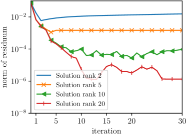
(c) Ga, Tucker, 3D, $\square$

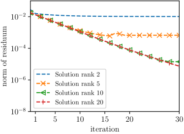
(d) GaNi, TT, 3D, $\mathrm{S}$

Although the truncation of the growing tensor’s rank can be provided by a tolerance to an approximation error, it is difficult to set up the parameters properly during the solver. Particularly it may happen that the rank significantly increase resulting in unnecessary computational demands, especially when the tensors are far away from the solution. Therefore the truncation has been performed to a fixed rank. The solution which is from a large dimensional space $\mathbb{R}^{\boldsymbol{N}}$ with the dimension $\prod_{\alpha=1}^{d}N_{\alpha}$ is approximated with a significantly smaller number of parameters. Therefore there is always a residual error which can be diminished only by an increasing rank of the low-rank formats. Note that the rank-one tensors occurring in all three low-rank formats are automatically computed by a solver and are thus suboptimal global basis vectors for the particular problem. Therefore the method can be seen as a model order reduction technique.

From the results in Figure 2.2.2, we can observe that solutions with higher rank have larger potential in reducing the norm of residuum regardless the discretisation method (Ga and GaNi), material problem ($\square$ and $\mathrm{S}$), or the low-rank format (CP, Tucker, TT). This proposes a rank adapting solver that starts with a lower solution rank and increases the rank during the iterations. We also notice that the norms of residuum during iterations decrease with higher rate for the problem with the square inclusion (material $\square$), however, the rate is more stable for the material S. Although, the material $\square$ was systematically computed with GaNi method and material S with Ga, which is in accordance with the recommendation in [57], the discretisation method has no influence on the character of the behaviour during iterations. These finding are in agreement with [37] analysing the stochastic linear systems and solvers approximated with low-rank approximations.

Note that the computation of the Frobenius norm of tensors in Tucker format is computationally demanding. Therefore, we have used the equivalent Frobenius norm of the Tucker’s core, which can be computed much faster.

4.3 Algebraic error of the low-rank approximations

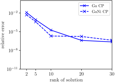
(a) 2D, $\square$

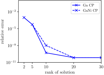
(b) 2D, $\mathrm{S}$

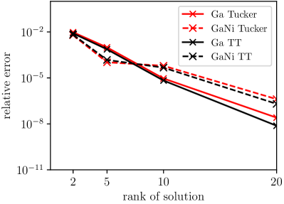
(c) 3D, $\square$

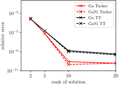
(d) 3D, $\mathrm{S}$

Figure 4: Relative errors (19) of low-rank solutions computed in 2D for $N=1215$ and in 3D for $N=135$.

In the Figure 4.3, the approximation properties of the low-rank formats are depicted. As an criterion, the relative algebraic error between the homogenised properties of low-rank solution $A_{\mathrm{H},{\boldsymbol{N}},r}$ and of the full solution $A_{\mathrm{H},{\boldsymbol{N}}}$ has been used, i.e.

$$\text{relative error}=\frac{A_{\mathrm{H},{\boldsymbol{N}}}-A_{\mathrm{H},{\boldsymbol{N}},r}}{A_{\mathrm{H},{\boldsymbol{N}}}}.$$ (19)

This is chosen because the error in the homogenised properties corresponds to the square of the energetic semi-norm (norm on zero-mean fields) of the algebraic error between the full solution and the low-rank approximation

$$\|u_{\boldsymbol{N}}-u_{{\boldsymbol{N}},r}\|_{A}^{2}=a\bigl{(}\nabla u_{\boldsymbol{N}}-\nabla u_{{\boldsymbol{N}},r},\nabla u_{\boldsymbol{N}}-\nabla u_{{\boldsymbol{N}},r}\bigr{)}=A_{\mathrm{H},{\boldsymbol{N}},r}-A_{\mathrm{H},{\boldsymbol{N}}}$$

for the derivation see [57, Appendix D]. We also note that the full solution $u_{\boldsymbol{N}}$ has been computed using conjugate gradients with high accuracy (tolerance $10^{-8}$ on the norm of the residuum) to obtain a solution that is close to the exact one. The low-rank solution has been obtained from minimal residual iteration, which was stopped when the residuum failed to be decreased. The minimal residual iteration was used to provide low-rank solution with the minimal norm of residuum.

We can observe that the results are again similar regardless of the discretisation method (Ga and GaNi), material problem ($\square$ and $\mathrm{S}$), or the low-rank format (CP, Tucker, TT). An increase in the solution rank leads to a significant reduction of the relative error. However, the low-rank approximations of the material S reach the threshold error corresponding to the full approximate solution obtained from the conjugate gradients. It also shows that the low-rank method is more accurate for a problem with continuous material property (material $\mathrm{S}$) than for the one with discontinuous coefficients (material $\square$).

4.4 Memory and computational efficiencies

	Element-wise product	FFTd	Truncation
full	$N^{d}$	$\mathcal{O}(N^{d}\log N$ )	—
CP	$dNrs$	$\mathcal{O}(dNr\log N)$	$\mathcal{O}(dNr^{2})$
Tucker	$dNrs+r^{d}s^{d}$	$\mathcal{O}(dNr\log N)$	$\mathcal{O}(dNr^{2}+r^{d+1})$
TT	$dNr^{2}s^{2}$	$\mathcal{O}(dNr^{2}\log N)$	$\mathcal{O}(dNr^{3})$

Table 2: Asymptotic computational complexities in terms of floating point multiplications. The operations are performed on full tensors of order $d$ and shape $(N,\dotsc,N)$, and on the same tensors in their CP, Tucker, and tensor-train (TT) formats with maximum rank $r$ and $s$ ($s$ for the second operand in a binary operation).

format	memory requirements
full	$N^{d}$
CP	$dNr$
Tucker	$dNr+r^{d}$
TT	$2Nr+(d-2)Nr^{2}$

Table 3: Memory requirements to store tensors of order $d$ with shape $(N,\dotsc,N)$ for full, CP, Tucker, and tensor-train (TT) formats with maximum rank $r$.

Here, we discuss the computational and memory requirements to resolve the linear system using low-rank approximations. Additionally to the previous examples, the CPU times and approximation properties of low-rank formats were tested for an anisotropic material. The heterogeneous material coefficients $\boldsymbol{A}_{\square}$ and $\boldsymbol{A}_{\mathrm{S}}$ were modified by adding a spatially constant anisotropic material tensor $\boldsymbol{B}$, i.e.

$$\widetilde{\boldsymbol{A}}_{\bullet}(\boldsymbol{x})=\boldsymbol{A}_{\bullet}(\boldsymbol{x})+\boldsymbol{B},$$

where the matrices

$$\boldsymbol{B} =\begin{pmatrix}5.5&-4.5\\ -4.5&5.5\end{pmatrix}, \boldsymbol{B} =\begin{pmatrix}4.25&-3.25&-1.25\sqrt{2}\\ -3.25&4.25&1.25\sqrt{2}\\ -1.25\sqrt{2}&1.25\sqrt{2}&7.5\end{pmatrix}$$

have eigenvalues $(1,10)$ in 2D and $(1,5,10)$ in 3D.

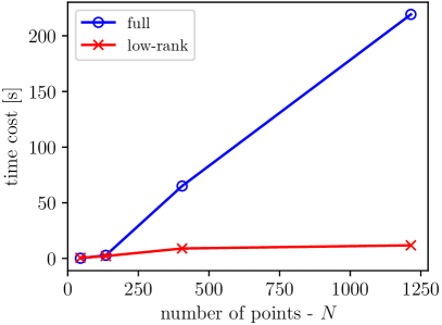
(a) 2D, $\square$, isotropic

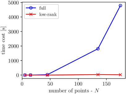
(b) 3D, $\square$, isotropic

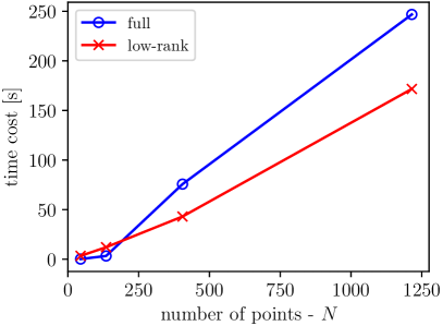
(c) 2D, $\square$, anisotropic

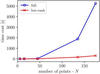
(d) 3D, $\square$, anisotropic

Figure 5: The CPU time of Ga solver to solve the problem with isotropic (1st row) and anisotropic (2nd row) material $\square$. The full solution has been computed on a grid of size $(N,\dotsc,N)$ while the low-rank solution on the grid $(3N,\dotsc,3N)$ with various solution ranks to achieve the same level of accuracy as the full scheme. The stopping criterion of conjugate gradients for the full solver was set to $10^{-6}$ on the norm of residuum.

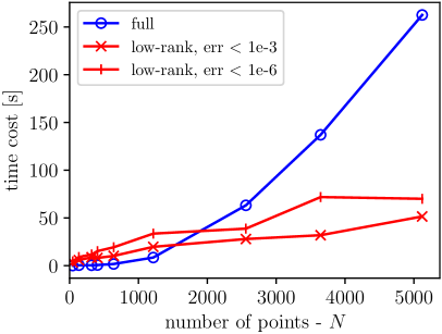
(a) 2D, S, isotropic

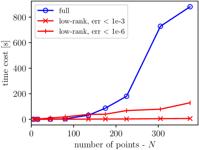
(b) 3D, S, isotropic

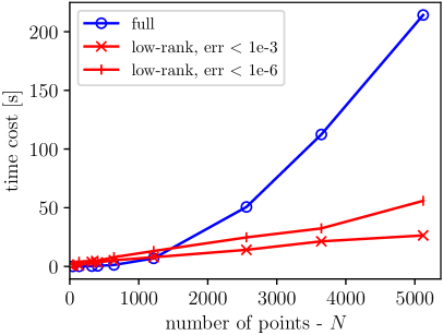
(c) 2D, S, anisotropic

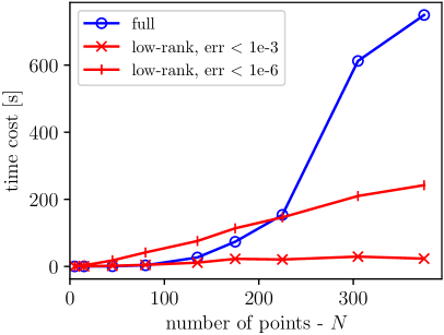
(d) 3D, S, anisotropic

Figure 6: The CPU time of GaNi solver to solve the problem with isotropic (1st row) and anisotropic (2nd row) material S. Both the full and low-rank solution are computed on the same grid. The stopping criterion of conjugate gradients for the full solver was set to $10^{-6}$ on the norm of residuum. The minimal residuum iteration for the low-rank approximation was computed with various rank to achieve a required error tolerance defined in (19).

	2D, $\square$				3D, $\square$
$N$	45	135	405	1215	5	15	45	135	175
$r$ (isotropic)	3	3	5	7	3	3	3	5	5
$r$ (anisotropic)	5	11	21	31	3	3	5	11	11

Table 4: Rank $r$ of low-rank solutions that reach the same accuracy as the full solution for various values of $N$, for isotropic and anisotropic material $\square$. The full solver has been computed with grid size $(N,\dotsc,N)$ while sparse solver with $(3N,\dotsc,3N)$. The stopping criterion of conjugate gradients for the full solver was set to $10^{-6}$ on the norm of residuum.

As we are using several low-rank formats and several operations on them, the computational complexities and memory requirements are summarised in Tables 2 and 3. The memory requirements of the FFT-based systems are controlled by memory requirements for material coefficients, preconditioner, solution vector, and possibly other vectors needed to store as a requirement of the linear solver. Provided that the ranks are kept small, the memory of low-rank solvers scales linearly with $N$, while full solver scales with $N^{d}$, which makes the method effective particularly for tensor with high order.

We compare the CPU time of full and low-rank solvers for homogenisation with exact integration (Ga) on the same level of accuracy measured by the energetic norm. It is achieved by the following procedure. The reference full solution was computed using conjugate gradient method on the regular grid $(N,\dotsc,N)$ with the tolerance $10^{-6}$ on the norms of residua. In order to achieve the same accuracy as the full solution, the low-rank solver was run on a bigger grid $(\alpha N,\dotsc,\alpha N)$ with the multiplier $\alpha=3$. The rank of low-rank approximations was increased step-by-step until it achieved a required error tolerance defined in (19). The iterations of the low-rank solver (for a given rank) are stopped when the residuum fails to decrease. This procedure, which creates a great possibility for a rank reduction in the low-rank solution, is applicable only for problems that allow an exact integration of material coefficients (here material $\square$).

The results in Figure 5 shows that the CPU time scales as $N^{d}$ for a full solution, and almost linearly for low-rank solutions on the isotropic material $\square$. In the anisotropic cases the time costs of low-rank solutions are relatively higher but still cheaper than that of the full solution. The difference in these two cases is due to the different ranks of the low-rank solutions. For isotropic material $\square$, the solution rank increases only slowly with $N$ , while for its anisotropic counterpart the rank increases at a faster rate (as tabulated in the Table 4). In general, the results show that the low-rank solver are significantly faster for larger $N$, despite being run on a larger computational grid.

We also did the comparison of both solvers for the isotropic and anisotropic material S. However, the smooth material S is better suited for the homogenisation with the numerical integration (GaNi), see the comparison in [57]. Therefore, the comparison of the solvers is run on the same discretisation grid. The ranks of the low-rank solution are chosen such that it achieves a relative error (as defined in (19)) below $10^{-3}$ or $10^{-6}$. The ranks remain stable when $N$ increases, which makes the CPU time of the low-rank solver almost linear in $N$, as shown in Figure 6.

5 Conclusion

This paper is focused on the acceleration of Fourier–Galerkin methods using low-rank tensor approximations for spatially $2$-dimensional and $3$-dimensional problems of numerical homogenisation. The efficiency of this approach builds on incorporation of the fast Fourier transform (FFT) and low-rank tensor approximation into the iterative linear solvers. The computational complexity is reduced to be quasilinear in the size of the discretisation and linear in spatial dimension $d$, since on a low-rank tensor of order $d$, the $d$-dimensional FFT can be performed as a series of one-dimensional FFTs. In this paper three formats — canonical polyadic (CP), Tucker, and tensor train (TT) — have been considered, and all of them show similar advantage in saving the computational cost.

The main results are summarised as the following:

• The incorporation of low-rank tensor approximations lead to a significant reduction of memory and computational cost in the solution of the homogenisation problems.

• The method is more suitable for material coefficients with relatively smaller rank. The low-rank approximation solvers computationally benefits from the better asymptotic behaviour, see Table 2 and 3. The advantage is accentuated for problems of a higher spatial dimension $d$ leading to tensors with order $d$.

• The low-rank approximation can be seen as a model order reduction technique.

Since the low-rank approximation provides a significant memory reduction it allows to compute the solution on a finer grid. Therefore, the proposed method based on low-rank approximation may provide more accurate solution than the conventional method based on full tensors, especially when the material is of a relatively small rank.

Appendix A Low-rank tensor approximations

Here we provide more details of the low-rank tensor approximations techniques utilized in this paper. This includes the approximation in CP, Tucker and tensor train formats.

A.1 The canonical polyadic format

A canonical polyadic (CP) or $r$-term representation $\boldsymbol{\mathsfit{v}}_{r}$ of a tensor $\boldsymbol{\mathsfit{v}}\in\mathbb{K}^{N_{1}\times\cdots\times N_{d}}$ ( $\mathbb{K}$ is either $\mathbb{R}$ or $\mathbb{C}$) is a sum of $r$ rank-$1$ tensors, i.e.

$$\boldsymbol{\mathsfit{v}}\approx\boldsymbol{\mathsfit{v}}_{r}=\sum^{r}_{i=1}\mathsfit{c}[i]\bigotimes^{d}_{j=1}\boldsymbol{\mathsfit{b}}^{(j)}[i]$$ (20)

with $\boldsymbol{\mathsfit{b}}^{(j)}\in\mathbb{K}^{r\times N_{j}}$ and $\bigotimes$ denotes tensor product. This format has linear storage size $r\sum^{d}_{j=1}N_{j}$. But for $d\geq 3$ and a given $r$, the construction of an error minimizing $\boldsymbol{\mathsfit{v}}_{r}$ is not always feasible [53, Proposition 9.10] because the space of CP format tensor with fixed $r$ is not closed [53, Lemma 9.11].

A.1.1 Element-wise multiplication

The element-wise (Hadamard) product of two tensors of ranks $r$ and $s$ in CP format is computed as:

$$\boldsymbol{\mathsfit{v}}_{r}\odot\boldsymbol{\mathsfit{w}}_{s}=\sum^{r}_{i=1}\sum^{s}_{k=1}\mathsfit{c}_{\boldsymbol{\mathsfit{v}}}[i]\mathsfit{c}_{\boldsymbol{\mathsfit{w}}}[k]\bigotimes^{d}_{j=1}\left(\boldsymbol{\mathsfit{b}}^{(j)}_{\boldsymbol{\mathsfit{v}}}[i]\odot\boldsymbol{\mathsfit{b}}^{(j)}_{\boldsymbol{\mathsfit{w}}}[k]\right).$$

This operation has complexity $rs\sum^{d}_{j=1}N_{j}$ and the product has a new rank $rs$.

A.1.2 Fourier transform

Due to the linearity and tensor structure of the Fourier transform $\mathcal{F}_{{\boldsymbol{N}}}$ of a size ${\boldsymbol{N}}\in\mathbb{N}^{d}$, a $d$-dimensional Fourier transform of a CP tensor is broken down to a series of $1$-d Fourier transform, i.e.,

$$\mathcal{F}_{{\boldsymbol{N}}}(\boldsymbol{\mathsfit{v}}_{r})=\sum^{r}_{i=1}\mathsfit{c}[i]\bigotimes^{d}_{j=1}\mathcal{F}_{N_{j}}(\boldsymbol{\mathsfit{b}}^{(j)}[i]).$$

Hence a FFT on a CP tensor has complexity $drN\log N$.

A.1.3 Rank truncation

Operations (e.g. element-wise multiplication) applied on tensors in CP format usually inflate the representation rank. This calls for a truncation to a prescribed rank or error tolerance.

For $d=2$, this reduction is done by rank truncation based on QR decomposition and singular value decomposition(SVD). Let the matrices $\boldsymbol{B}^{(j)}\in\mathbb{K}^{N_{j}\times r}$ collect the vectors $\{\boldsymbol{\mathsfit{b}}^{(j)}[i]\}^{r}_{i=1}$ for the $j$-th dimension, we have their re-orthogonalisations $\boldsymbol{B}^{(1)}=\boldsymbol{Q}^{(1)}\boldsymbol{R}^{(1)}$ and $\boldsymbol{B}^{(2)}=\boldsymbol{Q}^{(2)}\boldsymbol{R}^{(2)}$ by QR decompositions. A SVD $\boldsymbol{R}^{(1)}\boldsymbol{R}^{(2)}=\boldsymbol{U}^{(1)}\boldsymbol{\Sigma}(\boldsymbol{U}^{(2)})^{\top}$ facilitates the truncation. Suppose $\boldsymbol{U}^{(1)}_{k}$, $\boldsymbol{U}^{(2)}_{k}$ and $\boldsymbol{\Sigma}_{k}$ are the truncated ones with rank $k\leq r$, the truncated form of the CP representation (20) is

$$\boldsymbol{\mathsfit{v}}_{k}=\sum^{k}_{i=1}\mathsfit{c}[i]\widehat{\boldsymbol{\mathsfit{b}}}^{(1)}[i]\otimes\widehat{\boldsymbol{\mathsfit{b}}}^{(2)}[i]$$

where $\widehat{\boldsymbol{\mathsfit{b}}}^{(1)}[i]$, $\widehat{\boldsymbol{\mathsfit{b}}}^{(2)}[i]$ are the columns of $\boldsymbol{Q}^{(1)}\boldsymbol{U}^{(1)}_{k}$, $\boldsymbol{Q}^{(2)}\boldsymbol{U}^{(2)}_{k}$ respectively, and $\mathsfit{c}[i]$ are the diagonal entries of $\boldsymbol{\Sigma}_{k}$.

For $d\geq 3$, the $k$-rank form could be obtained by numerical error minimizing procedures [53], e.g. Alternative Least-Squares method. But there is no guarantee that the procedures would converge, and if they would, there is no guarantee that they converge to the global optimum. This is due to the non-closedness of the set of rank-$r$ CP tensors with $d\geq 3$.

A.2 Tucker format

A Tucker format representation (or tensor subspace representation) of a tensor $\boldsymbol{\mathsfit{v}}\in\mathbb{K}^{N_{1}\times\cdots\times N_{d}}\in\mathcal{V}$ is a linear combination of frames (usually orthogonal bases) of the tensor space $\mathcal{V}$. Suppose $\mathcal{V}=\bigotimes^{d}_{j=1}\mathcal{V}^{j}$, the subspace $\mathcal{V}^{j}$ has basis vectors $\{\boldsymbol{\mathsfit{b}}^{(j)}[i_{j}]\in\mathbb{K}^{N_{j}}:1\leq i_{j}\leq r_{j}\}$ with ranks $\boldsymbol{r}=(r_{1},\dotsc,r_{d})$. The tensors $\bigotimes^{d}_{j=1}\boldsymbol{\mathsfit{b}}^{(j)}[i_{j}]$ for all $1\leq i_{j}\leq r_{j}$ form the bases of the space $\mathcal{V}$. Then we have a unique coefficient $\mathsfit{c}[i_{1},i_{2},\dots,i_{d}]$ for every $\boldsymbol{\mathsfit{v}}\in\mathcal{V}$ such that

$$\boldsymbol{\mathsfit{v}}\approx\boldsymbol{\mathsfit{v}}_{\mathchoice{\displaystyle\boldsymbol{r}}{\textstyle\boldsymbol{r}}{\scriptstyle\boldsymbol{r}}{\scriptscriptstyle\boldsymbol{r}}}= \sum^{r_{1}}_{i_{1}=1}\cdots\sum^{r_{d}}_{i_{d}=1}\boldsymbol{\mathsfit{c}}_{\boldsymbol{\mathsfit{v}}}[i_{1},i_{2},\dots,i_{d}]\bigotimes^{d}_{j=1}\boldsymbol{\mathsfit{b}}^{(j)}_{\boldsymbol{\mathsfit{v}}}[i_{j}],$$ (21)

where $\boldsymbol{\mathsfit{c}}\in\mathbb{K}^{r_{1}\times\cdots\times r_{d}}$ is called the core tensor. Given any prescribed rank vector $\mathchoice{\displaystyle\boldsymbol{r}}{\textstyle\boldsymbol{r}}{\scriptstyle\boldsymbol{r}}{\scriptscriptstyle\boldsymbol{r}}$, an error minimizing approximation $\boldsymbol{\mathsfit{v}}_{\mathchoice{\displaystyle\boldsymbol{r}}{\textstyle\boldsymbol{r}}{\scriptstyle\boldsymbol{r}}{\scriptscriptstyle\boldsymbol{r}}}$ can be found by a high-order singular value decomposition (HOSVD) [58]. When the vectors $\{\boldsymbol{\mathsfit{b}}^{(j)}[i_{j}]\in\mathbb{K}^{N_{j}}:1\leq i_{j}\leq r_{j}\}$ form only a frame of the subspace $\mathcal{V}$ (e.g. after addition of two tensors), the core tensor is not unique, however, a representation with orthogonal bases can be obtained by applying QR decomposition to the frames and HOSVD to the accordingly updated core.

A.2.1 Element-wise multiplication

Let another Tucker format tensor with rank $\mathchoice{\displaystyle\boldsymbol{s}}{\textstyle\boldsymbol{s}}{\scriptstyle\boldsymbol{s}}{\scriptscriptstyle\boldsymbol{s}}$ be defined as

$$\boldsymbol{\mathsfit{w}}_{\mathchoice{\displaystyle\boldsymbol{s}}{\textstyle\boldsymbol{s}}{\scriptstyle\boldsymbol{s}}{\scriptscriptstyle\boldsymbol{s}}}=\sum^{\mathchoice{\displaystyle\boldsymbol{s}}{\textstyle\boldsymbol{s}}{\scriptstyle\boldsymbol{s}}{\scriptscriptstyle\boldsymbol{s}}}_{\mathchoice{\displaystyle\boldsymbol{k}}{\textstyle\boldsymbol{k}}{\scriptstyle\boldsymbol{k}}{\scriptscriptstyle\boldsymbol{k}}}\boldsymbol{\mathsfit{c}}_{\boldsymbol{\mathsfit{w}}}[\mathchoice{\displaystyle\boldsymbol{k}}{\textstyle\boldsymbol{k}}{\scriptstyle\boldsymbol{k}}{\scriptscriptstyle\boldsymbol{k}}]\bigotimes^{d}_{j=1}\boldsymbol{\mathsfit{b}}^{(j)}_{\boldsymbol{\mathsfit{w}}}[k_{j}]$$

the element-wise (Hadamard) product of $\boldsymbol{\mathsfit{v}}_{\mathchoice{\displaystyle\boldsymbol{r}}{\textstyle\boldsymbol{r}}{\scriptstyle\boldsymbol{r}}{\scriptscriptstyle\boldsymbol{r}}}$ and $\boldsymbol{\mathsfit{w}}_{\mathchoice{\displaystyle\boldsymbol{s}}{\textstyle\boldsymbol{s}}{\scriptstyle\boldsymbol{s}}{\scriptscriptstyle\boldsymbol{s}}}$ has also a Tucker format

$$\boldsymbol{\mathsfit{v}}_{\mathchoice{\displaystyle\boldsymbol{r}}{\textstyle\boldsymbol{r}}{\scriptstyle\boldsymbol{r}}{\scriptscriptstyle\boldsymbol{r}}}\odot\boldsymbol{\mathsfit{w}}_{\mathchoice{\displaystyle\boldsymbol{s}}{\textstyle\boldsymbol{s}}{\scriptstyle\boldsymbol{s}}{\scriptscriptstyle\boldsymbol{s}}}=\sum^{\mathchoice{\displaystyle\boldsymbol{t}}{\textstyle\boldsymbol{t}}{\scriptstyle\boldsymbol{t}}{\scriptscriptstyle\boldsymbol{t}}}_{\mathchoice{\displaystyle\boldsymbol{l}}{\textstyle\boldsymbol{l}}{\scriptstyle\boldsymbol{l}}{\scriptscriptstyle\boldsymbol{l}}}\boldsymbol{\mathsfit{c}}[\mathchoice{\displaystyle\boldsymbol{l}}{\textstyle\boldsymbol{l}}{\scriptstyle\boldsymbol{l}}{\scriptscriptstyle\boldsymbol{l}}]\bigotimes^{d}_{j=1}\boldsymbol{\mathsfit{b}}^{(j)}[l_{j}]$$

where $\mathchoice{\displaystyle\boldsymbol{t}}{\textstyle\boldsymbol{t}}{\scriptstyle\boldsymbol{t}}{\scriptscriptstyle\boldsymbol{t}}=\mathchoice{\displaystyle\boldsymbol{r}}{\textstyle\boldsymbol{r}}{\scriptstyle\boldsymbol{r}}{\scriptscriptstyle\boldsymbol{r}}\odot\mathchoice{\displaystyle\boldsymbol{s}}{\textstyle\boldsymbol{s}}{\scriptstyle\boldsymbol{s}}{\scriptscriptstyle\boldsymbol{s}}$ and $\boldsymbol{\mathsfit{c}}=\boldsymbol{\mathsfit{c}}_{\boldsymbol{\mathsfit{v}}}\otimes\boldsymbol{\mathsfit{c}}_{\boldsymbol{\mathsfit{w}}}$, i.e. the Kronecker product of the two coefficient tensors. So for any $1\leq j\leq d$, the index $l_{j}$ is related to $i_{j}$ and $k_{j}$ by $l_{j}=\overline{i_{j}k_{j}}=i_{j}r_{j}+k_{j}$, and $u$ is obtained from $v$ and $w$ through

$$u^{(j)}_{l_{j}}=u^{(j)}_{\overline{i_{j}k_{j}}}=v^{(j)}_{i_{j}}\odot w^{(j)}_{k_{j}}\mbox{\;\;\; for \;\; }1\leq i_{j}\leq r_{j},\;1\leq k_{j}\leq s_{j}$$

Let $N=\max_{i}N_{i}$, $r=\max_{i}r_{i}$ and $s=\max_{i}s_{i}$, the computational complexity of the element-wise product is bounded by $dNrs+r^{d}s^{d}$, in which the first term is the cost for computing $\{u^{(j)}_{l_{j}}:1\leq l_{j}\leq R_{j}\}_{j=1}^{d}$, and the second for the Kronecker product of coefficient tensors.

A.2.2 Fourier transform

The Fourier transform of $\boldsymbol{\mathsfit{v}}_{\mathchoice{\displaystyle\boldsymbol{r}}{\textstyle\boldsymbol{r}}{\scriptstyle\boldsymbol{r}}{\scriptscriptstyle\boldsymbol{r}}}$ is

$$\mathcal{F}_{{\boldsymbol{N}}}(\boldsymbol{\mathsfit{v}}_{\mathchoice{\displaystyle\boldsymbol{r}}{\textstyle\boldsymbol{r}}{\scriptstyle\boldsymbol{r}}{\scriptscriptstyle\boldsymbol{r}}})=\sum^{\mathchoice{\displaystyle\boldsymbol{r}}{\textstyle\boldsymbol{r}}{\scriptstyle\boldsymbol{r}}{\scriptscriptstyle\boldsymbol{r}}}_{\mathchoice{\displaystyle\boldsymbol{i}}{\textstyle\boldsymbol{i}}{\scriptstyle\boldsymbol{i}}{\scriptscriptstyle\boldsymbol{i}}}\boldsymbol{\mathsfit{c}}[\mathchoice{\displaystyle\boldsymbol{i}}{\textstyle\boldsymbol{i}}{\scriptstyle\boldsymbol{i}}{\scriptscriptstyle\boldsymbol{i}}]\bigotimes^{d}_{j=1}\mathcal{F}_{N_{j}}(\boldsymbol{\mathsfit{b}}^{(j)}[i_{j}])$$

which only involves the basis vectors. If FFT is applied, the complexity is of order $\mathcal{O}(drN\log N)$.

A.2.3 Rank truncation

The Tucker representation (21) can be obtained either by a HOSVD applied on a full tensor or by an operation (e.g. element-wise multiplication) over other Tucker operands. In the first case, an error minimizing rank truncation is readily available due to the property of HOSVD:

$$\sigma^{(j)}_{1}\geq\sigma^{(j)}_{2}\geq\cdots\geq\sigma^{(j)}_{r_{j}},\quad\mbox{for }j=1,\cdots,d,$$

where $\sigma^{(j)}_{i_{j}}$ is the $2$-norm of the $i_{j}$-th slice of the core tensor $\boldsymbol{\mathsfit{c}}$ cut on the $j$-th dimension. If the truncation rank is $k_{j}<r_{j}$, the error of the truncated representation $\boldsymbol{\mathsfit{v}}_{\mathchoice{\displaystyle\boldsymbol{k}}{\textstyle\boldsymbol{k}}{\scriptstyle\boldsymbol{k}}{\scriptscriptstyle\boldsymbol{k}}}$ is bounded by

$$\|{\boldsymbol{\mathsfit{v}}}_{\mathchoice{\displaystyle\boldsymbol{r}}{\textstyle\boldsymbol{r}}{\scriptstyle\boldsymbol{r}}{\scriptscriptstyle\boldsymbol{r}}}-{\boldsymbol{\mathsfit{v}}}_{\mathchoice{\displaystyle\boldsymbol{k}}{\textstyle\boldsymbol{k}}{\scriptstyle\boldsymbol{k}}{\scriptscriptstyle\boldsymbol{k}}}\|\leq\left[\sum^{d}_{j=1}\sum^{r_{j}}_{i=k_{j}+1}(\sigma^{(j)}_{i})^{2}\right]^{1/2}.$$

In the second case the bases $\{\boldsymbol{\mathsfit{b}}^{(j)}[i_{j}]\}^{r_{j}}_{i_{j}=1}$ have to be re-orthogonalised first, and then a HOSVD of the updated core tensor is to be made to facilitate the truncation as in the first case. This procedure [53, as detailed in] is analogues to the re-orthogonalisation and SVD for the 2D CP format representations, but with higher tensor order.

A.3 Tensor train format

A tensor train(TT) representation [39] of a tensor $\boldsymbol{\mathsfit{v}}\in\mathbb{K}^{N_{1}\times\cdots\times N_{d}}$ can be expressed as a series of consecutive contractions of tensors $\boldsymbol{\mathsfit{b}}^{(j)}\in\mathbb{K}^{r_{j-1}\times N_{j}\times r_{j}}$ of order $3$ for $j=1,\cdots,d$, which are the carriages of the tensor train. An equivalent expression in the form of tensor products is

$$\boldsymbol{\mathsfit{v}}\approx\boldsymbol{\mathsfit{v}}_{\mathchoice{\displaystyle\boldsymbol{r}}{\textstyle\boldsymbol{r}}{\scriptstyle\boldsymbol{r}}{\scriptscriptstyle\boldsymbol{r}}} =\sum^{r_{1}}_{i_{1}=1}\cdots\sum^{r_{d-1}}_{i_{d-1}=1}\boldsymbol{\mathsfit{b}}^{(1)}_{\boldsymbol{\mathsfit{v}}}[1,:,i_{1}]\otimes\boldsymbol{\mathsfit{b}}^{(2)}_{\boldsymbol{\mathsfit{v}}}[i_{1},:,i_{2}]\otimes\cdots\otimes\boldsymbol{\mathsfit{b}}^{(d)}_{\boldsymbol{\mathsfit{v}}}[i_{d-1},:,1]$$

$\mathchoice{\displaystyle\boldsymbol{r}}{\textstyle\boldsymbol{r}}{\scriptstyle\boldsymbol{r}}{\scriptscriptstyle\boldsymbol{r}}$ is the TT-rank of $\boldsymbol{\mathsfit{v}}$ with a constrain $r_{0}=r_{d}=1$ to keep the elements of $\boldsymbol{\mathsfit{v}}$ scalars. The TT format is stable in the sense that for any prescribed $\mathchoice{\displaystyle\boldsymbol{r}}{\textstyle\boldsymbol{r}}{\scriptstyle\boldsymbol{r}}{\scriptscriptstyle\boldsymbol{r}}$ an error minimizing $\boldsymbol{\mathsfit{v}}_{\mathchoice{\displaystyle\boldsymbol{r}}{\textstyle\boldsymbol{r}}{\scriptstyle\boldsymbol{r}}{\scriptscriptstyle\boldsymbol{r}}}$ can always be constructed by a series of SVDs on consecutive matricisations of $\boldsymbol{\mathsfit{v}}$.

A.3.1 Element-wise multiplication

Let another TT format tensor with rank $\mathchoice{\displaystyle\boldsymbol{s}}{\textstyle\boldsymbol{s}}{\scriptstyle\boldsymbol{s}}{\scriptscriptstyle\boldsymbol{s}}$ be defined as

$$\boldsymbol{\mathsfit{w}}_{\mathchoice{\displaystyle\boldsymbol{s}}{\textstyle\boldsymbol{s}}{\scriptstyle\boldsymbol{s}}{\scriptscriptstyle\boldsymbol{s}}}=\sum^{s_{1}}_{i_{1}=1}\cdots\sum^{s_{d-1}}_{i_{d-1}=1}\boldsymbol{\mathsfit{b}}^{(1)}_{\boldsymbol{\mathsfit{w}}}[1,:,i_{1}]\otimes\boldsymbol{\mathsfit{b}}^{(2)}_{\boldsymbol{\mathsfit{w}}}[i_{1},:,i_{2}]\otimes\cdots\otimes\boldsymbol{\mathsfit{b}}^{(d)}_{\boldsymbol{\mathsfit{w}}}[i_{d-1},:,1]$$

with $\boldsymbol{\mathsfit{b}}^{(j)}_{\boldsymbol{\mathsfit{w}}}\in\mathbb{K}^{s_{j-1}\times N_{j}\times s_{j}}$. The element-wise product of $\boldsymbol{\mathsfit{v}}_{\mathchoice{\displaystyle\boldsymbol{r}}{\textstyle\boldsymbol{r}}{\scriptstyle\boldsymbol{r}}{\scriptscriptstyle\boldsymbol{r}}}$ and $\boldsymbol{\mathsfit{w}}_{\mathchoice{\displaystyle\boldsymbol{s}}{\textstyle\boldsymbol{s}}{\scriptstyle\boldsymbol{s}}{\scriptscriptstyle\boldsymbol{s}}}$ can also be expressed in TT format:

$$\boldsymbol{\mathsfit{v}}_{\mathchoice{\displaystyle\boldsymbol{r}}{\textstyle\boldsymbol{r}}{\scriptstyle\boldsymbol{r}}{\scriptscriptstyle\boldsymbol{r}}}\odot\boldsymbol{\mathsfit{w}}_{\mathchoice{\displaystyle\boldsymbol{s}}{\textstyle\boldsymbol{s}}{\scriptstyle\boldsymbol{s}}{\scriptscriptstyle\boldsymbol{s}}}=\sum^{t_{1}}_{i_{1}=1}\cdots\sum^{t_{d-1}}_{i_{d-1}=1}\boldsymbol{\mathsfit{b}}^{(1)}[1,:,i_{1}]\otimes\boldsymbol{\mathsfit{b}}^{(2)}[i_{1},:,i_{2}]\otimes\cdots\otimes\boldsymbol{\mathsfit{b}}^{(d)}[i_{d-1},:,1]$$

where $\mathchoice{\displaystyle\boldsymbol{t}}{\textstyle\boldsymbol{t}}{\scriptstyle\boldsymbol{t}}{\scriptscriptstyle\boldsymbol{t}}=\mathchoice{\displaystyle\boldsymbol{r}}{\textstyle\boldsymbol{r}}{\scriptstyle\boldsymbol{r}}{\scriptscriptstyle\boldsymbol{r}}\odot\mathchoice{\displaystyle\boldsymbol{s}}{\textstyle\boldsymbol{s}}{\scriptstyle\boldsymbol{s}}{\scriptscriptstyle\boldsymbol{s}}$ and $\boldsymbol{\mathsfit{b}}^{(j)}=\boldsymbol{\mathsfit{b}}^{(j)}_{\boldsymbol{\mathsfit{v}}}\ast\boldsymbol{\mathsfit{b}}^{(j)}_{\boldsymbol{\mathsfit{w}}}$. Here the $\ast$ denotes one type of Khatri–Rao product [59] which makes Kronecker product only in the first and third dimensions, i.e. it yields an order $3$ tensor $\boldsymbol{\mathsfit{b}}^{(j)}\in\mathbb{K}^{r_{j-1}s_{j-1}\times N_{j}\times r_{j}s_{j}}$. The complexity of the element-wise product is of order $\mathcal{O}(dNr^{2}s^{2})$ with $N$, $r$ and $s$ as defined in the subsection A.2.

A.3.2 Fourier transform

The Fourier transform of $\boldsymbol{\mathsfit{v}}_{\mathchoice{\displaystyle\boldsymbol{r}}{\textstyle\boldsymbol{r}}{\scriptstyle\boldsymbol{r}}{\scriptscriptstyle\boldsymbol{r}}}$ can also be carried out by doing $1$-D transforms on each carriage:

$$\mathcal{F}_{{\boldsymbol{N}}}(\boldsymbol{\mathsfit{v}}_{\mathchoice{\displaystyle\boldsymbol{r}}{\textstyle\boldsymbol{r}}{\scriptstyle\boldsymbol{r}}{\scriptscriptstyle\boldsymbol{r}}})=\sum^{r_{1}}_{i_{1}=1}\cdots\sum^{r_{d-1}}_{i_{d-1}=1}\mathcal{F}_{N_{1}}(\boldsymbol{\mathsfit{b}}^{(1)}_{\boldsymbol{\mathsfit{v}}}[1,:,i_{1}])\otimes\mathcal{F}_{N_{2}}(\boldsymbol{\mathsfit{b}}^{(2)}_{\boldsymbol{\mathsfit{v}}}[i_{1},:,i_{2}])\otimes\cdots\otimes\mathcal{F}_{N_{d}}(\boldsymbol{\mathsfit{b}}^{(d)}_{\boldsymbol{\mathsfit{v}}}[i_{d-1},:,1])$$

in which the $\mathcal{F}_{N_{j}}(\cdot)$ is made on the fibres along the second mode. If FFT is applied here, the number of operations is of order $\mathcal{O}(dr^{2}N\log N)$.

A.3.3 Rank truncation

The tensor train representation (LABEL:eq:TT) can be obtained either by transforming a full tensor into tensor train format by using $d-1$ sequential SVDs applied on auxiliary matrices of the tensor (known as TT-SVD) [39], or as a result of operations (e.g. additions or multiplications) over tensor train operands. In the first case, an error minimising rank truncation could be directly carried out in the TT-SVD process. The truncation has an error bound $(\sum^{d-1}_{k=1}\epsilon^{2}_{k})^{1/2}$, where $\epsilon_{k}$ is the Frobenious norm error introduced by the truncation of the $k$-th SVD. In the second case, a re-orthogonalisation has to be done in the first place, this is followed by $d-1$ sequential SVDs on unfolded carriages. This process is known as TT-truncation (also called rounding).

For the first case, the complexity of truncation is the same as that for the TT-SVD, which is of order $\mathcal{O}(N^{d+1})$. A cheaper alternative for TT-SVD is TT-cross approximation as introduced in [38]. The complexity of TT-truncation in the second case is of order $\mathcal{O}(dNr^{3})$.

Acknowledgements

Funded by the Deutsche Forschungsgemeinschaft (DFG, German Research Foundation) — project number MA2236/27-1.

Martin Ladecký was supported by the Czech Science Foundation through projects No. GAČR 17-04150J, by the Center of Advanced Applied Sciences (CAAS), financially supported by the European Regional Development Fund (through project No. CZ.02.1.01/0.0/0.0/16_019/0000778), and by the Grant Agency of the CTU in Prague, grant No. SGS19/002/OHK1/1T/11.

References

- [1] H. Moulinec, P. Suquet, A fast numerical method for computing the linear and nonlinear mechanical properties of composites, Comptes rendus de l’Académie des sciences. Série II, Mécanique, physique, chimie, astronomie 318 (11) (1994) 1417–1423.
- [2] J. Vondřejc, J. Zeman, I. Marek, An FFT-based Galerkin method for homogenization of periodic media, Computers & Mathematics with Applications 68 (3) (2014) 156–173. doi:10.1016/j.camwa.2014.05.014.
- [3] G. W. Milton, The Theory of Composites, Cambridge Monographs on Applied and Computational Mathematics, Cambridge University Press, Cambridge, UK, 2002.
- [4] J. Zeman, T. W. J. de Geus, J. Vondřejc, R. H. J. Peerlings, M. G. D. Geers, A finite element perspective on non-linear FFT-based micromechanical simulations, International Journal for Numerical Methods in Engineering 111 (10) (2017) 903–926. doi:10.1002/nme.5481.
- [5] T. W. J. de Geus, J. Vondřejc, J. Zeman, R. H. J. Peerlings, M. G. D. Geers, Finite strain FFT-based non-linear solvers made simple, Computer Methods in Applied Mechanics and Engineering 318 (2017) 412–430. doi:10.1016/j.cma.2016.12.032.
- [6] J. Vondřejc, J. Zeman, I. Marek, Guaranteed upper-lower bounds on homogenized properties by FFT-based Galerkin method, Computer Methods in Applied Mechanics and Engineering 297 (2015) 258–291. doi:10.1016/j.cma.2015.09.003.
- [7] J. Zeman, J. Vondřejc, J. Novák, I. Marek, Accelerating a FFT-based solver for numerical homogenization of periodic media by conjugate gradients, Journal of Computational Physics 229 (21) (2010) 8065–8071. doi:10.1016/j.jcp.2010.07.010.
- [8] J. Vondřejc, Improved guaranteed computable bounds on homogenized properties of periodic media by the Fourier–Galerkin method with exact integration, International Journal for Numerical Methods in Engineering 107 (13) (2016) 1106–1135. doi:10.1002/nme.5199.
- [9] M. Schneider, Convergence of FFT-based homogenization for strongly heterogeneous media, Mathematical Methods in the Applied Sciences 38 (13) (2014) 2761–2778. doi:10.1002/mma.3259.
- [10] S. Brisard, L. Dormieux, Combining Galerkin approximation techniques with the principle of Hashin and Shtrikman to derive a new FFT-based numerical method for the homogenization of composites, Computer Methods in Applied Mechanics and Engineering 217–220 (2012) 197–212. doi:10.1016/j.cma.2012.01.003.
- [11] S. Brisard, L. Dormieux, FFT-based methods for the mechanics of composites: A general variational framework, Computational Materials Science 49 (3) (2010) 663–671. doi:doi:10.1016/j.commatsci.2010.06.009.
- [12] M. Schneider, D. Merkert, M. Kabel, FFT-based homogenization for microstructures discretized by linear hexahedral elements, International Journal for Numerical Methods in Engineering 109 (10) (2017) 1461–1489. doi:10.1002/nme.5336.
- [13] F. Willot, Fourier-based schemes for computing the mechanical response of composites with accurate local fields, Comptes Rendus Mécanique 343 (2015) 232–245. doi:10.1016/j.crme.2014.12.005.
- [14] F. Willot, B. Abdallah, Y.-P. Pellegrini, Fourier-based schemes with modified Green operator for computing the electrical response of heterogeneous media with accurate local fields, International Journal for Numerical Methods in Engineering 98 (7) (2014) 518–533. doi:10.1002/nme.4641.
- [15] D. J. Eyre, G. W. Milton, A fast numerical scheme for computing the response of composites using grid refinement, The European Physical Journal Applied Physics 6 (1) (1999) 41–47.
- [16] H. Moulinec, P. Suquet, G. W. Milton, Convergence of iterative methods based on Neumann series for composite materials: Theory and practice, International Journal for Numerical Methods in Engineering 114 (10) (2018) 1103–1130. doi:10.1002/nme.5777.
- [17] N. Mishra, J. Vondřejc, J. Zeman, A comparative study on low-memory iterative solvers for FFT-based homogenization of periodic media, Journal of Computational Physics 321 (2016) 151–168. doi:10.1016/j.jcp.2016.05.041.
- [18] M. Kabel, T. Böhlke, M. Schneider, Efficient fixed point and Newton–Krylov solvers for FFT-based homogenization of elasticity at large deformations, Computational Mechanics 54 (6) (2014) 1497–1514. doi:10.1007/s00466-014-1071-8.
- [19] M. Schneider, An FFT-based fast gradient method for elastic and inelastic unit cell homogenization problems, Computer Methods in Applied Mechanics and Engineering 315 (2017) 846–866. doi:10.1016/j.cma.2016.11.004.
- [20] J. Kochmann, B. Svendsen, S. Reese, L. Ehle, S. Wulfinghoff, J. Mayer, Efficient and accurate two-scale FE-FFT-based prediction of the effective material behavior of elasto-viscoplastic polycrystals, Computational Mechanics 61 (6) (2017) 751–764. doi:10.1007/s00466-017-1476-2.
- [21] F. S. Göküzüm, M. A. Keip, An algorithmically consistent macroscopic tangent operator for FFT-based computational homogenization, International Journal for Numerical Methods in Engineering 113 (4) (2018) 581–600. doi:10.1002/nme.5627.
- [22] F. Dietrich, D. Merkert, B. Simeon, Derivation of higher-order terms in FFT-based numerical homogenization, in: Lecture Notes in Computational Science and Engineering, Vol. 126, 2019, pp. 289–297. doi:10.1007/978-3-319-96415-7_25.
- [23] N. Bertin, L. Capolungo, A FFT-based formulation for discrete dislocation dynamics in heterogeneous media, Journal of Computational Physics 355 (2018) 366–384. doi:10.1016/J.JCP.2017.11.020.
- [24] T. W. J. de Geus, R. H. J. Peerlings, M. G. D. Geers, Competing damage mechanisms in a two-phase microstructure: How microstructure and loading conditions determine the onset of fracture, International Journal of Solids and Structures 97 (2016) 687–698. doi:10.1016/j.ijsolstr.2016.03.029.
- [25] M. Boeff, F. Gutknecht, P. S. Engels, A. Ma, A. Hartmaier, Formulation of nonlocal damage models based on spectral methods for application to complex microstructures, Engineering Fracture Mechanics 147 (2015) 373–387. doi:10.1016/j.engfracmech.2015.06.030.
- [26] J. Segurado, R. A. Lebensohn, J. Llorca, Computational Homogenization of Polycrystals, Advances in Applied Mechanics 51 (2018) 1–114. doi:10.1016/bs.aams.2018.07.001.
- [27] C. Garcia-Cardona, R. Lebensohn, M. Anghel, Parameter estimation in a thermoelastic composite problem via adjoint formulation and model reduction, International Journal for Numerical Methods in Engineering 112 (6) (2017) 578–600. doi:10.1002/nme.5530.
- [28] S. A. Goreinov, E. E. Tyrtyshnikov, N. L. Zamarashkin, A theory of pseudoskeleton approximations, Linear Algebra and Its Applications 261 (1-3) (1997) 1–21. doi:10.1016/S0024-3795(96)00301-1.
- [29] M. Bebendorf, Approximation of boundary element matrices, Numerische Mathematik 86 (4) (2000) 565–589. doi:10.1007/PL00005410.
- [30] W. Hackbusch, Numerical tensor calculus, Acta numerica 23 (2014) 651–742. doi:10.1017/S0962492914000087.
- [31] T. G. Kolda, B. W. Bader, Tensor Decompositions and Applications, SIAM Review 51 (3) (2009) 455–500. doi:10.1137/07070111X.
- [32] L. Giraldi, A. Nouy, G. Legrain, P. Cartraud, Tensor-based methods for numerical homogenization from high-resolution images, Computer Methods in Applied Mechanics and Engineering 254 (2013) 154–169. doi:10.1016/j.cma.2012.10.012.
- [33] D. Kressner, C. Tobler, Low-Rank Tensor Krylov Subspace Methods for Parametrized Linear Systems, SIAM Journal on Matrix Analysis and Applications 32 (4) (2011) 1288–1316. doi:10.1137/100799010.
- [34] C. Tobler, Low-rank tensor methods for linear systems and eigenvalue problems, Ph.D. thesis, ETH Zürich (2012).
- [35] S. V. Dolgov, TT-GMRES: Solution to a linear system in the structured tensor format, Russian Journal of Numerical Analysis and Mathematical Modelling 28 (2) (2013) 149–172. doi:10.1515/rnam-2013-0009.
- [36] J. Ballani, L. Grasedyck, A projection method to solve linear systems in tensor format, Numerical Linear Algebra with Applications 20 (1) (2013) 27–43. doi:10.1002/nla.1818.
- [37] H. G. Matthies, E. Zander, Solving stochastic systems with low-rank tensor compression, Linear Algebra and its Applications 436 (10) (2012) 3819–3838. doi:10.1016/j.laa.2011.04.017.
- [38] I. Oseledets, E. Tyrtyshnikov, TT-cross approximation for multidimensional arrays, Linear Algebra and its Applications 432 (1) (2010) 70–88. doi:10.1016/J.LAA.2009.07.024.
- [39] I. V. Oseledets, Tensor-Train Decomposition, SIAM Journal on Scientific Computing 33 (5) (2011) 2295–2317. doi:10.1137/090752286.
- [40] D. Bigoni, A. P. Engsig-Karup, Y. M. Marzouk, Spectral Tensor-Train Decomposition, SIAM Journal on Scientific Computing 38 (4) (2016) A2405–A2439. doi:10.1137/15M1036919.
- [41] M. Espig, W. Hackbusch, A. Litvinenko, H. G. Matthies, P. Wähnert, Efficient low-rank approximation of the stochastic Galerkin matrix in tensor formats, Computers & Mathematics with Applications 67 (4) (2014) 818–829. doi:10.1016/j.camwa.2012.10.008.
- [42] A. Nouy, Low-rank methods for high-dimensional approximation and model order reduction, in: Model Reduction and Approximation: Theory and Algorithms, Society for Industrial and Applied Mathematics, 2015, pp. 1–73. doi:10.1007/978-3-319-11259-6_21-1.
- [43] B. N. Khoromskij, C. Schwab, Tensor-Structured Galerkin Approximation of Parametric and Stochastic Elliptic PDEs, SIAM Journal on Scientific Computing 33 (1) (2011) 364–385. doi:10.1137/100785715.
- [44] B. N. Khoromskij, S. I. Repin, A fast iteration method for solving elliptic problems with quasiperiodic coefficients, Russian Journal of Numerical Analysis and Mathematical Modelling 30 (6) (2015) 329–344. doi:10.1515/rnam-2015-0030.
- [45] B. Khoromskij, S. Repin, Rank Structured Approximation Method for Quasi-Periodic Elliptic Problems, Computational Methods in Applied Mathematics 17 (3) (2017) 457–477. doi:10.1515/cmam-2017-0014.
- [46] A. Nouy, Low-Rank Tensor Methods for Model Order Reduction, in: Handbook of Uncertainty Quantification, Springer International Publishing, Cham, 2015, pp. 1–26. doi:10.1007/978-3-319-11259-6_21-1.
- [47] J. Kochmann, K. Manjunatha, C. Gierden, S. Wulfinghoff, B. Svendsen, S. Reese, A simple and flexible model order reduction method for FFT-based homogenization problems using a sparse sampling technique, Computer Methods in Applied Mechanics and Engineering 347 (2019) 622–638. doi:10.1016/j.cma.2018.11.032.
- [48] A. Bensoussan, J.-L. Lions, G. Papanicolaou, Asymptotic Analysis for Periodic Structures, North Holland, Amsterdam, 1978.
- [49] J. Saranen, G. Vainikko, Periodic Integral and Pseudodifferential Equations with Numerical Approximation, Springer Monographs Mathematics, Berlin, Heidelberg, 2002.
- [50] H. Moulinec, P. Suquet, A numerical method for computing the overall response of nonlinear composites with complex microstructure, Computer Methods in Applied Mechanics and Engineering 157 (1–2) (1998) 69–94. doi:10.1016/S0045-7825(97)00218-1.
- [51] J. Vondřejc, Double-grid quadrature with interpolation-projection (DoGIP) as a novel discretisation approach: An application to FEM on simplexes, Computers & Mathematics with Applications 78 (11) (2019) 3501–3513. doi:10.1016/j.camwa.2019.05.021.
- [52] M. Ladecký, I. Pultarová, J. Vondřejc, J. Zeman, Preconditioning the spectral Fourier method for homogenization of periodic media (2019).
- [53] W. Hackbusch, Tensor Spaces and Numerical Tensor Calculus, Springer Science & Business Media, Berlin, Heidelberg, 2012. doi:10.1007/978-3-540-78862-1.
- [54] Y. Saad, Iterative Methods for Sparse Linear Systems, 2nd Edition, SIAM, Philadelphia, PA, USA, 2003.
- [55] R. J. Adler, J. E. Taylor, Random fields and geometry, Springer, New York, 2009.
- [56] B. Matérn, Spatial Variation, Vol. 36 of Lecture Notes in Statistics, Springer New York, New York, NY, 1986. doi:10.1007/978-1-4615-7892-5.
- [57] J. Vondřejc, T. W. J. de Geus, Energy-based comparison between the Fourier–Galerkin method and the finite element method, Journal of Computational and Applied Mathematics 374 (2020) 112585. doi:10.1016/j.cam.2019.112585.
- [58] L. De Lathauwer, B. De Moor, J. Vandewalle, A Multilinear Singular Value Decomposition, SIAM Journal on Matrix Analysis and Applications 21 (4) (2000) 1253–1278. doi:10.1137/S0895479896305696.
- [59] C. G. Khatri, C. R. Rao, Solutions to Some Functional Equations and Their Applications to Characterization of Probability Distributions, Sankhyā: The Indian Journal of Statistics, Series A 30 (2) (1968) 167–180. doi:10.2307/25049527.