Eliciting ambiguity with mixing bets

Abstract

I show how to reveal ambiguity-sensitive preferences over a single natural event. In the proposed elicitation mechanism, agents mix binarized bets on the uncertain event and its complement under varying betting odds. The mechanism identifies the interval of relevant probabilities for maxmin and maxmax preferences. For variational preferences and smooth second-order preferences, the mechanism reveals inner bounds, that are sharp under high stakes. For small stakes, mixing under second-order preferences is dominated by the variance of the second-order distribution. Additionally, the mechanism can distinguish extreme ambiguity aversion as in maxmin preferences and moderate ambiguity aversion as in variational or smooth second-order preferences. An experimental implementation suggests that participants perceive almost as much ambiguity for the stock index and actions of other participants as for the Ellsberg urn, indicating the importance of ambiguity in real-world decision-making.

Keywords— ambiguity aversion, binarized score, belief elicitation, revealed preferences, uncertainty aversion
JEL codes: D81, D82, D83.

1 Introduction

Most economic modeling is based on subjective expected utility (SEU) [52]. However, uncertainty often cannot be represented by a precise probability measure. Instead, the perception of uncertainty is ambiguous [39]. Initiated by [20], various experiments showed that ambiguity matters for decision making.

While artificially generated ambiguity in experiments is well studied, there is little evidence on ambiguity for natural uncertainty [6], which complicates real-world applications of ambiguity-sensitive preferences. In this paper, I propose a simple mechanism - mixing bets - that reveals subjective ambiguity for a natural event.

1.1 Separation of Ambiguity Perception: The Belief Interval

To understand the empirical content of decision models, it is crucial to separate perception and attitude [46]. This is especially important for decisions under ambiguity, where no rational benchmark exists. The large number and flexibility of ambiguity-sensitive preferences makes this separation challenging [21, 37, see the discussion in]. Following [38], ambiguity perception can be represented by the set of probabilities that possibly govern the occurrence of an event. I call the interval that contains all such probabilities the belief interval. Preferences are said to exhibit ambiguous beliefs if the belief interval is not a single point. In the following, I define the belief interval for specific preferences and show how to identify said interval with mixing bets.

Consider an act $l$ that depends on an uncertain event $E$. The following representations allow defining a belief interval. The classical subjective expected utility (SEU) by [52] can be represented with a single probability $p$ in the unit interval and a utility function $u$ by

$$\mathbb{E}_{p}[u(l)].$$

Ambiguity-sensitive preferences cannot be described with a single probability. Maxmin expected utility (maxmin) by [25] can be represented with a belief interval $B=[a,b]$ by

$$\min_{p\in B}\mathbb{E}_{p}[u(l)].$$

The more general variational preferences by [44] can be represented with a positive cost function $c$ by

$$\min_{p\in B}\mathbb{E}_{p}[u(l)]+c(p).$$

Smooth second-order preferences by [36] can be represented with a probability measure $\mathbb{P}$ on the unit interval and a second-order utility function $\phi$ by

$$\mathbb{E}_{p\sim\mathbb{P}}[\phi(\mathbb{E}_{p}[u(l)])].$$

For second-order preferences, the belief interval $B$ is the support of the probability measure $\mathbb{P}$.

1.2 Illustration: A Simple Mixing Bet

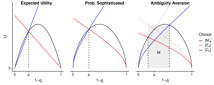
Figure 1: The value of the three choices $[E_{q}],[C_{q}]$, and $[M_{q}]$ depending on $1-q$. The left plot illustrates the utility functional under SEU, the middle plot under probabilistically sophisticated preferences, and the right plot under ambiguity-averse preferences.

First, consider an illustration of how mixing can reveal ambiguity aversion. The elementary building block of mixing bets is the choice between

• a lottery that pays with probability $q$ if the event $E$ realizes (“betting on the event”),

• a lottery that pays with probability $1-q$ if the event $E$ does not realize (“betting on the complement”), and

• a lottery that pays with probability $q(1-q)$ (“mixing”).

The lottery $[M_{q}]$ can be interpreted as a probabilistic mixture of option $[E_{q}]$ and option $[C_{q}]$ that does not dependent on the potentially ambiguous event $E$. Figure 1 illustrates the value associated with each choice for SEU preferences, probabilistically sophisticated preferences [45], and ambiguity-averse preferences. All three examples assign the ambiguity-neutral probability $p$ to the event $E$. Under all preferences, the option $[C_{q}]$ becomes more attractive and the option $[E_{q}]$ less attractive with increasing $1-q$. The value $1-q$ at which the decision-maker switches between the choice $[E_{q}]$ and $[C_{q}]$ can be used to elicit the subjective probability $p$.

Under SEU, the value of $[E_{q}]$ and $[C_{q}]$ is linear in $q$. Further, the decision-maker is indifferent between the mixture $[M_{q}]$ and its elements $[E_{q}]$ and $[C_{q}]$ if those have equal value. There exists no $q$ such that the mixing choice $[M_{q}]$ is the unique best response. The same holds for probabilistically sophisticated preferences, where values are monotonically transformed and the best response remains unaffected.

Under ambiguity aversion, the value of the mixing choice $[M_{q}]$ remains unchanged, the ambiguous choices $[E_{q}]$ and $[C_{q}]$, however, are less attractive. Thus, the mixing choice $[M_{q}]$ is the best response for some interval $M$ of values $1-q$. In particular, the set $M$ contains the probability $p$ associated with ambiguity-neutral preferences. Further, the set $M$ is larger for more ambiguity-averse preferences.

1.3 Mixing bets and the belief interval

To reveal the belief interval and ambiguity attitude, I propose the following mechanism that contains the prospects $[E_{q}],[C_{q}]$, and $[M_{q}]$ from Section 1.2 as special cases. The agent is endowed with lottery tickets, where each ticket represents a fixed probability to win a prize (e.g., a monetary reward). The agent has to bet each ticket on the event or its complement. The two events have different betting odds. If the event realizes, the agent obtains the tickets placed on the event multiplied by the odds of the event. Otherwise, she obtains the tickets placed on the complement multiplied by the odds of the complement. This task is called a mixing bet and it is repeated with different odds, where one instance is randomly selected for payout. The best response depends on the ratio between the odds of the event and the odds of the complement denoted as odds quota $q$.

The lottery tickets guarantee robustness to the unknown utility function [54] if the randomization device is perceived as independent lottery. Paying out only one mixing bet is meant to prevent hedging across the repeated betting tasks [4, 5, 10, see].

I establish the following results: Under the ambiguity-averse preferences considered above, mixing (betting tickets on the event and the complement) is a sufficient condition for the odds quota being in the belief interval. Beliefs are ambiguous (i.e., they do not reduce to a single probability level) if and only if the agent mixes for at least two different quotas. Further, the intensity of mixing reveals aspects of ambiguity attitude with maxmin (and Choquet) preferences inducing the most extreme mixing.

Further, I propose a generalization of mixing bets with two separate choices that reveals the belief interval for ambiguity-seeking and ambiguity-averse preferences.

1.4 Experimental evidence

In a laboratory experiment, the mechanism is applied to events generated by an Ellsberg urn, by a stock index, and by another participant’s behavior in a prisoner’s dilemma game. I propose three indices based on mixing bets to quantify different aspects of ambiguity-sensitive preferences. The midpoint of the mixing interval measures the ambiguity-neutral probability, the length of the mixing interval reflects ambiguity perception, and the intensity of mixing provides additional information on ambiguity attitude.

Providing evidence for the validity of mixing bets, ambiguity perception is highest for the ambiguous and lowest for the risky category in the Ellsberg urn. After observing additional draws from the urn, the measured ambiguity decreases. Interestingly, ambiguity perception for the natural events, generated by the stock index and another participant’s behavior, is almost as large as for the Ellsberg urn. This suggests that ambiguity can be important in real-world decision making.

The experimental evidence suggests that the intensity of mixing is an individual-specific property that provides additional information next to the mixing interval. Only a small share of participants behaves consistently with the extreme mixing predicted by maxmin preferences. Instead, mixing is often found to be more moderate, which is consistent with variational or second-order preferences.

I find that experience with uncertainty is negatively correlated with ambiguity perception for the stock index and the risky draw from the urn, but not with ambiguity perception for the ambiguous draw or the other participants’ behavior. Cooperation in the prisoner’s dilemma is correlated with the midpoint of the mixing interval (indicating reciprocity), but not with risk aversion, ambiguity aversion, or ambiguity perception.

1.5 Related Literature

This paper introduces a novel mechanism that reveals ambiguity, shows its validity under a wide range of preferences, and provides experimental evidence on its applicability.

The most closely related literature uses matching probabilities [19, 8] to elicit ambiguity. [6] propose belief hedges to construct indices of ambiguity attitude and perception based on the matching probabilities of three mutually exclusive events and their pairwise unions. [7] show that their indices are insightful under a wide range of ambiguity-sensitive models.

Belief hedges have been applied productively in the literature. [42] apply the method in an adapted trust game where the second player has an additional third option and [2] elicit ambiguity perception about different assets from a sample of investors by dividing the return values into three intervals. [31] experimentally investigates the ambiguity perception index after eliciting matching probabilities based on three intervals of temperature. Note that all applications relied on three events, where a single event (and its complement) would have been sufficient.

While the index of ambiguity aversion [7, Def. 6,] is applicable for a single event, the index of ambiguity-generated-insensitivity [7, Def. 10,] requires at least three events. For a single event, mixing bets provide richer information by revealing the mixing interval and the intensity of mixing simultaneously. In many applications, only a single event is of interest (e.g., becoming jobless, bank default, regime change, nuclear war) and the construction of three mutually exclusive events is an unnecessary complication.

Related elicitation work obtained identification results at the expense of generality across decision models or the simplicity of the mechanism. [12] extend the mechanism introduced by [34] to $\alpha$-maxmin preferences. In another paper, [13] introduce a mechanism that identifies the distribution of beliefs for second-order preferences.

So far, applied studies rely mostly on proxies for ambiguity. [14] use the marginal distribution of intra-day data, [3] the disagreement between professional forecasters, [51] the deviation between probabilistic forecast and realization, and [41] return volatility. Other applied work considers the relation between the object of interest and ambiguity attitude measured on artificial events like the Ellsberg urn. See for example [49] for consumer and [11] for portfolio choice. [55] find that prosocial behavior in a prisoner’s dilemma is correlated with ambiguity tolerance measured on an artificial event. I find no correlation between cooperation in the prisoner’s dilemma and ambiguity measured on the actually relevant event (the other participant’s behavior). Instead, the ambiguity-neutral probability, measured by the midpoint of the mixing interval, is the most relevant predictor suggesting reciprocity to be more important than ambiguity.

Next to revealing subjective ambiguity, mixing bets can empirically distinguish between some models of ambiguity. Differentiating between ambiguity-sensitive preferences has been considered before with artificially designed events like the Ellsberg urn [17, 18, e.g.,]. In an incentivized experiment with mixing bets I provide complementary evidence considering ambiguity generated by two natural sources of uncertainty: The stock market and the behavior of other participants. I find that most participants’ behavior is consistent with moderate ambiguity aversion as in smooth or variational preferences and in contrast to the extreme mixing implied by maxmin (and Choquet) preferences.

In the next section, the key findings of the paper are summarized. For technical details see Section 3, where the mixing behavior under different preferences is derived. Sections 3.1 to 3.3 cover maxmin, variational, and second-order preferences respectively. Section 4 introduces a generalization, separated mixing bets, which reveal ambiguity-seeking and ambiguity-averse preferences simultaneously. Section 5 provides an experimental implementation and empirical evidence. Section 6 concludes. Proofs are provided in the appendix. Other ambiguity-averse preferences, e.g. biseparable preferences [24] that include $\alpha$-maxmin [48, 23] and Choquet expected utility [53], do not allow for a similar separation of a belief interval from ambiguity attitude. A supplementary document discusses mixing bets under those preferences and under general ambiguity-averse preferences [15].

2 Mixing and the Belief Interval

Consider the task of eliciting beliefs about an event $E$ from an agent with unknown preferences. The state space is given by $S=\{E,E^{c}\}\times[0,1]$, where any state $s\in S$ describes the realization of the event $E$ and the independent random draw $r$ of the elicitation mechanism. The agent’s preferences $\succeq$ are defined on acts $l:S\mapsto\mathcal{X}$ that assign an outcome to each state. The set of all acts is denoted by $\mathcal{F}$.

In the first part of the paper, some kind of aversion to ambiguity is assumed within one of several ambiguity-sensitive preferences.

Regularity Conditions 1 (ambiguity aversion).

The agent has ambiguity-averse smooth second-order or variational preferences, where the random draw $r$ is independent of $E$ and uniformly distributed.

Essentially, Regularity Conditions 1 imply expected utility for the lottery (risk) and ambiguity aversion for acts that depend on the event $E$. Regularity Conditions 1 contain maxmin preferences as a special case. Note that the assumption on the random draw $r$ has to be formulated differently depending on the preference class at hand. Similarly, the exact definition of ambiguity aversion depends on the class of preferences. For details see Regularity Conditions 3 for maxmin, Regularity Conditions 4 for variational, and Regularity Conditions 5 for second-order preferences.

Following [38], we capture perceived ambiguity by the range of relevant probabilities.

Definition 1 (belief interval).

The belief interval $B$ is defined as the smallest closed interval that contains all relevant probability levels.

[38] provide a behavioral definition of relevant probabilities in smooth models that coincides with the belief interval for maxmin and second-order preferences. Heuristically, the belief interval $B$ denotes the relevant probabilities $p$ that the agent considers when making decisions related to the uncertain event $E$. Section 3 provides details on the uniqueness of the belief interval. For simplicity, I consider only belief intervals instead of arbitrary sets.

For SEU preferences, the belief interval $B=\{p\}$ can be denoted by a unique probability $p$ on the unit interval. Ambiguity-averse preferences, however, take into account a range of probability levels.

Definition 2 (ambiguous beliefs).

Preferences are said to exhibit ambiguous beliefs about the event $E$ if the belief interval $B$ is not a single point.

Next, we turn to the elicitation mechanism. The elementary building block can be described as follows.

1. The agent chooses the ratio $x$ of lottery tickets that she bets on the event $E$ (and the remainder $1-x$ on its complement $E^{c}$).

2. If the event $E$ realizes, the agent receives $xq$ lottery tickets. If the complement $E^{c}$ realizes, the agent receives $(1-x)(1-q)$ lottery tickets.

3. The agent is rewarded with the fixed prize $w$ if her ticket amount exceeds a random variable $r$ that is uniformly distributed on $[0,1]$.

Note that the choices $[E_{q}],[C_{q}]$, and $[M_{q}]$ introduced in Section 1.2 can be recovered with $x=1$, $x=0$, and $x=1-q$. Formally, a choice $x$ can be associated with an act in $\mathcal{F}$. Let $\mathbbm{1}(A)$ denote the indicator function for an event $A$.

Definition 3 (mixing bet).

The mixing bet with choice $x\in[0,1]$, odds quota $q\in[0,1]$, and prize $w\in\mathcal{X}$ is defined as the act

$$l(x,q,w):S\to\mathbb{R}:(E,r)\to w\cdot\mathbbm{1}\Big{(}xq\mathbbm{1}(E)+(1-x)(1-q)\mathbbm{1}(E^{c})>r\Big{)}.$$

The two potential outcomes of this mixing bet are $w$ and $0$. The prize $w$ is received, if the obtained tickets are larger than the random draw $r$, such that $xq$ denotes the probability of winning if the event $E$ realizes and $(1-x)(1-q)$ if the complement $E^{c}$ realizes. Throughout, it is assumed that the agent prefers to obtain the prize $w$.

The mixing interval $M$ describes all odds for which the agent is mixing between the event and the complement.

Definition 4 (mixing interval $M$).

Let $x^{\ast}(q):[0,1]\to[0,1]$ define an optimal choice for the odds ratio $q$ such that

$$l(x^{\ast}(q),q,w)\succeq l(x,q,w)\text{ for all $x\in[0,1]$.}$$

The mixing interval $M$ is defined as the smallest closed interval that contains

$$\{q\in[0,1]\;|\;x^{\ast}(1-q)\in(0,1)\}.$$

Trivially, the optimal choice is $x^{\ast}(q)=1$ (betting all lottery tickets on the event $E$), if the quota $q$ is large enough. The resulting act is $[E_{q}]$ from Section 1.2, a lottery with probability $q$ if the event realizes. Similarly, the optimal choice is $x^{\ast}(q)=0$ (betting all lottery tickets on the complement $E^{c}$), if the quota $q$ is small enough. The resulting act is $[C_{q}]$, a lottery with probability $1-q$ if the complement realizes. Both acts depend on the potentially ambiguous event $E$. If the agent bets $x^{\ast}(q)=1-q$ on the event, the resulting act is $[M_{q}]$, a lottery with probability $q(1-q)$ irrespective of the uncertain event $E$. The ambiguity cancels out. An ambiguity-averse agent prefers to mix between the two events to hedge against ambiguity. The higher the ambiguity aversion, the closer moves the optimal choice towards $1-q$. The main result of the paper establishes that mixing reveals ambiguity aversion and partially identifies the belief interval.

Theorem 1 (belief interval).

Under Regularity Conditions 1, mixing for a quota $q$ implies that $1-q$ is an element of the belief interval,

$$M\subset B.$$

In addition, beliefs are ambiguous if and only if there exist at least two different odds quotas $q$ for which the agent prefers to mix.

Theorem 1 is established in Section 3 for each class of preferences separately. This result allows to bound the belief interval from within and to identify ambiguous beliefs. Note that the set of odds $1-q$ for which the agent chooses $[M_{q}]$ is a subset of the mixing interval $M$. Thus, the simple choice from Section 1.2 is sufficient to bound the belief interval. However, the mixing interval $M$ provides sharper bounds for the belief interval and the intensity of mixing reveals additional information on ambiguity attitude.

The partial identification of the belief interval $B$ can be strengthened. Additional considerations allow to separate the belief interval (ambiguity perception) from the ambiguity attitude. Under maxmin preferences, it holds that

$$M=B$$

and that the mixing is extreme with $x^{\ast}(q)=1-q$.

For variational preferences, an unbounded utility difference $u_{w}\mathrel{\mathop{:}}=u(w)-u(0)$ and a bounded first derivative of the cost function $c$ guarantee the existence of a sufficiently attractive prize $w$ such that

$$M_{u_{w}}=B,$$

and more ambiguity-averse preferences, all else equal, induce mixing choices closer to $1-q$.

For second-order preferences, a uniformly positive ambiguity aversion guarantees that the mixing interval $M_{u_{w}}$ approximately recovers the belief interval $B$ for large utility difference $u_{w}$. It holds that

$$M_{u_{w}}\to B\quad\text{for }u_{w}\to\infty.$$

For small utility differences, the mixing interval might be a poor approximation of the belief interval. I show that the mixing interval remains informative as its length is dominated by

$$-\frac{\phi^{\prime\prime}}{\phi^{\prime}}\operatorname{Var}_{p\sim\mathbb{P}}(p)\quad\text{for $u_{w}\to 0$}$$

where $-\frac{\phi^{\prime\prime}}{\phi^{\prime}}$ is a proxy for ambiguity attitude and the second-order variance $\operatorname{Var}_{p\sim\mathbb{P}}(p)$ for ambiguity perception.

In the next section, I describe the best response for ambiguity-averse preferences in detail. The reader uninterested in those details can skip to Section 4 for ambiguity-seeking preferences and Section 5 for an experimental implementation.

3 Optimal Mixing under Ambiguity Aversion

First, consider the best response to the betting mechanism for an agent with SEU preferences.

Regularity Conditions 2 (SEU).

The agent has SEU preferences with a belief $p\in[0,1]$ about the event $E$. In particular, the preferences can be represented by

$$U(l)=\mathbb{E}_{E\sim p}[u(l(E))]$$

for some strictly increasing utility function $u$.

Throughout the paper, it is assumed that the agent holds accurate beliefs about the independent uniform draw that is used in the mechanism to induce risk neutrality. For notational convenience, the distribution of $r$ is not stated explicitly. The best response under SEU is

$$x^{\ast}(q)=\operatorname*{arg\,max}_{x\in[0,1]}\;\mathbb{E}_{E\sim p}[\,u(w\mathbbm{1}(s_{q}(x,E)>r))\,],$$

where $s_{q}(x,E)=xq\mathbbm{1}(E)+(1-x)(1-q)\mathbbm{1}(E^{c}).$ First, I employ a key result from binarized scoring rules [33, compare e.g.,].

Lemma 1 (binarized score).

For any score $s$ in the unit interval, the expected utility of a lottery payout based on the score $s$ is a positive affine transformation of the expected score

$$\mathbb{E}[u(w\mathbbm{1}(s>r))]=\mathbb{E}[s]u_{w}+u(0),$$

with $u_{w}\mathrel{\mathop{:}}=u(w)-u(0)$.

Lemma 1 shows that the optimal mixing behavior for SEU preferences is independent of the agent’s utility function.

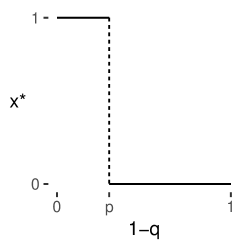
Figure 2: Optimal response for SEU preferences with belief $p=0.3$.

Lemma 2 (SEU).

The optimal choice for SEU preferences in Regularity Conditions 2 is

$$x^{\ast}(q)=\begin{cases}1&\text{if }\;p>1-q\\ [0,1]&\text{if }\;p=1-q\\ 0&\text{if }\;p<1-q.\\ \end{cases}$$

The proof of Lemma 2 is straightforward as the maximization problem can be rewritten with Lemma 1 as $x^{\ast}(q)=\operatorname*{arg\,max}\mathbb{E}_{E\sim p}[s_{q}(x,E)],$ which is linear in $x$.

The optimal choices for SEU preferences are illustrated in Figure 2. Mixing is optimal if and only if $1-q$ equals the subjective probability $p$. Otherwise, betting all lottery tickets on one event is optimal. If the elicitor observes $x(q)^{\ast}=1$, it follows that $p>1-q$. For $x(q)^{\ast}=0$, it follows that $p<1-q$. Thus, choices for different odds $q$ reveal an interval that contains the belief $p$.

3.1 Maxmin Preferences

This section establishes the optimal mixing for maxmin preferences with belief interval $B$.

Regularity Conditions 3 (maxmin).

The agent holds maxmin preferences with belief interval $B=[a,b]$ about the event $E$. In particular, the preferences can be represented by

$$U(l)=\min_{p\in B}\mathbb{E}_{E\sim p}[u(l(E))]$$

for some strictly increasing utility function $u$.

The set of measures $B$ is unique [25] and the belief interval is well-defined. As a special case, maxmin preferences contain SEU preferences if the beliefs are unambiguous with $B=\{p\}$.

Lemma 3 (maxmin).

The optimal choice for maxmin preferences as in Regularity Conditions 3 is

$$x^{\ast}(q)=\left\{\begin{aligned} &1&&\text{if }\hphantom{a<{}}1-q<a\\ &1-q\quad&&\text{if }{a}<1-q<b\\ &0&&\text{if }b<1-q\end{aligned}\right.$$

Lemma 3 follows from the more general statement for variational preferences in Lemma 4. See Lemma LABEL:th:betsalphamaxmin in the supplementary document for $\alpha$-maxmin preferences.

Interpreting betting behavior for maxmin preferences is straightforward as illustrated in Figure 3. If everything is betted on the complement $E^{c}$, the belief interval $B$ is below $1-q$. If everything is betted on $E$, the belief interval is above $1-q$. Finally, if mixing is observed, the belief interval contains $1-q$.

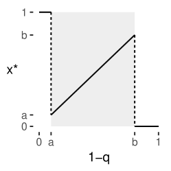
Figure 3: Optimal response for maxmin preferences with ambiguous belief interval $B=[a,b]$. The shaded area marks the belief interval, which is identified by the mixing behavior.

3.2 Variational Preferences

This section establishes the mixing behavior under variational preferences [44], which generalize multiplier preferences [29, 30]. We assume variational preferences with belief interval $B$.

Regularity Conditions 4 (variational preferences).

The agent has variational preferences. In particular, the preferences over acts $l(E)$ can be represented by

$$U(l)=\min_{p\in B}\mathbb{E}_{E\sim p}[u(l(E))]+c(p)$$

for some strictly increasing utility function $u$ and some grounded, strictly convex and twice continuously differentiable cost function $c:B\to[0,\infty)$.

The cost function $c$ is grounded such that there exists $p\in B$ with $c(p)=0$. All variational preferences are ambiguity-averse, with maxmin preferences as a special case. Regularity Conditions 4 cover variational preferences as defined in [44] if they are twice continuously differentiable and strictly convex on $\{p\in[0,1]\;|\;c(p)<\infty\}$. To see this, define a cost function $c_{c}(p)$ by

$$c_{c}(p)\mathrel{\mathop{:}}=\begin{cases}c(p)&\text{if }p\in B\\ \infty&\text{if }p\notin B\end{cases}$$

and $U(l)=\min_{p\in[0,1]}\mathbb{E}_{E\sim p}[u(l(E))]+c_{c}(p)$.

Given a utility function $u$, the minimal $c_{c}$ is unique [44, Theorem 3,] and the belief interval $B$ is defined by the closure of $\{p\in[0,1]:c_{c}(p)<\infty\}$. Rescaled utility functions represent the same preferences when paired with a rescaled cost function $c$ [44, Corollary 5,], such that the belief interval is unique.

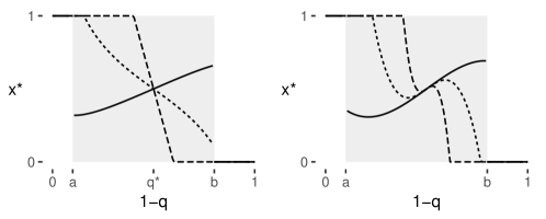
Figure 4: Optimal response for variational preferences. The optimal choice is continuous in $q$. Six examples are shown, where the belief interval is $B=[0.1,0.8]$ throughout. The left plot depicts multiplier preferences with $c(p)=\theta R(p||0.5)$ and $\theta=0.1,0.5,1.5$, where $R$ is the relative entropy function. The right plot depicts variational preferences with $c(p)=\theta|p-0.5|^{4}$ and $\theta=1,10,100$.

Lemma 4 (variational preferences).

If the agent follows variational preferences as in Regularity Conditions 4 with belief interval $B=[a,b]$, the optimal choice for a mixing bet with prize $w$ is

$$x^{\ast}(q)=\left\{\begin{aligned} &1&&\text{if }\hphantom{a<{}}1-q<a\\ &m_{w}(q)\quad&&\text{if }{a}\leq 1-q\leq b\\ &0&&\text{if }b<1-q\end{aligned}\right.$$

for a continuous function $m_{w}:B\to[0,1]$ and it holds that

1. $m_{w}(q)=1-q$ if and only if $c(1-q)=0$,

2. the mixing interval is $M_{u_{w}}=\{q\in B|c^{\prime}(1-q)/u_{w}<1-q<1+c^{\prime}(1-q)/u_{w}\}$,

3. on $M_{u_{w}}$ the mixing function is $m_{w}(q)=1-q-\tfrac{c^{\prime}(1-q)}{u_{w}}$, and

4. if $c^{\prime}$ is bounded and $u_{w}$ is unbounded, there exists a prize $w$ such that the mixing interval identifies the belief interval, $M_{u_{w}}=B.$

The rich behavior of mixing bets under variational preferences can be summarized as follows. Mixing is never optimal outside of the belief interval. Extreme mixing with $x^{\ast}(q)=1-q$ is optimal for $c(1-q)=0$, which allows to reveal the interval $\{p\in B|c(p)=0\}$. The remainder of the mixing interval exhibits less severe mixing with $x^{\ast}(q)\neq 1-q$. If the utility difference $u_{w}$ is sufficiently large, the mixing interval recovers the belief interval.

Note that the intensity of mixing reveals aspects of the ambiguity attitude as captured in the function $c$. Given a fixed utility function $u$, variational preferences become more ambiguity averse with smaller cost functions $c$ [44, compare Proposition 8,]. Consider two agents with identical belief intervals and utility functions, where $c_{2}=\lambda c_{1}$ for some $\lambda>1$ such that $c_{2}$ expresses less ambiguity aversion. The more ambiguity-averse agent mixes more intensely, i.e. $x^{\ast}(q)$ is closer to $1-q$, which allows us to order agents by ambiguity attitude.

3.3 Smooth Second-Order Preferences

This section considers smooth second-order preferences [36].

Regularity Conditions 5.

The agent holds beliefs $\mathbb{P}$ in form of a distribution over $[0,1]$ with support $B=[a,b]$ with $0\leq a\leq b\leq 1$ about the event $E$ and has ambiguity-averse smooth second-order preferences. In particular, the preferences over acts $l(E)$ can be represented by

$$U(l)=\mathbb{E}_{p\sim\mathbb{P}}[\phi(\mathbb{E}_{E\sim p}[u(l(E))])]$$

for some strictly increasing utility function $u$ and some strictly increasing, concave, and twice continuously differentiable second-order utility function $\phi$.

The second-order probabilities $\mathbb{P}$ are almost surely unique and the belief interval is unique across representations. See [38] for a theoretical discussion on capturing the perception of ambiguity under second-order preferences and beyond.

Lemma 5.

The optimal choice for a mixing bet with prize $w$ of an ambiguity-averse agent with second-order preferences as in Regularity Conditions 5 is

$$x^{\ast}(q)=\left\{\begin{aligned} &1&&\text{if }\hphantom{a<{}}1-q<a\\ &m_{w}(q)\quad&&\text{if }{a}\leq 1-q\leq b\\ &0&&\text{if }b<1-q,\end{aligned}\right.$$

for some continuous function $m_{w}:B\to[0,1]$ such that for all $w$

• $m_{w}(1-a)=1$ and $m_{w}(1-b)=0$

• $m_{w}(1-q)<1$ if $1-q>\mathbb{E}_{p\sim\mathbb{P}}[p]$ and $m_{w}(1-q)>0$ if $1-q<\mathbb{E}_{p\sim\mathbb{P}}[p]$.

In particular, it holds that $\mathbb{E}_{p\sim\mathbb{P}}[p]\in M_{u_{w}}$. Further, if the coefficient of ambiguity aversion $\alpha(z)=-\tfrac{\phi^{\prime\prime}(z)}{\phi^{\prime}(z)}$ is bounded away from zero, it holds that

$$M_{u_{w}}\to B\quad\text{for }u_{w}\to\infty.$$

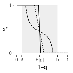
Figure 5: Optimal response for second-order ambiguity-averse preferences. The optimal choice is continuous in $q$ and lies in the shaded rectangle. Three examples are shown, where $u(0)=0$, $u(w)=1$, the second-order distribution $\mathbb{P}=U[0.1,0.8]$ and the second-order utility function is $\phi(z)=-e^{-\theta z}$ with $\theta=1,4,16$ respectively.

The continuity of $m_{w}$ implies that the agent is mixing on an interval of positive length. For sufficiently strong ambiguity aversion second-order preferences are essentially identical to maxmin preferences [36] and the belief interval can be identified with a high degree of accuracy. Lemma 5 shows that the same effect can be induced by increasing the utility difference $u_{w}$ if one is willing to assume strictly positive ambiguity aversion.

In Figure 5 three examples with different constant absolute ambiguity aversion are shown. Bounds on the belief interval are conservative for moderate rates of ambiguity aversion and low utility difference $u_{w}$ between prizes.

The exact determination of the belief interval with moderate utility differences $u_{w}$ is complicated by the interaction between perception (represented by $\mathbb{P}$) and attitude (represented by $\phi$ and $u$). For small utility differences $u_{w}$, the following lemma establishes that the mixing behavior is informative about $\operatorname{Var}_{p\sim\mathbb{P}}(p)$, which constitutes another proxy for ambiguity perception for smooth second-order preferences.

Lemma 6.

Given smooth second-order preferences as in Regularity Conditions 5 with thrice continuously differentiable second-order utility $\phi$, the length of the mixing interval can be approximated by

$$-\frac{\phi^{\prime\prime}(u(0))}{\phi^{\prime}(u(0))}\operatorname{Var}_{p\sim\mathbb{P}}(p)u_{w}$$

for small utility differences $(u_{w}\to 0)$.

In particular, it follows that mixing bets allow comparing ambiguity perception (under identical ambiguity attitude). While the mixing interval vanishes for $u_{w}\to 0$, it has a positive length for any $u_{w}>0$ and the rate of decline is approximately proportional to the product of local ambiguity aversion at $u(0)$ and the variance of the second-order distribution $\mathbb{P}$.

Large utility differences $u_{w}$ inform about the support of $\mathbb{P}$ (Lemma 5) and low utility differences $u_{w}$ inform about the variance of $\mathbb{P}$ (Lemma 6). Note that if $\mathbb{P}$ comes from a location-scale family, either measure can be used to infer the scale of $\mathbb{P}$.

The above lemma makes the smooth second-order preferences operational. While the interaction of higher moments of $\mathbb{P}$ and higher derivatives of $\phi$ remain elusive, the main characteristics, namely the ambiguity-neutral probability $\mathbb{E}_{p\sim\mathbb{P}}[p]$ and some proxy for ambiguity perception, are available for large and small utility differences. Importantly, a typical assumption would be that attitude in form of $\phi$ and $u$ remains constant for an individual irrespective of learning or the target event $E$. Thus, the difference in mixing elicited from the same person for two events is informative about the difference in ambiguity perception.

Lemma 6 is closely related to an observation in [7], who consider a specific series of events with vanishing ambiguity and find that their ambiguity aversion index is also dominated by $\tfrac{\phi^{\prime\prime}}{\phi^{\prime}}\operatorname{Var}(p).$ Conveniently, Lemma 6 above applies to all events and the utility difference $u_{w}$ can be controlled by the researcher, whereas the limit construction in [7] is more of theoretical nature.

4 Ambiguity-seeking Preferences

The mixing bets considered until here cannot identify ambiguous beliefs for ambiguity-seeking preferences. While ambiguity aversion is more prominent empirically, it is by no means universal [43]. This section introduces a generalization, separated mixing bets, that allows to distinguish between ambiguity-seeking and ambiguity-averse preferences and to identify the belief interval irrespective of ambiguity attitude.

4.1 Illustration: Separated Mixing Bets

To build intuition, consider an extension of the illustration from Section 1.2 to ambiguity-seeking preferences as depicted in Figure 6. Again, we analyze the value of the three choices $[E_{q}]$, $[C_{q}]$, and $[M_{q}]$ (betting on the event, the complement, and mixing) under different preferences.

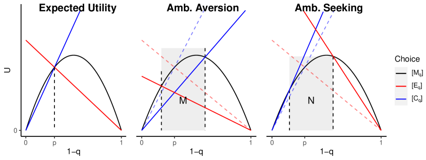
Figure 6: The value of the three choices $[E_{q}],[C_{q}]$, and $[M_{q}]$ depending on $1-q$. The left plot illustrates the utility functional under SEU, the middle plot under ambiguity-averse, and the right plot under ambiguity-seeking preferences.

First, we observe that mixing is never the best response under ambiguity-seeking preferences. The choice $[M_{q}]$ is dominated by $[E_{q}]$ (for low $1-q$), $[C_{q}]$ (for high $1-q$), or both (for intermediate $1-q$). The behavior for standard mixing bets would be indistinguishable from SEU.

Instead, the difference between SEU and ambiguity-seeking preferences arises if the choice between $[M_{q}]$ and its components is observed separately. An ambiguity-seeking agent prefers the ambiguous bets $[E_{q}]$ and $[C_{q}]$ over the unambiguous $[M_{q}]$ for some values of $1-q$. We refer to this interval as the non-mixing interval $N$.

4.2 Separated Mixing Bets

Consider the following ambiguity-seeking preferences.

Regularity Conditions 6 (ambiguity seeking).

The agent has ambiguity-seeking smooth second-order or maxmax preferences, where the random draw $r$ is independent of $E$ and uniformly distributed.

Separated mixing bets are a generalization of the mixing bets considered before. The agent chooses twice, where in each choice the options are limited to allocations of lottery tickets that favor one of the two outcomes. For the odds quota $q$, the feasible allocations are restricted to $[1-q,1]$ (favoring the event) and $[0,1-q]$ (favoring the complement).

In this scenario, the mixing interval $M$ describes all odds for which the agent is mixing in both separated mixing bets. Additionally, the non-mixing interval $N$ describes all odds for which the agent is not mixing in either of the two separated mixing bets. Note that the mixing interval recovers the information from the simple mixing bets considered before. The non-mixing interval provides additional information for ambiguity-seeking preferences.

Definition 5 (mixing interval $M$ and non-mixing interval $N$).

Let $x_{E}^{\ast}(q):[0,1]\to[1-q,1]$ and $x_{C}^{\ast}(q):[0,1]\to[0,1-q]$ define the optimal choice for the odds ratio $q$ such that

$$l(x_{E}^{\ast}(q),q,w)\succeq l(x,q,w)\text{for all $x\in[1-q,1]$,}$$

$$l(x_{C}^{\ast}(q),q,w)\succeq l(x,q,w)\text{for all $x\in[0,1-q]$}.$$

The mixing interval $M$ is defined as the smallest closed interval that contains

$$\{q\in[0,1]\;|\;x_{E}^{\ast}(1-q)\in(0,1)\text{ and }x_{C}^{\ast}(1-q)\in(0,1)\}.$$

The non-mixing interval $N$ is defined as the smallest closed interval that contains

$$\{q\in[0,1]\;|\;x_{E}^{\ast}(1-q)\notin(0,1)\text{ and }x_{C}^{\ast}(1-q)\notin(0,1)\}.$$

Trivially, the optimal choices are $x_{E}^{\ast}(q)=1$ and $x_{C}^{\ast}(q)=1-q$ (betting as many lottery tickets on $E$ as possible), if the quota $q$ is large enough. Similarly, the optimal choice is $x_{E}^{\ast}(q)=1-q$ and $x_{C}^{\ast}(q)=0$ (betting as many lottery tickets on $E^{c}$ as possible), if the quota $q$ is small enough. An ambiguity-averse agent prefers to mix for the two separated bets and the mixing interval is non-empty. An ambiguity-seeking agent prefers the two ambiguous extremes to the mixing and the non-mixing interval $N$ is non-empty. The main result of this section is that non-mixing (the choice $x^{\ast}_{E}(q)=1$ and $x^{\ast}_{C}(q)=0$) implies ambiguous beliefs and ambiguity-seeking preferences.

Theorem 2 (belief interval and non-mixing).

Under Regularity Conditions 6, non-mixing for a quota $q$ implies that $1-q$ is an element of the belief interval,

$$N\subset B.$$

In addition, beliefs are ambiguous if and only if there exist at least two different odds quotas $q$ for which the agent prefers not to mix in both separated mixing bets.

Theorem 2 is established below for each class of preferences separately. The result allows to bound the belief interval from within. While small non-mixing intervals can only be detected if appropriate odds are applied, the theorem states that such odds always exist. The identification result for the belief interval $B$ can be strengthened further for maxmax preferences, where the non-mixing interval reveals the belief interval, i.e. $N=B.$

4.3 Maxmax Preferences

This section establishes the optimal mixing in separated mixing bets for maxmax preferences with belief interval $B$. Maxmax preferences arise as the most ambiguity seeking special case of $\alpha$-maxmin expected utility preferences [48, 23].

Regularity Conditions 7 (maxmax).

The agent holds maxmax preferences with belief interval $B=[a,b]$ about the event $E$. In particular, the preferences can be represented by

$$U(l)=\max_{p\in B}\mathbb{E}_{E\sim p}[u(l(E))]$$

for some strictly increasing utility function $u$.

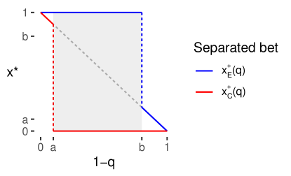
Figure 7: Optimal response for maxmax preferences with ambiguous belief interval $B=[a,b]$. The shaded area marks the belief interval, which is identified by the mixing behavior.

Lemma 7 (maxmax).

The optimal responses for the separated mixing bets for maxmax preferences as in Regularity Conditions 7 are

$$x_{E}^{\ast}(q)=\left\{\begin{aligned} &1&&\text{if }1-q<b\\ &1-q\quad&&\text{if }1-q>b\\ \end{aligned}\right.\quad\text{ and }\quad x_{C}^{\ast}(q)=\left\{\begin{aligned} &0&&\text{if }a<1-q\\ &1-q\quad&&\text{if }a>1-q\\ \end{aligned}\right.$$

The results of Lemma 7 are illustrated in Figure 7. The proof follows from the arguments in the general statement in Lemma LABEL:th:betsalphamaxmin in the supplementary document for $\alpha$-maxmax preferences.

Interpreting betting behavior for maxmax preferences is straightforward. If the decision-maker is not choosing to mix for either of the two mixing bets, then $1-q$ is in the belief interval and the preferences are ambiguity seeking. If the decision-maker chooses to mix in both separated mixing bets, then $1-q$ is in the belief interval and the preferences are ambiguity averse. If the decision-maker chooses the pure event in one and mixes for the other bet, then $1-q$ is beyond the belief interval and no statements about the ambiguity attitude can be made.

4.4 Smooth Second-Order Preferences

This section extends the results for second-order preferences from Section 3.3.

Regularity Conditions 8.

The agent holds beliefs $\mathbb{P}$ in form of a distribution over $[0,1]$ with support $B=[a,b]$ with $0\leq a\leq b\leq 1$ about the event $E$ and has ambiguity-seeking smooth second-order preferences. In particular, the preferences over acts $l(E)$ can be represented by

$$U(l)=\mathbb{E}_{p\sim\mathbb{P}}[\phi(\mathbb{E}_{E\sim p}[u(l(E))])]$$

for some strictly increasing utility function $u$ and some strictly increasing, convex, and twice continuously differentiable second-order utility function $\phi$.

Regularity Conditions 8 are identical to the assumption in Section 3.3 except for the convex second-order utility function $\phi$.

Lemma 8.

The optimal mixing for a mixing bet with prize $w$ of an ambiguity-averse agent with second-order preferences as in Regularity Conditions 8 is

$$x_{E}^{\ast}(q)=\begin{cases}1&\text{if }\mathbb{E}_{p\sim\mathbb{P}}[p]+\epsilon>1-q\\ 1-q&\text{if }b\leq 1-q\\ \end{cases}\qquad\text{and}\qquad x_{C}^{\ast}(q)=\begin{cases}0&\text{if }\mathbb{E}_{p\sim\mathbb{P}}[p]-\epsilon<1-q\\ 1-q&\text{if }a\geq 1-q\\ \end{cases}$$

for some $\epsilon>0$. In particular it holds that $\mathbb{E}_{p\sim\mathbb{P}}[p]\in N_{u_{w}}$.

Note that the non-mixing is guaranteed in an environment around $\mathbb{E}_{p\sim\mathbb{P}}[p]$. Without additional assumptions, the best response may shift multiple times beyond said environment and the end of the belief interval, where mixing is the dominant strategy for $x_{E}^{\ast}(q)$ or $x_{C}^{\ast}(q)$.

5 Implementation

I provide empirical evidence that mixing bets are feasible, measure ambiguity, and can generate insightful evidence. The focus is on mixing bets, omitting separated mixing bets from Section 4.

5.1 Experimental Setup

In a pilot laboratory experiment, 88 student subjects were recruited at the Frankfurt Laboratory for Experimental Economic Research (FLEX). The experiment was implemented with OTree. The average age was 25 and $49\%$ of participants were female. Most participants studied economics or business (38%), mathematics or natural sciences (14%), social science (14%), or law (14%).

Participants received 5 Euros for participation. First, they played a standard prisoner’s dilemma with potential payoffs of 1 Euro (both defect), 2 Euros (both cooperate) and 0/3 Euros (cooperate/defect). Next, risk aversion was measured with a choice between 2 Euros, 5 Euros with a $50\%$ chance, and 10 Euros with a $30\%$ chance. The probabilities were generated by drawing a number from 1 to 100 from a box. The same mechanism was used subsequently as the randomization device in the mixing bets. Participants could win a prize of 10 Euros with the mixing bets. Before the mixing bets elicitation, participants received instructions, examples, and test questions for the payoff mechanism. At the end of the experiment, demographic data were collected, the realization of the events was shown and an envelope was opened that contained the mixing bet number that would determine the payout. Then, the number of obtained lottery tickets was shown on the screen and each participant had to draw a number from a box to determine the final payoff.

In the main part of the experiment, I revisit the Ellsberg urn with an urn that contains 90 balls, where the color composition (60 red, 30 blue) was known, but the number of dotted balls (0 - 60 dotted) was unknown. Further, the current value of the German Stock Index was written down at the beginning of the experiment (before the German Stock Exchange opened) and at the end of the experiment (about 30 minutes after trading started).

In total, five different domains were considered: The event of a blue ball being drawn (risk), the event of a dotted ball being drawn (ambiguity), the event of the stock market rising (stock), the event of the assigned player in the prisoner’s dilemma choosing to defect (social). The order of elicitation was randomized for each participant. Finally, all participants were shown 10 draws from the Ellsberg urn and repeated the dotted ball elicitation (updated). For each domain the quotas $q\in\{0.1,0.2,\dots,0.9\}$ were applied, where the order was randomized and the values above (below) were skipped if a higher (lower) quota elicited the answer $x=0$ ($x=1$). If the procedure finished with four or fewer quotas considered, an additional choice for another quota $q$ was elicited to check the consistency. Throughout odds were scaled such that betting all tickets on one event implied certainty.

I consider two ways of framing the elicitation with mixing bets. In the discrete elicitation, participants encounter a series of pairwise choices representing the three extreme choices $x\in\{0,1-q,1\}$ from Section 1.2. A single decision in the discrete elicitation is relatively simple as illustrated by the following example.

What do you prefer? 10 Euros if $\dots$

• $\dots$ a red ball will be drawn and additionally you draw a number between 1 and 25.

• $\dots$ a blue ball will be drawn.

In the continuous elicitation participants could choose $x$ with a slider, where for each slider position the payoff for the two events was shown on the screen (e.g., for the middle position $x=0.5$ with quota $q=0.5$ the screen shows “If the stock index rises, you will receive 10 Euros if you draw a number between 1 and 50.” and “If the stock index declines, you will receive 10 Euros if you draw a number between 1 and 50.”.). Feasible allocations were reduced to $x\in\{0,0.1,\dots,0.9,1\}$. The continuous elicitation followed after the discrete elicitation and to avoid excessive waiting times, it was skipped if a participant fell behind too much for the updated, stock, and social domain, but not for the risk and ambiguity domain. About 50% of participants were subject to the continuous elicitation for all domains.

5.2 Experimental Evidence

First, we evaluate if mixing bets were conceptually understood by the participants. After the elicitation and before seeing the results, 78% of participants affirmed that they “completely understood the payout mechanism”. This subjective assessment was not correlated with gender, area of study, or experience in statistics. Another indicator is the consistency of answers. In total, $8\%$ of answers exhibit non-mixing between mixing quotas. Another $2\%$ bet on the event while betting on the complement for lower quotas. The remaining $90\%$ of answers are consistent with the choice patterns derived in Section 3.

Multiple mixing implies ambiguity aversion (Theorem 1). 82% of participants show such behavior in at least one of the three domains ambiguity, social, and stock. Within-subject heterogeneity is prominent with only 32% of participants exhibiting multiple mixing for all three domains.

Ambiguity-seeking preferences imply non-mixing for all quotas. Only $3\%$ of participants never preferred mixing, providing strong evidence against universal ambiguity seeking. However, 48% of the participants did not mix for at least one of the three domains such that a moderate prevalence of source-specific ambiguity seeking cannot be ruled out. As separated mixing bets were not elicited, the experimental setting cannot distinguish between ambiguity-seeking and ambiguity-neutral preferences.

To quantify different aspects of mixing bets, I propose three indices: the midpoint of the mixing interval, the length of the mixing interval, and the intensity of mixing. The indices can be derived directly from mixing choices and can be interpreted as ambiguity-neutral probability, ambiguity perception, and ambiguity aversion.

The first index is the midpoint of the mixing interval, or if no mixing occurred, the midpoint of the switching interval. It can be interpreted as the ambiguity-neutral probability. For maxmin and variational preferences, it approximates the midpoint of the belief interval and for second-order preferences the mean of the second-order distribution.

The second index is the length of the mixing interval, i.e. the difference between the highest and lowest quota that induced a mixing response. For maxmin preferences, it denotes the size of the belief interval (Lemma 3). For variational preferences, it does so if the prize is sufficiently attractive (Lemma 4). For second-order preferences, the separation of attitude and perception is more challenging and the length of the mixing interval identifies the size of the belief interval only for high stakes (Lemma 5) and is dominated by an interaction of the belief interval and the second-order utility for low stakes (Lemma 6).

As we can only observe choices for a finite number of quotas $q$, the measured length of the mixing interval is weakly smaller than its true length. The sharpness of the bounds can be controlled with the choice of quotas $q$. With the quotas $q\in\{0.1,0.2,\dots,0.9\}$, it follows that the difference is smaller than $0.2$.

The third index is the intensity of mixing, where extreme mixing is $x_{q}=1-q$ and the least mixing is $x_{q}=0.1$ or $x_{q}=0.9$. The intensity index is given by the average of

$$i(x_{q},q)\mathrel{\mathop{:}}=\begin{cases}x_{q}/(1-q)&\text{if }x_{q}\leq 1-q,\\ (1-x_{q})/q&\text{if }x_{q}>1-q.\\ \end{cases}$$ (1)

for all $q$ where participants chose to mix, i.e. $x_{q}\notin\{0,1\}$. The intensity of mixing is measured with the continuous elicitation as the discrete elicitation allowed only extreme mixing. For maxmin preferences, the intensity is $1$ (Lemma 3). For variational preferences, the intensity of mixing allows ranking cost functions by ambiguity aversion (Lemma 4). Note, however, that outcome-dependent preferences require the utility difference to be adequate. Low utility differences induce no mixing and high utility differences induce strong mixing.

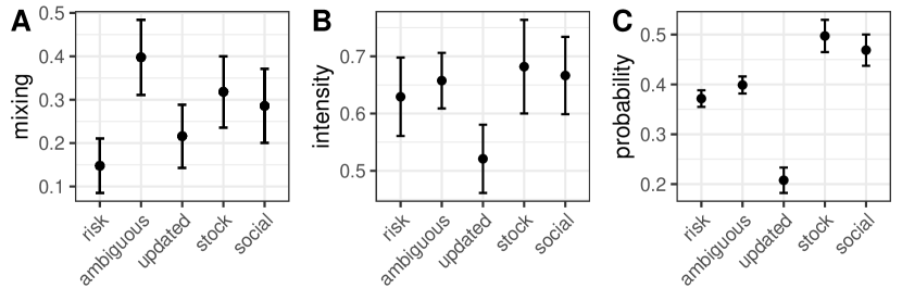
Figure 8: Proxies for ambiguity and probability perception. The plot depicts the average and its $90\%$-confidence intervals for the proxies. Panel A considers the occurrence of a mixing interval with positive length, panel B the mixing intensity as given in Equation (1), and panel C the ambiguity-neutral probability. Panel A and C depend on the discrete and panel B on the continuous elicitation.

Figure 8 shows the average of the three proxies by domain. Panel A considers the likelihood of a mixing interval with positive length. Mixing is least prevalent for the risky urn and most prevalent for the ambiguous urn (but decreasing sharply after 10 draws were shown). The two natural events, stock and social, exhibit a likelihood of mixing that is lower than the ambiguous draw ($p$-value of $t$-tests: $0.27$ and $0.13$), but higher than the risky draw ($p$-value of $t$-tests: $0.01$ and $0.03$).

The main goal of the experiment is to reveal ambiguity beyond the Ellsberg urn. The two examples considered here indicate that natural events, where uncertainty is generated by mechanisms beyond the experimental control, are indeed perceived as ambiguous by a considerable ratio of participants. Note that the German stock index should be familiar to the participant pool, which suggests even higher ambiguity perception for less commonly known stocks [1].

In panel B, the intensity of mixing is similar across sources, consistent with the idea that mixing intensity reveals a personal ambiguity attitude instead of ambiguity perception. The exception is the updated domain, where the beliefs are closer to zero and the limited allocations of $x\in\{0,0.1,\dots,0.9,1\}$ could distort measurements.

In panel C, the ambiguity-neutral probabilities are consistent with reality. The average for the risky urn is close to the true value $\tfrac{1}{3}$ and for the ambiguous urn only slightly higher. After the 10 additional draws, the average belief for the ambiguous category is updated in the direction of the true value $\tfrac{1}{10}$. The stock market is expected to rise with an average probability of $50\%$. In the cooperation game, participants expect their partner to defect with an average probability of $45\%$. The observed average was close with $46\%$ of participants defecting.

	Dependent variable:
	mixing	risk	multiple mixing
	intensity	aversion	risk	ambiguous	stock	social
	(1)	(2)	(3)	(4)	(5)	(6)
risk aversion $(s)$	0.002		$-$0.01	$-$0.02	$-$0.03	$-$0.01
	(0.02)		(0.04)	(0.06)	(0.05)	(0.06)
mixing intensity $(s)$		0.01	0.03	0.06	0.05	$-$0.02
		(0.07)	(0.04)	(0.05)	(0.05)	(0.05)
female	0.06	0.50∗∗∗	$-$0.002	$-$0.07	0.05	$-$0.08
	(0.05)	(0.14)	(0.09)	(0.13)	(0.12)	(0.12)
experience $(s)$	0.04	$-$0.04	$-$0.10∗∗	$-$0.04	$-$0.14∗∗	$-$0.01
	(0.02)	(0.07)	(0.04)	(0.06)	(0.05)	(0.06)
Constant	0.63∗∗∗	0.48∗∗∗	0.15∗∗	0.43∗∗∗	0.29∗∗∗	0.32∗∗∗
	(0.03)	(0.10)	(0.06)	(0.08)	(0.07)	(0.08)
Observations	88	88	88	88	88	77
R2	0.03	0.17	0.07	0.02	0.10	0.01
Note:	∗p$<$0.1; ∗∗p$<$0.05; ∗∗∗p$<$0.01

Table 1: Least squares regressions on proxies of attitude and perceptions. Covariates with marked with (s) were standardized. The standard errors are denoted in parentheses. Mixing intensity follows the definition in Equation (1) and is averaged across all domains. The social domain was not recorded for one session due to a technical failure, which results in a lower sample size of 77. Experience denotes a score constructed from the following survey questions: (i) How much experience do you have with probability theory and statistics? (Response scale: 1-7.) (ii) How much experience do you have with gambling? (Response scale: 1-7.) (iii) Did you attend a university lecture on statistics or probability theory? (iv) On average how many even numbers do you expect if throwing a six-sided dice a thousand times?

The summaries for each domain above lend some validation to the experimental procedure. Next, let us consider the more challenging task of analyzing individual-specific measurements. Only 4 participants and 8% of domain-specific choices exhibit a mixing intensity of 1. Thus, most mixing choices are more in line with variational and second-order preferences, contradicting maxmin preferences, as well as $\alpha$-maxmin (Supplementary Section LABEL:sec:app_alphamaxmin) or any other biseparable preferences (Supplementary Section LABEL:sec:app_bisep).

A participant-specific attitude for mixing intensity is supported by the variation in the mixing intensity. A regression with participant fixed effects explains 72% of this variation (adjusted $R^{2}=0.46$), whereas domain fixed effects explain only 1% (adjusted $R^{2}$ $<0$). The same regressions with multiple mixing and the midpoint of the mixing interval as dependent variables, show lower $R^{2}$ values for the participant fixed effects regressions and domain fixed effects that are different from zero. The pattern is consistent with the interpretation of those indices as ambiguity and probability perception. See Supplementary Section LABEL:sec:sup_co for the full regression results.

Table 1 shows regression results with the average mixing intensity in column (1) and risk aversion in column (2) as the dependent variable. No correlation between the two can be detected, suggesting that risk aversion and ambiguity aversion are empirically distinct features. Whereas female participants showed more risk aversion, no difference in the mixing intensity (measuring ambiguity aversion) is detectable. Columns (3) to (6) have as the dependent variable the occurrence of multiple mixing (equivalent to a mixing interval with positive length) and are based on the discrete elicitation. Neither risk aversion nor mixing intensity is consistently correlated with multiple mixing. This suggests that mixing intensity and the set of mixing quotas measure distinct aspects of ambiguity-sensitive behavior.

An additional control in Table 1 is experience which measures exposure to probability, statistics, and gambling. Experience is correlated with a reduced likelihood of multiple mixing for the risk and stock domain. One standard deviation of the score reduces the likelihood of multiple mixing from $15\%$ to $5\%$ in the risk domain and from $29\%$ to $15\%$ for the stock index. One possible interpretation is that even sources of uncertainty with clearly defined probabilities can be perceived as ambiguous if participants lack the knowledge and experience. For the ambiguous draw and the social domain, the experience index shows no strong effect, which suggests that ambiguity aversion in those domains is more profound than just a lack of experience with uncertainty.

Finally, let us consider prosocial behavior in the prisoner’s dilemma. Individual cooperation is predicted by the midpoint of the belief interval (representing the ambiguity-neutral probability) with a $p$-value $<0.001$ and an estimated effect size of $1\%$ probability of expecting cooperation increasing the likelihood of cooperation by $1.5\%$. This suggests reciprocity as the main driver of cooperation. For the remaining covariates (risk aversion, mixing intensity, length of the mixing interval) there is no evidence of an effect. The full regression results can be found in the supplementary document. Interestingly, this evidence contradicts previous studies on cooperation and ambiguity that relied on measuring ambiguity with artificial events unrelated to the social game and found a positive correlation between ambiguity tolerance and cooperation [55]. This simple example illustrates that the elicitation of subjective ambiguity for natural events can sharpen economic analysis and provide new insights.

6 Discussion

The separation of attitude and perception is a potentially insightful endeavor [46]. While the ability of ambiguity-sensitive models to achieve said separation is a matter of ongoing debate [21, 37], mixing bets can be used to elicit several different aspects of subjective ambiguity. In particular, I propose three indices that can be understood as measuring the ambiguity-neutral probability, ambiguity perception, and ambiguity attitude. This interpretation is most adequate for variational preferences that contain maxmin preferences as limiting case. For second-order preferences, the separation is more challenging as the length of the mixing interval for small stakes is dominated by an interaction term between the second-order utility function and the belief distribution. In an experimental study, I find that the three indices and risk aversion are uncorrelated, which supports their interpretation as different aspects of subjective uncertainty. I show that mixing bets can help explain economic decisions. In particular, I find that the midpoint of the mixing interval (measuring probability), but not the extent or intensity of mixing correlates with cooperation in a social game. Further, I show that mixing bets can be used to analyze the change of ambiguity perception under new information. In particular, I find that additional draws from the Ellsberg urn reduce the extent of mixing.

The main alternative to mixing bets are belief hedges [6, 7]. Belief hedges require at least three events to generate the insensitivity index that is often argued to capture ambiguity perception. Similar to mixing bets, they do not achieve a full separation for second-order preferences [7, see Observation 18]. However, belief hedges can separate ambiguity attitude and perception for the neo-additive model of [16] [9, see also].

Belief hedges are based on matching probabilities [32, e.g.,] also called choice-based probabilities [1]. Conveniently, matching probabilities can be analyzed without a mixing concept or a product state space. From a behavioral perspective, however, the direct comparison with a randomization device could be argued to be more distorting than mixing with such a device. If, for example, a participant exhibits aversion to the randomization device, matching probabilities will be higher and belief hedges understate ambiguity aversion. For mixing bets, the outcome depends on the randomization device irrespective of the participant’s choice, such that the same concerns do not arise. Comfortably, the experimental evidence for the Ellsberg urn provided here is broadly in line with a long line of experiments based on matching probabilities: On average participants avoided ambiguous uncertainty more than pure risk.

Mixing bets can be extended to multiple events. Real-valued uncertainty can be elicited after defining suitable intervals. Future research might be able to connect ideas from belief hedges and mixing bets. In applications, it can be beneficial to elicit both to adjust for measurement error by multiple measurements [26].

I show that mixing bets can be implemented in laboratory experiments and that they offer relevant and applicable information on preferences and private information. In particular, the experiment showed that not all participants perceived the risky urn as purely risk and the ambiguous urn did not induce as much ambiguity as the verbal explanation would suggest. Importantly, natural events were perceived as ambiguous, which underlines the relevance of ambiguity in economic decision-making. Finally, ambiguity and probability perception were heterogeneous, which could explain the strong variation between individuals in an international comparison of ambiguity attitudes [40].

A major concern is how the agent reacts when faced with multiple bets on the same uncertain outcome. The elicitation of ambiguity requires the agent to apply ambiguity aversion on each bet separately instead of integrating choices across bets. [10] find that about half of their ambiguity-averse participants integrate across choices, which leads to an underestimation of ambiguity aversion. This concern, however, arises generally [5] and also applies to matching probabilities.

Mixing bets have a direct connection to proper scoring rules [28] and can be seen as an application of multiple quantile elicitation as introduced in [22] to binary events. A single mixing bet is equivalent to a binarized asymmetric piecewise linear score for the point forecast of the random variable $\mathbbm{1}(E)$. Mixing bets can also be connected to early work on subjective probabilities. Preceding ambiguity-sensitive decision models, [54] proposed to define subjective probabilities by the odds that an agent agrees to bet on an event. By allowing the agent to mix, I provide a generalization of Smith’s hypothetical design and establish that mixing identifies ambiguity.

Instead of using mixing bets, one can ask participants directly for ranges of probabilities [47, 27, e.g.,]. However, ambiguity-averse decision models describe behavior, rather than thought processes. The belief interval may well have considerable explanatory power regarding an agent’s behavior, while the agent is unable or unwilling to articulate such an interval. In this case, a revealed preferences approach is more suitable.

Acknowledgments

I would like to thank Aurelien Baillon, Arup Daripa, Markus Eyting, Luca Henkel, Toru Kitagawa, Michael Kosfeld, Charles Manski, Matthias Schündeln, and Peter Wakker for insightful discussions. My work has been partially funded by the Klaus Tschira Foundation.

Appendix: Proofs

Proof of Lemma 1.

The expected utility can be expressed as a linear function of the probability of winning,

$$\mathbb{E}_{E\sim p}[u(\mathbbm{1}(s>r)w)]=\mathbb{P}[s>r]u(w)+(1-\mathbb{P}[s>r])u(0)=\mathbb{P}[s>r](u(w)-u(0))+u(0).$$

Further, from the independent uniform distribution of $r$ and as $s\in[0,1]$ it follows that

$$\mathbb{P}[s>r]=\mathbb{E}_{E\sim p}[\mathbb{E}_{r\sim U}[\mathbbm{1}(s>r)]]=\mathbb{E}_{E\sim p}[s].$$

∎

Proof of Lemma 4.

We apply Lemma 1 and obtain the simplified optimization problem

$$x^{\ast}(1-q)=\operatorname*{arg\,max}_{x\in[0,1]}\;\;\min_{p\in B}\;s_{q}(x,p)+c(p)/u_{w}.$$

The decision-maker acts as if more ambiguity averse for higher utility difference between prizes $u_{w}$ [44, Proposition 8,]. Define $c_{t}(p)=c(p)/u_{w}$ for notational convenience. $c_{t}$ is also grounded, strictly convex and twice continuously differentiable. As $c_{t}$ is convex it follows that $c_{t}^{\prime}$ is increasing and as $c_{t}$ is grounded, it follows that $c^{\prime}_{t}(a)\leq 0$ and $c^{\prime}_{t}(b)\geq 0$.

Next, we investigate $x^{\ast}(q)$ for fixed $q\in[0,1]$. Examine the minimum of

$$g_{x}(p)\mathrel{\mathop{:}}=s_{q}(x,p)+c_{t}(p)=1-x-q+xq+p(x-(1-q))+c_{t}(p).$$ (2)

The function $g_{x}$ is convex. The minimum at $p^{\ast}(x)\mathrel{\mathop{:}}=\operatorname*{arg\,min}_{p\in B}g_{x}(p)$ is characterized by $g^{\prime}_{x}(p)=x-(1-q)+c^{\prime}_{t}(p)$.

• First case: $p^{*}(x)=a$.
  In this case, $g^{\prime}_{x}(p^{*}(x))\geq 0$ or equivalently $x\geq 1-q-c^{\prime}_{t}(a)$. Further, the agent values the resulting bets as a function of $x$ by

  $$U(x) =g_{x}(a)=1-a-q+aq+x(a-(1-q))+c_{t}(a).$$ (3)

  If $1-q<a$, it follows that $x^{\ast}=1$. If $1-q>a$, the smallest feasible value is optimal and $x^{\ast}=\min(1,1-q-c^{\prime}_{t}(a)).$

• Second case: $p^{*}(x)=b$.
  In this case, $g^{\prime}_{x}(p^{*}(x))\leq 0$ or equivalently $x\leq 1-q-c^{\prime}_{t}(b)$. Further, the agent values the resulting bets as a function of $x$ by

  $$U(x)=1-b-q+bq+x(b-(1-q))+c_{t}(b).$$ (4)

  If $1-q>b$, it follows that $x^{\ast}=0$. For $1-q<b$, the largest feasible value is optimal and $x^{\ast}=\max(0,1-q-c^{\prime}_{t}(b)).$

• Third case: $p^{*}(x)\in(a,b)$. In this case $g^{\prime}_{x}(p^{*}(x))=0$ or equivalently $x=1-q-c^{\prime}_{t}(p^{*}(x))$. As $c_{t}^{\prime}$ is increasing, it follows that $p^{*}(x)$ is decreasing in $x$. The agent values the resulting bets as a function of $x$ by

  $$U(x)=1-x-q+xq+p^{*}(x)(x-(1-q))+c_{t}(p^{*}(x)).$$ (5)

  The first order condition is

  $$-(1-q)+p^{*}(x)^{\prime}x+p^{*}(x)-p^{*}(x)^{\prime}(1-q)+c^{\prime}_{t}(p^{*}(x))p^{*}(x)^{\prime} =0,$$

  $$p^{*}(x)+p^{*}(x)^{\prime}(x-(1-q))+c^{\prime}_{t}(p^{*}(x))p^{*}(x)^{\prime} =1-q,$$

  $$p^{*}(x)-p^{*}(x)^{\prime}c^{\prime}_{t}(p^{*}(x))+c^{\prime}_{t}(p^{*}(x))p^{*}(x)^{\prime} =1-q,$$

  $$p^{*}(x) =1-q,$$

  and describes a maximum as $U^{\prime}(x)>0\iff p^{*}(x)>1-q$ and $p^{*}(x)$ decreasing in $x$. Thus, it follows that

  $$x^{\ast}(q)=\left\{\begin{aligned} &0&&if\;c^{\prime}_{t}(1-q)\geq&&1-q,\\ &1-q-c^{\prime}_{t}(1-q)\quad&&if\;c^{\prime}_{t}(1-q)>&&1-q>1+c^{\prime}_{t}(1-q),\\ &1&&if\;&&1-q\geq 1+c^{\prime}_{t}(1-q).\end{aligned}\right.$$

  If $c(1-q)=0$, it follows that $c^{\prime}(1-q)=0$ as $c$ is grounded and convex and thus $x^{\ast}(q)=1-q$. For any $q\in B$, mixing is optimal if

  $$\frac{c^{\prime}(1-q)}{u_{w}} <\;1-q\;<1+\frac{c^{\prime}(1-q)}{u_{w}},$$ (6)

  which holds true for a sufficiently large $u_{w}$ if $c^{\prime}$ is bounded.

∎

Proof of Lemma 5.

For notational convenience define $s_{q}(x,p)=\mathbb{E}_{E\sim p}[\,s_{q}(x,E)\,].$ With Lemma 1 it holds that

$$x^{\ast}(q)=\operatorname*{arg\,max}_{x\in[0,1]}\;\;\;\mathbb{E}_{p\sim\mathbb{P}}[\,\phi_{t}(s_{q}(x,p))\,],$$

with $\phi_{t}(z)=\phi(u_{w}z+u(0))$ increasing and concave and $s_{q}(x,p)=1-p-q+pq+x(p-(1-q))$.

First, consider the case $1-q\leq a$. As $p\leq 1-q$ implies $\phi_{t}$ is increasing in $x$, this case implies that $\phi_{t}$ is $\mathbb{P}$-almost surely increasing in $x$. Thus, $\mathbb{E}_{p\sim\mathbb{P}}[\,\phi_{t}(s_{q}(x,p))\,]$ increasing in $x$ and $x^{\ast}=1$. A similar argument shows $x^{\ast}=0$ for $1-q\geq b$.

The remainder of the proof considers the case $a<1-q<b$. Let $U(x,q)=\mathbb{E}_{p\sim\mathbb{P}}[\,\phi_{t}(s_{q}(x,p))\,].$ As $\phi_{t}$ is continuously differentiable, $\phi_{t}$ and its first two derivatives are integrable on $B$, it follows by the dominant convergence theorem that $(\partial_{x})^{2}U(x,q)=\mathbb{E}_{p\sim\mathbb{P}}[\phi^{\prime\prime}_{t}(s_{q}(x,p))(p-(1-q))^{2}],$ which in turn implies that $U(x,q)$ is concave in $x$ as $\phi^{\prime\prime}_{t}\leq 0$. We conclude that for fixed $q$ the optimal mixing $x^{\ast}(q)$ is unique. Further, by the maximum theorem [50] $x^{\ast}(q)$ is continuous as it holds that $U(x,q)$ is continuous by the dominated convergence theorem.

If $a\neq b$ the following argument shows that mixing is optimal for an interval that contains $1-\mathbb{E}_{p\sim\mathbb{P}}[p]$. Consider the first order condition $\partial_{x}U(x,q)=\mathbb{E}_{p\sim\mathbb{P}}[\phi_{t}^{\prime}(s_{q}(x,p))(p-(1-q))]=0.$ For $x=1$, the equation above is equivalent to $\mathbb{E}_{p\sim\mathbb{P}}[\phi_{t}^{\prime}(pq)(p-(1-q))]=0.$ As $\phi_{t}$ concave, the derivative $\phi_{t}^{\prime}$ is decreasing and it follows that $\phi_{t}^{\prime}(pq)\leq\phi^{\prime}_{t}(bq)$ almost surely. Thus, $\mathbb{E}_{p\sim\mathbb{P}}[\phi_{t}^{\prime}(pq)(p-(1-q))]\leq\phi_{t}^{\prime}(bq)(\mathbb{E}_{p\sim\mathbb{P}}[p]-(1-q))<0,$ for $1-q>\mathbb{E}_{p\sim\mathbb{P}}[p]$. Analogously, it can be followed that the FOC for $x=0$ is positive if $1-q<\mathbb{E}_{E\sim p}[p]$. As $x^{\ast}(1-q)$ is continuous on the belief interval $B$, it follows that mixing is optimal in an environment of $\mathbb{E}_{E\sim p}[p]$ if $B$ doesn’t reduce to a single point.

Now consider a series $w_{n}$ such that $u_{\Delta,n}=u(w_{n})-u(0)\to\infty$. The utility function is not unique [36, compare Theorem 1]. If preferences are represented by utility functions $u_{n}(0)=0$ and $u_{n}(w_{n})=1$, the agent acts identical to a decision-maker with transformed $\phi_{n}(z)=\phi(\tfrac{z}{u_{\Delta,n}}+c_{0})$. The coefficient of ambiguity aversion for this rescaled agent is

$$\alpha_{n}(z)=-\frac{\phi_{n}^{\prime\prime}}{\phi_{n}^{\prime}}=-\frac{u_{\Delta,n}\phi^{\prime\prime}(u_{\Delta,n}z+u(0))}{u_{\Delta,n}^{2}\phi^{\prime}(u_{\Delta,n}z+u(0))}=\frac{\alpha(z)}{u_{\Delta,n}},$$

where $\alpha(z)=-\tfrac{\phi^{\prime\prime}(z)}{\phi^{\prime}(z)}$ is uniquely defined coefficient of ambiguity aversion. It holds that $\alpha_{n+1}>\alpha_{n}$. If $\alpha(z)$ is bounded away from zero, it holds that $\inf_{z}\alpha_{n}(z)\to\infty$. With Proposition 4 in [36] it follows that for large $n$ the preferences are essentially identical to maxmin preferences. Lemma 3 establishes that those have mixing interval $M=B$. ∎

Proof of Lemma 6.

As before define $\phi_{t}(z)=\phi(u_{w}z+u(0))$. Consider $1-q<\mathbb{E}_{p\sim\mathbb{P}}[p]$, which is in the mixing interval if and only if

$$\partial_{x}U(1,q)=\mathbb{E}_{p\sim\mathbb{P}}[\phi_{t}^{\prime}(pq)(p-(1-q)))]\leq 0.$$

Taylor expand around $\bar{p}$ such that

$$\partial_{x}U(1,q)= \phi_{t}^{\prime}(\bar{p}q)(\bar{p}-(1-q))\;+$$

$$(\phi_{t}^{\prime\prime}(\bar{p}q)q(\bar{p}-(1-q))+\phi_{t}^{\prime}(\bar{p}q))\mathbb{E}[(p-\bar{p})]\;+$$

$$(\phi_{t}^{\prime\prime\prime}(\bar{p}q)q^{2}(\bar{p}-(1-q))+\phi_{t}^{\prime\prime}(\bar{p}q)q+\phi_{t}^{\prime\prime}(\bar{p}q)q)\tfrac{1}{2}\mathbb{E}[(p-\bar{p})^{2}]+R_{1},$$

where the second row vanishes as $\mathbb{E}[(p-\bar{p})]=0$, the remainder term $R_{1}$ is bounded by

$$|R_{1}|=|\mathbb{E}[\phi_{t}^{\prime\prime\prime}(\tilde{p}(p)q)q^{3}(\bar{p}-(1-q))(p-\bar{p})^{3}]|<\mathbb{E}[|\phi_{t}^{\prime\prime\prime}(\tilde{p}(p)q)|],$$

with $\tilde{p}(p)\in[p,\bar{p}]$, and we define $R_{2}=\phi_{t}^{\prime\prime\prime}(\bar{p}q)q^{2}(\bar{p}-(1-q))$ such that

$$\partial_{x}U(1,q)=0\iff(\bar{p}-(1-q))+\tfrac{\phi_{t}^{\prime\prime}}{\phi_{t}^{\prime}}\bigg{(}\bar{p}q\bigg{)}q\operatorname{Var}(p)+\tfrac{R_{1}+R_{2}}{\phi_{t}^{\prime}(\bar{p}q)}=0.$$

Analogously we derive

$$\partial_{x}U(0,q)=0\iff(\bar{p}-(1-q))+\tfrac{\phi_{t}^{\prime\prime}}{\phi_{t}^{\prime}}\bigg{(}(1-\bar{p})(1-q)\bigg{)}(q-1)\operatorname{Var}(p)+\tfrac{R_{3}+R_{4}}{\phi_{t}^{\prime}((1-\bar{p})(1-q))}=0.$$

The largest element of the mixing interval $q_{e}$ is characterized by $\partial_{x}U(1,q_{e})=0$ and the smallest $q_{c}$ is characterized by $\partial_{x}U(0,q_{c})=0$. It follows that

$$0=\partial_{x}U(1,q_{e})-\partial_{x}U(0,q_{c})=\; q_{e}-q_{c}\;+$$

$$Var(p)\left[\tfrac{\phi_{t}^{\prime\prime}}{\phi_{t}^{\prime}}\bigg{(}\bar{p}q_{e}\bigg{)}q_{e}-\tfrac{\phi_{t}^{\prime\prime}}{\phi_{t}^{\prime}}\bigg{(}(1-\bar{p})(1-q_{c})\bigg{)}(q_{c}-1)\right]\;+$$

$$\tfrac{R_{1}+R_{2}}{\phi_{t}^{\prime}(\bar{p}q_{e})}-\tfrac{R_{3}+R_{4}}{\phi_{t}^{\prime}((1-\bar{p})(1-q_{c}))}.$$

Using the definitions

$$A_{t}=\tfrac{\phi_{t}^{\prime\prime}}{\phi_{t}^{\prime}}\bigg{(}\bar{p}q_{e}\bigg{)},\qquad\Delta\tfrac{\phi_{t}^{\prime\prime}}{\phi_{t}^{\prime}}=\tfrac{\phi_{t}^{\prime\prime}}{\phi_{t}^{\prime}}\bigg{(}(1-\bar{p})(1-q_{c})\bigg{)}-\tfrac{\phi_{t}^{\prime\prime}}{\phi_{t}^{\prime}}\bigg{(}\bar{p}q_{e}\bigg{)},$$

we formulate the second term

$$A_{t}q_{e}-\tfrac{\phi_{t}^{\prime\prime}}{\phi_{t}^{\prime}}\bigg{(}(1-\bar{p})(1-q_{c})\bigg{)}(q_{c}-1)= A_{t}q_{e}-(\Delta\tfrac{\phi_{t}^{\prime\prime}}{\phi_{t}^{\prime}}+A_{t})(q_{c}-1)$$

$$= A_{t}(q_{e}-q_{c})-(\Delta\tfrac{\phi_{t}^{\prime\prime}}{\phi_{t}^{\prime}}(q_{c}-1)-A_{t})$$

$$= A_{t}(q_{e}-q_{c})+\Delta\tfrac{\phi_{t}^{\prime\prime}}{\phi_{t}^{\prime}}(1-q_{c})+A_{t}$$

and obtain for the length of the mixing interval $1-q_{c}-(1-q_{e})=q_{e}-q_{c}$ that

$$(q_{e}-q_{c})(1+A_{t}\operatorname{Var}(p))=-A_{t}\operatorname{Var}(p)+\Delta\tfrac{\phi_{t}^{\prime\prime}}{\phi_{t}^{\prime}}(1-q_{c})\operatorname{Var}(p)+\tfrac{R_{1}+R_{2}}{\phi_{t}^{\prime}(\bar{p}q_{e})}-\tfrac{R_{3}+R_{4}}{\phi_{t}^{\prime}((1-\bar{p})(1-q_{c}))}.$$

Finally, we consider the terms under $u_{w}\to 0$.

$$|R_{1}| <\mathbb{E}[|\phi_{t}^{\prime\prime\prime}(\tilde{p}(p)q)|]=u_{w}^{3}\mathbb{E}[|\phi^{\prime\prime\prime}(\tilde{p}(p)q)|]\leq u_{w}^{3}\mathbb{E}[sup_{x\in[u(0),u_{w}+u(0)]}|\phi^{\prime\prime\prime}(x)|]$$

$$|R_{2}| =|\phi_{t}^{\prime\prime\prime}(\bar{p}q)q^{2}(\bar{p}-(1-q))|<u_{w}^{3}\mathbb{E}[sup_{x\in[u(0),u_{w}+u(0)]}|\phi^{\prime\prime\prime}(x)|]$$

$$\tfrac{1}{u_{w}}A_{t} =\tfrac{1}{u_{w}}\tfrac{\phi_{t}^{\prime\prime}}{\phi_{t}^{\prime}}\bigg{(}\bar{p}q_{e}\bigg{)}=\tfrac{\phi^{\prime\prime}}{\phi^{\prime}}\bigg{(}\bar{p}q_{e}u_{w}+u(0)\bigg{)}\to\tfrac{\phi^{\prime\prime}}{\phi^{\prime}}\bigg{(}u(0)\bigg{)}=A$$

$$\Delta\tfrac{\phi_{t}^{\prime\prime}}{\phi_{t}^{\prime}} =\tfrac{\phi_{t}^{\prime\prime}}{\phi_{t}^{\prime}}\bigg{(}(1-\bar{p})(1-q_{c})\bigg{)}-\tfrac{\phi_{t}^{\prime\prime}}{\phi_{t}^{\prime}}\bigg{(}\bar{p}q_{e}\bigg{)}=u_{w}O(u_{w})$$

It follows that

$$q_{e}-q_{c}=\frac{-A_{t}\operatorname{Var}(p)}{1+A_{t}\operatorname{Var}(p)}+O(u_{w}^{2})\qquad(u_{w}\to 0)$$

and thus

$$\frac{q_{e}-q_{c}}{u_{w}}\to-A\operatorname{Var}(p)\qquad(u_{w}\to 0).$$

∎

Proof of Lemma 8.

We focus on $x_{E}^{\ast}$, which can fall in the interval $[1-q,1]$. The results for $x_{C}^{\ast}$ follow analogously. As in Proof of Lemma 5, we have

$$(\partial_{x})^{2}U(x,q)=\mathbb{E}_{p\sim\mathbb{P}}[\phi^{\prime\prime}_{t}(s_{q}(x,p))(p-(1-q))^{2}],$$

which in turn implies that $U(x,q)$ is convex in $x$ as $\phi^{\prime\prime}_{t}\geq 0$. As a consequence we have a corner solution with $x_{E}^{\ast}(q)\subset\{1-q,1\}$.

Consider the case that $1-q\geq b$. For the same argument as in proof of Lemma 5 it follows that $x^{\ast}_{E}(q)=1-q$.

Consider the case that $1-q<\mathbb{E}_{p\sim\mathbb{P}}[p]$. We have that

$$\partial_{x}U(1,q)=\mathbb{E}_{p\sim\mathbb{P}}[\phi^{\prime}_{t}(pq)(p-(1-q))]>\phi^{\prime}_{t}(bq)(\mathbb{E}_{p\sim\mathbb{P}}[p]-(1-q))>0.$$

Consequently, $x^{\ast}_{E}(q)=1$.

Consider the utility difference between the two possible corner solution

$$\Delta(q)\mathrel{\mathop{:}}=U(1,q)-U(1-q,q)=\mathbb{E}_{p\sim\mathbb{P}}[\phi(pq)-\phi(q(1-q))].$$

If $\phi$ is strictly convex and $\mathbb{P}$ not a point mass, it follows by Jensen’s inequality that $\Delta(q)>0$. So, $x^{\ast}_{E}(1-\mathbb{E}_{p\sim\mathbb{P}}[p])=1.$ As $\Delta(q)$ is continuous in $q$, there exists a $\epsilon>0$ such that $x^{\ast}_{E}(1-\mathbb{E}_{p\sim\mathbb{P}}[p]+\epsilon)=1$.

∎

References

- [1] Mohammed Abdellaoui, Aurélien Baillon, Laetitia Placido and Peter Wakker “The rich domain of uncertainty: Source functions and their experimental implementation” In American Economic Review 101.2, 2011, pp. 695–723
- [2] Kanin Anantanasuwong, Roy Kouwenberg, Olivia S. Mitchell and Kim Peijnenberg “Ambiguity attitudes about investements: Evidence from the field” In NBER Working Paper 25561, 2019
- [3] Evan W Anderson, Eric Ghysels and Jennifer L Juergens “The impact of risk and uncertainty on expected returns” In Journal of Financial Economics 94.2 Elsevier, 2009, pp. 233–263
- [4] Yaron Azrieli, Christopher P Chambers and Paul J Healy “Incentives in experiments: A theoretical analysis” In Journal of Political Economy 126.4 University of Chicago Press Chicago, IL, 2018, pp. 1472–1503
- [5] Sophie Bade “Randomization devices and the elicitation of ambiguity-averse preferences” In Journal of Economic Theory 159 Elsevier, 2015, pp. 221–235
- [6] A. Baillon, Z. Huang, A. Selim and P. Wakker “Measuring ambiguity attitudes for all (natural) events” In Econometrica 86.5, 2018, pp. 1839–1858
- [7] Aurélien Baillon, H Bleichrodt, C Li and P Wakker “Belief hedges: Measuring ambiguity for all events and all models” In Journal of Economic Theory 198, 2021, pp. in press
- [8] Aurélien Baillon and Han Bleichrodt “Testing ambiguity models through the measurement of probabilities for gains and losses” In American Economic Journal: Microeconomics 7.2, 2015, pp. 77–100
- [9] Aurélien Baillon, Han Bleichrodt, Umut Keskin, Olivier l’Haridon and Chen Li “The effect of learning on ambiguity attitudes” In Management Science 64.5 INFORMS, 2018, pp. 2181–2198
- [10] Aurélien Baillon, Yoram Halevy and Chen Li “Randomize at your own risk: On the observability of ambiguity aversion” In Econometrica, 2021, pp. forthcoming
- [11] Milo Bianchi and Jean-Marc Tallon “Ambiguity preferences and portfolio choices: Evidence from the field” In Management Science 65.4 INFORMS, 2019, pp. 1486–1501
- [12] Subir Bose and Arup Daripa “Eliciting ambiguous beliefs under -maxmin preference” Working paper, 2017
- [13] Subir Bose and Arup Daripa “Eliciting second-order beliefs” Working paper, 2017
- [14] Menachem Brenner and Yehuda Izhakian “Asset pricing and ambiguity: Empirical evidence” In Journal of Financial Economics 130.3 Elsevier, 2018, pp. 503–531
- [15] Simone Cerreia-Vioglio, Fabio Maccheroni, Massimo Marinacci and Luigi Montrucchio “Uncertainty averse preferences” In Journal of Economic Theory 146.4 Academic Press, 2011, pp. 1275–1330
- [16] Alain Chateauneuf, Jürgen Eichberger and Simon Grant “Choice under uncertainty with the best and worst in mind: Neo-additive capacities” In Journal of Economic Theory 137.1 Elsevier, 2007, pp. 538–567
- [17] Soo Hong Chew, Bin Miao and Songfa Zhong “Partial ambiguity” In Econometrica 85.4 Wiley Online Library, 2017, pp. 1239–1260
- [18] Robin Cubitt, Gijs Van De Kuilen and Sujoy Mukerji “Discriminating between models of ambiguity attitude: A qualitative test” In Journal of the European Economic Association 18.2 Oxford University Press, 2020, pp. 708–749
- [19] Stephen Dimmock, Roy Kouwenberg and Peter Wakker “Ambiguity attitudes in a large representative sample” In Management Science 62.5 INFORMS, 2015, pp. 1363–1380
- [20] Daniel Ellsberg “Risk, ambiguity, and the Savage axioms” In The Quarterly Journal of Economics 75 JSTOR, 1961, pp. 643–669
- [21] Larry G Epstein “A paradox for the “smooth ambiguity” model of preference” In Econometrica 78.6 Wiley Online Library, 2010, pp. 2085–2099
- [22] Markus Eyting and Patrick Schmidt “Belief elicitation with multiple point predictions” In European Economic Review 135, 2021 DOI: https://doi.org/10.1016/j.euroecorev.2021.103700
- [23] Paolo Ghirardato, Fabio Maccheroni and Massimo Marinacci “Differentiating ambiguity and ambiguity attitude” In Journal of Economic Theory 118.2 Elsevier, 2004, pp. 133–173
- [24] Paolo Ghirardato and Massimo Marinacci “Risk, ambiguity, and the separation of utility and beliefs” In Mathematics of Operations Research 26.4 INFORMS, 2001, pp. 864–890
- [25] Itzhak Gilboa and David Schmeidler “Maxmin expected utility with non-unique prior” In Journal of Mathematical Economics 18.2 Elsevier, 1989, pp. 141–153
- [26] Ben Gillen, Erik Snowberg and Leeat Yariv “Experimenting with measurement error: Techniques with applications to the Caltech cohort study” In Journal of Political Economy 127.4 The University of Chicago Press Chicago, IL, 2019, pp. 1826–1863
- [27] Pamela Giustinelli and Nicola Pavoni “The evolution of awareness and belief ambiguity in the process of high school track choice” In Review of Economic Dynamics 25 Elsevier, 2017, pp. 93–120
- [28] T. Gneiting “Making and evaluating point forecasts” In Journal of the American Statistical Association 106.494, 2011, pp. 746–762
- [29] Lars Peter Hansen “Beliefs, doubts and learning: Valuing macroeconomic risk” In American Economic Review 97.2, 2007, pp. 1–30
- [30] Lars Peter Hansen and Thomas J Sargent “Recursive robust estimation and control without commitment” In Journal of Economic Theory 136.1 Elsevier, 2007, pp. 1–27
- [31] Luca Henkel “Experimental evidence on the relationship between perceived ambiguity and likelihood insensitivity” Working paper, 2022
- [32] Charles A Holt “Markets, Games, & Strategic Behavior” Pearson Addison Wesley Boston, MA, 2007
- [33] Tanjim Hossain and Ryo Okui “The binarized scoring rule” In The Review of Economic Studies 80.3 Oxford University Press, 2013, pp. 984–1001
- [34] Edi Karni “A mechanism for eliciting probabilities” In Econometrica 77.2 Wiley Online Library, 2009, pp. 603–606
- [35] Peter Klibanoff “Stochastically independent randomization and uncertainty aversion” In Economic Theory 18.3 Springer, 2001, pp. 605–620
- [36] Peter Klibanoff, Massimo Marinacci and Sujoy Mukerji “A smooth model of decision making under ambiguity” In Econometrica 73.6 Wiley Online Library, 2005, pp. 1849–1892
- [37] Peter Klibanoff, Massimo Marinacci and Sujoy Mukerji “On the smooth ambiguity model: A reply” In Econometrica 80.3 Wiley Online Library, 2012, pp. 1303–1321
- [38] Peter Klibanoff, Sujoy Mukerji and Kyoungwon Seo “Perceived ambiguity and relevant measures” In Econometrica 82.5 Wiley Online Library, 2014, pp. 1945–1978
- [39] Frank Hyneman Knight “Risk, Uncertainty and Profit.” Boston: Houghton Mifflin, 1921
- [40] Olivier L’Haridon, Ferdinand M Vieider, Diego Aycinena, Agustinus Bandur, Alexis Belianin, Lubomir Cingl, Amit Kothiyal and Peter Martinsson “Off the charts: Massive unexplained heterogeneity in a global study of ambiguity attitudes” In Review of Economics and Statistics 100.4 MIT Press One Rogers Street, Cambridge, MA 02142-1209, USA journals-info …, 2018, pp. 664–677
- [41] C Wei Li, Ashish Tiwari and Lin Tong “Investment decisions under ambiguity: Evidence from mutual fund investor behavior” In Management Science 63.8 INFORMS, 2017, pp. 2509–2528
- [42] Chen Li, Uyanga Turmunkh and Peter Wakker “Trust as a decision under ambiguity” In Experimental Economics, 2018
- [43] Zhihua Li, Julia Müller, Peter P Wakker and Tong V Wang “The rich domain of ambiguity explored” In Management Science 64.7 INFORMS, 2018, pp. 3227–3240
- [44] Fabio Maccheroni, Massimo Marinacci and Aldo Rustichini “Ambiguity aversion, robustness, and the variational representation of preferences” In Econometrica 74.6 Wiley Online Library, 2006, pp. 1447–1498
- [45] Mark J Machina and David Schmeidler “A more robust definition of subjective probability” In Econometrica 60.4 JSTOR, 1992, pp. 745–780
- [46] Charles F Manski “Measuring expectations” In Econometrica 72.5 Wiley Online Library, 2004, pp. 1329–1376
- [47] Charles F Manski and Francesca Molinari “Rounding probabilistic expectations in surveys” In Journal of Business & Economic Statistics 28.2 Taylor & Francis, 2010, pp. 219–231
- [48] Massimo Marinacci “Probabilistic sophistication and multiple priors” In Econometrica 70.2 Wiley Online Library, 2002, pp. 755–764
- [49] AV Muthukrishnan, Luc Wathieu and Alison Jing Xu “Ambiguity aversion and the preference for established brands” In Management Science 55.12 INFORMS, 2009, pp. 1933–1941
- [50] Efe A Ok “Real Analysis with Economic Applications” Princeton: Princeton University Press, 2007
- [51] Barbara Rossi, Tatevik Sekhposyan and Matthieu Soupre “Understanding the sources of macroeconomic uncertainty” Working paper, 2017
- [52] Leonard J Savage “The Foundations of Statistics” New York: Wiley, 1954
- [53] David Schmeidler “Subjective probability and expected utility without additivity” In Econometrica JSTOR, 1989, pp. 571–587
- [54] Cedric Smith “Consistency in statistical inference and decision” In Journal of the Royal Statistical Society. Series B (Methodological) 23.1 JSTOR, 1961, pp. 1–37
- [55] Marc-Lluı́s Vives and Oriel FeldmanHall “Tolerance to ambiguous uncertainty predicts prosocial behavior” In Nature Communications 9.1 Nature Publishing Group, 2018, pp. 1–9