Perfect reconstruction of sparse signals with piecewise continuous nonconvex penalties and nonconvexity control

Abstract

We consider a reconstruction problem of sparse signals from smaller number of measurements than the dimension formulated as a minimization problem of nonconvex sparse penalties, Smoothly Clipped Absolute Deviation (SCAD) and Minimax Concave Penalty (MCP). The nonconvexity of these penalties is controlled by nonconvexity parameters, and $\ell_{1}$ penalty is contained as a limit with respect to these parameters. The analytically derived reconstruction limit overcomes that of $\ell_{1}$ limit, and is also expected to does the algorithmic limit of the Bayes-optimal setting, when the nonconvexity parameters have suitable values. However, for small nonconvexity parameters, where the reconstruction of the relatively dense signals is theoretically expected, the algorithm known as approximate message passing (AMP), which is closely related to the analysis, cannot achieve perfect reconstruction leading to a gap from the analysis. Using the theory of state evolution, it is clarified that this gap can be understood on the basis of the shrinkage in the basin of attraction to the perfect reconstruction and also the divergent behavior of AMP in some regions. A part of the gap is mitigated by controlling the shapes of nonconvex penalties to guide the AMP trajectory to the basin of the attraction.

1 Introduction

A signal processing scheme for reconstructing signals through linear measurements, when the number of measurements is less than the dimensionality of the signals, is known as compressed sensing (or compressive sensing) [1, 2]. Let $\bm{x}^{0}\in\mathbb{R}^{N}$ and $A\in\mathbb{R}^{M\times N}$ be the unknown original signal and measurement matrix, respectively. Compressed sensing is mathematically formulated as a problem of reconstructing the signal $\bm{x}^{0}$ from its measurement $\bm{y}=A\bm{x}^{0}$, where the number of measurements is less than the signal dimension ($M<N$). In general, the problem is underdetermined, and the solution is not unique. However, the signal can be reconstructed utilizing the knowledge that the original signal is sparse; it contains zero components with a finite probability. The reconstruction of signals from a limited number of measurements is a common challenge in various fields. In the past decade, theories and techniques of compressed sensing have been enriched by the interdisciplinary work in the fields such as signal processing, medical imaging, and statistical physics.

A natural way to reconstruct a sparse signal is to minimize the $\ell_{0}$ norm under a constraint:

$$\min_{\bm{x}}||\bm{x}||_{0},~{}\mathrm{subject~{}to~{}}\bm{y}=A\bm{x},$$ (1)

where $||\bm{x}||_{0}$ is the number of nonzero components in $\bm{x}$. However, a combinatorial search with respect to the support set is required to exactly solve (1); hence, it is unrealistic for implementation. The minimization of $\ell_{1}$ norm [1, 3] is a widely used approach:

$$\min_{\bm{x}}||\bm{x}||_{1},~{}\mathrm{subject~{}to~{}}\bm{y}=A\bm{x},$$ (2)

which is a convex relaxation problem of (1), where $||\bm{x}||_{1}=\sum_{i=1}^{N}|x_{i}|$. Efficient algorithms to solve (2) have been developed [4, 5], in addition to the convex optimization techniques [6]. Further, some conditions about the measurement matrix, such as the null space property and the restricted isometry property [7, 8], are found and under such conditions it is shown that the solutions (1) and (2) become equivalent.

Despite the mathematical tractability of $\ell_{1}$ minimization, its performance is inferior to $\ell_{0}$ minimization for the practical setting of the measurement matrix $A$. The difference between $\ell_{1}$ and $\ell_{0}$ is expected to be reduced by introducing the minimization of $\ell_{p}~{}(0<p<1)$ norm. In fact, $\ell_{p}~{}(0<p<1)$ minimization achieves the reconstruction of the original signal from a fewer number of measurements than $\ell_{1}$ minimization [9, 10]. However, $\ell_{p}~{}(0<p<1)$ minimization leads to a discontinuity of the reconstructed signal with respect to the input, which induces algorithmic instability. Smoothly Clipped Absolute Deviation (SCAD) [11] and Minimax Concave Penalty (MCP) [12], which are piecewise continuous nonconvex penalties, are potential candidates to address this limitation. SCAD and MCP are designed to provide continuity, unbiasedness, and sparsity to the estimates, and their nonconvexities are controlled by nonconvexity parameters. The mathematical treatment of nonconvex penalties is seemingly difficult compared with $\ell_{1}$. However, it is shown that a data compression problem under SCAD and MCP can be solved without additional computational cost compared with convex optimization problems in a certain parameter region, and this region is characterized by replica symmetry in the context of statistical physics [13]. This investigation implies prospects of these penalties for improvement in reconstructing the signals in compressed sensing.

In this study, we theoretically verify the performance of the minimization of SCAD and MCP for the reconstruction of sparse signals in compressed sensing. The perfect reconstruction is achieved with a smaller number of measurements compared with $\ell_{1}$ reconstruction limit [14, 15, 16]. Further, SCAD and MCP minimization overcomes the algorithmic limit of the Bayes-optimal method [17], in the sense that there exists a unique stable solution corresponding to the perfect reconstruction even beyond the algorithmic limit of the Bayes-optimal method, and that there is no phase transitions which can be algorithmic barriers. Based on this finding, as a reconstruction algorithm, we employ the approximated message passing (AMP) algorithm to SCAD and MCP minimization. Examining its performance, it is found that AMP cannot actually achieve the perfect reconstruction beyond the Bayes-optimal algorithmic limit, despite the theoretical basis. To investigate the gap between the AMP’s behavior and the analytical result, we use the technique of the state evolution (SE), which allows us to track the macroscopic dynamics of AMP. As a result, it is found that the gap comes from the shrinkage in the basin of attraction to the perfect reconstruction and the divergent behavior of AMP in some parameter regions. One of the contribution of the paper is the finding of the scenario of the algorithmic failure different from that in the Bayes-optimal setting where an emergence of another local minimum than the success solution, which is the global minimum, hampers the convergence of AMP to the perfect reconstruction.

We mitigate the abovementioned gap and improve the performance of AMP by introducing a method controlling nonconvexity parameters, named nonconvexity control, into AMP, which is our another contribution. The efficiency of the nonconvexity control is understood from the flow of SE. Further, the property of the fixed point of SE gives a guide for the protocol of the nonconvexity control. The algorithmic limit of SCAD and MCP minimization, called nonconvexity control limit, is determined as the limit where the proposed nonconvexity control leads to the perfect reconstruction. The resultant algorithmic limit is very close to but slightly inferior to the Bayes-optimal algorithmic limit.

The remainder of this paper is organized as follows. In Sec. 2, we introduce the nonconvex sparse penalties, SCAD and MCP, used in this study. The equilibrium properties of compressed sensing under SCAD and MCP are studied in Sec. 3, based on the replica method under replica symmetric (RS) assumption. In Sec. 4, the limit for the perfect reconstruction is derived for SCAD and MCP, and we show that their performance is expected to overcome $\ell_{1}$ reconstruction limit and the algorithmic limit of the Bayes-optimal method by investigating the presence of phase transitions and the local stability of the solution corresponding to the perfect reconstruction. In Sec. 5, we demonstrate the actual reconstruction of the signal using AMP, and show that the reconstructed signal diverges when the nonconvexity parameters are small, even when the reconstruction is theoretically supported. We show that this divergence can be suppressed by introducing the nonconvexity control. Sec. 6 is devoted to the summary and discussion of this paper.

2 Definition of SCAD and MCP

The problem considered in this study is formulated as

$$\min_{\bm{x}}J(\bm{x};\lambda,a)~{}\mbox{subject to}~{}\bm{y}=A\bm{x},$$ (3)

where $J(\bm{x};\lambda,a)=\sum_{i=1}^{N}J(x_{i};\lambda,a)$ is a sparsity-inducing penalty and $\lambda,a$ are regularization parameters. We deal with two types of nonconvex penalties, SCAD and MCP. The shapes of these penalties are controlled by two parameters $\lambda$ and $a$, and $\ell_{1}$ penalty is considered as a limit. We call these regularization parameters nonconvexity parameters.

SCAD is defined by [11]

$$J(x;\lambda,a)=\left\{\begin{array}[]{ll}\lambda|x|&(|x|\leq\lambda)\\ -\displaystyle\frac{x^{2}-2a\lambda|x|+\lambda^{2}}{2(a-1)}&(\lambda<|x|\leq a\lambda)\\ \displaystyle\frac{(a+1)\lambda^{2}}{2}&(|x|>a\lambda)\end{array}\right.,$$ (4)

where $\lambda\in(0,\infty)$ and $a\in(1,\infty)$. Figure 1 (a) represents SCAD penalty at $\lambda=1$ and $a=3$. The dashed vertical lines are the thresholds $|x|=\lambda$ and $|x|=a\lambda$. SCAD penalty for $|x|\leq\lambda$ is equivalent to $\ell_{1}$ penalty, and that for $|x|>a\lambda$ is equivalent to $\ell_{0}$ penalty; i.e., the penalty has a constant value. These $\ell_{1}$ and $\ell_{0}$ regions are connected with each other through a quadratic function. At $a\to\infty$, SCAD is reduced to $\ell_{1}$ penalty, $J(x;\lambda,a\to\infty)=\lambda|x|$, and the minimization of SCAD at $\lambda\to\infty$ is also equivalent to that of $\ell_{1}$ minimization.

MCP is defined by [12]

$$J(x;\lambda,a) =\left\{\begin{array}[]{ll}\lambda|x|-\displaystyle\frac{x^{2}}{2a}&(|x|\leq a\lambda)\\ \displaystyle\frac{a\lambda^{2}}{2}&(|x|>a\lambda)\end{array}\right.,$$ (7)

where $\lambda\in(0,\infty)$ and $a\in(1,\infty)$. Figure 1 (b) represents MCP for $\lambda=1$ and $a=3$. The vertical line represents the threshold $|x|=a\lambda$. As with SCAD, MCP is also reduced to $\ell_{1}$ by taking the limit $a\to\infty$, and also equivalent to $\ell_{1}$ minimization when the penalty is minimized at $\lambda\to\infty$.

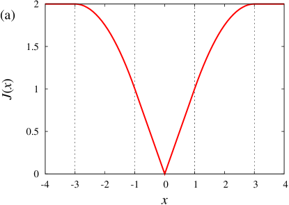
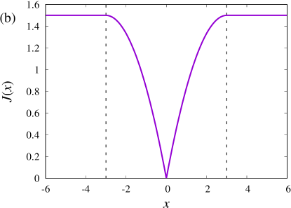
Figure 1: Shapes of (a) SCAD for $\lambda=1$ and $a=3$ and (b) MCP for $\lambda=1$ and $a=3$. The dashed lines represent the thresholds where penalty shape changes.

2.1 Estimator under SCAD and MCP

For understanding the properties of SCAD and MCP, let us consider the one-dimensional fitting problem of the input $w$ using Gaussian model penalized by SCAD or MCP as

$$\hat{x}(s,w)=\arg\min_{x}\left\{\frac{x^{2}}{2s}-wx+J(x;\lambda,a)\right\},$$ (8)

where $s>0$. Both of SCAD and MCP have upward convex terms, hence to define a solution of (8) for all $w$ region, we need to carefully consider the possible region of $s$ and $a$, which give the coefficient of the quadratic term in R.H.S. of (8). In case of SCAD, the relationship $a>1+s$ should hold to obtain the solution as

$$\hat{x}(s,w)=\Sigma_{\mathrm{SCAD}}(s,w){\cal M}_{\mathrm{SCAD}}(s,w)$$ (9)

where ${\cal M}_{\mathrm{SCAD}}$ and $\Sigma_{\mathrm{SCAD}}$ represent the coefficients of linear and quadratic term in (8) given by

$${\cal M}_{\mathrm{SCAD}}(s,w) =\left\{\begin{array}[]{ll}w-\mathrm{sgn}(w)\lambda&\mathrm{for}~{}\lambda(1+s^{-1})\geq|w|>\lambda\\ w-\mathrm{sgn}(w)\frac{a\lambda}{a-1}&\mathrm{for}~{}a\lambda s^{-1}\geq|w|>\lambda(1+s^{-1})\\ w&\mathrm{for}~{}|w|>a\lambda s^{-1}\\ 0&\mathrm{otherwise}\end{array}\right.,$$ (14)

$$\Sigma_{\mathrm{SCAD}}(s,w) =\left\{\begin{array}[]{ll}s&\mathrm{for}~{}\lambda(1+s^{-1})\geq|w|>\lambda\\ \left(s^{-1}-\frac{1}{a-1}\right)^{-1}&\mathrm{for}~{}a\lambda s^{-1}\geq|w|>\lambda(1+s^{-1})\\ s&\mathrm{for}~{}|w|>a\lambda s^{-1}\\ 0&\mathrm{otherwise}\end{array}\right.,$$ (19)

and $\mathrm{sgn}(w)$ denotes the sign of $w$. An example of the estimator as a function of the input $w$ under SCAD is shown in Figure 2 (b), where $s=1$, $\lambda=1$ and $a=3$. The SCAD estimator behaves like the $\ell_{1}$ estimator, which is shown in Figure 2 (a), and like the ordinary least square (OLS) estimator when $\lambda(1+s^{-1})\geq|z|>\lambda$ and $|w|>a\lambda s^{-1}$, respectively. In the region $a\lambda s^{-1}\geq|w|>\lambda(1+s^{-1})$, the estimator linearly transits between $\ell_{1}$ and OLS estimators.

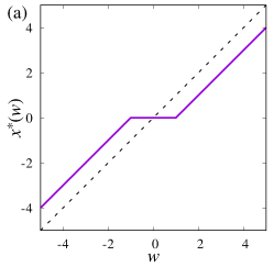
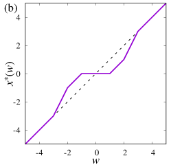
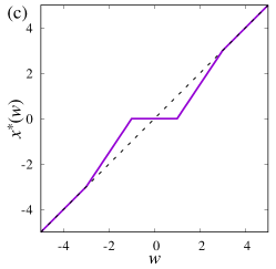
Figure 2: Behaviour of the estimator for (a) $\ell_{1}$, (b) SCAD, and (c) MCP. The dashed diagonal lines represent OLS estimator.

From the same argument as SCAD, $a>s$ should hold to define the solution of (8) under MCP. Further, the condition $a>1$ is imposed in the definition of MCP, hence in summarize the restriction is given as $a>\min\{1,s\}$. When the condition $a>\min\{1,s\}$ is satisfied, the solution of the single body problem under MCP is given by [18]

$$x^{*}(s,w)=\Sigma_{\mathrm{MCP}}(s,w){\cal M}_{\mathrm{MCP}}(s,w),$$ (20)

where

$${\cal M}_{\mathrm{MCP}}(s,w) =\left\{\begin{array}[]{ll}w-\mathrm{sgn}(w)\lambda&\mathrm{for}~{}a\lambda s^{-1}\geq|w|>\lambda\\ w&\mathrm{for}~{}|w|>a\lambda s^{-1}\\ 0&\mathrm{otherwise}\end{array}\right.,$$ (24)

$$\Sigma_{\mathrm{MCP}}(s,w) =\left\{\begin{array}[]{ll}(s^{-1}-a^{-1})^{-1}&\mathrm{for}~{}a\lambda s^{-1}\geq|w|>\lambda\\ s&\mathrm{for}~{}|w|>a\lambda s^{-1}\\ 0&\mathrm{otherwise}\end{array}\right..$$ (28)

Figure 2 (c) shows the behaviour of the MCP estimator at $s=1$, $\lambda=1$, and $a=3$. The MCP estimator behaves like the OLS estimator at $|w|>a\lambda s^{-1}$, and is connected from zero to the OLS estimator in the region $a\lambda s^{-1}\geq|w|>\lambda$.

3 Replica analysis for SCAD and MCP

We assume that the signal to be reconstructed is generated according to the Bernoulli–Gaussian distribution,

$$P_{0}(\bm{x}^{0})=\prod_{i}\left\{(1-\rho)\delta(x_{i}^{0})+\frac{\rho}{\sqrt{2\pi\sigma_{x}^{2}}}\exp\left(-\frac{(x_{i}^{0})^{2}}{2\sigma_{x}^{2}}\right)\right\},$$ (29)

where $\delta(x)$ is the Dirac delta function. Further, we consider the measurement matrix $A$ to be a random Gaussian, where each component is independently and identically distributed according to the Gaussian distribution with mean 0 and variance $N^{-1}$. The measurement is expressed as $\bm{y}=A\bm{x}^{0}$, and the minimization of $J(\bm{x};\lambda,a)$ is implemented under the constraint $\bm{y}=A\bm{x}$. For mathematical tractability, we express the constraint $\bm{y}=A\bm{x}$ by introducing a parameter $\tau$ as

$$P_{\tau}(\bm{y}|\bm{x})=\frac{1}{(\sqrt{2\pi\tau})^{M}}\exp\left\{-\frac{1}{2\tau}||\bm{y}-A\bm{x}||_{2}^{2}\right\},$$ (30)

where the probability is concentrated at $\bm{y}=A\bm{x}$ taking the limit $\tau\to 0$. The posterior distribution corresponding to the problem (3) is given by

$$P(\bm{x}|\bm{y})=\lim_{\beta\to\infty}\lim_{\tau\to 0}\frac{1}{Z_{\beta,\tau}(\bm{y})}\exp(-\beta J(\bm{x};\lambda,a))P_{\tau}(\bm{y}|\bm{x}),$$ (31)

where $\beta$ is a parameter to attain the uniform distribution over the minimizer of (3) at $\beta\to\infty$, and

$$Z_{\beta,\tau}(\bm{y})=\int d\bm{x}\exp(-\beta J(\bm{x};\lambda,a))P_{\tau}(\bm{y}|\bm{x})$$ (32)

is the normalization constant. The minimizer of (3) is given by $\hat{\bm{x}}=\langle\bm{x}\rangle$, where $\langle\cdot\rangle$ denotes the expectation with respect to $\bm{x}$ according to the posterior distribution (31).

The performance of the reconstruction (3) depends on the randomness $A$ and $\bm{x}^{0}$. Here, we examine the typical performance of the SCAD and MCP minimization at $N\to\infty$ and $M\to\infty$ keeping $M/N=\alpha\sim O(1)$, where $\alpha$ is the compression ratio. Free energy density defined by

$$f=-\lim_{\beta\to\infty}\lim_{N\to\infty}\lim_{\tau\to 0}\frac{1}{N\beta}E_{\bm{x^{0}},A}[\ln Z_{\beta,\tau}(\bm{y})]$$ (33)

is the key in this discussion, where $E_{\bm{x}^{0},A}[\cdots]$ denotes the expectation with respect to $A$ and $\bm{x}^{0}$ introduced for the discussion of the typical property. Here, we proceed the calculation for general $\tau$ and $\beta$, and take the limit after the derivation of the general form. It is calculated using the following identity

$$E_{\bm{x}^{0},A}[\ln Z_{\beta,\tau}(\bm{y})]=\lim_{n\to 0}\frac{E_{\bm{x}^{0},A}[Z^{n}_{\beta,\tau}(\bm{y})]-1}{n}.$$ (34)

Assuming that $n$ is a positive integer, we can express the expectation of $Z_{\beta}^{n}$ in (34) using $n$-replicated systems

$$E_{\bm{x}^{0},A}[Z_{\beta,\tau}^{n}(\bm{y})] =\int dAd\bm{y}d\bm{x}^{0}P_{0}(\bm{x}^{0})P_{A}(A)\delta(\bm{y}-A\bm{x}^{0})$$ (35)

$$\times\int d\bm{x}^{(1)}\cdots d\bm{x}^{(n)}\lim_{\tau\to 0}\frac{1}{(\sqrt{2\pi\tau})^{nM}}$$

$$\times\exp\Big{[}\sum_{a=1}^{n}\Big{\{}-\frac{1}{2\tau}||\bm{y}-A\bm{x}^{(a)}||_{2}^{2}-\beta J(\bm{x}^{(a)};\lambda,a)\Big{\}}\Big{]}.$$

The detail of the calculation is shown in [19, 13, 16], and here we briefly summarize the calculation. The free energy density under the RS assumption is given by

$$f=\mathrm{extr}_{\Omega,\tilde{\Omega}}\left[\frac{\alpha(Q-2m+\rho\sigma_{x}^{2})}{2\chi}+m\tilde{m}-\frac{\tilde{Q}Q-\tilde{\chi}\chi}{2}+\frac{\overline{\xi(\tilde{Q},\sigma)}}{2}\right],$$ (36)

where $\mathrm{extr}_{\Omega,\tilde{\Omega}}$ represents the extremization with respect to the quantities $\Omega=\{Q,\chi,m\}$ and $\tilde{\Omega}=\{\tilde{Q},\tilde{\chi},\tilde{m}\}$. The function $\xi(\tilde{Q},\sigma)$ depends on the regularization as

$$\xi(\tilde{Q},\sigma) =2\int DzL(\tilde{Q},\sigma z),$$ (37)

$$L(\tilde{Q},\sigma z) =\min_{x}\Big{(}\frac{\tilde{Q}}{2}x^{2}-\sigma zx+J(x;\lambda,a)\Big{)},$$ (38)

where $\int Dz=\int_{-\infty}^{\infty}dz\exp(-z^{2}/2)/\sqrt{2\pi}$. Equation (38) is equivalent to the one-dimensional problem (8). Here, $\overline{\cdots}$ denotes the average over $\sigma$ according to the distribution

$$P_{\sigma}(\sigma)=(1-\rho)\delta(\sigma-\sigma_{-})+\rho\delta(\sigma-\sigma_{+}),$$ (39)

with $\sigma_{-}=\sqrt{\tilde{\chi}}$ and $\sigma_{+}=\sqrt{\tilde{\chi}+\tilde{m}^{2}\sigma_{x}^{2}}$. The random fields $\sigma_{-}z$ and $\sigma_{+}z$ effectively represents the randomness induced by $A$ and $\bm{x}^{0}$, in particular zero-signals and non-zero-signals, respectively. We denote the solution of $x$ in the effective single-body problem (38) as $x^{*}(\tilde{Q}^{-1},\sigma z)$, which depends on the regularization, and we consider the specific form of $x^{*}(\tilde{Q}^{-1},\sigma z)$ and $L(\tilde{Q},\sigma z)$ later. The saddle point equations are given by

$$\chi =-\frac{\partial\overline{\xi(\tilde{Q},\sigma)}}{\partial\tilde{\chi}}=\int Dz\overline{\frac{\partial x^{*}(\tilde{Q}^{-1},\sigma z)}{\partial(\sigma z)}},$$ (40)

$$Q =\frac{\partial\overline{\xi(\tilde{Q},\sigma)}}{\partial\tilde{Q}}=\int Dz\overline{(x^{*}(\tilde{Q}^{-1},\sigma z))^{2}},$$ (41)

$$m =-\frac{1}{2}\frac{\partial\overline{\xi(\tilde{Q},\sigma)}}{\partial\tilde{m}}={\rho\tilde{m}\sigma_{x}^{2}}\int Dz\frac{\partial x^{*}(\tilde{Q}^{-1},\sigma_{+}z)}{\partial(\sigma_{+}z)},$$ (42)

$$\tilde{\chi} =\frac{\alpha(Q-2m+\rho\sigma_{x}^{2})}{\chi^{2}},$$ (43)

$$\tilde{Q} =\frac{\alpha}{\chi},$$ (44)

$$\tilde{m} =\frac{\alpha}{\chi}.$$ (45)

At the saddle point, $x^{*}(\tilde{Q}^{-1},\sigma z)$ is statistically equivalent to the point estimate $\hat{\bm{x}}$, and $\chi,Q$ and $m$ are related to the physical quantities as

$$Q =\lim_{N\to\infty}\frac{1}{N}\sum_{i=1}^{N}E_{\bm{x}^{0},A}[\hat{x}_{i}^{2}],$$ (46)

$$m =\lim_{N\to\infty}\frac{1}{N}\sum_{i=1}^{N}E_{\bm{x}^{0},A}[x_{i}^{0}\hat{x}_{i}],$$ (47)

$$\chi =\lim_{\beta\to\infty}\lim_{N\to\infty}\frac{\beta}{N}\sum_{i=1}^{N}E_{\bm{x}^{0},A}\left[\langle x_{i}^{2}\rangle-\langle x_{i}\rangle^{2}\right].$$ (48)

Hence, the expectation value of the mean squared error (MSE) between the reconstructed signal and the original signal is represented as

$$\varepsilon\equiv\frac{1}{N}E_{\bm{x}^{0},A}\left[||\hat{\bm{x}}-\bm{x}^{0}||_{2}^{2}\right]=Q-2m+\rho\sigma_{x}^{2}.$$ (49)

The saddle point equations for variables $\Omega=\{Q,\chi,m\}$ directly depend on the functional form of the regularization, but the equations for $\tilde{\Omega}$ do not depend on it. In the following subsections, we show the form of saddle point equations of $\Omega$ for SCAD and MCP.

The RS solution is stable against the symmetry breaking perturbation when [13, 16]

$$\frac{\alpha}{\chi^{2}}\int Dz\overline{\left(\frac{\partial x^{*}(\tilde{Q}^{-1},\sigma z)}{\partial(\sigma z)}\right)^{2}}<1,$$ (50)

which is known as de Almeida–Thouless (AT) condition [20]. The form of this condition also depends on the functional form of the regularization.

3.1 SCAD

As mentioned in Sec.2.1, $\tilde{Q}>(a-1)^{-1}$ should hold to define the minimizer of (38). In the following, the subspace of the macroscopic parameters where the minimizer of (38) can be defined is denoted by $\Omega^{\dagger}(a)\equiv\{Q,\chi,m|\tilde{Q}>(a-1)^{-1}\}$ for each $a$, and we restrict our discussion to $\Omega^{\dagger}(a)$. When we are in $\Omega^{\dagger}(a)$, the minimizer of (38) under SCAD is given by [18]

$$x^{*}(\tilde{Q}^{-1},\sigma z)=\Sigma_{\mathrm{SCAD}}(\tilde{Q}^{-1},\sigma z){\cal M}_{\mathrm{SCAD}}(\tilde{Q}^{-1},\sigma z),$$ (51)

and substituting the solution (51) into (38), we obtain

$$-2L(\tilde{Q},\sigma z)=\left\{\begin{array}[]{ll}\displaystyle\frac{(\sigma z-\lambda{\rm sgn}(z))^{2}}{\tilde{Q}}&(\sqrt{2}\theta_{1}(\sigma)<|z|\leq\sqrt{2}\theta_{2}(\sigma))\\ \displaystyle\frac{(\sigma z-\frac{a\lambda}{a-1})^{2}}{\tilde{Q}-\frac{1}{a-1}}+\frac{\lambda^{2}}{a-1}&(\sqrt{2}\theta_{2}(\sigma)<|z|\leq\sqrt{2}\theta_{3}(\sigma))\\ \displaystyle\frac{(\sigma z)^{2}}{\tilde{Q}}-(a+1)\lambda^{2}&(|z|>\sqrt{2}\theta_{3}(\sigma))\\ 0&({\rm otherwise})\end{array}\right.,$$ (52)

where $\theta_{1}(\sigma)={\lambda}/(\sqrt{2}\sigma)$, $\theta_{2}(\sigma)=\lambda(1+\tilde{Q})/(\sqrt{2}\sigma)$, and $\theta_{3}(\sigma)=a\lambda\tilde{Q}/(\sqrt{2}\sigma)$. Equation (37) for SCAD regularization is derived as

$$-\xi(\sigma)=\xi_{1}(\sigma)+\xi_{2}(\sigma)+\xi_{3}(\sigma)+\frac{\lambda^{2}\xi_{4}(\sigma)}{a-1}-(a+1)\lambda^{2}\mathrm{erfc}(\theta_{3}(\sigma)),$$ (53)

where

$$\xi_{1}(\sigma) =\frac{\sigma^{2}}{\tilde{Q}}\Big{[}-\frac{2\theta_{1}(\sigma)}{\sqrt{\pi}}\Big{(}e^{-\theta_{1}^{2}(\sigma)}+(\tilde{Q}-1)e^{-\theta_{2}^{2}(\sigma)}\Big{)}$$ (54)

$$+(1+2\theta_{1}^{2}(\sigma))\{\mathrm{erfc}(\theta_{1}(\sigma))-{\rm erfc}(\theta_{2}(\sigma))\}\Big{]},$$

$$\xi_{2}(\sigma) =\frac{\sigma^{2}}{\tilde{Q}-\frac{1}{a-1}}\Big{[}\frac{2}{\sqrt{\pi}}\Big{\{}\theta_{2}(\sigma)e^{-\theta_{2}^{2}(\sigma)}$$ (55)

$$-\theta_{3}(\sigma)e^{-\theta_{3}^{2}(\sigma)}-\frac{2\theta_{3}(\sigma)}{\tilde{Q}(a-1)}\left(e^{-\theta_{2}^{2}(\sigma)}-e^{-\theta_{3}^{2}(\sigma)}\right)\Big{\}}$$

$$+\Big{\{}1+2\Big{(}\frac{\theta_{3}(\sigma)}{\tilde{Q}(a-1)}\Big{)}^{2}\Big{\}}\xi_{4}(\sigma)\Big{]},$$

$$\xi_{3}(\sigma) =\frac{\sigma^{2}}{\tilde{Q}}\Big{[}\frac{2\theta_{3}(\sigma)}{\sqrt{\pi}}e^{-\theta_{3}^{2}(\sigma)}+{\rm erfc}(\theta_{3}(\sigma))\Big{]},$$ (56)

$$\xi_{4}(\sigma) ={\rm erfc}(\theta_{2}(\sigma))-{\rm erfc}(\theta_{3}(\sigma)).$$ (57)

The regularization-dependent saddle point equations are given by

$$Q =\overline{\frac{\xi_{1}(\sigma)}{\tilde{Q}}+\frac{\xi_{2}(\sigma)}{\tilde{Q}-\frac{1}{a-1}}+\frac{\xi_{3}(\sigma)}{\tilde{Q}}},$$ (58)

$$\chi =\frac{1}{\tilde{Q}}\Big{[}\hat{\rho}+\frac{\frac{1}{a-1}}{\tilde{Q}-\frac{1}{a-1}}\overline{\xi_{4}(\sigma)}\Big{]},$$ (59)

$$m ={\rho\sigma_{x}^{2}}\left[\mathrm{erfc}(\theta_{1}(\sigma_{+}))+\frac{\frac{1}{a-1}\xi_{4}(\sigma_{+})}{\tilde{Q}-\frac{1}{a-1}}\right],$$ (60)

where $\hat{\rho}$ is the density of the nonzero component in the estimate given by

$$\hat{\rho}=\overline{\mathrm{erfc}(\theta_{1}(\sigma))}.$$ (61)

From (50), the AT condition is derived as

$$\frac{1}{\alpha}\left[\hat{\rho}+\left\{\left(\frac{\tilde{Q}}{\tilde{Q}\!-\!\frac{1}{a-1}}\right)^{2}-1\right\}\overline{\xi_{4}(\sigma)}\right]<1.$$ (62)

3.2 MCP

As with SCAD, we concentrate our discussion on the subspace of the macroscopic parameters $\Omega^{\dagger}(a)=\{Q,\chi,m|\tilde{Q}>a^{-1}\}$, where the solution of (38) can be defined. The solution of the single body problem under MCP in $\Omega^{\dagger}(a)=\{Q,\chi,m|\tilde{Q}>a^{-1}\}$ is given by [18]

$$x^{*}(\tilde{Q}^{-1},\sigma z)=\Sigma_{\mathrm{MCP}}(\tilde{Q}^{-1},\sigma z){\cal M}_{\mathrm{MCP}}(\tilde{Q}^{-1},\sigma z),$$ (63)

and we obtain

$$-2L(\tilde{Q},\sigma)=\left\{\begin{array}[]{ll}\displaystyle\frac{(\sigma z-{\lambda{\rm sgn}(z))^{2}}}{\tilde{Q}-a^{-1}}&(\sqrt{2}\theta_{1}(\sigma)<|z|\leq\sqrt{2}\theta_{2}(\sigma))\\ \displaystyle\frac{(\sigma z)^{2}}{\tilde{Q}}-\lambda a^{2}&(|z|>\sqrt{2}\theta_{2}(\sigma))\\ 0&({\rm otherwise})\end{array}\right.,$$ (64)

where $\theta_{1}(\sigma)=\lambda/(\sqrt{2}\sigma)$ and $\theta_{2}(\sigma)=a\lambda\tilde{Q}/(\sqrt{2}\sigma)$ , and (37) for MCP is derived as

$$-\xi(\sigma)=\xi_{1}(\sigma)+\xi_{2}(\sigma),$$ (65)

where

$$\xi_{1}(\sigma) =-\frac{2\sigma^{2}}{\sqrt{\pi}(\tilde{Q}-a^{-1})}\left\{\theta_{1}(\sigma)(e^{-\theta_{1}^{2}(\sigma)}-e^{-\theta_{2}^{2}(\sigma)})-e^{-\theta_{2}^{2}(\sigma)}(\theta_{1}(\sigma)-\theta_{2}(\sigma))\right\}$$ (66)

$$+\frac{(\sigma^{2}+\lambda^{2})\xi_{3}(\sigma)}{\tilde{Q}-a^{-1}},$$

$$\xi_{2}(\sigma) =\frac{\sigma^{2}}{\tilde{Q}}\left(\frac{2\theta_{2}(\sigma)}{\sqrt{\pi}}e^{-\theta_{2}^{2}(\sigma)}+{\rm erfc}(\theta_{2}(\sigma))\right)-\lambda a^{2}{\rm erfc}(\theta_{2}(\sigma)),$$ (67)

$$\xi_{3}(\sigma) ={\rm erfc}(\theta_{1}(\sigma))-{\rm erfc}(\theta_{2}(\sigma)).$$ (68)

The saddle point equations for $\Omega$ are given by

$$Q =\overline{\frac{\xi_{1}(\sigma)}{\tilde{Q}-\frac{1}{a}}+\frac{\sigma^{2}}{\tilde{Q}^{2}}\left\{\frac{2\theta_{2}(\sigma)}{\sqrt{\pi}}e^{-\theta_{2}^{2}(\sigma)}+{\rm erfc}(\theta_{2}(\sigma))\right\}},$$ (69)

$$\chi =\frac{1}{\tilde{Q}}\left[\hat{\rho}+\frac{a^{-1}\overline{\xi_{3}(\sigma)}}{\tilde{Q}-a^{-1}}\right],$$ (70)

$$m =\rho\sigma_{x}^{2}\left[\mathrm{erfc}(\theta_{1}(\sigma_{+}))+\frac{a^{-1}\xi_{3}(\sigma_{+})}{\tilde{Q}-a^{-1}}\right],$$ (71)

where $\hat{\rho}$ is the density of nonzero component in the estimate given by

$$\hat{\rho}=\overline{{\rm erfc}(\theta_{1}(\sigma))}.$$ (72)

The AT condition for MCP is derived as

$$\frac{1}{\alpha}\left[\hat{\rho}+\left\{\left(\frac{\tilde{Q}}{\tilde{Q}-a^{-1}}\right)^{2}-1\right\}\overline{\xi_{3}(\sigma)}\right]<1.$$

4 Stability of success solution

One of the solutions of the saddle point equations in $\Omega^{\dagger}(a)$ is characterized by $Q=m=\rho\sigma_{x}^{2}$. Following the correspondence between the order parameters and the MSE (49), this solution indicates the perfect reconstruction of the original signal $\bm{x}^{0}$. Hence, we call the solution with $Q=m=\rho\sigma_{x}^{2}$ the success solution. The saddle point equation can have solutions other than the success solution; however, these solutions do not satisfy the AT condition as far as we observed. Substituting the relationship $Q=m=\rho\sigma_{x}^{2}$, we immediately obtain $\chi=0$ and $\tilde{Q}=\tilde{m}=\infty$, and the only variable to be solved is $\tilde{\chi}$. The expansion of $Q$ and $m$ up to the order $O(\tilde{Q}^{-2})$ gives the expression of $\tilde{\chi}$ for the success solution under SCAD

$$\tilde{\chi} =\frac{1-\rho}{\alpha}\left[-\frac{2\tilde{\chi}}{\sqrt{\pi}}\theta_{-}e^{-\theta_{-}^{2}}+(\tilde{\chi}+\lambda^{2})\mathrm{erfc}(\theta_{-})\right]$$ (74)

$$+\frac{\rho}{\alpha}\Big{[}\tilde{\chi}+\lambda^{2}\left\{1-\mathrm{erfc}(\theta_{+})\right\}+\left\{\left(\frac{a\lambda}{a-1}\right)^{2}+\frac{\sigma_{x}^{2}}{(a-1)^{2}}\right\}\{\mathrm{erfc}(\theta_{+})-\mathrm{erfc}(a\theta_{+})\}$$

$$+\frac{2\sigma_{x}^{2}\theta_{+}}{\sqrt{\pi}(a-1)}\left\{\frac{a}{a-1}(e^{-a^{2}\theta_{+}^{2}}-e^{-\theta_{+}^{2}})-e^{-\theta_{+}^{2}}\right\}\Big{]},$$

and under MCP

$$\tilde{\chi} =\frac{1-\rho}{\alpha}\left\{-\frac{2\tilde{\chi}}{\sqrt{\pi}}\theta_{-}e^{-\theta_{-}^{2}}+(\tilde{\chi}+\lambda^{2})\mathrm{erfc}(\theta_{-})\right\}$$ (75)

$$+\frac{\rho}{\alpha}\left[\tilde{\chi}+\left(\lambda^{2}+\frac{\sigma_{x}^{2}}{a^{2}}\right)\left(1-\mathrm{erfc}(a\theta_{+})\right)+\frac{2\sigma_{x}^{2}\theta_{+}}{a\sqrt{\pi}}e^{-a^{2}\theta_{+}^{2}}-\frac{4\sigma_{x}^{2}\theta_{+}}{a\sqrt{\pi}}\right],$$

where $\theta_{-}=\lambda/\sqrt{2\tilde{\chi}}$ and $\theta_{+}=\lambda/\sqrt{2\sigma_{x}^{2}}$. Eqs. (74) and (75) are reduced to the saddle point equation of $\tilde{\chi}$ corresponding to the success solution for $\ell_{1}$ regularization by setting $\lambda=1$ and when $a\to\infty$ [16].

For both the penalties, the success solution is a locally stable solution as a saddle point of the RS free energy when

$$\frac{1}{\alpha}\left\{(1-\rho)\mathrm{erfc}\left(\theta_{-}\right)+\rho\right\}<1.$$ (76)

This condition is derived by the linear stability analysis of $\chi$ around 0. Further, we can show that the AT condition for the success solution is equivalent to (76). This means that when the success solution is locally stable as a RS saddle point, it is also stable with respect to the replica symmetry breaking perturbation. Therefore, the reconstruction limit $\alpha_{c}(\rho)$ is defined as the minimum value of $\alpha$ that satisfies (76) for each $\rho$. We also define $\rho_{c}(\alpha)$ as the maximum value of $\rho$ to satisfy (76) at $\alpha$, and we use both $\alpha_{c}(\rho)$ and $\rho_{c}(\alpha)$ for convenience.

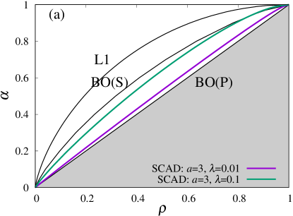
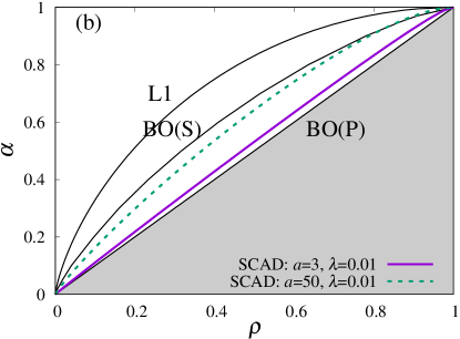
Figure 3: Reconstruction limit of SCAD at (a) $a=3$ for $\lambda=0.01$ and $\lambda=0.1$ and (b) $\lambda=0.01$ $a=3$ and $a=50$. The lines with ‘L1’, ‘BO(S)’ and ‘BO(P)’ are the reconstruction limit under $\ell_{1}$ minimization, the algorithmic limit by the Bayes-optimal method given by spinodal transition, and the phase transition point of the Bayes-optimal method, respectively. The shaded regions are $\alpha<\rho$.

Figs. 3 and 4 show the $\rho$-dependence of $\alpha_{c}(\rho)$ for SCAD minimization and MCP minimization, respectively, where (a)s represent $a=3$ and (b)s represent $\lambda=0.01$. The typical reconstruction is possible in the parameter region $\alpha\geq\alpha_{c}(\rho)$, and that for $\ell_{1}$ minimization (L1) and the algorithmic limit of the Bayes-optimal method given by spinodal transition (BO(S)), and the phase transition boundary of the Bayes-optimal method (BO(P)) over which the success solution is locally stable, are shown for comparison. As $\lambda$ and $a$ decrease, $\alpha_{c}(\rho)$ of SCAD and MCP become less than that of the algorithmic limit of the Bayes-optimal reconstruction method [17]. Further, the reconstruction limit $\alpha_{c}(\rho)$ approaches $\rho$ as $\lambda\to 0$. Mathematically, $\alpha_{c}(\rho)\to\rho$ is provided by scaling $\theta_{-}\to\infty$ and $\tilde{\chi}\to 0$ at $\lambda\to 0$, which reduces (76) to $\rho<\alpha$. This inequality, $\rho<\alpha$, is considered to be the fundamental limit, because in general sparse estimation methods, the estimation of the support increases the effective degrees of the estimated variables. Hence, we need more measurements than the number of the variables to be estimated. It is indicated that SCAD and MCP with $\lambda\to 0$ achieve the typical reconstruction when the number of the measurements and that of nonzero variables are balanced.

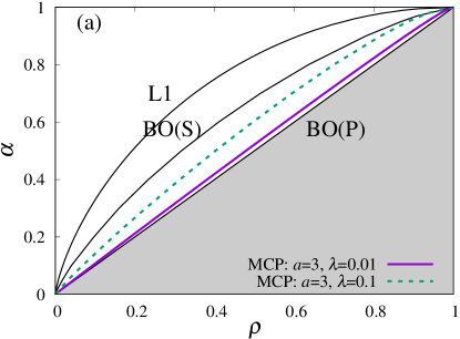
Figure 4: Reconstruction limit of MCP at (a) $a=3$ for $\lambda=0.01$ and $\lambda=0.1$ and (b) $\lambda=0.01$ for $a=3$ and $a=50$. The lines with ‘L1’, ‘BO(S)’ and ‘BO(P)’ are the same as Figure 3. The shaded regions are $\alpha<\rho$.

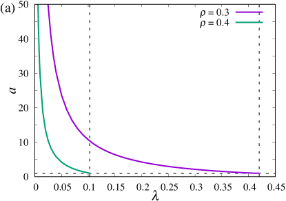
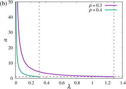
Figure 5: Reconstruction limit $a_{c}(\lambda)$ at $\alpha=0.5$ for (a) SCAD and (b) MCP, respectively. The vertical dashed lines represent the maximum value of $\lambda$, where the reconstruction is possible with $a_{\min}<a\leq a_{c}(\lambda)$. The horizontal dashed lines represent $a=1$, which is the minimum value of $a$ for the success solution.

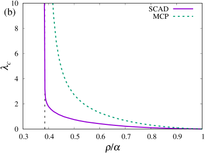
Figure 6: $\rho/\alpha$-dependence of $\lambda_{c}$ for (a) $\alpha=0.3$ and (b) $\alpha=0.5$. In the parameter region on the left side to the vertical lines, $\ell_{1}$ minimization reconstructs the original signals.

We denote as $a_{c}(\lambda)$ the value of $a$ under which the signals can be reconstructed for each $\lambda$. The reconstruction limit $a_{c}(\lambda)$ on the $\lambda-a$ plane is shown in Figure 5 for (a) SCAD and (b) MCP, respectively, at $\alpha=0.5$ for $\rho=0.3$ and $\rho=0.4$. The horizontal dashed lines represent $a_{\min}$, which is equal to 1 when the success solution is stable, and the signals can be reconstructed in the parameter region $a_{\min}<a\leq a_{c}(\lambda)$. The dashed vertical lines represent $\lambda_{c}$, defined as the maximum value of $\lambda$ that gives $a_{c}(\lambda)>a_{\min}$. Hence, the signal cannot be reconstructed at $\lambda\geq\lambda_{c}$. For the reconstruction of dense signals, small nonconvexity parameters $\lambda$ and $a$ are required, and $a_{c}(\lambda)$ and $\lambda_{c}$ for MCP are always greater than that for SCAD. The dependence of $\lambda_{c}$ on $\rho/\alpha$ for SCAD and MCP are compared in Figure 6 for (a) $\alpha=0.3$ and (b) $\alpha=0.5$. The vertical lines represent the reconstruction limit of $\ell_{1}$ minimization, and the values of $\lambda_{c}$ diverge as $\rho/\alpha$ approaches the $\ell_{1}$ reconstruction limit. This divergence of $\lambda_{c}$ means that one can reconstruct the signals using any $\lambda\in(0,\infty)$ and $a\in(a_{\min},\infty)$ when the signals are sufficiently sparse to be reconstructed by $\ell_{1}$ minimization. For any system parameters, the divergence of $\lambda_{c}$ in MCP is faster than that in SCAD, which indicates that the range of possible values of nonconvexity parameters for reconstruction in MCP is wider than that in SCAD. In this sense, MCP is superior to SCAD.

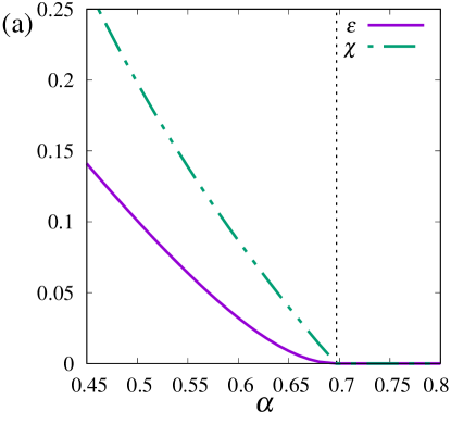
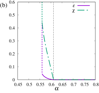
Figure 7: $\alpha$-dependence of $\varepsilon$ and $\chi$ in RS solution of SCAD at $\rho=0.35$ for (a) $\lambda=1,~{}a=10$ and (b) $\lambda=0.3,~{}a=5$. The vertical dotted lines indicate $\alpha_{c}$, and the vertical dashed lines in (b) indicate the disappearance of the finite $\varepsilon$ and $\chi$.

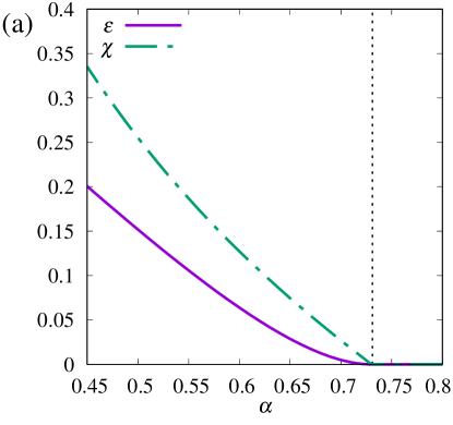
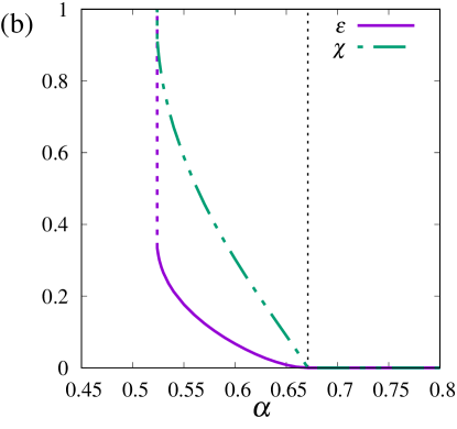
Figure 8: $\alpha$-dependence of $\varepsilon$ and $\chi$ in RS solution of MCP at $\rho=0.4$ for (a) $\lambda=1,~{}a=10$ and (b) $\lambda=0.5,~{}a=5$. The vertical dotted lines indicate $\alpha_{c}$, and the vertical dashed lines in (b) indicate the disappearance of the finite $\varepsilon$ and $\chi$.

4.1 Comment on the RS-failure solution

We mention the existence of the solution of RS saddle point equation at $\alpha<\alpha_{c}$ for subsequent discussions. One can find a solution with $\varepsilon>0$ ($Q<\rho\sigma_{x}^{2}$ and $m<\rho\sigma_{x}^{2}$) and $\chi>0$ within $\Omega^{\dagger}(a)$ at $\alpha<\alpha_{c}$, which violates the AT condition. We term this solution as RS-unstable failure solution. Figs. 7 and 8 show $\alpha$-dependence of $\varepsilon$ and $\chi$ for SCAD and MCP, respectively, where the vertical dashed lines represent $\alpha_{c}$. The RS-unstable failure solution is smoothly connected to the success solution that appears at $\alpha\geq\alpha_{c}$, and do not coexist with the success solution. The RS-unstable failure solution does not contribute to the equilibrium property of the system, but this solution is still useful to consider the behavior of the algorithm as shown in the following sections.

4.2 Comment on the diverging “solution”

As shown in Figs. 7 (b) and 8 (b), when $\lambda$ is sufficiently small, the values of $\varepsilon$ and $\chi$ tend to diverge at sufficiently small $\alpha$, and the solution with finite $\varepsilon$ and $\chi$ disappears. In fact, (59) indicates that the solution $\chi\to\infty$ is stable for both SCAD and MCP when

$$\alpha<(1-\rho)\mathrm{erfc}(\theta_{\infty}^{-})+\rho\mathrm{erfc}(\theta_{\infty}^{+})$$ (77)

holds, where $\theta_{\infty}^{+}=a\lambda\sqrt{\alpha/\{2(\alpha+\varepsilon)\}}$ and $\theta_{\infty}^{-}=a\lambda\sqrt{\alpha/(2\varepsilon)}$, although the solution is out of the physical region $\Omega^{\dagger}(a)$. Considering the limit $\chi\to\infty$, the set of the saddle point equations for SCAD and MCP is reduced to the same one equation for the MSE $\varepsilon$ as

$$\varepsilon =\frac{\varepsilon(1-\rho)}{\alpha}\left\{\frac{2\theta_{\infty}^{-}}{\sqrt{\pi}}e^{-(\theta_{\infty}^{-})^{2}}+\mathrm{erfc}(\theta_{\infty}^{-})\right\}+\frac{\rho(\varepsilon+\alpha)}{\alpha}\left\{\frac{2\theta_{\infty}^{+}}{\sqrt{\pi}}e^{-(\theta_{\infty}^{+})^{2}}+\mathrm{erfc}(\theta_{\infty}^{+})\right\}$$ (78)

$$-2\rho\sigma_{x}^{2}\mathrm{erfc}(\theta_{\infty}^{+})+\rho\sigma_{x}^{2}.$$

The solutions of (78) and (LABEL:eq:varepsilon_MCP) can be finite or infinite depending on $\alpha$, $\lambda$, $\rho$ and $a$, and the infinite $\varepsilon$ is always stable if it exists when $\alpha<1$. The diverging solutions do not contribute to the thermodynamic behavior, because they are not in the region $\Omega^{\dagger}(a)$, but they affect the algorithmic behavior of SCAD or MCP minimization.

5 Approximate message passing with nonconvexity control

For numerical computation of the estimate under a given measurement matrix, AMP is a feasible algorithm with low computational cost. As discussed below, the typical trajectory and fixed point of AMP can be connected to the analysis based on replica method, hence we can understand algorithmic behavior by comparing with the analysis. The detailed derivation has been given by the previous studies [13, 17, 21], and here we briefly introduce the algorithm. In AMP, the estimates under a general separable sparse penalty is recursively updated as

$$\hat{x}_{i}^{(t+1)}=\arg\min_{x}\left\{\frac{\tilde{Q}_{i}^{(t)}}{2}x^{2}-h_{i}^{(t)}x+J(x_{i};\lambda,a)\right\},$$ (79)

where $\hat{x}_{i}^{(t)}$ denotes the estimate at time step $t$, and

$$\tilde{Q}_{i}^{(t)} =\frac{1}{\hat{V}^{(t)}},$$ (80)

$$h_{i}^{(t)} =\hat{x}_{i}^{(t-1)}\tilde{Q}_{i}^{(t)}+\sum_{\mu=1}^{M}A_{\mu i}R_{\mu}^{(t)},$$ (81)

$$\hat{V}^{(t)} =\frac{1}{M}\sum_{i=1}^{N}\hat{v}_{i}^{(t-1)},$$ (82)

$$\hat{v}_{i}^{(t)} =\frac{\partial\hat{x}_{i}^{(t)}}{\partial h_{i}^{(t)}},$$ (83)

$$R_{\mu}^{(t)} =\frac{y_{\mu}-\sum_{i}A_{\mu i}\hat{x}_{i}^{(t-1)}}{\hat{V}^{(t)}}.$$ (84)

The solution of (79) corresponds to the minimizer of (38), with the replacement of $\tilde{Q}$ and $\sigma z$ with $\tilde{Q}_{i}^{(t)}$ and $h_{i}^{(t)}$, respectively.

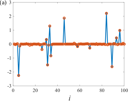
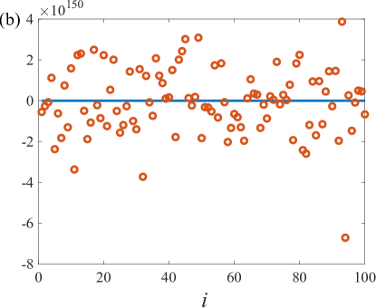
Figure 9: True signal $x_{i}^{0}$ (solid line) and reconstructed signal $\hat{x}_{i}$ (circles) at $N=100$ and $M=50$ for (a) $\rho=0.25$ with SCAD at $\lambda=1$ and $a=3$, and (b) $\rho=0.28$ with SCAD at $\lambda=0.1$ and $a=3$.

The local stability of AMP corresponds to the AT instability condition [13]. Hence, it is expected that AMP reconstructs the original signal in the theoretically derived parameter region $\alpha>\alpha_{c}(\rho)$ at sufficiently large $N$, because the current problem does not exhibit any first order transitions or spinodal transitions under fixed nonconvexity parameters, in contrast to the Bayes-optimal setting [17] or the Monte Carlo sampling case [22]. Figure 9 shows examples of reconstructed signals of $N=400$ and $\alpha=0.5$ after 1000 steps update of AMP under SCAD (a) at $\lambda=1$ and $a=3$ for $\rho=0.25$ and (b) at $\lambda=0.1$ and $a=3$ for $\rho=0.3$, where the original and reconstructed signals are represented by solid lines and circles, respectively. In these parameter regions, perfect reconstruction is theoretically supported, but as shown in Figure 9 (b), the naive update of AMP does not achieve the perfect reconstruction for small values of nonconvexity parameters. The discrepancy between the replica analysis and AMP appears, in particular, when the signal is dense. The tendency is common in both SCAD and AMP, hence we explain their characteristic behavior using SCAD as a representative.

As mentioned above, any other stable solutions do not exist when the success solution is locally stable, hence the discrepancy between the replica analysis and AMP cannot be understood by the spinodal transition as with the Bayes-optimal method. For understanding the difficulty in achieving the perfect reconstruction of the signal by AMP at a small nonconvexity parameter region, we use state evolution (SE) [23]. The typical trajectory of AMP is characterized by two parameters $V^{(t)}\equiv E_{\bm{x}^{0},A}[\hat{V}^{(t)}]$ and $\varepsilon^{(t)}\equiv E_{\bm{x}^{0},A}[\hat{\varepsilon}^{(t)}]$, where $\hat{\varepsilon}^{(t)}\equiv\sum_{i=1}^{N}(\hat{x}_{i}^{(t)}-x_{i}^{0})^{2}/N$ is the mean squared error at $t$-th iteration step. In particular, when the components of $A$ are independently and identically distributed with mean 0 and variance $1/N$, as for the Gaussian measurement matrix, the time evolution of $V^{(t)}$ and $\varepsilon^{(t)}$ is described by SE equations [13, 17]

$$V^{(t+1)} =\int dx^{0}P_{0}(x^{0})\int Dz\Sigma(\alpha^{-1}V^{(t)},x^{0}+z\sqrt{\alpha^{-1}\varepsilon^{(t)}}),$$ (85)

$$\varepsilon^{(t+1)} =\int dx^{0}P_{0}(x^{0})\int Dz\left[\hat{x}(\alpha^{-1}V^{(t)},x^{0}+z\sqrt{\alpha^{-1}\varepsilon^{(t)}})-x^{0}\right]^{2},$$ (86)

where $\hat{x}(s,w)=\Sigma_{\mathrm{p}}(s,w){\cal M}_{\mathrm{p}}(s,w)$ for $\mathrm{p}\in\{\mathrm{SCAD},\mathrm{MCP}\}$. SE is equivalent to the RS saddle point equation, and the fixed point denoted by $V^{*}$ and $\varepsilon^{*}$ correspond to the RS saddle point as $V^{*}=\chi$ and $\varepsilon^{*}=Q-2m+\rho\sigma_{x}^{2}$, respectively. Hence, the success solution is described as $V^{*}=\varepsilon^{*}=0$ in the SE. As mentioned in Sec. 4.1, the failure solution appears in some parameter regions, but it always involves the RS instability and never coexists with the success solution. Note that the flow of the SE describes the typical trajectory of the AMP with respect to $A$ and $\bm{x}^{0}$. Hence, it does not necessarily describe a trajectory under a fixed realization of $A$ and $\bm{x}^{0}$. However, it is expected that the trajectories converge to the flow of SE for a sufficiently large system size. Hence, SE flow supports an understanding of a trajectory of AMP under a fixed set of $A$ and $\bm{x}^{0}$ [24].

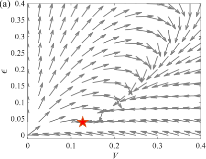
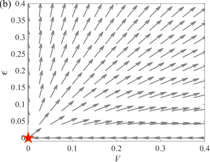
Figure 10: Flow of state evolution at $\alpha=0.5$ and $\rho=0.28$ for SCAD (a) $\lambda=1$ and $a=3$ and (b) $\lambda=0.1$ and $a=3$. The fixed points are depicted by stars.

Figure 10 shows the flow of SE at $\alpha=0.5$ and $\rho=0.28$ for SCAD at (a) $\lambda=1$ and $a=3$ and (b) $\lambda=0.1$ and $a=3$. The arrows assigned to the coordinate $(\hat{V},\hat{\varepsilon})$ is the normalized vector of $(V^{(t+1)}-V^{(t)},\varepsilon^{(t+1)}-\varepsilon^{(t)})$ with $V^{(t)}=\hat{V}$ and $\varepsilon^{(t)}=\hat{\varepsilon}$, which indicate the direction of SE’s flow, and the stars depict the fixed points of SE. As shown in Figure 10 (a), SE has a fixed point with finite $\varepsilon$ and $V$ for large $\lambda$, which corresponds to the RS-unstable failure solution, but as $\lambda$ decreases, most of the SE flow leads to a divergence of $V$ and $\varepsilon$ as shown in Figure 10(b); however, there is still a region close to the $V$-axis where the flows are directed to $V=\varepsilon=0$. This region shrinks to $V$-axis as the nonconvexity parameter decreases. Flows of SE in MCP is almost the same as SCAD shown in Figure 10. In case of $\ell_{1}$ minimization, one can check that SE reaches to the success solution from any initial condition of $(V,\varepsilon)$, namely the volume of the basin of attraction (BOA) diverges to infinity at $\alpha>\alpha_{c}(\rho)$ or $\rho<\rho_{c}(\alpha)$. Therefore, this shrinking basin and the diverging flow are significant properties of the minimization problems of SCAD and MCP.

We quantify the volume of the BOA under SCAD minimization and show its dependency on $\rho$ for $\alpha=0.5$ as Figure 11 (a). The BOA to $V=\varepsilon=0$ is zero at $\rho=\rho_{c}$, and gradually increases from zero as $\rho$ decreases from $\rho_{c}$. When the nonconvexity parameter $\lambda$ is small, the basin volume tends to be small for any $\rho$ region. Figure 11(b) shows the possible maximum value of $\varepsilon$, denoted by $\varepsilon_{\max}$, as an initial condition to converge to $V=\varepsilon=0$. Namely, $\varepsilon_{\max}$ is the maximum value of $\varepsilon$ on the boundary of the BOA. It means that to achieve perfect reconstruction at sufficiently large $\rho$ with small nonconvexity parameter, we need to set initial condition as $\varepsilon\sim O(10^{-2})$ for $\lambda=0.1$ and $a=3$, and as $\varepsilon\sim O(10^{-5})$ for $\lambda=0.01$ and $a=3$. Such initial conditions with small $\varepsilon$ is not realistic, and the possibility that AMP attains the success solution $V=\varepsilon=0$ from randomly chosen initial conditions is exceedingly small.

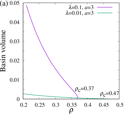
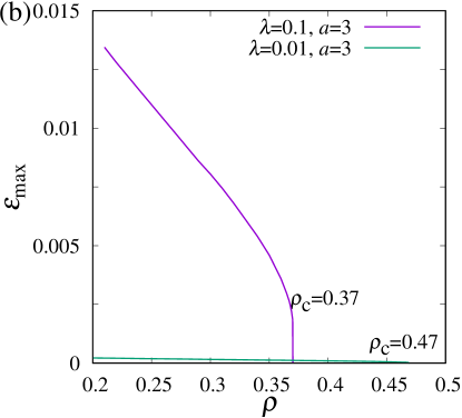
Figure 11: (a) Volume of the BOA to $V=\varepsilon=0$ at $\alpha=0.5$. (b) Maximum value of $\varepsilon$, denoted by $\varepsilon_{\max}$, on the boundary of the BOA.

The shrinking BOA is the origin of the difficulty of AMP for small nonconvexity parameters. To resolve this problem, we recall that the RS-unstable failure solution appears for $\alpha<\alpha_{c}$ for large nonconvexity parameters, as discussed in Figs. 7 and 8. The emergence of the RS-unstable failure solution implies that the SE has a locally stable fixed point from the correspondence between the saddle point of RS free energy and the SE, as shown in Figure 10(a). Therefore, AMP for large nonconvexity parameter does not converge to a fixed point, but its trajectory is confined into a subshell characterized by finite $\varepsilon$ and $V$. We utilize this nondivergence property of AMP in $\alpha<\alpha_{c}$ at sufficiently large nonconvexity parameters for the perfect reconstruction of dense signals at small nonconvexity parameters. The procedure introduced here, based on the above consideration, is termed as nonconvexity control, where we decrease the value of nonconvexity parameters in updating AMP.

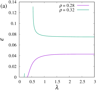
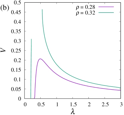
Figure 12: $\lambda$-dependence of (a) $\varepsilon$ and (b) $V$ at $\alpha=0.5$ and $a=3$ for $\rho=0.28$ and $\rho=0.32$.

Here, we consider the control of the parameter $\lambda$ under a fixed value of $a$. Figure 12 shows $\lambda$-dependence of $\varepsilon$ and $V$ at $\alpha=0.5$ and $a=3$ for $\rho=0.28$ and $\rho=0.32$, and explains how the nonconvexity control proposed here works or fails for the perfect reconstruction. We treat the set of macroscopic fixed points as a sequence generated by shifting the value of $\lambda$. Note that the sequence mainly consists of RS-unstable failure solutions. At $\rho=0.28$, the sequences of $\varepsilon$ and $V$ are connected to zero by decreasing $\lambda$, hence one can potentially attain perfect reconstruction by starting from large $\lambda$ and decreasing $\lambda$. However, at $\rho=0.32$, $\varepsilon$ and $V$ tend to diverge when $\lambda\in(0.2117,0.5530)$ as shown in Figure 12. In this region, the finite RS-unstable fixed points are disappeared, and the SE flow goes to the diverging state, although the state is not allowed as a solution. Figure 13 is an example of SE flow going towards the diverging state in the absence of the solution with finite $\varepsilon$ and $V$, which is observed at $\alpha=0.5,\rho=0.32,\lambda=0.4$ and $a=3$. The discontinuity in the sequence of the macroscopic parameters and the SE flow to the diverging state obstructs the nonconvexity control.

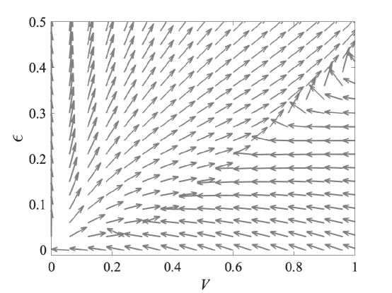
Figure 13: SE flow at $\alpha=0.5$, $\rho=0.32$, $\lambda=0.4$ and $a=3$. There is no fixed point and the flow diverges.

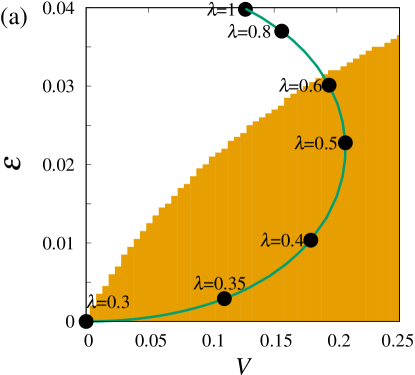
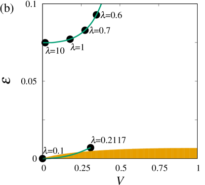
Figure 14: Sequence of macroscopic fixed points of SCAD corresponding to continuous decrease in $\lambda$ at $a=3$ (solid line) and the BOA (shaded region) for a sufficiently small $\lambda$ at $\alpha=0.5$. Dotts denote representative fixed points at the $\lambda$ assigned next to the dotts. (a) Macroscopic fixed points and the BOA at $\lambda=0.3$ is shown for $\rho=0.28$. (b) Macroscopic fixed points and the BOA at $\lambda=0.1$ is shown for $\rho=0.32$.

In Figure 14, we compare the sequence of the macroscopic fixed point with the BOA to the origin at $\alpha=0.5$ and $a=3$ for (a) $\rho=0.28$ and (b) $\rho=0.32$. The solid lines of Figure 14 are drawn by continuously shifting $\lambda$, and are equivalent to Figure 12. Dots on the lines represent examples of the fixed points at each $\lambda$. In Figure 14 (a), the shaded region denotes the BOA to $V=\varepsilon=0$ at $\lambda=0.3$ and $a=3$, where the perfect reconstruction is theoretically supported. To attain perfect reconstruction at this parameter region, we need to prepare the initial condition with $\varepsilon\sim O(10^{-2})$, which is not realistic. However, by decreasing the nonconvexity parameter $\lambda$ from larger values such as $\lambda=1$, the fixed point, which corresponds to RS-unstable failure solution, comes into the BOA to the perfect reconstruction at $\lambda=0.3$ as shown in Figure 14 (a). In Figure 14 (b), BOA to the perfect reconstruction at $\lambda=0.1$ and $a=3$ is depicted as the shaded region at $\alpha=0.5$ and $\rho=0.32$. For larger $\rho$, the sequence of the fixed point shows discontinuity as shown in Figure 14(b), which is caused by the diverging property of the macroscopic quantities as shown in Figs. 12 and 13. It is expected that the sequence of the fixed point below $\lambda=0.2117$ can provide a clue to attain the perfect reconstruction, but corresponding BOA is already shrunk.

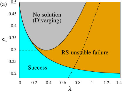
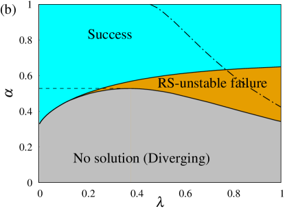
Figure 15: Phase diagram on (a) $\rho-\lambda$ plane at $\alpha=0.5$ and $a=3$ and (b) $\alpha-\lambda$ plane at $\rho=0.32$ and $a=3$. The horizontal dashed lines denote the nonconvexity control limit (a) $\rho_{\mathrm{NCC}}(\alpha=0.5)$ and (b) $\alpha_{\mathrm{NCC}}(\rho=0.32)$. On the left of the dotted-dashed line, the diverging state is stable and the SE flow tends to diverge.

Based on the abovementioned observations, we define nonconvexity control limit (NCC limit) $\rho_{\mathrm{NCC}}(\alpha)$ as the largest value of $\rho$ under given $\alpha$ at which the sequence of the fixed points reach $V=\varepsilon=0$ as $\lambda$ decreases without facing to the discontinuity due to the divergence of the macroscopic parameters; $\alpha_{\rm NCC}(\rho)$ is defined as well. Figure 15(a) and (b) show the phase diagram on $\rho-\lambda$ plane at $\alpha=0.5$ and $a=3$, and that on $\alpha-\lambda$ plane at $\rho=0.32$ and $a=3$. The NCC limit is denoted by the horizontal dashed lines, and the stability of the diverging state (77) is satisfied on the left side of dotted-dashed lines. At $\rho<\rho_{\mathrm{NCC}}$ or $\alpha>\alpha_{\mathrm{NCC}}(\rho)$, the sequence of the fixed point is connected to $V=\varepsilon=0$ by decreasing $\lambda$ as shown in Figure 14 (a). Examples of the SE’s flow below the NCC limit in the RS-unstable failure and the success region are shown in Figure 10 (a) and (b), respectively. At $\rho>\rho_{\mathrm{NCC}}$ or $\alpha<\alpha_{\mathrm{NCC}}$, “No solution” region, in which SE does not have any fixed points in $\Omega^{\dagger}(a)$ and diverges, appears between “Success” region and “RS-unstable failure” region, and the nonconvexity control fails due to the “No solution” region. An example of the SE flow in the “No solution” region is Figure 13. As $\lambda$ increases, the RS-unstable failure phase and the success phase are connected to each other for any $\rho$. This property is the same as the $\ell_{1}$ minimization.

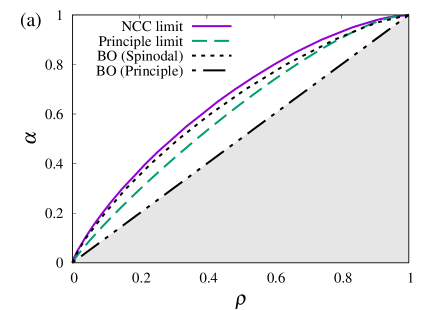
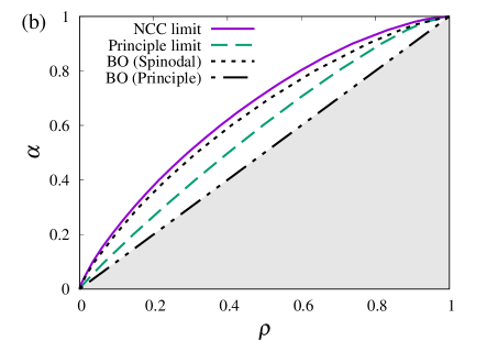
Figure 16: Reconstruction limit by nonconvexity control (NCC limit) and the phase transition boundary (Principle limit) at $\lambda=0.1$ and $a=3$ for (a) SCAD and (b) MCP. For comparison, the algorithmic limit of Bayes optimal method (BO, Spinodal) and the principle limit of Bayes optimal method (BO, Principle) are shown.

Figure 16 shows the $\alpha$-dependence of the NCC limit $\rho_{\mathrm{NCC}}(\alpha)$ for (a) SCAD and (b) MCP. The dependency of $\rho_{\mathrm{NCC}}$ on $a$ is weak; the changes in $a$ induce the changes in the $\rho$ value smaller than $O(10^{-3})$, and here the value is maximized with respect to $a$. For comparison, the phase transition boundary $\alpha_{c}(\rho)$ for $\lambda=0.1$ and $a=3$ is shown as principle limit in the sense that the stability of the success solution is guaranteed. According to the principle limit, it is expected that MCP can achieve perfect reconstruction under denser signals than SCAD, but its NCC limit inferior to SCAD in the order $O(10^{-2})$ in terms of $\rho$. This observation implies that there remains a room for improvement in designing nonconvex penalties to overcome the basin shrinkage sustaining global stability of $V=\varepsilon=0$ in dense region.

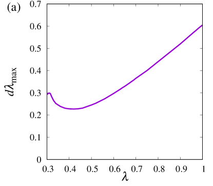
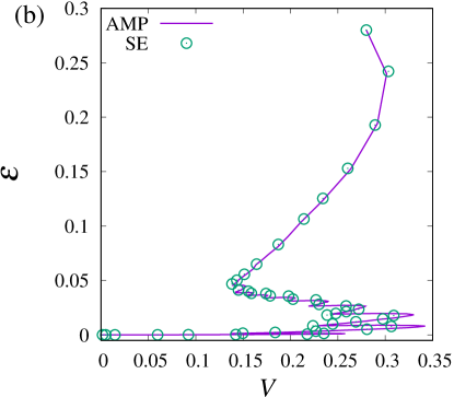
Figure 17: (a) The value of $d\lambda_{\max}$ below which the nonconvexity control is effective at $\alpha=0.5$, $\rho=0.28$ and $a=3$. (b) Trajectory on $V-\varepsilon$ plane with convexity control of SCAD. The trajectories of AMP for one realization of $\bm{X}^{0}$ and $A$ at $N=10^{5}$ (solid line) and SE (circles) are shown. The initial condition is set to be $V=E=\rho$, and $\lambda=1$, $a=3$. The value of $\lambda$ is decreased by $d\lambda=0.1$ after the convergence of $\hat{V}^{(t)}$ and $D^{(t)}$ at each $\lambda$.

The problem in practice is the protocol of the nonconvexity control. We consider here an ‘equilibrium’ approach; we spend sufficient time steps at each $\lambda$ for the convergence to the macroscopic fixed point, which corresponds to the RS-unstable failure solution, and after that we decrease $\lambda$ by $d\lambda$. Hence, we need to set the sufficient time for ‘equilibration’ and $d\lambda$ appropriately. However, we cannot assess $\hat{\varepsilon}^{(t)}$ in AMP’s trajectory since its calculation requires the unknown true signal $\bm{x}^{0}$. Instead, we observe $\hat{V}^{(t)}$ and $\hat{D}^{(t)}\equiv\frac{1}{N}\sum_{i=1}^{N}(\hat{x}_{i}^{(t+1)}-\hat{x}_{i}^{(t)})^{2}$ as criteria of the convergence, and we decrease $\lambda$ by $d\lambda$ after the saturation of the $\hat{V}^{(t)}$ and $\hat{D}^{(t)}$ around certain values. Next, in determining $d\lambda$, the macroscopic fixed point at $\lambda$ is required to be in the BOA of the macroscopic fixed point at $\lambda-d\lambda$ for the effective nonconvexity control. We denote the maximum value of $d\lambda$ as $d\lambda_{\max}$ over which the abovementioned condition is violated, and choose a value $d\lambda$ smaller than $d\lambda_{\max}$ for nonconvexity control. The value of $d\lambda_{\max}$ assessed by SE at $\alpha=0.5$ and $\rho=0.28$ is shown as the solid line in Figure 17(a), where $d\lambda_{\max}$ is obtained by observing the SE flow at $\lambda-d\lambda$ starting from the fixed point at $\lambda$ for various $d\lambda$. Here, we note that at this parameter region, the perfect reconstruction is possible at $\lambda<0.3$, hence $d\lambda$ for $\lambda<0.3$ is trivially $d\lambda\sim\lambda$.

The value of $d\lambda$ shown in Figure 17(a) is for the typical realization of $A$ and $\bm{x}^{0}$, and the possible value of $d\lambda$ might fluctuate depending on $A$ and $\bm{x}^{0}$. To be on the safe side, we set $d\lambda=0.1$ for any $\lambda$ in applying the nonconvexity control to AMP under a given $A$ and $\bm{x}^{0}$. Figure 17(b) shows the actual trajectory of AMP (solid line) for one realization of $A$ and $\bm{x}^{0}$ at $N=10^{5}$, and corresponding SE (circles) at $\alpha=0.5$, $\rho=0.28$ under nonconvexity control. The initial condition of AMP is set to be $\bm{x}=\bm{0}$ and $\bm{v}=\rho\bm{1}_{N}$, where $\bm{1}_{N}$ is the $N$-dimensional vector whose all components are 1, and hence that of SE is $V=E=\rho$. We start with $\lambda=1$ at $a=3$, and decrease $\lambda$ by $d\lambda=0.1$ after the convergence of $\hat{V}^{(t)}$ and $\hat{D}^{(t)}$ at each $\lambda$, until $\lambda$ becomes to be 0.3. The behavior of AMP is well described by SE. Comparing to the flow of SE (Figure 10 (b)), the trajectory of AMP with nonconvexity control approaches the BOA connected to the success solution at $\lambda=0.1$ that is almost on the $V$ axis.

6 Summary and discussion

We have analytically derived the perfect reconstruction limit of the sparse signal in compressed sensing by the minimization of nonconvex sparse penalties, SCAD and MCP. In particular, when the nonconvexity parameters are small, SCAD and MCP minimization reconstruct dense signals that are beyond the $\ell_{1}$ reconstruction limit. This analytical result also appears to imply that SCAD and MCP minimization overcomes the algorithmic limit of the Bayes optimal method, but the numerical experiments using AMP have shown that this is actually not the case. The gap between the analytical and numerical results has been understood by observing the flow of SE, revealing the failure of AMP comes from the shrinking BOA and the divergent behavior of AMP in some parameter region. We have found that SCAD and MCP minimization show a novel failure scenario of the algorithm different from the Bayes-optimal setting where the algorithmic limit is characterized by the emergence of local minima. To mitigate the abovementioned gap and determine the algorithmic limit of AMP, we have proposed the protocol of the nonconvexity control, leading to a largely improved performance.

Originally, SCAD and MCP were designed to satisfy the continuity and the oracle property, which is the simultaneous appearance of the asymptotic normality and consistency, at a certain limit with respect to the nonconvexity parameters [11, 12]. However, such property is not sufficient for practical usage. The design of the nonconvex penalties that does not lead to a shrinkage of basin is another possibility for nonconvex compressed sensing. From the relationship between the sparse prior in Bayesian approach and sparse penalty in frequentist approach, it is implied that SCAD and MCP can be related to the Bernoulli-Gaussian prior in Bayesian terminology with large variance [25]. Unified understanding of the sparsity over Bayesian and frequentist approach will be helpful for designing such desirable sparse penalties. Further, the application of the nonconvexity control to the general matrix beyond that consists of i.i.d. entries should be discussed for practical usage. The rotationally invariant matrix is one of the candidates to examine the effectiveness of the nonconvexity control for general matrix [26, 27, 28].

References

References

- [1] Candés E J and Tao T 2006 IEEE transactions on information theory 52 5406–5425
- [2] Donoho D L 2006 IEEE Transactions on information theory 52 1289–1306
- [3] Chen S S, Donoho D L and Saunders M A 2001 SIAM Review 43 129–159
- [4] Tropp J A 2007 IEEE Transaction on Information Theory 53 4655–4666
- [5] Donoho D L, Maleki A and Montanari A 2011 IEEE Transaction on Information Theory 57 6920 – 6941
- [6] Chartrand R and Yin W 2008 Iteratively reweighted algorithms for compressive sensing IEEE International Conference on Acoustics, Speech and Signal Processing (IEEE) pp 3869–3872
- [7] Gribonval R and Nielsen M 2003 IEEE Transaction on Information Theory 49 3320
- [8] Candés E J 2008 Comptes Rendus Mathematique 346 589–592
- [9] Chartrand R 2007 IEEE Signal Process. Lett. 14 707–710
- [10] Chartrand R and Staneva S 2008 Inverse Problems 24 035020
- [11] Fan J and Li R 2001 Journal of the American statistical Association 96 1348–1360
- [12] Zhang C H 2010 The Annals of Statistics 38 894–942
- [13] Sakata A and Xu Y 2018 \JSTAT 2018 033404
- [14] Donoho D L 2006 Discrete & Computational Geometry 35 617–652
- [15] Donoho D L and Tanner J 2009 Journal of American Mathematical Society 22 1–53
- [16] Kabashima Y, Wadayama T and Tanaka T 2009 Journal of Statistical Mechanics: Theory and Experiment 2009 L09003
- [17] Krzakala F, Mézard M, Sausset F, Sun Y and Zdeborová L 2012 Journal of Statistical Mechanics: Theory and Experiment 2012 P08009
- [18] Sakata A 2018 \JSTAT 2018 063404
- [19] Sakata A 2016 \JSTAT 2016 123302
- [20] De Almeida J and Thouless D J 1978 Journal of Physics A: Mathematical and General 11 983
- [21] Rangan S 2011 Generalized approximate message passing for estimation with random linear mixing Information Theory Proceedings (ISIT), 2011 IEEE International Symposium on (IEEE) pp 2168–2172
- [22] Obuchi T, Nakanishi-Ohno Y, Okada M and Kabashima Y 2018 \JSTAT 2018 103401
- [23] Mezard M and Montanari A 2009 Information, physics, and computation (Oxford University Press)
- [24] Bayati M and Montanari A 2011 IEEE Transaction on Information Theory 57 764–785
- [25] G Polson N and Sun L 2018 Applied Stochastic Models in Business and Industry 35 717–731
- [26] Schniter P, Rangan S and Fletcher A K 2017 Vector approximate message passing Information Theory Proceedings (ISIT), 2017 IEEE International Symposium on (IEEE) pp 1588–1592
- [27] Gerbelot C, Abbara A and Krzakala F 2020 Asymptotic errors for high-dimensional convex penalized linear regression beyond gaussian matrices Proceedings of Machine Learning Research, 33rd Annual Conference on Learning Theory (MLR press) pp 1–32
- [28] Takahashi T and Kabashima Y 2020 Macroscopic analysis of vector approximate message passing in a model mismatch setting Information Theory Proceedings (ISIT), 2020 IEEE International Symposium on (IEEE) pp 1403–1408