Impact of form factor uncertainties on interpretations of
coherent elastic neutrino-nucleus scattering data

Abstract

The standard model coherent elastic neutrino-nucleus scattering (CE$\nu$NS) cross section is subject to nuclear form factor uncertainties, mainly driven by the root-mean-square radius of the neutron density distribution. Motivated by COHERENT phases I-III and future multi-ton direct detection dark matter searches, we evaluate these uncertainties in cesium iodide, germanium, xenon and argon detectors. We find that the uncertainties become relevant for momentum transfers $q\gtrsim 20$ MeV and are essentially independent of the form factor parameterization. Consequently, form factor uncertainties are not important for CE$\nu$NS induced by reactor or solar neutrinos. Taking into account these uncertainties, we then evaluate their impact on measurements of CE$\nu$NS at COHERENT, the diffuse supernova background (DSNB) neutrinos and sub-GeV atmospheric neutrinos. We also calculate the relative uncertainties in the number of COHERENT events for different nuclei as a function of recoil energy. For DSNB and atmospheric neutrinos, event rates at a liquid argon detector can be uncertain to more than 5%. Finally, we consider the impact of form factor uncertainties on searches for nonstandard neutrino interactions, sterile neutrinos and neutrino generalized interactions. We point out that studies of new physics using CE$\nu$NS data are affected by neutron form factor uncertainties, which if not properly taken into account may lead to the misidentification of new physics signals. The uncertainties quantified here are also relevant for dark matter direct detection searches.

I Introduction

Coherent elastic neutrino-nucleus scattering (CE$\nu$NS) was observed by the COHERENT experiment in 2017 in a cesium iodide scintillation detector. The measurement used neutrinos produced at the spallation neutron source at the Oak Ridge National Laboratory Akimov et al. (2017). The cross section, obtained by the coherent sum of the individual nucleon amplitudes, is the largest of all neutrino cross sections at energies $E_{\nu}\lesssim 100$ MeV, exceeding the elastic neutrino-electron scattering cross section by about two orders of magnitude in typical nuclei. The observation, however, relies on the detection of very small recoil energies, which only recently became possible with the use of the technology employed in direct detection dark matter (DM) searches.

CE$\nu$NS data allow precise measurements of the weak mixing angle Cañas et al. (2018), detailed studies of nuclear structure through weak neutral current interactions Patton et al. (2012) and opens the possibility of searching for new physics beyond the standard model (SM) Barranco et al. (2005); Scholberg (2006). Indeed, since its observation various studies of nonstandard neutrino interactions (NSI) Coloma et al. (2017); Liao and Marfatia (2017); Papoulias and Kosmas (2018); Billard et al. (2018), sterile neutrinos Billard et al. (2018), neutrino generalized interactions (NGI) Aristizabal Sierra et al. (2018) and neutrino electromagnetic properties Papoulias and Kosmas (2018); Cadeddu et al. (2018a) have been presented. A proper interpretation of a CE$\nu$NS signal, as related to any of these new physics scenarios, requires a detailed understanding not only of experimental systematics errors but also of theoretical uncertainties.

The calculation of event rates in CE$\nu$NS experiments involves proton and neutron nuclear form factors, which account for the proton and neutron distributions within the nucleus. In most treatments, however, the form factors are assumed to be equal and so the nuclear form factor becomes a global factor, which is typically parameterized in terms of the Helm Helm (1956) form factor, the Fourier transform of the symmeterized Fermi distribution Sprung and Martorell (1997), or the Klein-Nystrand form factor Klein and Nystrand (1999) as adopted by the COHERENT collaboration  Akimov et al. (2017). These form factors depend on various parameters whose values are fixed via experimental data and so involve experimental uncertainties. Of particular relevance is the root-mean-square (rms) radius of the nucleon distribution, which in such analyses is fixed by, for example, the value derived using a particular nuclear physics model or through a value derived from fits to nuclear data Lewin and Smith (1996). This simplification introduces an uncertainty on the predicted CE$\nu$NS recoil spectrum (and number of events) in the SM as well as in beyond-the-standard-model (BSM) physics scenarios.

The root-mean-square (rms) radius of the proton distribution $r_{\text{rms}}^{p}$ is known from elastic electron-nucleus scattering with a precision of order one-per-mille for nuclear isotopes up to $Z=96$ Angeli and Marinova (2013). This is in sharp contrast with the rms radius of the neutron distribution $r_{\text{rms}}^{n}$, which for almost all nuclear isotopes is poorly known. Theoretical uncertainties on the CE$\nu$NS process are therefore driven by the uncertainties in $r_{\text{rms}}^{n}$. For the COHERENT experiment, the quenching factor and neutrino flux uncertainties are of order 27% Akimov et al. (2017, 2018a). Thus, form factor uncertainties are not particularly relevant in the interpretation of current data. This situation, however, is expected to change in the near future, and so form factor uncertainties will play an important role.

Identifying the size of these uncertainties is crucial for two reasons: (i) To understand whether a given signal is the result of new physics or of an “unexpected” nuclear physics effect, (ii) DM direct detection in hundred-ton scale detectors like Argo Aalseth et al. (2018), will be subject to irreducible neutrino backgrounds from the diffuse supernova background (DSNB) and sub-GeV atmospheric neutrino fluxes. A precise understanding of this background is crucial to discriminate between neutrino-induced and WIMP-induced signals.

With this in mind, in this paper we investigate the size and behavior of the neutron nuclear form factor uncertainties and their impact on the interpretation of data. To that end we consider four well-motivated nuclei: cesium iodide, germanium, xenon and argon. The first three are (or will be) used by COHERENT in one of its three phases Akimov et al. (2015), while argon will be used by the Argo detector of the Global Argon Dark Matter Collaboration which will take 1000 ton-year of data Aalseth et al. (2018). For definitiveness we consider three nuclear form factor parameterizations: The Helm form factor Helm (1956), the Fourier transform of the symmeterized Fermi distribution Sprung and Martorell (1997) and the Klein-Nystrand form factor Klein and Nystrand (1999). And we assume the same parameterization for both protons and neutrons. We first study the size and momentum transfer ($q$) dependence of the neutron form factor uncertainties using these three parameterizations. After precisely quantifying them, we study their impact in COHERENT and in an argon-based multi-ton DM detector. We assess as well the impact of the uncertainties on the interpretation of new physics effects. We do this in the case of NSI, active-sterile neutrino oscillations in the 3+1 framework and spin-independent NGI. We evaluate the effects of the neutron form factor uncertainties on the available parameter space and the potential misidentification of new physics signals when these uncertainties are not properly accounted for.

The paper is organized as follows. In Section II we introduce our notation and briefly discuss the CE$\nu$NS process, focusing on form factor parameterizations and the corresponding rms radii of the nucleon density distributions. In Section III we quantify the size of the neutron form factor uncertainties, study their $q$ dependence and show that they are fairly independent of the choice of the nuclear form factor. In Sections IV and V we study the implications for SM predictions and for new physics searches, respectively. In Section VI we present our conclusions. In Appendix A we present the details of the calculation of the DSNB neutrino flux, while in Appendix B we provide details of the NGI analysis.

II Coherent elastic neutrino-nucleus scattering

For neutrino energies below $\sim 100$ MeV the de Broglie wavelength of the neutrino-nucleus process is larger than the typical nuclear radius and so the individual nucleon amplitudes add coherently. In the SM this translates into a cross section that is approximately enhanced by the number of constituent neutrons $N$ Freedman (1974); Freedman et al. (1977):

$$\frac{d\sigma}{dE_{r}}=\frac{G_{F}^{2}m_{N}}{2\pi}\left(2-\frac{E_{r}m_{N}}{E_{\nu}^{2}}\right)\left[Ng_{V}^{n}F_{N}(q^{2})+Zg_{V}^{p}F_{Z}(q^{2})\right]^{2}\,,$$ (1)

where $E_{r}=q^{2}/2m_{N}$ is the nuclear recoil energy. This result follows from the vector neutral current. The axial current contribution, being spin dependent, is much smaller. The neutron and proton charges are given by $g_{V}^{n}=-1/2$ and $g_{V}^{p}=1/2-2\sin^{2}\theta_{W}$, with $\theta_{W}$ the weak mixing angle. In the Born approximation, the nuclear form factors $F_{N,Z}(q^{2})$ follow from the Fourier transform of the neutron and proton density distributions. They capture the behavior one expects: the cross section should fall with increasing neutrino energy (increasing $q$). Theoretical predictions based on Eq. (1) involve uncertainties from electroweak parameters and nuclear form factors. These uncertainties should be accounted for and are particularly important in searches for new physics effects, which arguably are not expected to significantly exceed the SM expectation. Since the uncertainty in $G_{F}$ is a few tenths of a part per million Tishchenko et al. (2013), electroweak uncertainties are dominated by the weak mixing angle for which (using the $\overline{\text{MS}}$ renormalization scheme at the $Z$ boson mass scale) the PDG gives Tanabashi et al. (2018)

$$\sin^{2}\theta_{W}=0.23122\pm 0.00003\,.$$ (2)

Electroweak uncertainties are therefore of no relevance. On the contrary, since nuclear form factors encode information on the proton and neutron distributions one expects these uncertainties to be sizable and more pronounced for large $q$, given the behavior $F(q^{2}\to 0)\to 1$. These uncertainties turn out to be crucial for the interpretation of data from fixed target experiments such as COHERENT Akimov et al. (2017, 2018a) and for DM direct detection experiments subject to diffuse supernova background (DSNB) and sub-GeV atmospheric neutrinos Billard et al. (2014).

II.1 Nuclear form factors

Form factors are introduced to account for the density distributions of nucleons inside the nucleus. They follow from the Fourier transform of the nucleon distributions,

$$F(q^{2})=\int\,e^{i\vec{q}\cdot\vec{r}}\,\rho(r)\,d^{3}\vec{r}\ .$$ (3)

The basic properties of nucleonic distributions are captured by different parameterizations. Here we consider those provided by the Helm model Helm (1956), the symmeterized Fermi distribution Sprung and Martorell (1997) and the Klein-Nystrand approach Klein and Nystrand (1999). These distributions depend on two parameters which measure different nuclear properties and which are constrained by means of the rms radius of the distribution,

$$r_{\text{rms}}^{2}\equiv\langle r^{2}\rangle=\frac{\int\,\rho(r)\,r^{2}\,d^{3}\vec{r}}{\int\,\rho(r)\,d^{3}\vec{r}}\ .$$ (4)

In what follows we briefly discuss these parameterizations and the relations between their defining parameters and the rms radius of the distributions. These relations are key to our analysis for they determine, through the experimental uncertainties in $r_{\text{rms}}$, the extent up to which these parameters can vary, thereby defining the form factor uncertainties.

In the Helm model the nucleonic distribution is given by a convolution of a uniform density with radius $R_{0}$ (box or diffraction radius) and a Gaussian profile. The latter is characterized by the folding width $s$, which accounts for the surface thickness. Thus, the Helm distribution reads

$$\rho_{H}(r)={3\over 4\pi R_{0}^{3}}\,\int\,f_{G}(r-r^{\prime})\theta(R_{0}-|r^{\prime}|)d^{3}\vec{r^{\prime}}\ ,$$ (5)

with $\theta(x)$ a Heaviside step function and $f_{G}(x)$ a Gaussian distribution given by

$$f_{G}(x)=\frac{e^{-x^{2}/2s^{2}}}{\sqrt{(2\pi)^{3}}s^{3}}\,.$$ (6)

The Helm form factor is then derived from Eqs. (3) and (5):

$$F_{\text{H}}(q^{2})=3\frac{j_{1}(qR_{0})}{qR_{0}}e^{-q^{2}s^{2}/2}\,,$$ (7)

where $j_{1}(x)=\sin(x)/x^{2}-\cos(x)/x$ is a spherical Bessel function of order one. The rms radius is obtained from Eqs. (4) and (5) and is given by

$$\langle r^{2}\rangle_{\text{H}}=\frac{3}{5}R_{0}^{2}+3s^{2}\,.$$ (8)

The symmeterized Fermi density distribution $\rho_{\text{SF}}(r)$ follows from the symmeterized Fermi function $f_{\text{SF}}(r)=f_{\text{F}}(r)+f_{\text{F}}(-r)-1$, which in turn follows from the conventional Fermi, or Woods-Saxon function,

$$f_{\text{F}}(r)=\frac{1}{1+e^{(r-c)/a}}\ ,$$ (9)

where $c$ is the half-density radius and $a$ represents the surface diffuseness. Accordingly, $\rho_{\text{SF}}(r)$ can be written as

$$\rho_{\text{SF}}(r) =\frac{3}{4\pi c(c^{2}+\pi^{2}a^{2})}\frac{\sinh(c/a)}{\cosh(r/a)+\cosh(c/a)}\,.$$ (10)

In contrast to the Fermi density distribution it has the advantage that its Fourier transform can be analytically evaluated with the result,

$$F_{\text{SF}}(q^{2}) =\frac{3}{qc}\left[\frac{\sin(qc)}{(qc)^{2}}\left(\frac{\pi qa}{\tanh(\pi qa)}\right)-\frac{\cos(qc)}{qc}\right]$$

$$\times\left(\frac{\pi qa}{\sinh(\pi qa)}\right)\frac{1}{1+(\pi a/c)^{2}}\ .$$ (11)

Then,

$$\langle r^{2}\rangle_{\text{SF}}=\frac{3}{5}c^{2}+\frac{7}{5}(\pi a)^{2}\ .$$ (12)

The Klein-Nystrand approach relies on a surface-diffuse distribution which results from folding a short-range Yukawa potential with range $a_{k}$, over a hard sphere distribution with radius $R_{A}$. The Yukawa potential and the hard sphere distribution can be written as

$$V_{\text{Y}}(r)=\frac{e^{-r/a_{k}}}{4\pi a_{k}^{2}r}\ ,\qquad\rho_{\text{HS}}(r)=\frac{3}{4\pi R_{A}^{3}}\theta(R_{A}-r)\ .$$ (13)

The Klein-Nystrand form factor can then be calculated as the product of two individual Fourier transformations, one of the potential and another of the hard sphere distribution, resulting in

$$F_{\text{KN}}(q^{2})=F_{\text{Y}}(q^{2})F_{\text{HS}}(q^{2})=3\frac{j_{1}(qR_{A})}{qR_{A}}\frac{1}{1+q^{2}a_{k}^{2}}\ .$$ (14)

The rms radius is given by

$$\langle r^{2}\rangle_{\text{KN}}=\frac{3}{5}R_{A}^{2}+6a_{k}^{2}\ .$$ (15)

III Form factor uncertainties

The rms radii of the proton density distributions are determined from different experimental sources. The values reported in Angeli and Marinova (2013) include data from optical and $K_{\alpha}$ X-ray isotope shifts as well as muonic spectra and electronic scattering experiments. This wealth of data has allowed the determination of $\sqrt{\langle r^{2}_{p}\rangle}\equiv r_{\text{rms}}^{p}$ with high accuracy for all isotopes of interest for CE$\nu$NS and DM direct detection experiments. The rms radii for the proton distribution are as in Table 1. In contrast, rms radii of the neutron density distributions $\sqrt{\langle r^{2}_{n}\rangle}\equiv r_{\text{rms}}^{n}$ are poorly known, mainly because barring the cases of ²⁰⁸Pb, ¹³³Cs and ¹²⁷I Abrahamyan et al. (2012); Horowitz et al. (2012, 2014); Cadeddu et al. (2018b), their experimental values follow from hadronic experiments which are subject to large uncertainties.

			Argon			Germanium						Xenon
	127I	$4.750$	36Ar	($0.33\%$)	$3.390$	70Ge	($20.4\%$)	$4.041$	72Ge	($27.3\%$)	$4.057$	124Xe	($0.095\%$)	$4.766$	126Xe	($0.089\%$)	$4.774$	128Xe	($1.91\%$)	$4.777$
	133Cs	$4.804$	38Ar	($0.06\%$)	$3.402$	73Ge	($7.76\%$)	$4.063$	74Ge	($36.7\%$)	$4.074$	129Xe	($26.4\%$)	$4.777$	130Xe	($4.07\%$)	$4.781$	131Xe	($21.2\%$)	$4.780$
	—	—	40Ar	($99.6\%$)	$3.427$	76Ge	($7.83\%$)	$4.09$	—	—	—	132Xe	($26.9\%$)	$4.785$	134Xe	($10.4\%$)	$4.789$	136Xe	($8.86\%$)	$4.796$

Table 1: Rms radii (in fm) of the proton density distributions of the stable isotopes of cesium, iodine, argon, germanium and xenon Angeli and Marinova (2013). The relative abundances of the Ar, Ge and Xe isotopes are provided in parentheses.

At the form factor level, therefore, uncertainties on $r_{\text{rms}}^{p}$ are basically irrelevant while uncertainties in $r_{\text{rms}}^{n}$ have a substantial effect. Consequently, we adopt the following procedure. We verified that adopting different form factor parameterizations for the proton and neutron distributions leads to a small effect on our results, so we assume the same form factor for both. For protons, in each of Eqs. (8), (12) and (15), we fix one parameter and determine the other by fixing $r_{\text{rms}}^{p}$ to its experimental central value. For neutrons we do the same as that for protons, but restrict $r_{\text{rms}}^{n}$ to values above $r_{\text{rms}}^{p}$; this lower limit is reliable provided $N>Z$, which is the case for all nuclei we consider. For nuclei other than argon, we fix the upper limit using the neutron skin, $\Delta r_{np}=r_{\text{rms}}^{n}-r_{\text{rms}}^{p}$, of ²⁰⁸Pb, which is measured by the PREX experiment at Jefferson laboratory to be $\Delta r_{np}(^{208}\text{Pb})=0.33^{+0.16}_{-0.18}$ fm Horowitz et al. (2012, 2014); while PREX-II and CREX will measure the neutron skins of ${}^{208}\text{Pb}$ and ${}^{48}\text{Ca}$, respectively Horowitz et al. (2014), no measurements of the neutron skin of the nuclei we are considering are planned. Experiments have focused on the doubly-magic nuclei, ²⁰⁸Pb and ⁴⁸Ca, because for such nuclei theoretical calculations are under relatively good control. Pairing correlations and deformation become relevant for nuclei that are not doubly-magic. The situation is worse for nuclei with unpaired nucleons like ¹³³Cs, ¹²⁷I and ¹²⁹Xe, in which case calculations assume that the nuclei are even-even nuclei (although they are not), and rescale the occupancy of the valence orbital by a suitable factor with the hope that bulk properties like the weak radius are not sensitive to this “spherical approximation” Piekarewicz .

We then require the neutron skin of the heavy nuclei to be no larger than 0.3 fm given that their values of $(N-Z)/(N+Z)$ are less than for ${}^{208}\text{Pb}$. We use

$$r_{\rm{rms}}^{n}|_{\rm max}\equiv r_{\rm{rms}}^{p}+0.3~{}{\rm fm}\ \ \ \text{for Cs, I, Ge and Xe.}$$ (16)

For argon, we allow the neutron skin to lie between 0.1 fm and 0.2 fm, i.e.,

$$r_{\rm{rms}}^{n}|_{\rm max}\equiv r_{\rm{rms}}^{p}+0.1~{}\text{fm\ \ \ or\ \ \ }~{}r_{\rm{rms}}^{p}+0.2~{}{\rm fm}\ \ \ \text{for Ar.}$$ (17)

Note that these large values of $\Delta r_{np}$ parameterize the envelope of the form factors from different calculation methods including chiral effective field theory, relativistic and nonrelativistic mean-field models, etc. It is a proxy for the spread in theoretical predictions of the form factor, and is not intended as an estimate of its value.

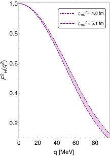
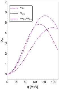
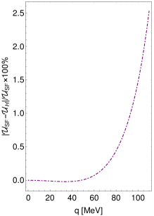
Figure 1: Left: Square of the Helm form factor as a function of the momentum transfer $q$. The upper (lower) curve is obtained by fixing $\sqrt{\langle r^{2}\rangle_{\text{H}}}$ to $r_{\text{rms}}^{p}$ ($r_{\text{rms}}^{p}+0.3$ fm) as given in Table 1 for ¹³³Cs. Middle: Percentage uncertainty for ¹³³Cs, ¹²⁹Xe, ⁷⁴Ge and ⁴⁰Ar (for ⁴⁰Ar, we take $r_{\rm{rms}}^{n}|_{\rm max}=r_{\text{rms}}^{p}+0.2$ fm). It can be seen that uncertainties get larger as $q$ increases to 65 MeV. Right: Relative difference between the Helm and symmeterized Fermi form factors uncertainties for ${}^{133}\text{Cs}$. Using the Klein-Nystrand form factor yields results of the same order and so are not displayed. The main point is that the size of the uncertainties do not depend on the form factor chosen.

For the Helm form factor we fix the surface thickness $s$ to 0.9 fm Lewin and Smith (1996), for the form factor based on the symmeterized Fermi function we fix the surface diffuseness $a$ to 0.52 fm Piekarewicz et al. (2016) and for the Klein-Nystrand form factor we fix the range $a_{k}$ of the Yukawa potential to 0.7 fm Klein and Nystrand (1999). We checked that our results are rather insensitive to variations of these values. With the procedure already outlined, we first investigate the behavior of the uncertainties and their size. Figure 1 shows the result for the Helm form factor obtained for ¹³³Cs. The left panel shows that for low $q$, the uncertainties are small and increase with increasing momentum, reaching their maximum for $q\simeq 65$ MeV. This behavior is apparent in the middle panel which shows the Helm percentage uncertainty,

$$\mathcal{U}_{H}=\left|F_{H}^{2}(q^{2})|_{r_{\text{rms}}^{n}=r_{\text{rms}}^{p}}-F_{H}^{2}(q^{2})|_{r_{\text{rms}}^{n}=r_{\text{rms}}^{p}+0.3\,\text{fm}}\right|\times 100\%\ ,$$ (18)

which measures the size of the spread due to the uncertainties in $r_{\text{rms}}^{n}$; for argon, 0.3 fm is replaced by 0.2 fm in the above equation. It can be seen that in the case of ¹³³Cs the uncertainty can be as large as 5%, and for ⁴⁰Ar as large as $4.5\%$. To address how this result depends on the choice of form factor, we calculate the percentage uncertainty for $F_{\text{SF}}$ and $F_{\text{KN}}$, with the aid of Eqs. (12) and (15). The right panel in Fig. 1 shows the relative uncertainty obtained by comparing the uncertainties from the Helm and the symmeterized Fermi form factors, calculated according to $|\mathcal{U}_{\text{SF}}-\mathcal{U}_{\text{H}}|/\mathcal{U}_{\text{SF}}\times 100\%$; results using the Klein-Nystrand form factor are similar and are not displayed. It can be seen that uncertainties are parameterization independent for $q$ up to 60 MeV or so. For larger $q$, differences are at most of order $2.5\%$, with the Helm form factor yielding slightly larger values. In summary, the conclusions derived from Fig. 1 hold no matter the form factor choice. Henceforth, to calculate the impact of the form factor uncertainties on CE$\nu$NS, we employ the Helm form factor.

IV Implications for COHERENT, DSNB and sub-GeV atmospheric neutrinos

We now turn to the study of the impact of the form factor uncertainties on SM predictions for CE$\nu$NS. We begin with COHERENT in each of its phases. For phase-I we calculate the expected number of events taking into account the contributions from both ¹³³Cs and ¹²⁷I. For phase-II (germanium phase) and phase-III (LXe phase) we calculate the number of events assuming the specifications given in Akimov et al. (2015) with the number of protons on target ($n_{\text{POT}}$) per year as in the CsI case; event numbers for a different value $n_{\text{POT}}^{\prime}$ can be straightforwardly rederived by scaling our result by $n_{\text{POT}}^{\prime}/n_{\text{POT}}$. Since germanium and xenon have several sufficiently abundant isotopes (see Table 1), we calculate the recoil spectrum generated by each of the nuclides. The $i^{\rm{th}}$ isotope recoil spectrum can be written as

$$\frac{dR_{i}}{dE_{r}}=\frac{m_{\text{det}}N_{A}}{\langle m\rangle}X_{i}\int_{E_{\nu}^{\text{min}}}^{E_{\nu}^{\text{max}}}\,\phi(E_{\nu})\,\frac{d\sigma_{i}}{dE_{r}}\,dE_{\nu}\ ,$$ (19)

where $m_{\text{det}}$ refers to the detector mass, $X_{i}$ to its relative abundance, $\langle m\rangle$ to the average molar mass calculated as $\sum_{k}m_{k}X_{k}$ ($m_{k}$ being the molar mass of the individual isotopes), $N_{A}=6.022\times 10^{23}\,\text{mol}^{-1}$ and $\phi(E_{\nu})$ the neutrino flux. Note that the global factor $(m_{\text{det}}N_{A}/\langle m\rangle)X_{i}$ corresponds to the number of nuclei of the $i^{\rm{th}}$ type in the detector. The differential cross section is given by Eq. (1) with $m_{N}\to m_{i}$, $N\to N_{i}$ and $q^{2}\to q^{2}_{i}=2m_{i}E_{r}$. For each isotope contribution $r_{\text{rms}}^{p}$ is fixed according to the values in Table 1 and $r_{\text{rms}}^{n}$ as described in the previous section. Calculating the individual recoil spectra according to Eq. (19) and then summing over all of them (to determine the total recoil spectrum), allows to properly trace the uncertainties induced by each neutron form factor.

For the COHERENT phase-I analysis we use $m_{\text{det}}=14.6$ kg and adapt Eq. (19) to take into account the contributions of ¹³³Cs and ¹²⁷I. This is done by trading $X_{i}$ for the nuclear fractions $f_{i}=A_{i}/(A_{\text{Cs}}+A_{\text{I}})$ ($A_{i}$ refer to the ¹³³Cs and ¹²⁷I mass numbers) in (19) and $\langle m\rangle$ for $m_{\text{CsI}}=259\times 10^{-3}\,$kg/mol (CsI molar mass). The acceptance function is Akimov et al. (2018a)

$$\mathcal{A}(n_{\text{PE}})=\frac{k_{1}}{1+e^{-k_{2}(n_{\text{PE}}-x_{0})}}\theta(n_{\text{PE}}-5)\ ,$$ (20)

where $k_{1}=0.6655$, $k_{2}=0.4942$, $x_{0}=10.8507$, and $n_{\text{PE}}$ is the observed number of photoelectrons. Neutrino fluxes in COHERENT are produced by $\pi^{+}$ and $\mu^{+}$ decays, and so three neutrino flavors are produced ($\nu_{\mu}$, $\bar{\nu}_{\mu}$ and $\nu_{e}$) with known energy spectra:

$$\mathcal{F}_{\nu_{\mu}}(E_{\nu_{\mu}}) =\frac{2m_{\pi}}{m_{\pi}^{2}-m_{\mu}^{2}}\,\delta\left(1-\frac{2E_{\nu_{\mu}}m_{\pi}}{m_{\pi}^{2}-m_{\mu}^{2}}\right)\ ,$$

$$\mathcal{F}_{\nu_{e}}(E_{\nu_{e}}) =\frac{192}{m_{\mu}}\left(\frac{E_{\nu_{e}}}{m_{\mu}}\right)^{2}\left(\frac{1}{2}-\frac{E_{\nu_{e}}}{m_{\mu}}\right)\ ,$$

$$\mathcal{F}_{\bar{\nu}_{\mu}}(E_{\bar{\nu}_{\mu}}) =\frac{64}{m_{\mu}}\left(\frac{E_{\bar{\nu}_{\mu}}}{m_{\mu}}\right)^{2}\left(\frac{3}{4}-\frac{E_{\bar{\nu}_{\mu}}}{m_{\mu}}\right)\,,$$ (21)

where the neutrino energies are less than $m_{\mu}/2$.

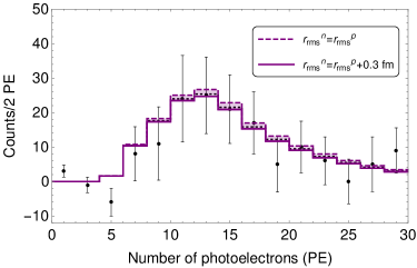
Figure 2: The expected CE$\nu$NS residual event spectrum in COHERENT as a function of the number of photoelectrons as predicted in the SM. The points correspond to COHERENT data (with their error bars) Akimov et al. (2017), while the shaded region between the two histograms defines the uncertainty in the spectrum due to the form factor uncertainties. The black-dotted histogram is obtained by fixing the rms radii of the ¹³³Cs and ¹²⁷I neutron density distributions to values obtained from theoretical calculations; see Eq. (22). For the dashed histogram, $r_{\text{rms}}^{n}=r_{\text{rms}}^{p}$, with the values of $r_{\text{rms}}^{p}$ from Table 1. The Helm form factor has been used but a different form factor does not noticeably alter the spectra.

The neutrino flux per flavor $\phi_{a}(E_{\nu})$ at the detector is obtained by weighting the energy spectra by the normalization factor $\mathcal{N}=r\times n_{\text{POT}}/4\pi L^{2}$. Here $r=0.08$ determines the number of neutrinos produced per proton collision (per flavor), $L=19.3$ m is the distance from the source to the detector, and $n_{\text{POT}}=1.76\times 10^{23}$ is the number of protons on target in the 308.1 days of neutrino production Akimov et al. (2017), which corresponds to $2.1\times 10^{23}\,\text{protons}/\text{year}$. In terms of $n_{\text{PE}}$ we calculate the SM expectation for the number of events per bin (2 photoelectrons) taking into account the neutron form factor uncertainties. The result is displayed in Fig. 2. Uncertainties in the neutron form factor produce an uncertainty in the expected number of events, with a behavior such that small values of $r_{\text{rms}}^{n}$ tend to increase the number of events, while large values tend to decrease them. This is in agreement with the result in the left panel in Fig. 1. One can see as well that for low $n_{\text{PE}}$ (recoil energy), no sizable uncertainties are observed. However, for $n_{\text{PE}}=7$ ($E_{r}=5.98$ keV) uncertainties are of order 4% and increase to about 9% for $n_{\text{PE}}=15$. We also calculate the number of events by fixing the rms radii of the ¹³³Cs and ¹²⁷I neutron density distributions to

$$r_{\text{rms}}^{n}(^{133}\text{Cs})=5.01\ \text{fm}\,,\qquad r_{\text{rms}}^{n}(^{127}\text{I})=4.94\ \text{fm}\,.$$ (22)

These values follow from theoretical calculations using the relativistic mean field (RMF) NLZ2 nuclear model Cadeddu et al. (2018b). The result obtained can then be regarded as purely theoretical. Comparing the black-dotted histogram in Fig. 2 with those determined by the form factor uncertainties we see that the theoretical expectation is closer to the result for $r_{\text{rms}}^{p}$. We have checked that because of the large experimental uncertainties, using different values of $r_{\text{rms}}^{n}$ has almost no effect on the quality of the fit.

COHERENT phase-II consists of a p-type point-contact high purity germanium detector with $m_{\text{det}}=15$ kg and located at $L=22$ m from the source. COHERENT phase-III, instead, aims at measuring CE$\nu$NS by using a two-phase liquid xenon detector with $m_{\text{det}}=100$ kg and located at $L=29$ m. A one ton LAr detector at $L=29$ m is also under consideration. At low recoil energies the number of CE$\nu$NS events in the Xe detector will exceed those in the Ge detector by about an order of magnitude. However, since Ge isotopes are lighter than Xe isotopes, the Ge detector will be sensitive to CE$\nu$NS events at higher recoil energies and so they are complementary Akimov et al. (2015). Using these target masses, the corresponding locations and assuming $n_{\text{POT}}$/year as in the CsI calculation, we calculate the impact of the uncertainties on the expected number of events in both detectors. As can be seen from Fig. 3 in the germanium case relative uncertainties can be sizable, and for Xe, relative uncertainties are still larger. It is clear that form factor uncertainties should be taken into account in the analysis of COHERENT data.

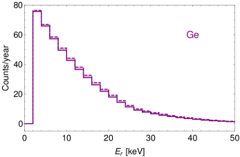
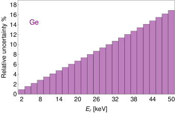
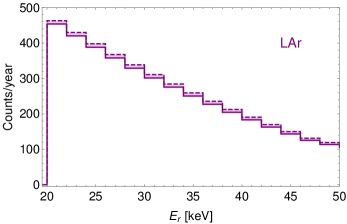
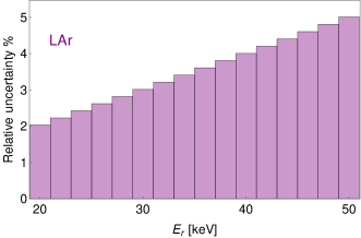
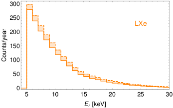
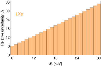
Figure 3: Expected number of CE$\nu$NS events (left) and its relative uncertainty, equal to (maximum count number $-$ minimum count number)$/$(maximum count number)$\times 100$, (right) as a function of recoil energy for argon, germanium and xenon. The calculations have been done for the COHERENT Ge, LAr and LXe detectors including form factor uncertainties, summing the three neutrino flavor contributions and taking $n_{\text{POT}}$ as in the CsI case.

Since form factor uncertainties increase with increasing momentum transfer, they are also relevant for CE$\nu$NS induced by the DSNB and sub-GeV atmospheric neutrinos. DSNB neutrinos (neutrinos and antineutrinos of all flavors) result from the cumulative emission from all past core-collapse supernovae. Their flux is thus determined by the rate for core-collapse supernova (determined in turn by the cosmic star formation history), and the neutrino emission per supernova, properly redshifted over cosmic time Ando and Sato (2004) (see Appendix A for details). The latter is well described by a Fermi-Dirac distribution with zero chemical potential and with $T_{\nu_{e}}<T_{\bar{\nu}_{e}}<T_{\nu_{x}}$ Horiuchi et al. (2009). For the calculation of the DSNB neutrino flux we use $T_{\nu_{e}}=3$ MeV, $T_{\bar{\nu}_{e}}=5$ MeV and $T_{\nu_{x}}=8$ MeV, and sum over all flavors.

Atmospheric neutrino fluxes ($\nu_{e}$ and $\nu_{\mu}$ and their antiparticles) result from hadronic showers induced by cosmic rays in the Earth’s atmosphere. We take the atmospheric fluxes from Ref. Battistoni et al. (2005) generated by a FLUKA Monte Carlo simulation Ferrari et al. (2005), that includes $\nu_{e,\tau}$ and $\bar{\nu}_{e,\tau}$ fluxes up to about $10^{3}$ MeV. We only consider atmospheric neutrino fluxes below 100 MeV because for higher energies the loss of coherence for CE$\nu$NS drastically depletes the neutrino event rate making the flux at those energies less relevant.

Figure 4 shows the event spectrum for the sum of the DSNB and atmospheric neutrino contributions in an argon detector with an exposure of $1000$ ton-year. The dashed (solid) histogram is obtained by fixing $r_{\text{rms}}^{n}=r_{\text{rms}}^{p}$ ($r_{\text{rms}}^{n}=r_{\text{rms}}^{p}+0.2$ fm). In the calculation we include only ${}^{40}\text{Ar}$ and checked that form factor uncertainties for the “high energy” tail of the solar neutrino spectrum (⁸B and hep neutrinos) are not relevant, as expected from the middle panel in Fig. 1. The DSNB flux dominates in the window $\sim 18-32$ MeV, just above the kinematic tail of hep neutrino spectrum. Since the DSNB flux dominates only in that narrow window its contribution to the total event rate spectrum is subdominant, but sizable enough to contribute to the event rate spectrum. The relative uncertainty in the lowest energy bin is 5% and gets larger for larger recoil energies.

V Implications for new physics searches

We now discuss the effects of the neutron form factor uncertainties on the predictions for new physics. To do so, we consider three new physics scenarios that have been discussed in the literature in connection with COHERENT data: NSI Liao and Marfatia (2017); Papoulias and Kosmas (2018), sterile neutrinos Papoulias and Kosmas (2018) and NGI Aristizabal Sierra et al. (2018).

V.1 Theoretical basics

NSI is a parameterization of a new physics neutral current interaction mediated by a vector boson of mass $m_{V}$ Wolfenstein (1978). Dropping the axial coupling, which yields nuclear spin-suppressed effects, and in the limit $m_{V}\gg q_{\text{CEvNS}}$,

$$\mathcal{L}_{\text{NSI}}=\frac{G_{F}}{\sqrt{2}}\sum_{q=u,d}\left[\overline{\nu}_{i}\,\gamma_{\mu}\,(1-\gamma_{5})\,\nu_{j}\right]\,\left[\overline{q}\,\gamma^{\mu}\epsilon_{ij}^{q}\,q\right]\ .$$ (23)

Written this way, the NSI parameters measure the strength of the new interaction compared to the weak interaction, $\epsilon_{ij}^{q}\simeq g_{qij}^{2}/m_{V}^{2}/G_{F}$, where $g_{qij}$ are gauge couplings. In the presence of NSI, the differential cross section becomes lepton-flavor dependent. For the $i^{\rm{th}}$ neutrino flavor it can be derived from Eq. (1) by trading $g_{V}^{n}\to g_{V}^{n}+\epsilon_{ij}^{n}$ and $g_{V}^{p}\to g_{V}^{p}+\epsilon_{ij}^{p}$, with $\epsilon_{ij}^{n}=\epsilon_{ij}^{u}+2\epsilon_{ij}^{d}$ and $\epsilon_{ij}^{p}=2\epsilon_{ij}^{u}+\epsilon_{ij}^{d}$ Barranco et al. (2005); Scholberg (2006).

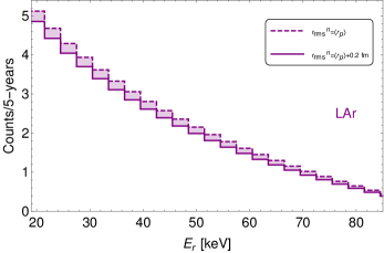
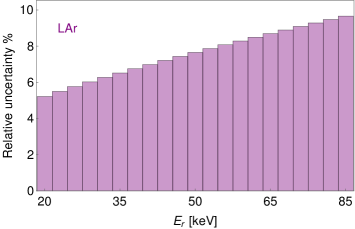
Figure 4: Recoil spectrum (left) and its relative uncertainty (right) from DSNB and atmospheric neutrinos at an Ar-based dark matter detector assuming an exposure of 1000 ton-year, as expected for Argo. The dashed (solid) histrograms correspond to $r_{\text{rms}}^{n}=r_{\text{rms}}^{p}$ ($r_{\text{rms}}^{n}=r_{\text{rms}}^{p}+0.2$ fm). The DSNB contribution is subdominant but not negligible.

Oscillations with an eV mass sterile neutrino have an effect on the CE$\nu$NS event rate. If the flux of $\nu_{\alpha}$ neutrinos ($\alpha=e,\mu,\tau$) at the source is $\Phi_{\nu_{\alpha}}(E_{\nu})$, the flux at the detector will be diminished by the fraction of neutrinos that oscillate into the sterile and the other active states. Quantitatively this means that the flux of neutrinos of flavor $\alpha$ that reach the detector is $\mathcal{P}_{\alpha\alpha}\Phi_{\nu_{\alpha}}(E_{\nu})$, where $\mathcal{P}_{\alpha\alpha}$ is the $\nu_{\alpha}$ survival probability defined as $\mathcal{P}_{\alpha\alpha}=1-\mathcal{P}_{\alpha s}-\mathcal{P}_{\alpha\beta}$ $(\alpha\neq\beta)$, with $\mathcal{P}_{\alpha s}$ and $\mathcal{P}_{\alpha\beta}$ the $\nu_{\alpha}\to\nu_{s}$ and $\nu_{\alpha}\to\nu_{\beta}$ neutrino oscillation probabilities, respectively. For short-baseline experiments $\mathcal{P}_{\alpha s}$ is given by

$$\mathcal{P}_{\alpha s}=\sin^{2}2\theta_{\alpha\alpha}\,\sin^{2}\left[1.27\left(\frac{\Delta m_{41}^{2}}{\text{eV}^{2}}\right)\left(\frac{L}{\text{m}}\right)\left(\frac{\text{MeV}}{E_{\nu}}\right)\right]\ .$$ (24)

Here, $\sin^{2}2\theta_{\alpha\alpha}=4|U_{\alpha 4}|^{2}(1-|U_{\alpha 4}|^{2})$ ($U$ is the $4\times 4$ lepton mixing matrix) and $\Delta m_{41}^{2}=m_{4}^{2}-m_{1}^{2}$ is the sterile-active neutrino mass-squared difference. The oscillation probability for active states is

$$\mathcal{P}_{\alpha\beta}=\sin^{4}\theta_{\alpha\beta}\sin^{2}\left[1.27\left(\frac{\Delta m_{41}^{2}}{\text{eV}^{2}}\right)\left(\frac{L}{\text{m}}\right)\left(\frac{\text{MeV}}{E_{\nu}}\right)\right]\ ,$$ (25)

where $\sin^{4}\theta_{\alpha\beta}=4|U_{\alpha 4}|^{2}|U_{\beta 4}|^{2}$. The recoil spectrum induced by neutrinos of flavor $\alpha$ is then given by

$$\frac{dR_{\nu_{\alpha}}}{dE_{r}}=N_{T}\sum_{\beta}\int dE_{\nu}\left[(1-\mathcal{P}_{\alpha s}-\mathcal{P}_{\alpha\beta})\Phi_{\nu_{\alpha}}+\mathcal{P}_{\alpha\beta}\Phi_{\nu_{\beta}}\right]\frac{d\sigma}{dE_{r}}\,.$$ (26)

To a fairly good approximation $\mathcal{P}_{\alpha\beta}$ can be neglected due to the higher-order active-sterile mixing suppression. $N_{T}$ is the number of target nuclei and $d\sigma/dE_{r}$ is the SM cross section in Eq. (1). The total number of counts in the $k^{\rm{th}}$ bin is obtained from Eq. (26) according to

$$R=\sum_{\alpha}R_{\nu_{\alpha}}=\sum_{\alpha}\int_{E_{k}-\Delta E_{k}}^{E_{k}+\Delta E_{k}}\,\mathcal{A}(E_{r})\,\frac{dR_{\nu_{\alpha}}}{dE_{r}}dE_{r}\ .$$ (27)

Experimental information on $R$ can then be mapped into $\sin^{2}\theta_{ij}-\Delta m_{41}^{2}$ planes.

NGI follows the same approach as NSI, but includes all possible Lorentz-invariant structures Lee and Yang (1957). It was introduced in the analysis of neutrino propagation in matter in Ref. Bergmann et al. (1999), studied in the context of CE$\nu$NS physics in Ref. Lindner et al. (2017) and in the light of COHERENT data in Ref. Aristizabal Sierra et al. (2018). Dropping flavor indices, the most general Lagrangian reads

$$\mathcal{L}_{\text{NGI}}=\frac{G_{F}}{\sqrt{2}}\sum_{\begin{subarray}{c}a=S,P,V,A,T\\ q=u,d\end{subarray}}\left[\overline{\nu}\,\Gamma^{a}\,\nu\right]\;\left[\overline{q}\,\Gamma_{a}\left(C_{a}^{q}+i\gamma_{5}\,D_{a}^{q}\right)q\right]\ ,$$ (28)

where $\Gamma_{a}=\{\mathbb{I},i\gamma_{5},\gamma_{\mu},\gamma_{\mu}\gamma_{5},\sigma_{\mu\nu}\}$, with $\sigma_{\mu\nu}=i[\gamma_{\mu},\gamma_{\nu}]/2$. As in the NSI case, some of these couplings lead to spin-suppressed interactions which we do not consider. Relevant couplings therefore include all Lorentz structures for the neutrino bilinear and only scalar, vector and tensor structures for the quark currents. For the NGI analysis, we consider only one Lorentz structure at a time and assume the $C$ and $D$ parameters to be real. We may therefore consider the individual cross sections. Assuming a spin-1/2 nuclear ground state and neglecting $\mathcal{O}(E_{r}^{2}/E_{\nu}^{2})$ terms,

$$\frac{d\sigma_{S}}{dE_{r}} =\frac{G_{F}^{2}m_{N}}{8\pi}\xi_{S}^{2}(q^{2})\frac{E_{r}m_{N}}{E_{\nu}^{2}}\ ,$$

$$\frac{d\sigma_{V}}{dE_{r}} =\frac{G_{F}^{2}m_{N}}{8\pi}\xi_{V}^{2}(q^{2})\left(2-\frac{E_{r}m_{N}}{E_{\nu}^{2}}-\frac{2E_{r}}{E_{\nu}}\right)\ ,$$

$$\frac{d\sigma_{T}}{dE_{r}} =\frac{G_{F}^{2}m_{N}}{2\pi}\xi_{T}^{2}(q^{2})\left(2-\frac{E_{r}m_{N}}{2E_{\nu}^{2}}-\frac{2E_{r}}{E_{\nu}}\right)\ .$$ (29)

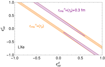
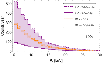
Figure 5: Left: 90% C.L. allowed regions in the NSI case and for two choices of the rms neutron radius. The diagonal bands are obtained assuming $r_{\text{rms}}^{n}=\langle r_{p}\rangle=4.79$ fm for all xenon isotopes. The purple regions are obtained for $r_{\text{rms}}^{n}=5.09$ fm (for all isotopes). Right: Number of events as a function of recoil energy for $\epsilon_{\mu\mu}^{u}\subset[-0.088,0.37]$ Coloma et al. (2017) and all other couplings equal to zero (purple histograms). The orange histograms correspond to the SM prediction including form factor uncertainties.

For the scalar and tensor cases the SM cross section has to be added. In the vector case $\xi_{V}^{2}$ includes the SM contribution which interferes with the BSM vector piece. The definition of the different parameters in Eq. (V.1) can be found in Appendix B.

V.2 Impact of neutron form factor uncertainties

We calculate the impact of uncertainties in the neutron rms radii for CsI, Ge and Xe in the presence of NSI. To do so, we take as “experimental” input the number of events predicted by the SM assuming $r_{\text{rms}}^{n}=\langle r_{p}\rangle=\sum_{i}r_{\text{rms}}^{p\,i}X_{i}=4.06$ fm for all germanium isotopes and $4.79$ fm for all xenon isotopes. Here $r_{\text{rms}}^{p\,i}$ is the rms radius of the proton distribution of the $i^{\rm{th}}$ isotope with abundance $X_{i}$. We proceed as we have done in Section IV, i.e., for CsI we take into account the Cs and I contributions, while for Ge and Xe the contributions for each isotope according to Eq. (19). For all three cases we assume four years of data taking. For our analysis we define the $\chi^{2}$ function,

$$\chi^{2}=\sum_{i}\left(\frac{N^{\text{meas}}_{i}-(1+\alpha)N^{\text{BSM}}_{i}(\mathcal{P})}{\sigma_{i}}\right)^{2}+\left(\frac{\alpha}{\sigma_{\alpha}}\right)^{2}\ ,$$ (30)

where $\alpha$ is a nuisance parameter that accounts for uncertainties in the signal rate, $N^{\text{meas}}_{i}$ is the number of simulated events in the $i^{\rm{th}}$ bin, and $N^{\text{BSM}}_{i}$ is the number of predicted events in the BSM scenario (which depend on the set of parameters $\mathcal{P}$). The statistical uncertainty in the simulated data is $\sigma_{i}=\sqrt{N_{i}^{\text{meas}}+B_{i}}$, where $B_{i}$ includes the beam-on and twice the steady-state neutron background. Beam-on neutrons are neutrons from the spallation source that penetrate the 19.3 m of moderating material, and steady-state neutrons are produced by cosmic rays interacting with the shielding material and by radioactivity. We select a 5 keV analysis threshold for the Ge and LXe detectors so that the neutron background can be assumed to be flat. It is anticipated that the shielding structures for these detectors will reduce the background rate well below the SM CE$\nu$NS expectation Akimov et al. (2018b). With that in mind, we set $\sum_{i}B_{i}$ equal to 50% of the SM signal between $5-30$ keV for the Ge and LXe detectors; this implies that the total steady-state background between $5-30$ keV is approximately 25% of the SM signal. In the future, the quenching factor uncertainty is expected to be reduced to $12.5\%$ Rich . Keeping the neutrino flux and signal acceptance uncertainties unchanged from their current values, i.e., $10\%$ and $5\%$, respectively, we have the systematic uncertainty $\sigma_{\alpha}=0.168$. Our simplification that the systematic uncertainty is correlated between bins is unavoidable given publicly available information.

Assuming $\epsilon_{\mu\mu}^{q}\subset[-1,1]$ we determine the 90% C.L. exclusion regions in two cases, $r_{\text{rms}}^{n}=\langle r_{p}\rangle$ and $r_{\text{rms}}^{n}=\langle r_{p}\rangle+0.3$ fm. We find that the CsI and Ge detectors are rather insensitive to the choice of the neutron rms radius; the resulting 90% C.L. regions barely change with $r_{\text{rms}}^{n}$. For Xe, the result is quite different. Changing $r_{\text{rms}}^{n}$ has a strong impact on the available parameter space. This can be seen from the left panel of Fig. 5, where the diagonal bands are obtained in the case $r_{\text{rms}}^{n}=\langle r_{p}\rangle$, while the purple regions are obtained for $r_{\text{rms}}^{n}=5.09$ fm. This result is as expected. Firstly, the LXe detector has a larger target mass (about a factor 6.5 larger compared to the CsI and Ge detectors), so for a common data taking time the accumulated statistics in the LXe detector is larger. Secondly, the number of events expected in the NSI scenario with $r_{\text{rms}}^{n}=\langle r_{p}\rangle$ reproduces the simulated data better than with $r_{\text{rms}}^{n}=5.09$ fm since the data are simulated with $r_{\text{rms}}^{n}=\langle r_{p}\rangle$. For the rest of our NSI study we only consider a large LXe detector. Note, however, that increasing the exposure for the CsI or Ge detectors will change the situation. In doing so these detectors will become—as the LXe detector—sensitive to uncertainties in the neutron rms radii. On the other hand, the corresponding results for a large LAr detector are not qualitatively affected by form factor uncertainties.

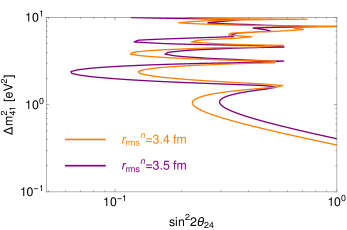
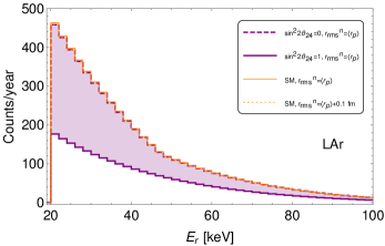
Figure 6: Left: 90% C.L. exclusion regions in the case of sterile neutrinos in the 3+1 scheme obtainable from a one ton LAr COHERENT detector with four years of data taking. The neutron rms radius is $\langle r_{p}\rangle$ for the orange contour and 3.5 fm for the purple contour. Right: The orange histograms show the SM expectation for the event spectrum including neutron form factor uncertainties, while the purple histograms are the spectra expected by fixing $r_{\text{rms}}^{n}=\langle r_{p}\rangle=3.4$ fm, $\Delta m_{41}^{2}=1.3$ eV², $\sin^{2}\theta_{14}=0.01$, $\theta_{34}=0$, with $\sin^{2}2\theta_{24}=0$ and $1$.

To determine the extent to which neutrino NSI can be distinguished from the SM signal including its neutron form factor uncertainties, we calculate the number of events assuming $\epsilon_{\mu\mu}^{d}=0$ and $\epsilon_{\mu\mu}^{u}\subset[-0.088,0.37]$. These values correspond to the 90% C.L. range obtained from global fits to neutrino oscillation data including COHERENT (CsI phase) data without accounting for energy-dependent form factor uncertainties Coloma et al. (2017). The result is shown in the right panel of Fig. 5. The NSI (purple) histograms are obtained by fixing $r_{\text{rms}}^{n}=\langle r_{p}\rangle$. The SM histograms (orange) are instead obtained by fixing $r_{\text{rms}}^{n}=\langle r_{p}\rangle$ (upper boundary) and $r_{\text{rms}}^{n}=5.09$ fm (lower boundary) and determines the SM expectation within the form factor uncertainties. Clearly, the SM expectation with form factor uncertainties lies within the NSI expectation for $\epsilon_{\mu\mu}^{u}$ between $-0.08$ and 0.2 with a fixed form factor. There are various ranges of NSI couplings that will produce signals that cannot be disentangled from the SM signal. This will persist unless uncertainties on the neutron rms radii are reduced. We have chosen $\epsilon_{\mu\mu}^{u}$ to stress this point, although results for $\epsilon_{\mu\mu}^{d}$, $\epsilon_{ee}^{q}$, $\epsilon_{\tau\tau}^{q}$ and $\epsilon_{e\tau}^{q}$, will lead to the same conclusion. Needless to say, allowing for multiple nonzero NSI parameters will further complicate the ability to discriminate new physics from the SM.

For sterile neutrinos we display the 90% C.L. exclusion regions in the $\sin^{2}2\theta_{24}-\Delta m_{41}^{2}$ plane. We highlight the exquisite sensitivity required to probe $3+1$ oscillations by assessing the capability of a future one-ton LAr COHERENT detector which has the advantage of smaller form factor uncertainties. The results for four years of data taking are shown in the left panel of Fig. 6. The analysis is similar to that for the LXe detector except that here we set $\sum_{i}B_{i}$ equal to 50% of the SM signal between $20-100$ keV. The contours are obtained for $N^{\text{BSM}}$ calculated for $r_{\text{rms}}^{n}=\langle r_{p}\rangle=3.4$ fm (orange contour) and $r_{\text{rms}}^{n}=3.5$ fm (purple contour). We fix $\sin^{2}\theta_{14}=0.01$ (best-fit value from a global fit to $\nu_{e}$ and $\bar{\nu}_{e}$ disappearance data Dentler et al. (2018)) and $\theta_{34}=0$. This result demonstrates that the available regions in parameter space have a strong dependence on the neutron rms radii. A $\sim 3\%$ change in $r_{\text{rms}}^{n}$ is sufficient to significantly modify the results of the parameter fit.

It is clear that a more precise treatment of sterile neutrino effects should include neutron form factor uncertainties, otherwise one might end up misidentifying SM uncertainties with these effects. To show this might be the case, we calculate the number of events for sterile neutrino parameters fixed as in the previous calculation and for $\Delta m_{41}^{2}=1.3$ eV², $r_{\text{rms}}^{n}=\langle r_{p}\rangle$, $\theta_{24}=0$ and $\sin^{2}2\theta_{24}=1$. We then compare the resulting (purple) histograms with the SM predictions including uncertainties (in orange); see the right panel of Fig. 6. The overlapping spectra show that an identification of the new effects is not readily possible.

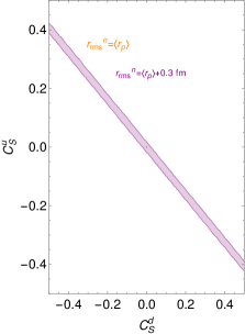
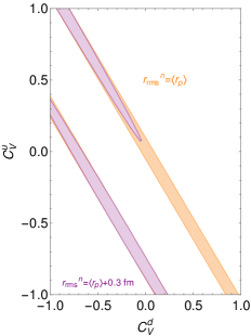
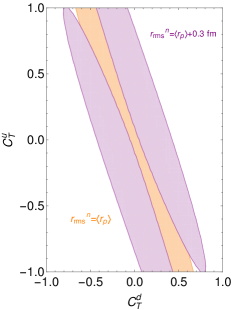
Figure 7: 90% C.L. allowed regions in the NGI parameter space for scalar interactions assuming $D_{P}^{q}=0$ (left), for vector NGI assuming $D_{A}^{q}=0$ (middle), and for tensor NGI (right). The orange bands are obtained by fixing $r_{\text{rms}}^{n}=\langle r_{p}\rangle$, while the purple regions are obtained for $r_{\text{rms}}^{n}=r_{\text{rms}}^{n}|_{\text{max}}=5.09$ fm.

Finally, we turn to the discussion of the impact of the uncertainties on the sensitivity to neutrino NGI. The results are shown in Fig. 7. We have proceeded in the same way as that for the NSI analysis, fixing $r_{\text{rms}}^{n}=\langle r_{p}\rangle$ to generate the simulated data, and analyzing the results for two cases with $r_{\text{rms}}^{n}=\langle r_{p}\rangle$ and $r_{\text{rms}}^{n}=5.09$ fm. For scalar interactions we assume $D_{P}^{q}=0$, while for vector interactions, $D_{A}^{q}=0$. Results in the case $r_{\text{rms}}^{n}=\langle r_{p}\rangle$ are quite similar to those found in Ref. Aristizabal Sierra et al. (2018) and largely depart from them for $r_{\text{rms}}^{n}=5.09$ fm for reasons similar to that for NSI. Scalar interactions are not sensitive to form factor uncertainties because fitting COHERENT data with scalar interactions leads to a rather poor fit, almost independently of $r_{\text{rms}}^{n}$. $N^{\text{meas}}$ has been simulated assuming $r_{\text{rms}}^{n}=\langle r_{p}\rangle$ and so in the presence of NGI a better fit is found for the first sample. With $r_{\text{rms}}^{n}=5.09$ fm there is little room for new interactions since the mismatch between the neutron rms radii induces substantial departure from the simulated data. Depending on the value of $r_{\text{rms}}^{n}$ large portions of parameter space are allowed or disfavored.

VI Conclusions

We have quantified the uncertainties on the SM CE$\nu$NS cross section. They are driven by the neutron form factor through its dependence on the rms radius of the neutron density distribution, $r_{\text{rms}}^{n}$. To quantify these uncertainties we assumed that $r_{\text{rms}}^{n}$ ranges between the rms radius of the proton charge distribution $r_{\text{rms}}^{p}$ of the corresponding nucleus and $r_{\text{rms}}^{p}+0.3$ fm (for heavy nuclei), so that the neutron skin is thinner than that for ${}^{208}\text{Pb}$ (which has been measured by PREX). For nuclei with $N\sim Z$, we considered $r_{\text{rms}}^{n}$ between $r_{\text{rms}}^{p}$ and $r_{\text{rms}}^{p}+0.1$ fm or $r_{\text{rms}}^{p}+0.2$ fm. Under this assumption we evaluated the size of the uncertainties for ${}^{133}\text{Cs}$, ${}^{127}\text{I}$, germanium, xenon and argon—choices motivated by COHERENT phases I-III and Argo—using three form factor parameterizations: Helm, Fourier transform of the symmeterized Fermi function and Klein-Nystrand.

We showed that form factor uncertainties: (i) are relevant for $q\gtrsim 20\,$MeV, and so are negligible if the CE$\nu$NS process is induced by either reactor or solar neutrinos, (ii) have percentage uncertainties that have a strong dependence on the recoil energy (iii) are basically independent of the parameterization used.

We studied the impact of the uncertainties on the SM prediction for COHERENT, diffuse supernova neutrino background, and sub-GeV atmospheric neutrinos. For COHERENT, assuming $n_{\text{POT}}$/year as in Ref. Akimov et al. (2017), we found that the SM prediction is subject to relative uncertainties that are never below $1.5\%$ in germanium, $2\%$ is argon and $6\%$ in xenon. For the combination of DSNB and atmospheric neutrinos we find that the relative uncertainties are at least $5\%$. These results demonstrate that in the absence of precise measurements of $r_{\text{rms}}^{n}$, SM predictions of the CE$\nu$NS rate involve uncertainties that challenge the interpretation of data. This is especially true for future measurements with small experimental systematic uncertainties.

We also quantified the impact of the neutron form factor uncertainties on the sensitivity to new physics. We considered three scenarios: neutrino NSI, sterile neutrinos in the 3+1 scheme, and NGI. We showed that the variation of $r_{\text{rms}}^{n}$ has a substantial effect on these new physics searches with the exception of scalar NGI for which we did not find any sensitivity.

Finally, it is worth pointing out that the uncertainties we have derived here also apply to DM direct detection searches, provided the WIMP-nucleus interactions are spin independent. In WIMP scenarios with vector, scalar and tensor mediators, the direct detection rate will involve uncertainties comparable to those we have derived.

Appendix A Diffuse supernova neutrino background fluxes

For the calculation of the DSNB neutrino flux we closely follow Ref. Horiuchi et al. (2009). Here we present the details of such a calculation. The predicted DSNB flux is obtained by integrating the rate of core-collapse supernova, $R_{\text{SN}}(z)$, multiplied by the neutrino emission per supernova, $dN(E_{\nu}^{\prime})/dE_{\nu}^{\prime}$, redshifted over cosmic time:

$$\frac{d\Phi(E_{\nu})}{dE_{\nu}}=\frac{4\pi\,c}{H_{0}}\,\int_{0}^{z_{\text{max}}}\,R_{\text{SN}}(z)\,\frac{dN_{\nu_{i}}(E_{\nu}^{\prime})}{dE_{\nu}^{\prime}}\,\frac{dz}{\sqrt{\Omega_{m}(1+z)^{3}+\Omega_{\Lambda}}}\ .$$ (31)

Here the redshifted neutrino energy is given by $E_{\nu}^{\prime}=(1+z)E_{\nu}$, and $z_{\text{max}}$ is determined by gravitational collapse, assumed to start at $z=5$ Ando and Sato (2004). The cosmological parameters have been fixed to: $\Omega_{m}=0.3$, $\Omega_{\Lambda}=0.7$ and $H_{0}=70\,\text{km}\,\text{s}^{-1}\,\text{Mpc}^{-1}$. The rate for core-collapse supernova in units of Mpc^-3year^-1 is determined by the star formation rate $\dot{\rho}_{*}(z)$ and the initial mass function $\Psi(M)$ as

$$R_{\text{SN}}(z)=\dot{\rho}_{*}(z)\,\frac{\int_{8\text{M}_{\odot}}^{150\text{M}_{\odot}}\Psi(M)dM}{\int_{0.1\text{M}_{\odot}}^{100\text{M}_{\odot}}M\Psi(M)dM}\ .$$ (32)

The integral in the numerator gives the number of stars that produce core collapse supernova, while the integral in the denominator gives the total mass in stars. The initial mass function $\Psi(M)=dN/dM$ determines the number of stars with masses in the range $M$ and $M+dM$ and reads $\Psi(M)=M^{-\xi}$, with the value of $\xi$ defining a particular initial mass function and therefore the value of the integrals in (32). For our calculation we have used a Baldry-Glazebrook initial mass function Baldry and Glazebrook (2003) for which the integral has a value of $0.0132/\text{M}_{\odot}$. The star formation rate is given by the fitted function

$$\dot{\rho}_{*}(z)=\dot{\rho}_{0}\left[(1+z)^{\alpha\eta}+\left(\frac{1+z}{B}\right)^{\beta\eta}+\left(\frac{1+z}{C}\right)^{\gamma\eta}\right]^{1/\eta}\ ,$$ (33)

where $\eta=10$ and the constants $B$ and $C$ are

$$B=(1+z_{1})^{1-\alpha/\beta}\ ,\qquad C=(1+z_{1})^{(\beta-\alpha)/\gamma}(1+z_{2})^{1-\beta/\gamma}\,.$$ (34)

We fix $\alpha=3.4$, $\beta=-0.3$, $\gamma=-3.5$, $z_{1}=1$, $z_{2}=4$ and $\dot{\rho}_{0}=0.0178\,\text{M}_{\odot}\text{year}^{-1}\text{Mpc}^{-3}$, which correspond to the fiducial analytic fit given in Ref. Horiuchi et al. (2009).

In core-collapse supernova, neutrinos of all flavors are emitted and each flavor carries about the same fraction of the total energy, $E_{\nu}\simeq 3\times 10^{53}$ erg. Their spectra are approximately thermal with temperatures obeying $T_{\bar{\nu}_{e}}<T_{\nu_{e}}<T_{\nu_{x}}$ ($\nu_{x}=\nu_{\mu},\nu_{\tau},\bar{\nu}_{\mu},\bar{\nu}_{\tau}$). We have taken a Fermi-Dirac distribution with zero chemical potential for all flavors,

$$\frac{dN_{\nu_{i}}(E^{\prime}_{\nu})}{dE_{\nu}}=\frac{E_{\nu}^{\text{tot}}}{6}\frac{120}{7\pi^{4}}\frac{E_{\nu_{i}}^{{}^{\prime}2}}{T_{\nu_{i}}}\frac{1}{e^{E_{\nu_{i}}^{\prime}/T_{\nu_{i}}}+1}\ ,$$ (35)

and temperatures according to: $T_{\bar{\nu}_{e}}=3$ MeV, $T_{\nu_{e}}=5$ MeV and $T_{\nu_{x}}=8$ MeV.

Appendix B NGI cross section parameters

The parameters in Eq. (V.1) are closely related to those in Ref. Aristizabal Sierra et al. (2018), but involve a $q^{2}$ dependence related to the proton and neutron form factors. For the $\xi_{X}$ ($X=S,V,T$) couplings we have

$$\xi_{S}^{2}(q^{2}) =C_{S}^{2}(q^{2})+D_{P}^{2}(q^{2})\ ,\qquad\xi_{T}^{2}(q^{2})=2C_{T}^{2}(q^{2})\ ,$$

$$\xi_{V}^{2}(q^{2}) =\left[C_{V}^{2}(q^{2})+2g_{V}(q^{2})\right]^{2}+D_{A}^{2}(q^{2})\ ,$$ (36)

with $g_{V}=g_{V}^{n}F_{n}(q^{2})+g_{V}^{p}F_{p}(q^{2})$. In the scalar case, the parameters that define $\xi_{S}$ read

$$C_{S}(q^{2})=\sum_{q=u,d}C_{s}^{(q)}\left[N\frac{m_{n}}{m_{q}}f_{T_{q}}^{n}F_{n}(q^{2})+Z\frac{m_{p}}{m_{q}}f_{T_{q}}^{p}F_{p}(q^{2})\right]\ ,$$ (37)

and the same definition applies for $D_{P}(q^{2})$ by trading $C_{S}^{(q)}\to D_{P}^{(q)}$. The parameters $f_{T_{q}}$ are derived in chiral perturbation theory from measurements of the $\pi$-nucleon sigma term Cheng (1989). For our calculations we use the values

$$f_{T_{u}}^{p} =0.019\ ,\qquad f_{T_{d}}^{p}=0.041\ ,$$

$$f_{T_{u}}^{n} =0.023\ ,\qquad f_{T_{d}}^{n}=0.034\ .$$ (38)

For the vector coupling $\xi_{V}$ we have

$$C_{V}(q^{2})=N(C_{V}^{u}+2C_{V}^{d})F_{n}(q^{2})+Z(2C_{V}^{u}+C_{V}^{d})F_{p}(q^{2})\ .$$ (39)

The expression for $D_{A}(q^{2})$ can be obtained from (39) by trading $C_{V}^{q}\to D_{A}^{q}$ with $q=u,\,d$. Finally, in the tensor case,

$$C_{T}(q^{2})=N(\delta_{u}^{n}C_{T}^{u}+\delta_{d}^{n}C_{T}^{d})F_{n}(q^{2})+Z(\delta_{u}^{p}C_{T}^{u}+\delta_{d}^{p}C_{T}^{d})F_{p}(q^{2})\ .$$ (40)

For $\delta_{q}^{n}$ and $\delta_{q}^{p}$ we use values obtained from azimuthal asymmetries in semi-inclusive deep-inelastic scattering and $e^{+}e^{-}\to h_{1}h_{2}X$ Anselmino et al. (2009); more up-to-date values can be found in Courtoy et al. (2015); Goldstein et al. (2014); Radici et al. (2015). For our calculation we use

$$\delta_{u}^{p} =0.54\ ,\qquad \delta_{d}^{p}=-0.23\ ,$$

$$\delta_{u}^{n} =-0.23\ ,\qquad \delta_{d}^{n}=0.54\ .$$ (41)

References

- Akimov et al. (2017) D. Akimov et al. (COHERENT), Science (2017), eprint 1708.01294.
- Cañas et al. (2018) B. C. Cañas, E. A. Garcés, O. G. Miranda, and A. Parada, Phys. Lett. B784, 159 (2018), eprint 1806.01310.
- Patton et al. (2012) K. Patton, J. Engel, G. C. McLaughlin, and N. Schunck, Phys. Rev. C86, 024612 (2012), eprint 1207.0693.
- Barranco et al. (2005) J. Barranco, O. G. Miranda, and T. I. Rashba, JHEP 12, 021 (2005), eprint hep-ph/0508299.
- Scholberg (2006) K. Scholberg, Phys. Rev. D73, 033005 (2006), eprint hep-ex/0511042.
- Coloma et al. (2017) P. Coloma, M. C. Gonzalez-Garcia, M. Maltoni, and T. Schwetz, Phys. Rev. D96, 115007 (2017), eprint 1708.02899.
- Liao and Marfatia (2017) J. Liao and D. Marfatia, Phys. Lett. B775, 54 (2017), eprint 1708.04255.
- Papoulias and Kosmas (2018) D. K. Papoulias and T. S. Kosmas, Phys. Rev. D97, 033003 (2018), eprint 1711.09773.
- Billard et al. (2018) J. Billard, J. Johnston, and B. J. Kavanagh, JCAP 1811, 016 (2018), eprint 1805.01798.
- Aristizabal Sierra et al. (2018) D. Aristizabal Sierra, V. De Romeri, and N. Rojas, Phys. Rev. D98, 075018 (2018), eprint 1806.07424.
- Cadeddu et al. (2018a) M. Cadeddu, C. Giunti, K. A. Kouzakov, Y. F. Li, A. I. Studenikin, and Y. Y. Zhang, Phys. Rev. D98, 113010 (2018a), eprint 1810.05606.
- Helm (1956) R. H. Helm, Phys. Rev. 104, 1466 (1956).
- Sprung and Martorell (1997) D. W. L. Sprung and J. Martorell, Journal of Physics A: Mathematical and General 30, 6525 (1997), URL http://stacks.iop.org/0305-4470/30/i=18/a=026.
- Klein and Nystrand (1999) S. Klein and J. Nystrand, Phys. Rev. C60, 014903 (1999), eprint hep-ph/9902259.
- Lewin and Smith (1996) J. D. Lewin and P. F. Smith, Astropart. Phys. 6, 87 (1996).
- Angeli and Marinova (2013) I. Angeli and K. P. Marinova, Atom. Data Nucl. Data Tabl. 99, 69 (2013).
- Akimov et al. (2018a) D. Akimov et al. (COHERENT) (2018a), eprint 1804.09459.
- Aalseth et al. (2018) C. E. Aalseth et al., Eur. Phys. J. Plus 133, 131 (2018), eprint 1707.08145.
- Akimov et al. (2015) D. Akimov et al. (COHERENT) (2015), eprint 1509.08702.
- Freedman (1974) D. Z. Freedman, Phys. Rev. D9, 1389 (1974).
- Freedman et al. (1977) D. Z. Freedman, D. N. Schramm, and D. L. Tubbs, Ann. Rev. Nucl. Part. Sci. 27, 167 (1977).
- Tishchenko et al. (2013) V. Tishchenko et al. (MuLan), Phys. Rev. D87, 052003 (2013), eprint 1211.0960.
- Tanabashi et al. (2018) M. Tanabashi et al. (Particle Data Group), Phys. Rev. D98, 030001 (2018).
- Billard et al. (2014) J. Billard, L. Strigari, and E. Figueroa-Feliciano, Phys. Rev. D89, 023524 (2014), eprint 1307.5458.
- Abrahamyan et al. (2012) S. Abrahamyan et al., Phys. Rev. Lett. 108, 112502 (2012), eprint 1201.2568.
- Horowitz et al. (2012) C. J. Horowitz et al., Phys. Rev. C85, 032501 (2012), eprint 1202.1468.
- Horowitz et al. (2014) C. J. Horowitz, K. S. Kumar, and R. Michaels, Eur. Phys. J. A50, 48 (2014), eprint 1307.3572.
- Cadeddu et al. (2018b) M. Cadeddu, C. Giunti, Y. F. Li, and Y. Y. Zhang, Phys. Rev. Lett. 120, 072501 (2018b), eprint 1710.02730.
- (29) J. Piekarewicz, private communication.
- Piekarewicz et al. (2016) J. Piekarewicz, A. R. Linero, P. Giuliani, and E. Chicken, Phys. Rev. C94, 034316 (2016), eprint 1604.07799.
- Ando and Sato (2004) S. Ando and K. Sato, New J. Phys. 6, 170 (2004), eprint astro-ph/0410061.
- Horiuchi et al. (2009) S. Horiuchi, J. F. Beacom, and E. Dwek, Phys. Rev. D79, 083013 (2009), eprint 0812.3157.
- Battistoni et al. (2005) G. Battistoni, A. Ferrari, T. Montaruli, and P. R. Sala, Astropart. Phys. 23, 526 (2005).
- Ferrari et al. (2005) A. Ferrari, P. R. Sala, A. Fasso, and J. Ranft (2005).
- Wolfenstein (1978) L. Wolfenstein, Phys. Rev. D17, 2369 (1978).
- Lee and Yang (1957) T. D. Lee and C.-N. Yang, Phys. Rev. 105, 1671 (1957), [245(1957)].
- Bergmann et al. (1999) S. Bergmann, Y. Grossman, and E. Nardi, Phys. Rev. D60, 093008 (1999), eprint hep-ph/9903517.
- Lindner et al. (2017) M. Lindner, W. Rodejohann, and X.-J. Xu, JHEP 03, 097 (2017), eprint 1612.04150.
- Akimov et al. (2018b) D. Akimov et al. (COHERENT) (2018b), eprint 1803.09183.
- (40) G. Rich, private communication.
- Dentler et al. (2018) M. Dentler, A. Hernández-Cabezudo, J. Kopp, P. A. N. Machado, M. Maltoni, I. Martinez-Soler, and T. Schwetz, JHEP 08, 010 (2018), eprint 1803.10661.
- Baldry and Glazebrook (2003) I. K. Baldry and K. Glazebrook, Astrophys. J. 593, 258 (2003), eprint astro-ph/0304423.
- Cheng (1989) H.-Y. Cheng, Phys. Lett. B219, 347 (1989).
- Anselmino et al. (2009) M. Anselmino, M. Boglione, U. D’Alesio, A. Kotzinian, F. Murgia, A. Prokudin, and S. Melis, Nucl. Phys. Proc. Suppl. 191, 98 (2009), eprint 0812.4366.
- Courtoy et al. (2015) A. Courtoy, S. Baeßler, M. González-Alonso, and S. Liuti, Phys. Rev. Lett. 115, 162001 (2015), eprint 1503.06814.
- Goldstein et al. (2014) G. R. Goldstein, J. O. Gonzalez Hernandez, and S. Liuti (2014), eprint 1401.0438.
- Radici et al. (2015) M. Radici, A. Courtoy, A. Bacchetta, and M. Guagnelli, JHEP 05, 123 (2015), eprint 1503.03495.