Quantum convolutional data-syndrome codes

Abstract

We consider performance of a simple quantum convolutional code in a fault-tolerant regime using several syndrome measurement/decoding strategies and three different error models, including the circuit model.

I Introduction

Quantum stabilizer codes are designed to be robust against qubit errors. However, syndrome measurement cannot be done perfectly: necessarily, there are some measurement errors whose probability grows with the weight of the checks (stabilizer generators). Furthermore, both the syndrome measurement protocol and the syndrome-based decoding have to operate in a fault-tolerant (FT) regime, to be robust against errors that happen during the measurement.

When all checks have relatively small weights, as in the case of the surface codes, one simple approach is to repeat syndrome measurement several times[1]. Then, FT syndrome-based decoding can be done in the assumption that the data errors accumulate while measurement errors be independently distributed. While there is always a non-vanishing probability to have some errors at the end of the cycle, what matters in practice is the ability to backtrack all errors after completion of several rounds of measurement.

Another approach it to measure an overcomplete set of stabilizer generators, using redundancy to recover the correct syndrome. Such an approach was used in the context of higher-dimensional toric and/or color codes[2, 3], the data-syndrome (DS) codes[4, 5, 6], and single-shot measurement protocols[7, 8, 9]. Here decoding is done in the assumption that data error remains the same during the measurement.

We note that with both approaches, the error models assumed for decoding do not exactly match the actual error probability distribution. In particular, any correlations between errors in different locations and/or different syndrome bits are typically ignored. Nevertheless, simulations with circuit-based error models which reproduce at least some of the actual correlations show that both the repeated syndrome measurement protocol[10, 11] and the syndrome measurement protocols relying on an overcomplete set of generators[3] can result in competitive values of FT threshold.

The choice of the measurement protocol is typically dictated by the structure of the code, specifically, availability of an overcomplete set of stabilizer generators of the minimum weight. Such an approach is expected to be practical when typical gate infidelities are comparable with the probability of an incorrect qubit measurement. However, there is also a price to pay: codes with redundant sets of small-weight checks can be generally expected to have worse parameters.

On the other hand, if the physical one- and two-qubit gates are relatively accurate, it may turn out more practical to measure redundant sets of checks which include stabilizer generators of higher weights. Then, a DS code can be designed from any stabilizer code[4, 5, 6]. As a result, one faces a problem of constructing an optimal measurement protocol given the known gate fidelities and measurement errors.

In this work we compare several single-shot and repeated measurement/decoding protocols for a simple quantum convolutional code[12] with the parameters $[[24,6,3]]$ and syndrome generators of weight 6. We construct several computationally efficient schemes using the classical Viterbi algorithm[13, 14] to decode data and syndrome errors sequentially or simultaneously, and compare their effectiveness both with phenomenological and circuit-based depolarizing error models. In particular, we show that a DS code which requires measuring checks of weight up to $w_{\mathrm{max}}=9$ has performance (successful decoding probability) exceeding that of the repeated measurement scheme when single-qubit measurement error probability $q_{1}$ equals ten times the gate error probability $p_{1}$ (taken to be the same for Hadamard and CNOT gates).

II Background

Let $\mathcal{P}_{n}=\{c\,M_{1}\otimes\cdots\otimes M_{n}:M_{j}\in\{I,X,Y,Z\}\}$, with phase $c\in\{\pm 1,\pm i\}$ be the $n$-qubit Pauli group; elements with $c=\pm 1$ have eigenvalues $\pm 1$. Any $G=c\,M_{1}\otimes\cdots\otimes M_{n}\in\mathcal{P}_{n}$ can be represented, up to a phase, by length-$n$ vector ${\bf g}=(g_{1},\ldots,g_{n})\in\mathbb{F}_{4}^{n},~{}\mathbb{F}_{4}=\{0,1,\omega,\bar{\omega}\}$, where $\omega^{2}\equiv\bar{\omega}=\omega+1$, and $g_{j}=0,1,\omega,\bar{\omega}$, if $M_{j}$ is $I$, $X$, $Z$, or $Y$, respectively. The weight $\mathop{\mathrm{wt}}({\bf g})$ of ${\bf g}$ is the number of its nonzero elements $g_{j}\not=0$. A product of two Pauli operators $X$ and $Y$ is mapped into a sum of the corresponding vectors, ${\bf x}+{\bf y}$. Further, a pair of Pauli operators commute iff the trace inner product,

$${\bf x}*{\bf y}^{T}\equiv\sum\nolimits_{i=1}^{n}\mathop{\mathrm{Tr}}(x_{i}\bar{y}_{i}),$$ (1)

of the corresponding vectors is zero, ${\bf x}*{\bf y}^{T}=0$. Here $\mathop{\mathrm{Tr}}(x)=x+x^{2}$ is the trace map from $\mathbb{F}_{4}$ into $\mathbb{F}_{2}$, and $\bar{y}$ is the conjugation of $y\in\mathbb{F}_{4}$ which interchanges $\omega$ and $\bar{\omega}$.

An $[[n,k]]$ quantum stabilizer code ${\cal Q}$, a subspace of the $n$-qubit Hilbert space, encodes $k$ qubits into $n$, and its rate is defined as $R=k/n$. Any code vector (quantum state) $\left|\psi\right\rangle\in{\cal Q}$ is stabilized by a stabilizer group ${\cal S}$, an Abelian subgroup of $\mathcal{P}_{n}$ such that $-I^{\otimes n}\not\in{\cal S}$. Such a subgroup is mapped to an additive code ${\cal C}$ of size $|{\cal C}|=2^{n-k}$ over $\mathbb{F}_{4}$, specified by the generator matrix ${\bf G}$ whose rows ${\bf g}_{j}$ correspond to the Pauli generators $G_{j}\in{\cal S}$. The additivity means that for any ${\bf x},{\bf y}\in{\cal C}$ we have ${\bf x}+{\bf y}\in{\cal C}$. A detectable error $E\in{\cal P}_{n}$ has non-zero commutators with one or more generators of ${\cal S}$; the corresponding vector ${\bf e}\in\mathbb{F}_{4}^{n}$ has a non-zero syndrome ${\bf s}^{T}={\bf G}*{\bf e}^{T}$. Vectors corresponding to undetectable errors form the dual (with respect to the trace inner product) code ${\cal C}^{\perp}$ of size $|{\cal C}^{\perp}|=2^{n+k}$. Since ${\cal S}$ is Abelian, one necessarily has ${\cal C}\subseteq{\cal C}^{\perp}$, and for this reason ${\cal C}$ is called self-orthogonal. Elements of ${\cal S}$ act trivially on the code ${\cal Q}$; thus the distance $d$ of a quantum code is defined as the minimum weight of an element of ${\cal C}^{\perp}\setminus{\cal C}$ [15].

For numerics in this work we use the family of quantum convolutional codes (QCCs) of length $3(k+2)$, $k=1,2,\ldots$, based on linear $(3,1)$ self-orthogonal convolutional codes whose generator matrces are constructed[12] by $k+1$ shifts of the row ${\bf g}_{1}=(111|1\omega\bar{\omega})$. The actual generating matrix of the QCC ${\cal Q}_{k}$ with parameters $[[3(k+2),k,3]]$ is obtained by adding a copy of the same rows multiplied by $\omega$, and four additional rows for proper termination. In the case $k=1$, the stabilizer generating matrix has the form

$${\bf G}({\cal Q}_{1})=\left(\begin{array}[]{ccc|ccc|ccc}1&\omega&\overline{\omega}&&&\\ \overline{\omega}&\omega&1&&&\\ 1&1&1&1&\omega&\overline{\omega}\\ \omega&\omega&\omega&\omega&\overline{\omega}&1\\ &&&1&1&1&1&\omega&\overline{\omega}\\ &&&\omega&\omega&\omega&\omega&\overline{\omega}&1\\ &&&&&&\overline{\omega}&\omega&1\\ &&&&&&1&1&1\\ \end{array}\right).$$ (2)

III Error models and data-syndrome codes

Unlike with classical codes, extracting a syndrome for a quantum code involves a complicated quantum measurement which itself is prone to errors. To extract a syndrome bit corresponding to a row ${\bf g}$ of ${\bf G}$, one must execute a unitary which involves a non-trivial interaction [some single-qubit gate(s) and an entangling gate, e.g., a quantum CNOT] with each of the $w\equiv\mathop{\mathrm{wt}}({\bf g})$ qubits in the support of ${\bf g}$, then do a quantum measurement of one or more auxiliary ancilla qubit(s). Data errors and measurement (ancilla) errors can happen at every step of the process; moreover, errors can propagate through measurement circuit unless it is designed using FT gadgets to prevent error multiplication[16]. Error propagation can be simulated efficiently for any circuit constructed from Clifford gates which map the Pauli group onto itself, which is sufficient to simulate the performance of any stabilizer code[17]. In this work we simulated such a circuit-based error model (C), using depolarizing noise with probability $p_{1}$ (randomly chosen $X$, $Y$, or $Z$ on every qubit in the interval between subsequent gates, including null gates for idle qubits), and additional ancilla measurement error with probability $q_{1}$ [10, 11].

While in principle it is possible to account for all correlations between the errors that may result from error propagation in a given circuit, and design a corresponding decoder, it would be a daunting task. Instead, one usually uses a decoder designed for some phenomenological error model, and uses circuit model (C) only to check the performance of such a decoder numerically. We consider two such error models.

Model (A) is a channel model where qubit errors (depolarizing noise with probability $p$) happen before the measurement, while each stabilizer generator (syndrome bit) is measured with independent error probability $q$. This model[5, 6] is an idealization of a situation where gate errors are small compared to qubit preparation and measurement errors. Clearly, model (A) can get unphysical, as here one can extract the syndrome perfectly with sufficient measurement redundancy.

This drawback is compensated somewhat in the phenomenological error model (B) which includes several rounds of syndrome measurement, and includes qubit errors that happen before each round (depolarizing noise with probability $p$; these errors accumulate between measurement rounds), and independent syndrome measurement errors with probability $q$. Both in the phenomenological model (B) and in the circuit model (C) some errors may remain after the last round of error correction; for simulations one includes an additional round with perfect syndrome measurement[10].

Phenomenological error models (A) and (B) can be used to construct DS codes dealing both with qubit (data) and syndrome errors. We start with an $r\times n$ stabilizer generator matrix ${\bf G}$, which may include additional linearly-dependent rows, thus $r\geq n-k$. In model (A), we have a qubit error vector ${\bf e}\in\mathbb{F}_{2}^{n}$, and a syndrome measurement error $\boldsymbol{\epsilon}\in\mathbb{F}_{2}^{r}$; the extracted syndrome vector is given by ${\bf s}^{T}={\bf G}*{\bf e}^{T}+\boldsymbol{\epsilon}^{T}$. To characterize DS codes, it is convenient to consider mixed-field vector spaces, with elements $\left({\bf e}\,|\,\boldsymbol{\epsilon}\right)$, a pair of a quaternary and a binary vectors. For such pairs we define the inner product

$$({\bf e}_{1},\boldsymbol{\epsilon}_{1})\star({\bf e}_{2},\boldsymbol{\epsilon}_{2})^{T}\equiv{\bf e}_{1}*{\bf e}_{2}^{T}+\boldsymbol{\epsilon}_{1}\boldsymbol{\epsilon}_{2}^{T}.$$ (3)

By analogy with stabilizer codes, we define an additive code ${\cal C}_{\rm DS}\subseteq\mathbb{F}_{4}^{n}\oplus\mathbb{F}_{2}^{r}$ with the generator matrix

$${\bf G}_{\rm DS}=\left(\begin{array}[c]{c|c}{\bf G}&{\bf I}\end{array}\right),$$ (4)

and its dual with respect to the product (3), ${\cal C}_{\rm DS}^{\perp}$. The two orthogonal DS codes satisfy $|{\cal C}_{\rm DS}|\,|{\cal C}_{\rm DS}^{\perp}|=2^{2n+r}$. Because the original code ${\cal C}$ is self orthogonal, ${\bf G}*{\bf G}^{T}=0$, the code ${\cal C}_{\rm DS}^{\perp}$ includes vectors in the form $({\bf e}\,|\,{\bf 0})$, where ${\bf e}=\boldsymbol{\alpha}{\bf G}$ is an additive combination of the rows of ${\bf G}$, $\boldsymbol{\alpha}\in\mathbb{F}_{2}^{r}$. The distance $d_{\rm DS}$ of thus defined DS code is the minimum weight of a vector in ${\cal C}_{\rm DS}^{\perp}\setminus({\cal C}\oplus{\bf 0})$, it is upper bounded by the distance of the original quantum code ${\cal Q}$, $d_{\rm DS}\leq d$.

In phenomenological error model (B), with $\ell$-times repeated syndrome measurement (including the final perfect measurement), we denote qubit errors that occur before the measurement $t$ as ${\bf e}_{t}\in\mathbb{F}_{4}^{n}$, and the corresponding measurement errors as $\boldsymbol{\epsilon}_{t}\in\mathbb{F}_{2}^{r}$. The qubit errors accumulate, thus we can write for the syndrome ${\bf s}_{t}$ obtained in the $t$ th round of measurement:

$${\bf G}*({\bf e}_{1}+{\bf e}_{2}+\ldots+{\bf e}_{t})+\boldsymbol{\epsilon}_{t} = {\bf s}_{t}.$$

In this work we do not attempt simultaneous decoding of data and syndrome errors over several rounds of measurement. Instead we decode them sequentially, using the accumulated errors $\hat{{\bf e}}_{1}+\hat{{\bf e}}_{2}+\ldots+\hat{{\bf e}}_{t-1}$ extracted at previous decoding rounds to offset the error at time $t$.

IV Convolutional DS codes

Now, given an $[[n,k]]$ quantum code ${\cal Q}$ with the (full-row-rank) generating matrix ${\bf G}({\cal Q})$ of size $(n-k)\times n$, we introduce redundant measurements by adding some linearly dependent rows. Without limiting generality, a set of $r^{\prime}$ additional rows ${\bf F}={\bf A}{\bf G}({\cal Q})$ can be obtained by multiplying the original generating matrix by an $r^{\prime}\times(n-k)$ binary matrix ${\bf A}$, so that the generating matrix 5 of the resulting DS code has the form

$${\bf G}_{\rm DS}=\left(\begin{array}[c]{c|cc}{\bf G}({\cal Q})&{\bf I}_{n-k}&\\ {\bf A}{\bf G}({\cal Q})&&{\bf I}_{r^{\prime}}\end{array}\right).$$ (5)

This matrix has additive rank $r\equiv(n-k)+r^{\prime}$ equal to the number of rows. It is convenient to rewrite this matrix in the following row-equivalent form,

$${\bf G}_{\rm DS}^{\prime}=\left(\begin{array}[c]{c|cc}{\bf G}({\cal Q})&{\bf I}_{n-k}&\\ &{\bf A}&{\bf I}_{r^{\prime}}\end{array}\right).$$ (6)

Denote $[{\bf G}({\cal Q})]^{\perp}$ the additive dual of ${\bf G}({\cal Q})$ with additive rank $n+k$, and ${\bf M}$ a matrix such that ${\bf G}({\cal Q})\,{\bf M}^{T}={\bf I}_{n-k}$. It is then easy to see that the matrix

$${\bf H}_{\rm DS}=\left(\begin{array}[c]{c|cc}[{\bf G}({\cal Q})]^{\perp}&&\\ {\bf M}&{\bf I}_{n-k}&{\bf A}^{T}\end{array}\right).$$ (7)

has additive rank $(n+k)+(n-k)=2n$, while ${\bf G}_{\rm DS}^{\prime}\star{\bf H}_{\rm DS}^{T}=0$. Thus, ${\bf H}_{\rm DS}$ generates the code ${\cal C}_{DS}^{\perp}$.

We can now discuss the choice of the matrix ${\bf A}$. First, we obtain redundant syndrome bits by measuring operators $F_{j}$ corresponding to the rows ${\bf f}_{j}$ of the matrix ${\bf F}$. Since the corresponding error grows with the operator weight, we want to choose matrix ${\bf A}$ to ensure that row weights of ${\bf F}$ be small. Second, we want to choose ${\bf A}$ so that the binary linear code generated by $({\bf I}_{n-k},{\bf A}^{T})$ has a large minimum distance. Third important issue is the decoding complexity. Given the structure of the matrix ${\bf H}_{\rm DS}$, see Eq. (7), it is natural to choose ${\bf A}^{T}$ to form a generator matrix of a classical convolutional code. Quantum DS codes (5) obtained from a quantum convolutional code ${\cal Q}$ with such an ${\bf A}$ we call convolutional DS codes.

V Decoding of Convolutional DS Codes

Big advantage of classical convolutional codes is that one can use the maximum-likelihood Viterbi decoding using a code trellis [14]. The “stripe” form of a generator matrix of a convolutional code (with small band width) ensures that its code trellis has relatively small number of states, which means that the Viterbi decoding has relatively small complexity.

In our case, it is not immediately obvious how to construct a code trellis with a manageable number of states, since neither ${\bf G}_{\rm DS}$ nor ${\bf H}_{\rm DS}$ has the “stripe” form. However, we show that ${\bf G}_{\rm DS}$ can be transformed into the stripe form.

Instead of presenting a general algorithm for this, we will consider a small example. Let ${\bf G}({\cal Q})$ and ${\bf A}$ be generated by vectors $({\bf v}_{1}|{\bf v}_{2}|{\bf v}_{3})$ and $({\bf u}_{1}|{\bf u}_{2}|{\bf u}_{3})$, respectively, and assume that ${\bf v}_{i}$ and ${\bf u}_{i}$ have lengths $n$ and $n^{\prime}$. Then, in a particular case, the DS code generator (6) has the form

$${\bf G}_{\rm DS}^{\prime}=$$

$$\left(\begin{array}[]{cccc ccc cccccc}{\bf v}_{1}&{\bf v}_{2}&{\bf v}_{3}&&&1&&&&&&&\\ &{\bf v}_{1}&{\bf v}_{2}&{\bf v}_{3}&&&1&&&&&&\\ &&{\bf v}_{1}&{\bf v}_{2}&{\bf v}_{3}&&&1&&&&&\\ &&&&&{\bf u}_{1}^{T}&&&{\bf I}&&&&\\ &&&&&{\bf u}_{2}^{T}&{\bf u}_{1}^{T}&&&{\bf I}&&&\\ &&&&&{\bf u}_{3}^{T}&{\bf u}_{2}^{T}&{\bf u}_{1}^{T}&&&{\bf I}&&\\ &&&&&&{\bf u}_{3}^{T}&{\bf u}_{2}^{T}&&&&{\bf I}&\\ &&&&&&&{\bf u}_{3}^{T}&&&&&{\bf I}\end{array}\right),$$

where ${\bf I}$ is the $n^{\prime}\times n^{\prime}$ identity matrix. With an appropriate permutation of columns and rows, we can transform the above matrix into the form

$${\bf G}_{\rm DS}^{\prime\prime}=$$

$$\left(\begin{array}[]{cccc|ccc|cccccc}\cline{5-7}\cr{\bf v}_{1}&{\bf v}_{2}&&&{\bf v}_{3}&1&&\\ &&{\bf I}&&&{\bf u}^{T}_{1}&&\\ &{\bf v}_{1}&&&{\bf v}_{2}&&&{\bf v}_{3}&1\\ &&&{\bf I}&&{\bf u}^{T}_{2}&&&{\bf u}^{T}_{1}\\ &&&&{\bf v}_{1}&&&{\bf v}_{2}&&&{\bf v}_{3}&1\\ &&&&&{\bf u}^{T}_{3}&{\bf I}&&{\bf u}^{T}_{2}&&&{\bf u}^{T}_{1}\\ \cline{5-7}\cr&&&&&&&&{\bf u}^{T}_{3}&{\bf I}&&{\bf u}^{T}_{2}&\\ &&&&&&&&&&&{\bf u}^{T}_{3}&{\bf I}\end{array}\right),$$

where we marked the small matrix block that defines the repeating section of the syndrome trellis. Now, the method in Ref. [18] gives the syndrome trellis, a particular form of the code trellis.

Let $({\bf v},{\bf s})\in C_{\rm DS}^{\perp}$ and define the received vectors ${\bf x}={\bf v}+{\bf e}\in\mathbb{F}_{4}^{n}$, ${\bf y}={\bf s}+\boldsymbol{\epsilon}\in\mathbb{F}_{2}^{n-k+r^{\prime}}$, where ${\bf e}$ and $\boldsymbol{\epsilon}$ are qubit and syndrome errors, respectively. The syndrome allows us to efficiently conduct the Viterbi minimum distance decoding (MDD) using $({\bf x},{\bf y})$ as an input:

$$\mathop{\rm MDD}({\bf x},{\bf y})=\arg\min_{({\bf a},{\bf b})\in C_{\rm DS}^{\perp}}\mathop{\mathrm{wt}}({\bf a}-{\bf x})+\mathop{\mathrm{wt}}({\bf y}-{\bf b}).$$

However, unlike in the classical case where we receive $({\bf x},{\bf y})$ from a channel, in the quantum case we have only ${\bf y}={\bf s}+{\bf e}$, and we do not have ${\bf x}$. It is easy to check that in this case the correct minimum distance decoding corresponds to $\mathop{\rm MDD}({\bf 0},{\bf y})$. For simulations in this work we implemented a version of Viterbi decoding for non-binary classical codes with known symbol error probabilities. For DS decoding with phenomenological noise parameters $p$ and $q$, we used

$$\Pr(X)=\Pr(Y)=\Pr(Z)=p/3\mbox{ and }\Pr(\epsilon_{j}=1)=q.$$

In addition, one can use several suboptimal decoders with significantly smaller complexity. In particular, one may use the following 2 step algorithm

1. Construct the syndrome trellis, say $T$, for the DS code with ${\bf G}_{\rm DS}=({\bf G}|{\bf I}_{r})$. It will have much smaller number of states compared with the trellis for Eq. (7).

2. Decode ${\bf y}$ by the Viterbi decoding of the code with generator $({\bf I}_{n-k},{\bf A}^{T})$, to get a tentative syndrome $\widehat{{\bf s}}=(\widehat{s}_{1},\ldots,\widehat{s}_{n-k})$. Typically $\widehat{{\bf s}}$ would have significantly smaller number of errors than the measured syndrome.

3. Decode $({\bf 0},\widehat{{\bf s}})$ by the Viterbi decoding using trellis $T$.

Several variations of this algorithm are possible. For example we may decode ${\bf y}$ using a list decoding of size $L$, get several tentative syndromes $\widehat{{\bf s}}_{i},i=1,\ldots,L$, and use them in turn in step 3 of the above algorithm, and choose the best result.

Another possibility is to use BCJR decoding for computing the tentative syndrome $\widehat{{\bf s}}=(\widehat{s}_{1},\ldots,\widehat{s}_{n-k})$.

VI Numerical results

We constructed the trellises and numerically analyzed the performance of several quantum convolutional DS codes differing by the structure of the binary generating matrix ${\bf A}$. In all cases, we used as the starting code the code ${\bf Q}_{6}$ with parameters $[[24,6,3]]$ constructed from a linear $\mathbb{F}_{4}$ convolutional code with generator ${\bf g}=(111|1\omega\bar{\omega})$, one of the many QCCs constructed in Ref. [12]. As discussed in Sec. II, the stabilizer generators for codes in this family have weights $\mathop{\mathrm{wt}}({\bf g}_{j})\in\{3,6\}$, see Eq. (2).

Specifically, we used the following choices. (i) Code “GA”, a quantum DS CC (5) with the $16\times 18$ matrix ${\bf A}^{T}$ chosen as the generating matrix of the binary convolutional code (CC) with the generator row ${\bf g}=(11|01|11)$. Explicitly,

$${\bf A}_{\rm GA}^{T}=\left(\begin{array}[c]{cccccc}1\;1&0\;1&1\;1\\ &1\;1&0\;1&1\;1\\ &&\ldots&\ldots&\ldots\end{array}\right).$$ (8)

Matrix ${\bf F}={\bf A}_{\rm GA}{\bf G}({\cal Q}_{k})$ has row weights $\mathop{\mathrm{wt}}({\bf f}_{j})\in\{6,9\}$.

(ii) Code “GR” (here R stands for “repetition”) is constructed similarly, except the matrix ${\bf A}^{T}$ is formed by a trivial CC code with ${\bf g}=(11)$. Explicitly, it has the form

$${\bf A}_{\rm GR}^{T}=\left(\begin{array}[c]{cccc}1\;1&\\ &1\;1&\\ &&\ldots\end{array}\right).$$ (9)

It is easy to see that such a matrix results from three-times repeated measurement of the original set of generators in the $18$ rows of ${\bf G}({\cal Q}_{6})$. Respectively, only the original stabilizer generators of weights $3$ and $6$ need to be measured here.

(iii) Code “GI” is a trivial DS code with ${\bf A}_{\rm GI}={\bf 0}$. The name is due to the structure of the matrix (5): in this case it has the form ${\bf G}_{\rm DS}=({\bf G}({\cal Q}_{6})\,|\,{\bf I}_{18})$. With phenomenological error model (A) [Sec. III] and three-times repeated measurement, we use this code as a simpler alternative to code “GR”. Namely, we first perform majority vote on every bit of the syndrome, then use the DS code GI for actual decoding.

(iv) Finally, the code “G” stands for yet another simple DS decoding protocol for three-time repeated measurements. Again, the syndrome bits are obtained using majority vote, but the resulting syndrome is considered as error-free, and the decoding is done directly using the QCC ${\cal Q}_{6}$. Main difference with the previous case is that here a single-bit syndrome error after majority vote necessarily results in a decoding fault.

Results of simulations with phenomenological error model (A) are shown in Fig. 1, along with a break-even line $P_{\rm BLER}=6p$ ($k=6$ unprotected qubits). We did not attempt to account for larger weight of measured operators in the case of code GA. Single-shot block error probabilities $P_{\rm BLER}$ for four decoders as indicated in the caption are shown. For each point, simulations were done until $N=100$ decoder failures. The slope is consistent with the distance $d=3$ of the quantum code. Results indicate that (with the exception of the simplest decoder G) all decoders are able to correct most syndrome measurement errors with $q=p$, and also for $q=10p$ in the interval $p\lesssim 10^{-3}$. With larger error rates, code GA works best, consistent with its larger distance for syndrome errors.

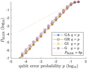
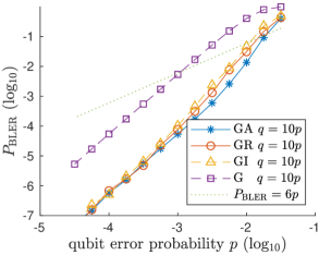
Figure 1: Phenomenological noise model (A) with depolarizing errors (probability $p$) and syndrome bit measurement error probability $q=p$ (left) and $q=10p$ (right). Symbols show the block error probability $P_{\rm BLER}$ for four decoders as indicated, see text for details. Dotted lines give the nominal single-qubit break-even threshold, $P_{\rm BLER}=p$.

In simulations with phenomenological error model (B) we measured the average fail time of the code[10]. Namely, in each simulation round $j$ repeated decoding cycles are done until decoding failure after round $t_{j}$; the corresponding average after $N\geq 100$ simulation rounds was recorded. Effective block error rate $P_{\rm BLER}=1/(\bar{t}-1)$ was then extracted from the average fail time $\bar{t}$ assuming Poisson distribution of life times $t_{j}^{\prime}=t_{j}-1$ with parameter $\lambda=P_{\rm BLER}$. We decoded every cycle $t$ separately, using the accumulated data error $\hat{{\bf e}}_{1}+\hat{{\bf e}}_{2}+\ldots+\hat{{\bf e}}_{t-1}$ found in the previous cycles as an offset. Consistent with the standard protocol for quantum LDPC codes[10], a failure would be recorded if at time step $t$ decoding with zero syndrome error $\boldsymbol{\epsilon}_{t}={\bf 0}$ gives a logical error. Otherwise, a new estimated error $\hat{{\bf e}}_{t}$ would be computed with the syndrome error $\boldsymbol{\epsilon}_{t}$ present, and calculation repeated at $t=t+1$. The results are shown in Fig. 2; they are largely consistent with those for phenomenological error model (A).

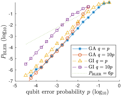
Figure 2: Effective block error rate $P_{\rm BLER}$ with phenomenological error model B. Only results for GA and single-interval GI decoders as indicated are shown.

In simulations with circuit error model (C) we constructed the actual circuits for measuring quantum operators corresponding to rows of ${\bf G}$, including the redundant rows for code GA, with the attempt to maximally parallelize the measurements. We then used a separate program to generate random Pauli errors with probability $p_{1}$ per interval between the gates, propagated the errors through the circuit, and recorded the actual accumulated error $\underline{{\bf e}}_{t}$ and the measured syndrome ${\bf s}_{t}$ at the end of each measurement cycle $t=1,2,\ldots$. Additional syndrome measurement error $q_{1}$ was added at the time of subsequent processing. These data then have been used with the decoders identical to those for model B.

The obtained effective block error rates are plotted in Fig. 3. One striking difference with phenomenological error models A and B is that the calculated curves no longer have quadratic dependence on BER, as would be expected for a code with distance $d=3$. The reason is that we have used non-FT circuits in simulations. As a result, e.g., a single ancilla error can propagate and multiply through the circuit, resulting in a higher-weight error which cannot be corrected by the code.

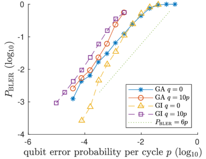
Figure 3: Effective block error rate (per gate) for phenomenological error model C as a function of gate error probability $p_{1}$ scaled by cycle duration.

VII Discussion and Future Work

In conclusion, in this work we introduced quantum convolutional data-syndrome codes, constructed an efficient decoder for this class of codes, and analyzed numerically the performance of a family of DS codes based on a single QCC with parameters $[[24,6,3]]$ using three distinct error models. In particular, this was the first time a DS code has been simulated with the circuit error model.

Here we exclusively relied on the QCCs designed in Ref. [12]. These codes have relatively high weights of stabilizer generators. It is an open question whether degenerate QCCs exist, with small-weight generators, large distances, and trellises with reasonably small memory sizes. For the purpose of constructing convolutional DS codes, one would further like to have a QCC with a redundant set of minimum-weight stabilizer generators. For such codes, degenerate Viterbi decoding algorithm[19] would be particularly useful.

Our limited simulation results indicate that a DS code with large-distance classical syndrome code may show competitive performance in the regime where measurement errors are significant, even though the corresponding generators may have larger weights. This regime is experimentally relevant, e.g., for superconducting transmon qubits with dispersive readout, where measurement time can be as large as 500ns, compared to under 50ns two-qubit gates, with the error probabilities scaling accordingly. It is an open question whether similarly constructed non-convolutional DS codes could be useful in this regime, e.g., for optimizing the performance of surface codes in the current or near-future generation of quantum computers.

One obvious way to improve the practical performance of DS codes is by using FT gadgets for generator measurements, to control error propagation. In particular, we intend to try flag measurement circuits[20], as this technique has relatively small overhead in the number of qubits.

References

- [1] E. Dennis, A. Kitaev, A. Landahl, and J. Preskill, “Topological quantum memory,” J. Math. Phys., vol. 43, p. 4452, 2002.
- [2] H. Bombin, R. W. Chhajlany, M. Horodecki, and M. A. Martin-Delgado, “Self-correcting quantum computers,” New J. of Physics, vol. 15, p. 055023, 2013.
- [3] K. Duivenvoorden, N. P. Breuckmann, and B. M. Terhal, “Renormalization group decoder for a four-dimensional toric code,” unpublished, arXiv:1708.09286.
- [4] Y. Fujiwara, “Ability of stabilizer quantum error correction to protect itself from its own imperfection,” Phys. Rev. A, vol. 90, p. 062304, Dec 2014.
- [5] A. Ashikhmin, C. Y. Lai, and T. A. Brun, “Robust quantum error syndrome extraction by classical coding,” in 2014 IEEE International Symposium on Information Theory, 2014, pp. 546–550.
- [6] ——, “Correction of data and syndrome errors by stabilizer codes,” in 2016 IEEE Int. Symp. Inf. Th. (ISIT), 2016, pp. 2274–2278.
- [7] H. Bombín, “Single-shot fault-tolerant quantum error correction,” Phys. Rev. X, vol. 5, p. 031043, Sep 2015.
- [8] B. J. Brown, N. H. Nickerson, and D. E. Browne, “Fault-tolerant error correction with the gauge color code,” Nature Commun., vol. 7, p. 12302, 2016.
- [9] E. T. Campbell, “A theory of single-shot error correction for adversarial noise,” 2018, to be published in Quant. Science and Techn. (2019).
- [10] D. S. Wang, A. G. Fowler, and L. C. L. Hollenberg, “Surface code quantum computing with error rates over ,” Phys. Rev. A, vol. 83, p. 020302, Feb 2011.
- [11] A. J. Landahl, J. T. Anderson, and P. R. Rice, “Fault-tolerant quantum computing with color codes,” 2011, presented at QIP 2012, Dec. 12–16.
- [12] G. D. Forney, M. Grassl, and S. Guha, “Convolutional and tail-biting quantum error-correcting codes,” IEEE Trans. Inf. Th., vol. 53, pp. 865–880, 2007.
- [13] A. J. Viterbi, “Error bounds for convolutional codes and an asymptotically optimum decoding algorithm,” IEEE Trans. Inf. Th., vol. 13, pp. 260–269, 1967.
- [14] R. Johannesson and K. S. Zigangirov, Fundamentals of convolutional coding. John Wiley & Sons, 2015, vol. 15.
- [15] A. R. Calderbank, E. M. Rains, P. M. Shor, and N. J. A. Sloane, “Quantum error correction via codes over GF(4),” IEEE Trans. Info. Theory, vol. 44, pp. 1369–1387, 1998.
- [16] P. W. Shor, “Fault-tolerant quantum computation,” in Proc. 37th Ann. Symp. on Fundamentals of Comp. Sci., IEEE. Los Alamitos: IEEE Comp. Soc. Press, 1996, pp. 56–65; A. M. Steane, “Active stabilization, quantum computation, and quantum state synthesis,” Phys. Rev. Lett., vol. 78, pp. 2252–2255, Mar 1997; D. Gottesman, “Theory of fault-tolerant quantum computation,” Phys. Rev. A, vol. 57, pp. 127–137, Jan 1998.
- [17] D. Gottesman, “The Heisenberg representation of quantum computers,” in Group22: Proceedings of the XXII International Colloquium on Group Theoretical Methods in Physics, S. P. Corney, R. Delbourgo, and P. D. Jarvis, Eds. Cambridge, MA: International Press, 1998, pp. 32–43.
- [18] V. Sidorenko and V. Zyablov, “Decoding of convolutional codes using a syndrome trellis,” IEEE Trans. Inf. Th., vol. 40, pp. 1663–1666, 1994.
- [19] E. Pelchat and D. Poulin, “Degenerate Viterbi decoding,” IEEE Trans. Inf. Th., vol. 59, pp. 3915–3921, 2013.
- [20] C. Chamberland and M. E. Beverland, “Flag fault-tolerant error correction with arbitrary distance codes,” 2017, unpublished, arXiv:1708.02246.