Neural Video Compression using Spatio-temporal Priors

Abstract

The pursuit of higher compression efficiency continuously drives the advances of video coding technologies. Fundamentally, we wish to find better “predictions” or “priors” that are reconstructed previously to remove the signal dependency efficiently and to accurately model the signal distribution for entropy coding. In this work, we propose a neural video compression framework, leveraging the spatial and temporal priors, independently and jointly to exploit the correlations in intra texture, optical flow based temporal motion and residuals. Spatial priors are generated using downscaled low-resolution features, while temporal priors (from previous reference frames and residuals) are captured using a convolutional neural network based long-short term memory (ConvLSTM) structure in a temporal recurrent fashion. All of these parts are connected and trained jointly towards the optimal rate-distortion performance. Compared with the High-Efficiency Video Coding (HEVC) Main Profile (MP), our method has demonstrated averaged 38% Bjontegaard-Delta Rate (BD-Rate) improvement using standard common test sequences, where the distortion is multi-scale structural similarity (MS-SSIM).

Index Terms—  Spatial prior, temporal prior, optical flow, deep learning, neural video compression

1 Introduction

Over the past three decades, successful video compression technologies have been following the similar hybrid block-based transform and motion-compensation framework with handcrafted coding tools, such as recursive block-size, directional intra prediction, discrete cosine transform (DCT), interpolation, context-adaptive entropy coding, etc, resulting in several well-known international standards, e.g., HEVC [1] and emerging versatile video coding (VVC) [2]. All of these and other technical explorations in video compression are trying to exploit and remove signal redundancy using “causal priors”, e.g, reconstructed neighbor pixels, previous frames, context probability of neighbors, in video content, spatially, temporally and statistically [3], for better compact representation at the same quality.

Motivated by the recent advances in deep learning, a variety of deep neural network (DNN) based image/video compression methods were developed via end-to-end learned (not handcrafted) coding tools [4, 5, 6, 7, 8, 9, 10]. Either conventional or recent emerging learning based video compressions are primarily trying to exploit the correlations between existing priors and “pixels-to-be-coded”. In addition to previously reconstructed pixels and context probabilities used in traditional video coding methods, DNN solutions could also generate hyperpriors in feature domain for better prediction.

In this work, we have presented a neural video compression (NVC) framework in Fig. 1, leveraging the end-to-end learning to generate latent features for compact representation of spatial intra texture, temporal motion and statistical context probability. Joint spatio-temporal priors have been used extensively to improve the compression efficiency, for example, 1) spatial priors for both conditional probability modeling and reconstruction of intra texture (cf. Fig. 1); 2) temporal priors for frame reconstruction (cf. Fig. 1); and 3) joint spatio-temporal priors for temporal predictive residual encoding (cf. Fig. 1) (e.g., context probability) and reconstruction.

Spatial priors are generated using the low-resolution (e.g., via aggregated downscaling) representations from the same image content, while temporal priors are provided using the ConvLSTM [11, 12] to capture the long-short dependency of previously processed frames. Temporal motion representation often plays an important role for video compression. Traditional methods adopt straightforward but effective variable block size based motion estimation to exploit the temporal correlations. But, in this work, we have turned to more fundamental optical flow for motion description instead.

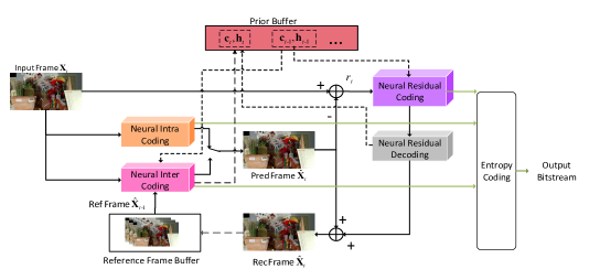
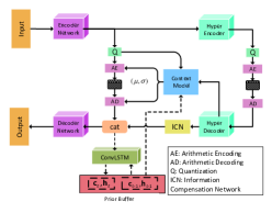
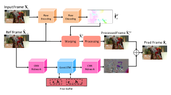
Fig. 1: Neural video compression framework: (a) overall architecture with neural intra, inter and residual coding; (b) intra and residual coding; (c) inter coding with flow processing and temporal recurrent update.

We have evaluated our NVC for a low-delay, e.g., IPPP, coding structure, where except the first frame is encoded as an intra frame, all the rest frames are inter-coded with unidirectional forward prediction. Performance comparisons have been carried out with well-known H.264/AVC High Profile (HP) [13] and HEVC MP [1], using industry leading x264 (https://git.videolan.org/git/x264.git) and x265 (http://x265.org/). For fairness, both x264 and x265 are constrained with IPPP low-delay encoding configuration with the other parameters remained as default. Among those standard common test video sequences, our NVC has demonstrated superior coding efficiency over both H.264/AVC HP and HEVC MP, e.g., $\approx$38% BD-Rate [14] improvements against the HEVC MP. Note that distortion measurement used in evaluation is the MS-SSIM [15] presented in decibel (dB) scale.

2 Neural Video Compression: From Model-Driven to Data-Driven Solution

Our NVC has attempted to define a way for efficient video compression through data-driven learning, rather than the traditional model-driven coding tool (e.g., transform model, motion model, etc) development. Details will be unfolded in subsequent paragraphs.

2.1 Neural Intra Coding

Neural intra (texture) coding has tried to exploit the correlation within current video frame. As shown in Fig. 1, we utilize a variational autoencoder with embedded hyperpriors for high-efficiency image coding. Similar architecture is also used in [4]. We use deep residual learning (ResNet) [16] with generalized divisive normalization (GDN) transform based activation, but not conventional rectified linear unit (ReLU), for fast convergence in training and more compact latent features, in both encoder network $\mathbb{E}$ and decoder network $\mathbb{D}$. Convolution with parametric ReLU is used for hyper encoder and decoder. Quantization $Q$ is approximated by adding uniform noise in training, but carried out with ROUND($\cdot$) operation in inference.

An accurate probability distribution model of quantized features is the key for high-efficiency compression, not only for the arithmetic encoding (AE), but also for the rate estimation of rate-distortion optimization [17] and bit allocation. We jointly leverage the autoregressive information (i.e., distribution of quantized features) and hyperpriors (i.e., distribution of decoded hyper-features) for conditional context probability $P$ modeling with accurate mean ($\mu$) and variance ($\sigma$) prediction assuming a Gaussian distributed probability mass function, i.e.,

$$(\mu,\sigma)={\prod_{i}}p\left(\hat{x}_{i}|\hat{x}_{1},...,\hat{x}_{i-1},{\hat{\bf z}_{t}}\right).$$ (1)

Here, $\hat{x}_{1},{\hat{x}}_{2},...,\hat{x}_{i-1}$ denote the causal (and possibly reconstructed) pixels prior to current pixel $\hat{x}_{i}$ and $\hat{\bf z}_{t}$ are the hyperpriors, for image $\hat{\bf X}_{t}$. Probability of each pixel symbol can be simply derived using

$$p_{\hat{x}|\hat{x}_{1},...,\hat{x}_{i-1},\hat{\bf z}_{t}} (\hat{x}|\hat{x}_{1},...,\hat{x}_{i-1},\hat{\bf z}_{t})$$

$$\mbox{~{}~{}~{}~{}}={\prod_{i}}(\mathcal{N(\mu,\sigma)}*\mathcal{U}(-\frac{1}{2},\frac{1}{2}))(\hat{x}_{i}).$$ (2)

In addition to use hyperpriors $\hat{\bf z}_{t}$ for conditional probability improvement, we have developed an Information Compensation Network (ICN) to fuse and concatenate (cat operation in Fig. 1) decoded hyperpriors with latent features for better reconstruction.

2.2 Neural Inter Coding

The key issues for improving the efficiency of temporal inter coding are two folds. One is to accurately represent the motion between consecutive frames, and the other is to have high-fidelity reconstructions for compensation.

First, we use optical flow $f_{t}$ for accurate motion representation that are learned between consecutive frames, e.g., ${\bf X}_{t}$ and $\hat{\bf X}_{t-1}$, as shown in Fig. 1. A compressed flow representation $\hat{f}_{t}$ is encoded into the bitstream for delivery. For compensation, $\hat{f}_{t}$ is then decoded into $\hat{f}^{d}_{t}$ for warping with reference frame to have ${\bf X}^{w}_{t}$, i.e.,

$$\hat{f}^{d}_{t} ={\mathbb{F}}_{d}\left({\mathbb{F}}_{e}\left(\hat{\bf X}_{t-1},{\bf X}_{t}\right)\right),$$ (3)

$${\hat{\bf X}}^{w}_{t} ={\bf warp}\left(\hat{\bf X}_{t-1},\hat{f}^{d}_{t}\right).$$ (4)

Here ${\mathbb{F}}_{e}$ and ${\mathbb{F}}_{d}$ represent the cascaded optical flow encoder and decoder network [18]. To avoid quantization induced motion noise, our flow network is first pre-trained with uncompressed frames ${\bf X}_{t-1}$ and ${\bf X}_{t}$. Then we replace the former one ${\bf X}_{t-1}$ using the decoded reference frame ${\hat{\bf X}}_{t-1}$ as described in Eq. (3) and (4). Note that we have directly utilized the decoded flow $\hat{f}^{d}_{t}$ for end-to-end training.

Oftentimes, warped frame ${\hat{\bf X}}^{w}_{t}$ suffers from poor quality due to noisy flow estimation, unexpected object occlusion, etc. To improve the quality of warped frames, we propose to apply a processing network using ten residual blocks with embedded re-sampling to enlarge the receptive field, resulting in ${\hat{\bf X}}^{wp}_{t}$. Such methods have been used in denoising and deblurring applications to improve the quality of reconstruction.

Even with processing network included, we have observed that high frequency components are generally missing in ${\hat{\bf X}}^{wp}_{t}$. Motivated by [19] that uses learned multi-frame residual information to improve the super resolution quality, we have attempted to apply the temporal recurrent network that is based on the ConvLSTM to capture and augment the high frequency priors to derive the $\tilde{\bf X}_{t}$ for temporal prediction, i.e.,

$$({\bf c}_{t},{\bf h}_{t})={\rm ConvLSTM}({\bf\Delta}_{t},{\bf c}_{t-1},{\bf h}_{t-1}),$$ (5)

where ${\bf c}_{t},{\bf h}_{t}$ is updated state at $t$ slot with ${\bf c}_{t-1}$ used as a memory gate, and ${\bf h}_{t-1}$ as aggregated prior (i.e., probability, high frequency component, etc) update. ${\bf\Delta}_{t}$ is generally referred as the input feature vector. Here it is extracted features from reference frame $\hat{\bf X}_{t-1}$ in Fig. 1.

(a) KristenAndSara 1080p

(b) vidyo1 720p

(c) BasketBallDrive 1080p

(d) vidyo3 720p

(e) Cactus 1080p

(f) FourPeople 720p

Fig. 2: Illustration of the rate-distortion performance for six different sequences. Here we use $-10\log_{10}(1-d)$ to represent raw MS-SSIM ($d$) in dB scale.

2.3 Neural Residual Coding

Temporal residual coding shares the similar architecture as the intra coding shown in Fig. 1, but with an augmented ConvLSTM to capture the aggregated temporal priors $\hat{\bf h}_{t}$ additionally for residual probability model improvement. Here, ${\bf\Delta}_{t}$ in Eq. (5) refers to the concatenated features in current frame $\hat{\bf Y}_{t}={\bf CAT}(\hat{\bf X}_{t},\rm{ICN}(\hat{\bf z}_{t}))$ in Fig. 1.

We assume the same Gaussian distribution for residuals. Thus, Eq. (1) can be rewritten as

$$(\mu_{r},\sigma_{r})={\prod_{i}}p(\hat{r}_{i}|\hat{r}_{1},...,\hat{r}_{i-1},\hat{\bf z}_{t},{\bf h}_{t-1}),$$ (6)

with aggregated temporal priors for residual probability modeling. $\hat{r}_{i},i=0,1,2,...$ are pixels of residual frame $\hat{\bf r}_{t}$. We then can simply use the cumulative distribution function (CDF) to calculate the probability of each pixel:

$$p_{\hat{r}|(\hat{r}_{1},...,\hat{r}_{i-1},\hat{\bf z}_{t},{\bf h}_{t-1})}(\hat{r}|\hat{r}_{1},...,\hat{r}_{i-1},\hat{\bf z}_{t},{\bf h}_{t-1})$$

$$\mbox{~{}~{}~{}~{}}={\prod_{i}}(\mathcal{N}{(\mu_{r},\sigma_{r})}*\mathcal{U}(-\frac{1}{2},\frac{1}{2}))(\hat{r}_{i}).$$ (7)

3 End-to-End Training Strategy

It is difficult to train multiple networks jointly on-the-fly for our NVC. Thus, we pre-train the intra coding and flow coding networks first, followed by the jointly training with pre-trained nets for an overall rate-distortion optimization [17], i.e.,

$$L={\frac{\lambda_{1}}{n}{\sum_{t=0}^{n}}{\mathbb{D}}_{1}(\hat{{\bf X}}_{t},{{\bf X}_{t}})} +{\frac{\lambda_{2}}{n}{\sum_{t=0}^{n}}{\mathbb{D}}_{2}(\hat{\bf X}_{t}^{wp},{{\bf X}_{t}})}$$

$$+R_{s}+{\frac{1}{n-1}{\sum_{t=1}^{n}}R_{t}},$$ (8)

where ${\mathbb{D}}_{1}$ is measured using MS-SSIM, and ${\mathbb{D}}_{2}$ is the warp loss evaluated using $L$1 norm and total variation loss. $R_{s}$ represents the bit rate of intra frame and $R_{t}$ is the bit rate of inter frames including bits for residual and flow. Currently, $\lambda_{1}$ and $\lambda_{2}$ will be adapted according to the specified overall bit rate and bit consumption percentage of flow information in inter coding.

Table 1: BD-Rate Gain of our NVC versus HEVC MP

Sequence	Resolution	FPS	BD-Rate Gain
KristenAndSara	1920x1080	60	-96.96%
vidyo1	1280x720	60	-54.32%
BasketBallDrive	1920x1080	50	-12.07%
vidyo3	1280x720	60	-49.15%
Cactus	1920x1080	50	-2.27%
FourPeople	1280x720	60	-13.92%
Ave.			-38.12%

We start at a learning rate (LR) of $10^{-4}$ and reduce it by half every 30 epochs. We choose vimeo dataset [20] and randomly crop the data into 192$\times$192 spatially, as our training set. To well balance the efficiency of temporal information learning and training memory consumption, we have enrolled 5 frames to train the video compression framework and shared the weights for the rest in the time domain.

4 Experimental Studies

We have evaluated our NVC framework using BD-Rate but with distortion measured using MS-SSIM in dB scale. All simulation candidates, i.e., NVC, H.264/AVC HP, HEVC MP, use IPPP mode to encode the video data with the same GOP of 8 for fair comparison. Well recognized x264 and x265 softwares are used for H.264/AVC HP and HEVC MP, respectively. Several standard test sequences in different content classes are tested, and results have shown that our NVC presents a noticeable BD-Rate improvement compared with traditional H.264/AVC HP and HEVC MP as shown in Fig. 2. In the meantime, BD-Rate reduction compared with HEVC MP is calculated and shown in Table 1, where $\approx$ 38.12% BD-Rate gain is reported on average.

We have also provided snapshots for original raw, NVC, H.264/AVC HP and HEVC MP encoded frames, respectively in Fig. 3. At the similar quality with MS-SSIM close to 0.988, our NVC has demonstrated significant bit rate reduction compared with the H.264/AVC HP and HEVC MP.

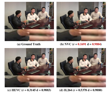
Fig. 3: Snapshots of performance evaluation at the same quality ($r$ for bit rate at bits per pixel, and $d$ for MS-SSIM).

5 Conclusion

We proposed a neural video compression framework leveraging the spatio-temporal priors jointly, which outperforms the well-known H.264/AVC and HEVC with noticeable BD-Rate gains (i.e., 38% on average), resulting in the state-of-the-art coding performance. Spatial priors are derived from the downscaled image representations and temporal priors are captured using a recurrent network. As for future studies, bidirectional temporal prediction is one of the primary focuses to further improve the compression efficiency. In the meantime, adaptive bit rate allocation among intra texture, flow motion and residual with optimal rate-distortion efficiency will be another exploration avenue.

References

- [1] G. J. Sullivan, J. Ohm, W. Han, and T. Wiegand, “Overview of the high efficiency video coding (hevc) standard,” IEEE Transactions on Circuits and Systems for Video Technology, vol. 22, no. 12, pp. 1649–1668, Dec 2012.
- [2] B. Bross, J. Chen, and S. Liu, “Versatile video coding (draft 3),” Doc. JVET L1001, Oct. 2018.
- [3] G. J. Sullivan and T. Wiegand, “Video compression - from concepts to the h.264/avc standard,” Proceedings of the IEEE, vol. 93, no. 1, pp. 18–31, Jan 2005.
- [4] Johannes Ballé, David Minnen, Saurabh Singh, Sung Jin Hwang, and Nick Johnston, “Variational image compression with a scale hyperprior,” arXiv preprint arXiv:1802.01436, 2018.
- [5] Haojie Liu, Tong Chen, Qiu Shen, Tao Yue, and Zhan Ma, “Deep image compression via end-to-end learning,” in The IEEE Conference on Computer Vision and Pattern Recognition (CVPR) Workshops, June 2018.
- [6] Oren Rippel and Lubomir Bourdev, “Real-time adaptive image compression,” arXiv preprint arXiv:1705.05823, 2017.
- [7] Fabian Mentzer, Eirikur Agustsson, Michael Tschannen, Radu Timofte, and Luc Van Gool, “Conditional probability models for deep image compression,” in IEEE Conference on Computer Vision and Pattern Recognition (CVPR), 2018, vol. 1, p. 3.
- [8] Tong Chen, Haojie Liu, Qiu Shen, Tao Yue, Xun Cao, and Zhan Ma, “Deepcoder: A deep neural network based video compression,” in Visual Communications and Image Processing (VCIP), 2017 IEEE. IEEE, 2017, pp. 1–4.
- [9] Guo Lu, Wanli Ouyang, Dong Xu, Xiaoyun Zhang, Chunlei Cai, and Zhiyong Gao, “Dvc: An end-to-end deep video compression framework,” arXiv preprint arXiv:1812.00101, 2018.
- [10] Oren Rippel, Sanjay Nair, Carissa Lew, Steve Branson, Alexander G Anderson, and Lubomir Bourdev, “Learned video compression,” arXiv preprint arXiv:1811.06981, 2018.
- [11] Felix Gers, Long short-term memory in recurrent neural networks, Ph.D. thesis, Verlag nicht ermittelbar, 2001.
- [12] SHI Xingjian, Zhourong Chen, Hao Wang, Dit-Yan Yeung, Wai-Kin Wong, and Wang-chun Woo, “Convolutional lstm network: A machine learning approach for precipitation nowcasting,” in Advances in neural information processing systems, 2015, pp. 802–810.
- [13] T. Wiegand, G. J. Sullivan, G. Bjontegaard, and A. Luthra, “Overview of the h.264/avc video coding standard,” IEEE Transactions on Circuits and Systems for Video Technology, vol. 13, no. 7, pp. 560–576, July 2003.
- [14] Gisle Bjontegaard, “Calculation of average psnr differences between rd-curves,” VCEG-M33, 2001.
- [15] Zhou Wang, Eero P Simoncelli, and Alan C Bovik, “Multiscale structural similarity for image quality assessment,” in The Thrity-Seventh Asilomar Conference on Signals, Systems & Computers, 2003. Ieee, 2003, vol. 2, pp. 1398–1402.
- [16] Kaiming He, Xiangyu Zhang, Shaoqing Ren, and Jian Sun, “Deep residual learning for image recognition,” in Proceedings of the IEEE conference on computer vision and pattern recognition, 2016, pp. 770–778.
- [17] G. J. Sullivan and T. Wiegand, “Rate-distortion optimization for video compression,” IEEE Signal Processing Magazine, vol. 15, no. 6, pp. 74–90, Nov 1998.
- [18] Eddy Ilg, Nikolaus Mayer, Tonmoy Saikia, Margret Keuper, Alexey Dosovitskiy, and Thomas Brox, “Flownet 2.0: Evolution of optical flow estimation with deep networks,” in 2017 IEEE conference on computer vision and pattern recognition (CVPR). IEEE, 2017, pp. 1647–1655.
- [19] Younghyun Jo, Seoung Wug Oh, Jaeyeon Kang, and Seon Joo Kim, “Deep video super-resolution network using dynamic upsampling filters without explicit motion compensation,” in Proceedings of the IEEE Conference on Computer Vision and Pattern Recognition, 2018, pp. 3224–3232.
- [20] Tianfan Xue, Baian Chen, Jiajun Wu, Donglai Wei, and William T Freeman, “Video enhancement with task-oriented flow,” arXiv preprint arXiv:1711.09078, 2017.