Eulerian orientations and the six-vertex model
on planar maps

Abstract.

We address the enumeration of planar 4-valent maps equipped with an Eulerian orientation by two different methods, and compare the solutions we thus obtain. With the first method we enumerate these orientations as well as a restricted class which we show to be in bijection with general Eulerian orientations. The second method, based on the work of Kostov, allows us to enumerate these 4-valent orientations with a weight on some vertices, corresponding to the six vertex model. We prove that this result generalises both results obtained using the first method, although the equivalence is not immediately clear.

1. Introduction

In 2000, Zinn-Justin [ZJ00] and Kostov [Kos00] studied the six-vertex model on a random lattice. In combinatorial terms, this means counting rooted 4-valent (or: quartic) planar maps equipped with an Eulerian orientation of the edges: that is, every vertex has equal in- and out-degree (Figs. 1 and 3). Every vertex is weighted $t$, and every alternating vertex gets an additional weight $\gamma$, yielding a generating function ${\sf Q}(t,\gamma)$:

$$Q(t,\gamma)=\left(2\,\gamma+2\right)t+\left(9\,{\gamma}^{2}+16\,\gamma+10\right){t}^{2}+\left(54\,{\gamma}^{3}+132\,{\gamma}^{2}+150\,\gamma+66\right){t}^{3}+O({t}^{4}).$$

For instance, the 4 orientations accounting for the coefficient of $t$ are the following ones (the edge carrying a double arrow is the root edge, oriented canonically):

Kostov solved this problem exactly, but the form of his solution is quite complicated and its derivation is not entirely rigourous.

Figure 1. The two types of vertices in the six-vertex model.

Recently Bonichon, Bouquet-Mélou, Dorbec and Pennarun [BBMDP17] posed the analogous problem of enumerating Eulerian orientations of general planar maps by edges (where the vertex degree is not restricted). They were followed by Elvey Price and Guttmann who wrote an intricate system of functional equations defining the associated generating function [EPG18]. This allowed them to compute the number $g_{n}$ of Eulerian orientations with $n$ edges for large values of $n$, and led them to a conjecture on the asymptotic behaviour of $g_{n}$. In a similar way they conjectured the asymptotic behaviour of the coefficients $q_{n}$ of ${\sf Q}(t,1)$, counting Eulerian orientations of quartic maps, though this prediction had already been in the physics papers [Kos00, ZJ00]. The conjectured asymptotic forms of the sequences $(q_{n})_{n\geq 0}$ and $(g_{n})_{n\geq 0}$ led us to conjecture exact forms of the two sequences. These are the conjectures that we prove in the following two theorems.

Theorem 1.

Let ${\sf R}(t)\equiv{\sf R}$ be the unique formal power series with constant term $0$ satisfying

(1) $$t=\sum_{n\geq 0}\frac{1}{n+1}{2n\choose n}^{2}{\sf R}^{n+1}.$$

Then the generating function of rooted planar Eulerian orientations, counted by edges, is

$${\sf G}(t)=\frac{1}{2}{\sf Q}(t,0)=\frac{1}{4t^{2}}\left(t-2t^{2}-{\sf R}(t)\right)=t+5t^{2}+33t^{3}+\cdots.$$

Theorem 2.

Let ${\sf R}(t)\equiv{\sf R}$ be the unique formal power series with constant term $0$ satisfying

$$t=\sum_{n\geq 0}\frac{1}{n+1}{2n\choose n}{3n\choose n}{\sf R}^{n+1}.$$

Then the generating function of quartic rooted planar Eulerian orientations, counted by vertices, is

$${\sf Q}(t,1)=\frac{1}{3t^{2}}\left(t-3t^{2}-{\sf R}(t)\right)=4t+35t^{2}+402t^{3}+\cdots.$$

The first step in our proof of Theorem 1 is a bijection that relates general Eulerian orientations to quartic ones having no alternating vertex (Section 2). It implies that ${\sf G}(t)=\frac{1}{2}{\sf Q}(t,0)$. We then characterise the generating functions ${\sf Q}(t,0)$ and ${\sf Q}(t,1)$ by a system of functional equations using some new decompositions of planar maps. We then solve these equations exactly (Section 3). Details on this approach as well as basic definitions on planar maps can be found in [BMEP].

In Section 4 we use a different method to analyse the generating function ${\sf Q}(t,\gamma)$ for general $\gamma$, following Kostov’s solution to the six-vertex model. We re-derive the first part of his study, which yields a system of functional equations characterising ${\sf Q}(t,\gamma)$, using a combinatorial argument. We then follow Kostov’s solution to these equations and fix a mistake, which gives us a parametric expression of ${\sf Q}(t,\gamma)$ in terms of the Jacobi theta function

$$\vartheta(z,q)=2\sin(z)q^{1/8}\prod_{n=1}^{\infty}(1-2\cos(2z)q^{n}+q^{2n})(1-q^{n}).$$

Theorem 3.

Write $\gamma=-2\cos(2\alpha)$, and let $q(t,\gamma)\equiv q=t+\left(6\,\gamma+6\right){t}^{2}+\cdots$ be the unique formal power series in $t$ with constant term $0$ satisfying

$$t=\frac{\cos\alpha}{64\sin^{3}\alpha}\left(-\frac{\vartheta(\alpha,q)\vartheta^{\prime\prime\prime}(\alpha,q)}{\vartheta^{\prime}(\alpha,q)^{2}}+\frac{\vartheta^{\prime\prime}(\alpha,q)}{\vartheta^{\prime}(\alpha,q)}\right),$$

where all derivatives are with respect to the first variable. Moreover, define the series ${\sf R}(t,\gamma)$ by

$${\sf R}(t,\gamma)=\frac{\cos^{2}\alpha}{96\sin^{4}\alpha}\frac{\vartheta(\alpha,q)^{2}}{\vartheta^{\prime}(\alpha,q)^{2}}\left(-\frac{\vartheta^{\prime\prime\prime}(\alpha,q)}{\vartheta^{\prime}(\alpha,q)}+\frac{\vartheta^{\prime\prime\prime}(0,q)}{\vartheta^{\prime}(0,q)}\right).$$

Then the generating function of quartic rooted planar Eulerian orientations, counted by vertices, with a weight $\gamma$ per alternating vertex is

$${\sf Q}(t,\gamma)=\frac{1}{(\gamma+2)t^{2}}\left(t-(\gamma+2)t^{2}-{\sf R}(t,\gamma)\right).$$

It is not clear why, in the two special cases $\gamma=0,1$, this theorem is equivalent to Theorems 1 and 2 respectively. We prove this equivalence in Section 5. We conclude with a discussion on further projects.

Figure 2. A rooted Eulerian orientation (solid edges; the root edge is shown with a double arrow, and its orientation is chosen canonically) and the corresponding dual labelled map (dashed edges). The labelling rule is shown on the right.

2. Bijection for general Eulerian orientations

The first step in the enumeration of Eulerian orientations is a simple bijection, introduced in [EPG18], to certain labelled maps.

Definition 4.

A labelled map is a rooted planar map with integer labels on its vertices, such that adjacent labels differ by $1$ and the root edge is labelled from $0$ to $1$.

The bijection is illustrated in Figure 2. The idea is that an Eulerian orientation of edges of a map determines a height function on the vertices of its dual. A restriction of this bijection shows that quartic Eulerian orientations are in bijection with labelled quadrangulations (every face has degree 4).

For the next step, we use a bijection of Miermont, Ambjørn and Budd [Mie09, AB13] to show that labelled maps having $n$ edges are in 1-to-2 correspondence with colourful labelled quadrangulations having $n$ faces. By colourful we mean that each face has three distinct labels, or equivalently, that the corresponding quartic orientation has no alternating vertex. This bijection generalizes a bijection of [CS04], and is illustrated in Figure 3. It implies that ${\sf G}(t)=\frac{1}{2}{\sf Q}(t,0)$.

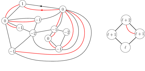
Figure 3. A labelled quadrangulation $Q$ (black edges) and the corresponding labelled map $L$ (red edges). The rule for drawing red edges is shown on the right. Note that the two local minima of $Q$, both labelled $-2$, disappear in the construction.

In fact, this pair of bijections allows us to understand the more general series ${\sf Q}(t,\gamma)$ as a generalisation of ${\sf G}(t)$ in terms of Eulerian partial orientations. These are planar maps in which some edges are oriented, in such a way that each vertex has equal in- and out-degree.

Proposition 5.

The series ${\sf Q}(t,\gamma)$ counting rooted quartic Eulerian orientations also counts rooted Eulerian partial orientations with a weight $t$ per edge and an additional weight $\gamma$ per undirected edge (the root edge may be undirected or directed in either direction).

Here are the 4 partial orientations that account for the coefficient $2+2\gamma$ of $t$ in ${\sf Q}(t,\gamma)$:

3. The number of planar Eulerian orientations

In this section we give a very brief summary of our solutions to the cases ${\sf Q}(t,0)$ and ${\sf Q}(t,1)$. The full details are in [BMEP]. We define three classes $\mathcal{P},\mathcal{D}$ and $\mathcal{C}$ of labelled quadrangulations and decompose them recursively, using in particular a new contraction operation. We thus characterise the series ${\sf Q}(t,0)=2{\sf G}(t)$ as follows.

Proposition 6.

There is a unique $3$-tuple of series, denoted ${\sf P}(t,y)$, ${\sf C}(t,x,y)$ and ${\sf D}(t,x,y)$, belonging respectively to $\mathbb{Q}[[y,t]]$, $\mathbb{Q}[x][[y,t]]$ and $\mathbb{Q}[[x,y,t]]$, and satisfying the following equations:

$${\sf P}(t,y) =\frac{1}{y}[x^{1}]{\sf C}(t,x,y),$$

$${\sf D}(t,x,y) =\frac{1}{1-{\sf C}\left(t,\frac{1}{1-x},y\right)},$$

$${\sf C}(t,x,y) =xy[x^{\geq 0}]\left({\sf P}(t,tx){\sf D}\left(t,\frac{1}{x},y\right)\right),$$

together with the initial condition ${\sf P}(t,0)=1$ (the operator $[x^{\geq 0}]$ extracts all monomials in which the exponent of $x$ is non-negative).

The generating function ${\sf Q}(t,0)$ is related to these series by the equation

$${\sf Q}(t,0)=[y^{1}]{\sf P}(t,y)-1.$$

We then solve this system of equations as follows, writing ${\sf P}$, ${\sf C}$ and ${\sf D}$ in terms of the series ${\sf R}(t)$ defined in Theorem 1:

$$t{\sf P}(t,ty)=\sum_{n\geq 0}\sum_{j=0}^{n}\frac{1}{n+1}{2n\choose n}{2n-j\choose n}y^{j}{\sf R}^{n+1},$$

$${\sf C}(t,x,ty)=1-\exp\left(-\sum_{n\geq 0}\sum_{j=0}^{n}\sum_{i=0}^{n}\frac{1}{n+1}{2n-i\choose n}{2n-{j}\choose n}x^{i+1}y^{j+1}{\sf R}^{n+1}\right),$$

$${\sf D}(t,x,ty)=\exp\left(\sum_{n\geq 0}\sum_{j=0}^{n}\sum_{i\geq 0}\frac{1}{n+1}{2n-j\choose n}{2n+i+1\choose n}x^{i}y^{j+1}{\sf R}^{n+1}\right).$$

Theorem 1 then follows from the equation $2{\sf G}(t)={\sf Q}(t,0)=[y^{1}]{\sf P}(t,y)-1.$ We first obtained the solution using a guess and check approach, but we now have a constructive way of deriving it from Proposition 6.

We have a similar proof of Theorem 2: we characterise ${\sf Q}(t,1)$ using a system of functional equations, which we then solve.

4. The matrix integral approach to the six-vertex model

Following [ZJ00] and [Kos00], we introduce the following matrix integral:

(2) $$Z_{N}=\int\mathrm{d}X\mathrm{d}X^{\dagger}\exp\left[N\operatorname{tr}\left(-XX^{\dagger}+tX^{2}X^{\dagger}{}^{2}+{\gamma t\over 2}(XX^{\dagger})^{2}\right)\right]$$

where integration is over $N\times N$ complex matrices, and $X^{\dagger}$ denotes the conjugate transpose of $X$. Then

(3) $$2t\frac{\partial}{\partial t}\log Z_{N}=\sum_{g\geq 0}{\sf Q}^{(g)}(t,\gamma)N^{2-2g},$$

where each series ${\sf Q}^{(g)}(t,\gamma)$ is the genus $g$ analogue of ${\sf Q}(t,\gamma)\equiv{\sf Q}^{(0)}(t,\gamma)$.

Extracting the series ${\sf Q}(t,\gamma)$ from Kostov’s solution [Kos00] by using (3) directly is not easy, so instead we start with a combinatorial interpretation of Kostov’s work in which ${\sf Q}(t,\gamma)$ appears naturally.

We first convert the matrix integral (2) into another integral, this time involving three matrices, which can be understood in terms of cubic maps. Then, a standard first step is to derive from such integrals “loop equations” relating certain correlation functions. In fact we also have direct combinatorial proofs of these equations in terms of certain families of partially oriented maps.

Proposition 7.

There is a unique pair of series, denoted ${\sf W}(t,\omega,x)\equiv{\sf W}(x)$ and ${\sf H}(t,\omega,x,y)\equiv{\sf H}(x,y)$, belonging respectively to $\mathbb{Q}(\omega)[x][[t]]$ and $\mathbb{Q}(\omega)[x,y][[t]]$ and satisfying the equations

$${\sf W}(x) =x^{2}t{\sf W}(x)^{2}+\omega xt{\sf H}(0,x)+\omega^{-1}xt{\sf H}(x,0)+1$$

$${\sf H}(x,y) ={\sf W}(x){\sf W}(y)+\frac{\omega}{y}\left({\sf H}(x,y)-{\sf H}(x,0)\right)+\frac{\omega^{-1}}{x}\left({\sf H}(x,y)-{\sf H}(0,y)\right).$$

The series ${\sf Q}(t,\gamma)$ is given by

$${\sf Q}\left(t,\omega^{2}+\omega^{-2}\right)={\sf H}(t,\omega,0,0)-1=\frac{1}{t(\omega+\omega^{-1})}[x^{1}]{\sf W}(x)-1.$$

Each of the two series ${\sf W}$ and ${\sf H}$ counts some class of rooted Eulerian partial orientations in which each non-root vertex is one of the two types shown in Figure 4, with weights $\omega$ and $\omega^{-1}$ as shown, and $t$ counts undirected edges. The series ${\sf W}$ and ${\sf H}$ differ in the weight and allowed type of the root vertex. The equations relating ${\sf H}$ and ${\sf W}$ follow from contracting the root edge, while the relation to ${\sf Q}$ follows from contracting all of the undirected edges.

Figure 4. The two vertex types allowed as non-root vertices in the Eulerian partial orientations counted by ${\sf W}(t,\omega,x)$ and ${\sf H}(t,\omega,x,y)$.

To solve these equations we convert the series back to Kostov’s setting via the transformation

$$W^{(0)}(x)=\frac{1}{x}\,{\sf W}\!\left(\frac{1}{x}\right),$$

and similar transformations for ${\sf H}(x,y)$, ${\sf H}(x,0)$ and ${\sf H}(0,y)$. We reinterpret these transformed series as complex analytic functions of $x$, with $t$ a fixed small real number and $\omega$ fixed, with $|\omega|=1$. In order to solve these equations one first proves a technical lemma (the “one-cut lemma”) which states that the function $W^{(0)}(x)$ is analytic in $x$ except on a single cut $[x_{1},x_{2}]$ on the positive real line. After some algebraic manipulation of the equations in Proposition 7, we arrive at the equation

$$0=W^{(0)}(x+i0)+W^{(0)}(x-i0)-\frac{x}{t}+\omega^{-2}W^{(0)}(\omega^{-1}-\omega^{-2}x)+\omega^{2}W^{(0)}(\omega-\omega^{2}x),$$

for $x\in\mathbb{R}$ on the cut of $W^{(0)}(x)$ (see [Kos00, Eq. (3.19)]). As Kostov explains, the function

$$U(x):=x\omega W^{(0)}\left(\frac{1}{\omega+\omega^{-1}}+i\omega x\right) +x\omega^{-1}W^{(0)}\left(\frac{1}{\omega+\omega^{-1}}-i\omega^{-1}x\right)$$

$$+\frac{ix^{2}}{t(\omega^{2}-\omega^{-2})}-\frac{x}{t(\omega+\omega^{-1})^{2}}$$

is uniquely defined by the fact that $U(x)$ is holomorphic in $\mathbb{C}$ minus the two cuts $(i\omega)^{\pm 1}[x^{\prime}_{1},x^{\prime}_{2}]$, where $x_{i}^{\prime}$ is a translate of $x_{i}$ by an explicit real constant, along with the following three equations

(4) $$U(i\omega(x\pm i0))=U(-i\omega^{-1}(x\mp i0)),\qquad x\in(x^{\prime}_{1},x^{\prime}_{2})$$

(5) $$U(x)=\frac{i}{t(\omega^{2}-\omega^{-2})}x^{2}-\frac{1}{t(\omega+\omega^{-1})^{2}}x+O(1/x)\qquad\hbox{as }x\rightarrow\infty,$$

(6) $$\oint_{\mathcal{C}}\frac{dx}{2\pi x}U(x)=1,$$

where $\mathcal{C}$ surrounds the cut $(i\omega)^{-1}[x^{\prime}_{1},x^{\prime}_{2}]$ anticlockwise.

Note that by expanding $U(x)$ at infinity further than (5), i.e., $U(x)=\sum_{i=-2}^{\infty}U_{i}x^{-i}$, we can extract from $U(x)$ the same information as from $W^{(0)}(x)$. In particular,

(7) $$U_{1}=1-(\omega+\omega^{-1})[x^{-2}]W^{(0)}(x)=1-t(\omega+\omega^{-1})^{2}\left(1+{\sf Q}\!\left(t,\omega^{2}+\omega^{-2}\right)\right).$$

Solution in terms of theta functions

We now provide a parametric expression for $U(x)$, following [Kos00]. We will first parametrise the domain of analyticity of $U(x)$. Let $\vartheta$ denote the classical Jacobi theta function $\theta_{1}$:

(8) $$\vartheta(z)\equiv\vartheta(z,q):=\theta_{1}(z;\tau) =2\sin(z)q^{1/8}\prod_{n=1}^{\infty}(1-2\cos(2z)q^{n}+q^{2n})(1-q^{n}),$$

(9) $$=-i\sum_{n\in\mathbb{Z}}(-1)^{n}e^{(n+1/2)^{2}\pi i\tau+(2n+1)iz},$$

where $q=e^{2\pi i\tau}$ and $\tau$ has positive imaginary part. Define the mapping $x:\mathbb{C}\to\mathbb{C}$ by

$$x(z)=x_{0}\frac{\vartheta(z+\alpha)}{\vartheta(z)},$$

where $\alpha$ is chosen so that $\omega=ie^{-i\alpha}$, which gives $\gamma=\omega^{2}+\omega^{-2}=-2\cos(2\alpha)$. The quantities $x_{0}$ and $\tau$ will be determined later. Note that $x(z)$ is a meromorphic function whose poles form the lattice $\pi\tau\mathbb{Z}+\pi\mathbb{Z}$.

From the identities

$$\vartheta(z+\pi)=-\vartheta(z)\quad\hbox{and}\quad\vartheta(z+\pi\tau)=-e^{-i\pi\tau-2iz}\vartheta(z),$$

we obtain the pseudo-periodic identities:

$$x(z+\pi)=x(z),\qquad\hbox{and}\qquad x(z+\pi\tau)=e^{-2i\alpha}x(z).$$

The former identity implies that $x$ is a meromorphic function on the cylinder $C=\mathbb{C}/(\pi\mathbb{Z})$. Then, as explained in [Kos00], property (4) will be satisfied for certain $x_{1}^{\prime},x_{2}^{\prime}\in\mathbb{R}$ provided that the following holds: There is some meromorphic function $V(z)$ on the complex torus $T=C/(\pi\tau\mathbb{Z})=\mathbb{C}/(\pi\mathbb{Z}+\pi\tau\mathbb{Z})$ and some fundamental domain $\hat{T}\subset C$ of $T$ containing $0$ such that $U(x(z))=V(z)$ for $z\in\hat{T}$. The restriction of $x$ to $\hat{T}$ sends each of the two boundaries of $\hat{T}$ to one of the two cuts in the domain of analyticity of $U(x)$.

Furthermore, because of the analyticity properties of $U$, the only singularity of $V(z)=U(x(z))$ comes from the double pole of $U(x)$ at $x=\infty$, i.e., $z=0$. Since $V(z)$ is meromorphic on $T$ and its only singularity is a double pole at $z=0$, it must be a linear transformation of the Weierstrass function:

$$U(x(z))=A+B\wp(z),\qquad\wp(z)=\frac{1}{z^{2}}+\sum_{(m,n)\neq(0,0)}\left(\frac{1}{(z+\pi(m+n\tau))^{2}}-\frac{1}{\pi^{2}(m+n\tau)^{2}}\right).$$

The parameters $\tau,x_{0},A,B$ are determined by the expansion of $U$ at infinity (5) and the normalization condition (6).

The three terms of expansion (5) provide three equations which determine $x_{0}$, $B$ and $A$ in terms of $\alpha$ and $\tau$. We ignore the equation coming from the constant term, since this only determines $A$, which plays no role in any further calculations. We are left with the equations:

$$B=\frac{\cos\alpha}{\sin^{2}\alpha}\vartheta_{3}^{4}(0)\frac{\vartheta^{2}(\alpha)}{\vartheta^{\prime 2}(\alpha)},\qquad x_{0}=\frac{\cos\alpha}{2\sin\alpha}\frac{\vartheta^{\prime}(0)}{\vartheta^{\prime}(\alpha)}$$

where $\vartheta_{3}(0)=\sum_{n=-\infty}^{+\infty}q^{n^{2}/2}$. The integral (6) can be computed; fixing a mistake in [Kos00, App. B.2] results in a massive simplification:

(10) $$t=\frac{\cos\alpha}{64\sin^{3}\alpha}\left(-\frac{\vartheta(\alpha)\vartheta^{\prime\prime\prime}(\alpha)}{\vartheta^{\prime}(\alpha)^{2}}+\frac{\vartheta^{\prime\prime}(\alpha)}{\vartheta^{\prime}(\alpha)}\right).$$

The last equation should be understood as an implicit equation for $q=e^{2\pi i\tau}$ as a function of $t$; if we want to return to formal power series, then it determines $q$ uniquely once we require $t\sim q$ around $0$, as claimed in Theorem 3.

Finally, by expanding $U(x)$ one order further, one finds

(11) $$tU_{1}=\frac{\cos^{2}\alpha}{96\sin^{4}\alpha}\frac{\vartheta(\alpha)^{2}}{\vartheta^{\prime}(\alpha)^{2}}\left(-\frac{\vartheta^{\prime\prime\prime}(\alpha)}{\vartheta^{\prime}(\alpha)}+\frac{\vartheta^{\prime\prime\prime}(0)}{\vartheta^{\prime}(0)}\right).$$

Theorem 3 then follows due to (7), writing ${\sf R}(t,\gamma)=tU_{1}$, where $\gamma=-2\cos(2\alpha)$.

5. Relationships between results and further problems

The cases $\gamma=0$ and $\gamma=1$

We now describe how our formulas for ${\sf Q}(t,0)$ and ${\sf Q}(t,1)$ in Theorems 1 and 2 can be derived from our general formula for ${\sf Q}(t,\gamma)$ in Theorem 3. It suffices to show that the series ${\sf R}(t,\gamma)$ coincides with the series ${\sf R}(t)$ in each case. In sight of (1), for $\gamma=0$ this is equivalent to

(12) $$t={\sf R}(t,0)\ {}_{2}F_{1}\left(1/2,1/2;2|16\,{\sf R}(t,0)\right),$$

where we use the standard hypergeometric notation, while for $\gamma=1$, it is equivalent to

(13) $$t={\sf R}(t,1)\ {}_{2}F_{1}(1/3,2/3;2|27\,{\sf R}(t,1)).$$

In each case, we rewrite both sides of the equation as series in $q$ using the expressions in Theorem 3, noting that $\gamma=0$ corresponds to $\alpha=\pi/4$ and $\gamma=1$ corresponds to $\alpha=\pi/3$. We then introduce the following parametrisation of $q$, as first suggested in a slightly different language by Ramanujan [Ber98]:

$$q=\exp\left(-\frac{\pi}{\sin(\pi a)}\frac{\tilde{A}(w)}{A(w)}\right),$$

$$A(w)={}_{2}F_{1}(a,1-a;1|w),\qquad\tilde{A}(w)=A(1-w),$$

where $a$ is a constant to be specified shortly, and $w$ is the new parameter. The hypergeometric series $A$ and $\tilde{A}$ satisfy the same differential equation:

(14) $$w(1-w)\frac{d^{2}A}{dw^{2}}+(1-2w)\frac{dA}{dw}-a(1-a)A=0.$$

Writing $q=e^{2\pi i\tau}$, it is not hard to prove that $\tau(w)$ satisfies the following equation:

(15) $$2\pi i\,w(1-w)\frac{d\tau}{dw}\,A(w)^{2}=1.$$

Finally, the usual differentiation formula for hypergeometric series yields

(16) $$(1-w)\frac{dA}{dw}=a(1-a){}_{2}F_{1}(a,1-a;2|w).$$

The functional inverse $w(\tau)$ is known explicitly in the four cases $a=1/2,1/3,1/4,1/6$ [BB91]; the first two will be relevant to us:

$$w(\tau)=\left\{\begin{aligned} &\left(\frac{C}{A}\right)^{2},&A&=\sum_{m,n\in\mathbb{Z}}q^{m^{2}+n^{2}},&C&=\sum_{m,n\in\mathbb{Z}+1/2}q^{m^{2}+n^{2}},&a&=1/2\\ &\left(\frac{C}{A}\right)^{3},&A&=\sum_{m,n\in\mathbb{Z}}q^{m^{2}+mn+n^{2}},&C&=\sum_{m,n\in\mathbb{Z}+1/3}q^{m^{2}+mn+n^{2}},&a&=1/3\end{aligned}\right.$$

where in addition, $A$ coincides with $A(w(\tau))$. In both cases, one has the following identity, which follows from the product definition (8) of $\vartheta$:

(17) $$A=\tan\alpha\,\frac{\vartheta^{\prime}(\alpha,q)}{\vartheta(\alpha,q)},\qquad\left\{\begin{aligned} a&=1/2,&\alpha&=\pi/4,\\ a&=1/3,&\alpha&=\pi/3.\end{aligned}\right.$$

These series are entries A004018 and A004016 in the OEIS [Inc], respectively, and the identities above can be found there. We will also use the heat equation

(18) $$\vartheta^{\prime\prime}(z,q):=\frac{\partial^{2}\vartheta}{\partial z^{2}}(z,q)=-\frac{4}{i\pi}\frac{d\vartheta}{d\tau}(z,q),$$

which allows us to express all $\tau$-derivatives of $\vartheta$ in terms of $z$-derivatives.

We compute ${\sf R}=tU_{1}$ from (11) using the function $\eta(x)=\prod_{n\geq 1}(1-x^{n})$. In the case $\alpha=\pi/4$ we have the equations $-\vartheta^{\prime\prime\prime}(0)/\vartheta^{\prime}(0)=1+24q\frac{\eta^{\prime}(q)}{\eta(q)}$ (A006352) and $-\vartheta^{\prime\prime\prime}(\pi/4)/\vartheta^{\prime}(\pi/4)=1-24q\frac{\eta^{\prime}(-q)}{\eta(-q)}$ (A143337), so

$$48{\sf R}A^{2}=\frac{\vartheta^{\prime\prime\prime}(0)}{\vartheta^{\prime}(0)}-\frac{\vartheta^{\prime\prime\prime}\left(\frac{\pi}{4}\right)}{\vartheta^{\prime}\left(\frac{\pi}{4}\right)}=-24q\frac{\eta^{\prime}(q)}{\eta(q)}-24q\frac{\eta^{\prime}(-q)}{\eta(-q)}=3\sum_{n\geq 0}\frac{(2n+1)q^{2n}}{1-q^{4n+2}}=3C^{2},$$

and therefore ${\sf R}=\frac{1}{16}w$. The last equality above is from A008438. For $\alpha=\pi/3$, we show that ${\sf R}=\frac{1}{27}w$ in a similar way, although the proof is more complicated.

Using the parametrisation in terms of $w$, we are now in a position to prove the identities (12) and (13), with $t$ and ${\sf R}(t,\gamma)$ given by Theorem 3.

$$t =\frac{1}{8\sin^{2}\alpha}\frac{1}{2\pi i}\,A^{-2}\frac{dA}{d\tau}$$ from (10), (17), (18)

$$=\frac{1}{8\sin^{2}\alpha}\,w(1-w)\frac{dA}{dw}$$ from (15)

$$=\frac{a(1-a)}{8\sin^{2}\alpha}\,w\ {}_{2}F_{1}(a,1-a;2|w) \text{from \eqref{eq:derivid}}.$$

The desired results then follow as ${\sf R}=\frac{a(1-a)}{8\sin^{2}\alpha}w$ in both cases.

Generalisations and further questions

When $\gamma=0$ or $\gamma=1$, we have obtained two different parametric expressions of ${\sf Q}(t,\gamma)$: one in terms of hypergeometric series, the other in terms of theta functions. Is there an analogue of the hypergeometric version for general $\gamma$? We have generalised the equations of Proposition 6 to include a weight $\gamma$, but so far we have been unable to solve them for general $\gamma$.

In the case of general Eulerian orientations, we are interested in one other natural generalisation of ${\sf G}(t)$: the generating function ${\sf G}(t,z)$ which counts Eulerian orientations by edges ($t$) and vertices ($z$). Through the sequence of bijections of Section 2, the number of vertices in an Eulerian orientation is the number of clockwise faces in the corresponding quartic orientation. This is not a very natural quantity from the matrix integral perspective, and it is not clear how to generalise the equations of Theorem 7 to include $z$. Nevertheless, we have generalised the equations of Theorem 6 to include $z$ (and in fact $z$ and $\gamma$ simultaneously). In the specific cases $\gamma=0$ and $\gamma=1$ we can solve these equations, thus generalising Theorems 1 and 2.

References

• [AB13] J. Ambjørn and T. G. Budd, Trees and spatial topology change in causal dynamical triangulations, J. Phys. A 46 (2013), no. 31, 315201, 33. MR 3090757.
• [BB91] J. M. Borwein and P. B. Borwein, A cubic counterpart of jacobi’s identity and the agm, Transactions of the American Mathematical Society (1991), 691–701.
• [BBMDP17] N. Bonichon, M. Bousquet-Mélou, P. Dorbec, and C. Pennarun, On the number of planar Eulerian orientations, European J. Combin. 65 (2017), 59–91, arXiv:1610.09837. MR 3679837.
• [Ber98] B. C. Berndt, Ramanujan’s notebooks — part v, Springer Publishing Company, Incorporated, 1998, doi:10.1007/978-1-4612-1624-7.
• [BMEP] M. Bousquet-Mélou and A. Elvey Price, The generating function of planar eulerian orientations, arXiv:1803.08265.
• [CS04] P. Chassaing and G. Schaeffer, Random planar lattices and integrated superBrownian excursion, Probab. Theory Related Fields 128 (2004), no. 2, 161–212, arXiv:math/0205226. MR MR2031225 (2004k:60016).
• [EPG18] A. Elvey Price and A. J. Guttmann, Counting planar Eulerian orientations, Europ. J. Combinatorics 71 (2018), 73–98, arXiv:1707.09120.
• [Inc] OEIS Foundation Inc., The on-line encyclopedia of integer sequences, http://oeis.org.
• [Kos00] I. Kostov, Exact solution of the six-vertex model on a random lattice, Nuclear Phys. B 575 (2000), no. 3, 513–534, arXiv:hep-th/9911023. MR MR1762323 (2001f:82019).
• [Mie09] G. Miermont, Tessellations of random maps of arbitrary genus, Ann. Sci. Éc. Norm. Supér.(4) 42 (2009), no. 5, 725–781.
• [ZJ00] P. Zinn-Justin, The six-vertex model on random lattices, Europhys. Lett. 50 (2000), no. 1, 15–21, arXiv:cond-mat/9909250. MR MR1747830 (2001a:82046).