The Wright-Fisher model with efficiency

Abstract

In populations competing for resources, it is natural to ask whether consuming fewer resources provides any selective advantage. To answer this question, we propose a Wright-Fisher model with two types of individuals: the inefficient individuals, those who need more resources to reproduce and can have a higher growth rate, and the efficient individuals. In this model, the total amount of resource $N$, is fixed, and the population size varies randomly depending on the number of efficient individuals. We show that, as $N$ increases, the frequency process of efficient individuals converges to a diffusion which is a generalisation of the Wright-Fisher diffusion with selection. The genealogy of this model is given by a branching-coalescing process that we call the Ancestral Selection/Efficiency Graph, and that is an extension of the Ancestral Selection Graph ([Krone and Neuhauser (1997a), Krone and Neuhauser (1997b)]). The main contribution of this paper is that, in evolving populations, inefficiency can arise as a promoter of selective advantage and not necessarily as a trade-off.

Keywords: Population genetics; Duality; Ancestral selection graph; Efficiency; Balancing selection; Generalized Wright Fisher model

MSC: Primary 60K35;Secondary 60J80.

1 Introduction

1.1 Biological context

Organisms within an ecological niche compete for resources such as food or water. Different populations competing for the same resource can display different consumption strategies. While some organisms use small amounts of it to reproduce, their competitors may need larger amounts. Here we classify these two resource counsumption strategies as efficient, when the cost of producing progeny is low, and inefficient when this cost is high. Efficient individuals may have some advantage, as they can have more progeny when the resource is scarce. Nonetheless, this is also altruistic, since untapped resources can be used by their competitors. Therefore, it is not clear how these different strategies are selected, or how do efficiency and cost shape the evolution of populations.

For instance, one can think of the long term evolution experiment with Escherichia coli, led by Richard Lenski (see [Lenski (n.d.), Lenski and Travisano (1994)] for an overview and [González Casanova et al. (2016), Baake et al. (2018)] for a mathematical model). In the twelve parallel replicates, after 10000 generations bacteria have become bigger. This suggests that consuming more resources could provide some advantage (see [Lenski and Travisano (1994)] for further details).

Resource consumption strategies have been studied by ecologists. The $r/K$ theory ([MacArthur and Wilson (1967), Pianka (1970)]) predicts that selective pressures will drive the evolution of a species into one of two general directions: $r$ strategies where the resource is allocated to the production of many low cost offspring; or $K$ strategies characterized by the investment of large amounts of resource in each descendant. In that model the probability that an offspring survives to a reproductive age increases with its cost. [Tilman (1982)] proposed a model in which different species compete for a single resource (see [Miller et al. (2005)] for a review). Species’s growth rates are proportional to resource availability and their consumption rate. This theory predicts that the only species that will survive is the one that has the highest consumption rate (lowest $R^{*}$). Here, we will define a model in which the cost of producing new offspring does not depend on resource availability and is not necessarily proportional to the reproduction rate (or the survival probability).

Moreover, physiological trade-offs have long been used to explain the persistence of inefficient microbial populations (see [Molenaar et al. (2009)] or [Lipson (2015)] and the references therein). For example, in [Novak et al. (2006)], the authors have found a within-population negative correlation between growth and resource consumption rates, using bacterial populations from Lenski’s experiment ([Lenski (n.d.)]). The molecular bases for these trade-offs are not so clear, although different metabolic explanations have been suggested (see [Beardmore et al. (2011)] for a review). In our model, having an efficient strategy does not necessarily imply small growth rates.

In this paper, we aim to study resource consumption strategies using population genetics arguments. We propose an extension of the Wright-Fisher model ([Fisher (1958), Wright (1931)]) where two types of individuals need different amounts of resource to produce offspring. The total amount of resource at each generation is fixed but the population size is not: the higher the proportion of efficient individuals, the larger the population can be. Models where the population size fluctuates stochastically had already been considered early in the population genetics literature, for example in [Seneta (1974), Donnelly and Weber (1985), Griffiths and Tavaré (1994), Jagers and Sagitov (2004), Kaj and Krone (2003)]. Demographic stochasticity has also been modelled using birth-death processes, for example in [Lambert (2005)] or [Parsons et al. (2007a), Parsons et al. (2007b), Parsons et al. (2008), Parsons et al. (2010)]. The specificity of our approach is that in our model there is a strong coupling between the size of the population and its genetic profile.

The main results of this paper is that inefficiency can enhance the effect of beneficial mutations, i.e. if a beneficial mutation arises in an inefficient individual, it is more likely to go to fixation than if it arises in an efficient individual. Furthermore, differences in resource consumption strategies can be a mechanism of balancing selection. This work could help bridging the gap between classical models in population genetics, and more explicit ecological and physiological assumptions.

Outline

In Section 1.2 we introduce the model in detail. In Section 1.3, we study the large population limit of the first version of the model and some of its properties such as the fixation probabilities. In Section 1.4, we study the associated genealogical process. Finally, Section 1.5 is devoted to the study of a second version of the model. These results are discussed in Section 1.6. Sections 2, 3 and 4 are devoted to the proofs.

1.2 The model

The model is a modification of the classical Wright-Fisher model, in the sense that individuals still choose their parents independently at random from the previous generation. Instead of assuming a fixed number of individuals, we fix the amount of resource per generation.

In this section, we fix $N\in\mathbb{N}$ and $\kappa,s,x\in[0,1]$, where $N$ is the fixed amount of resource in each generation, $\kappa$ denotes the efficiency parameter, $-s$ is the selection coefficient of the efficient individuals and $x$ parametrises the initial frequency of efficient individuals. We consider two types of individuals with different consumption strategies:

• type $0$ (efficient), that have selection coefficient $-s$ and need $1-\kappa$ units of resource to be produced.

• type $1$ (inefficient), that have selection coefficient 0 and need $1$ unit of resource to be produced.

The case where $s=0$ corresponds to the neutral setting. In the model with selection ($s>0$), the efficient individuals carry a deleterious mutation (or, equivalently, the inefficient individuals carry a beneficial mutation). Recall that the selective disadvantage of the efficient individuals can be due to a trade-off between efficiency and growth rate or to an independent mutation. The case $\kappa=0$ corresponds to the classical Wright-Fisher model (with selection).

In our model, generations are constructed recursively: at each generation we start with $N$ units of resource. The first individual consumes either 1 or $1-\kappa$ units of resource, implying that $N-1$ or $N-1+\kappa$ units are left for the rest of the individuals which are created using the same procedure. We consider two rules to stop this procedure that lead to different behaviours. The model is defined as follows:

Definition 1 (Wright-Fisher model with efficiency parametrised by $N,\kappa,s$ and $x$).

Each generation is a collection of individuals $\{1,\dots,M_{n}\}$, where $M_{n}$ is the population size at generation $n$. Let ${\tt t}(n,i)\in\{0,1\}$ be the type of the i-th individual of generation $n$ and

$$X^{(N)}_{n}:=\frac{1}{M_{n}}\sum_{j=1}^{M_{n}}\mathbf{1}_{\{t(n,j)=0\}}\qquad\textrm{and}\qquad C_{(n+1,i)}=i-\kappa\sum_{j=1}^{i}\mathbf{1}_{\{t(n+1,j)=0\}},$$

be the frequency of efficient individuals at the $n$-th generation and the cost of producing the first $i$ individuals at generation $n+1$, respectively.

The initial condition is given by $M_{0}=N_{x}=(1-\kappa x)^{-1}N,$ which is the solution of

$$N=(1-\kappa)xN_{x}+(1-x)N_{x},$$ (1.1)

and $X_{0}=\lfloor xN_{x}\rfloor/N_{x}$.

Individuals in generation $n+1$ are created recursively by one of the following rules. If $C_{(n+1,i)}<N$, the $(i+1)$-th individual is produced and either

-

if $s=0$, she choses her parent uniformly at random from the previous generation or

-

if $s>0$, she choses a type 0 individual as its parent with probability

$$\frac{(1-s)X_{n}^{(N)}}{1-sX_{n}^{(N)}}.$$

and a type 1 parent otherwise.

The new individual copies the type of her parent. If $C_{(n+1,i)}\geq N$ then

(M1)

$M_{n+1}=i$ (no more individuals are created) or

(M2)

if $C_{(n+1,i)}=N$ then $M_{n+1}=i$ (no more individuals are created) and if $C_{(n+1,i)}>N$ then $M_{n+1}=i-1$ and individual $(n+1,i)$ is discarded. In other words, individual $(n+1,i)$, is discarded if the remaining resources are insufficient to produce it.

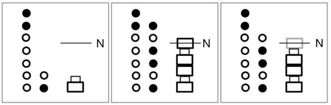
Figure 1: Example of how generation 1 is created in the Wright-Fisher model with efficiency with $s=0$. Black (resp. white) dots correspond to inefficient (resp. efficient) individuals. Generation 0 is represented by the leftmost column: $\lfloor xN_{x}\rfloor=5$ and $\lfloor N_{x}\rfloor=7$. The small (resp. large) rectangles represent the amount of resource consumed to produce an efficient (resp. inefficient) individual and have height 1 (resp. $1-\kappa$). The horizontal line represents the total amount of resource, $N$. The second panel corresponds to (M1) and $M_{1}=6$. The third panel, corresponds to (M2) and $M_{1}=5$ (the last individual is discarded).

Figure 1 shows how generation 1 is created in the Wright-Fisher model with efficiency (M1) or (M2) and Figure 2 shows a simulation of the model. There is a strong coupling between the population size and the frequency of efficient individuals: when $X_{n}=1$, $M_{n}=\lfloor N/(1-\kappa)\rfloor+1$ under (M1) ( $M_{n}=\lfloor N/(1-\kappa)\rfloor$ under (M2)) and when $X_{n}=0$, $M_{n}=N$.

The main difference between the two stopping rules lays in the fact that, under (M1), we can always create efficient or inefficient individuals. But, under (M2), if the amount of consumed resource is in $(N-1,N]$ we can only produce efficient individuals. Therefore, under the stopping rule (M2), being efficient could be advantageous (see Section 1.5).

Figure 2: Simulations of the model ((M1): left side panels and (M2): right side panels), for $N=5$, $\kappa=0.3$ and $s=0.1$. In the upper panels, the large (resp. small) rectangles represent the amount of resource consumed to produce an inefficient (resp. efficient) individual and the horizontal line has height $N$. The bottom panels represent $(M_{n},n\geq 0)$ and $(X^{(5)}_{n},n\geq 0)$ respectively. The dashed lines correspond to the bounds between which the population size can fluctuate.

1.3 A diffusion-approximation under assumption (M1)

Our first result (which will be proven is Section 2) provides a scaling-limit for the Wright-Fisher model, when the population size is large and time is measured in the evolutionary scale (i.e. time is re-scaled by $N$).

Theorem 1.

Fix $\kappa\in[0,1]$ and $\alpha\geq 0$. Let us consider a sequence of processes $\{(X^{(N)}_{\lfloor Nt\rfloor},t\geq 0),N\geq 1\}$, as in Definition 1 under (M1) and with neutral (if $s_{N}=\alpha/N=0$), or selective parental rule with selection coefficient $s_{N}=\alpha/N>0$, and such that $X^{(N)}_{0}$ converges towards $x\in(0,1)$ in distribution. Then the sequence $\{(X^{(N)}_{\lfloor Nt\rfloor},t\geq 0),N\geq 1\}$ converges weakly in the Skorokhod sense to the unique strong solution of the following stochastic differential equation (SDE)

$$\mathrm{d}X_{t}=-\alpha X_{t}(1-X_{t})\mathrm{d}t+\sqrt{X_{t}(1-X_{t})(1-\kappa X_{t})}\mathrm{d}B_{t},$$ (1.2)

where $B$ denotes a standard Brownian motion and with initial condition $X_{0}=x$.

The SDE (1.2) already appeared in [González Casanova et al.(2017)]. Such unique strong solution, we call it the Wright-Fisher diffusion with efficiency (M1) and from now on, it is denoted by $(X_{t},t\geq 0)$. Figure 3 shows some simulated trajectories of $(X_{t},t\geq 0)$ and $(X^{(N)}_{\lfloor Nt\rfloor},t\geq 0)$.

To obtain the diffusion approximation, time was re-scaled by $N$ and we assumed that the selection coefficient $s_{N}$ is of order $1/N$ (as in the classical Wright-Fisher model with selection). However, no re-scaling of the efficiency parameter $\kappa$ is needed.

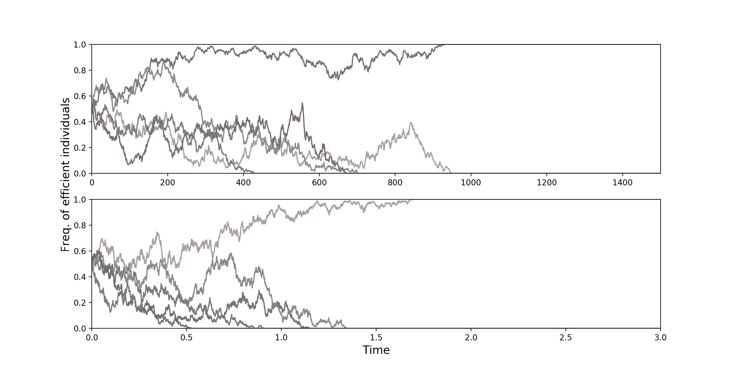
Figure 3: The upper panel shows some simulations of Wright-Fisher model with efficiency and the bottom panel some trajectories of the Wright-Fisher diffusion with efficiency (M1). The parameters are $N=500$, $x=0.5$, $\kappa=0.3$ and $\alpha=0.1$. In the upper panel, time is expressed in generations. In the bottom panel, 1 time-unit corresponds to $N$ generations.

The extra factor $(1-\kappa X_{t})$ in the infinitesimal variance is the main contribution of efficiency. Roughly speaking this term appears since, when the frequency of efficient individuals is $x$, the population size remains close to $N_{x}=N(1-\kappa x)^{-1}$ (Proposition 4 in Section 2)).

The diffusion $(X_{t},t\geq 0)$ has two boundaries, $0$ and $1$. We will show in Section 2 that when $\kappa\in[0,1)$ these boundaries are accessible (i.e. that they can be reached in finite time). We will also prove the following result.

Proposition 1.

Let $X=(X_{t},t\geq 0)$ be the unique strong solution of (1.2) and define the time to fixation as

$$T_{0,1}=\inf\{t\geq 0:X_{t}=0\textrm{ or }1\}.$$

Then,

• if $\kappa<1$ and $\alpha=0$, the expected time to fixation is given by

  $$\mathbb{E}[T_{0,1}|X_{0}=x]=2x\log\left(\frac{1-\kappa x}{x(1-\kappa)}\right)-\frac{2(1-x)}{1-\kappa}\log\left(\frac{1-x}{1-\kappa x}\right),$$ (1.3)

• if $\alpha>0$ and $\kappa<1$, then $\mathbb{E}[T_{0,1}|X_{0}=x]<\infty,$

• if $\kappa=1$ then $\mathbb{E}[T_{0,1}|X_{0}=x]=\infty$.

When $\kappa\in[0,1)$ absorption occurs in finite time. If $\alpha=0$, $(X_{t},t\geq 0)$ is a martingale, so the probability of fixation of the efficient individuals is equal to their initial frequency (as in the classical Wright-Fisher model). In other words, there is no advantage or disadvantage at the population level in being efficient. But the time to absorption increases with $\kappa$. This is not surprising, since the presence of inefficient individuals reduces the population size.

Let us denote by $(Y_{t},t\geq 0)$ the process $Y=1-X$, which corresponds to the (limiting) frequency of inefficient individuals. Define $\mathbb{P}_{y}\big{(}\{{\rm Fix.}\}\big{)}=\mathbb{P}(Y_{T_{0,1}}=1|Y_{0}=y)$, the probability of fixation of the inefficient individuals starting from $y\in(0,1)$. When $\alpha>0$ and $\kappa=0$, it is well known (see for instance Lemma 5.7 in [Etheridge (2011)]) that the probability of fixation of type 1 individuals is given by

$$\mathbb{P}_{y}\big{(}\{{\rm Fix.}\}\big{)}=\frac{1-\exp\{-2\alpha y\}}{1-\exp\{-2\alpha\}}.$$

Proposition 2.

The probability of fixation of the inefficient individuals in the Wright-Fisher diffusion with efficiency (M1), parametrised by $\kappa\in(0,1)$ and $\alpha\geq 0$ is given by

$$\mathbb{P}_{y}(\{{\rm Fix.}\}) = \left\{\begin{array}[]{ll}1-C_{\kappa,\alpha}(1-(1-\kappa(1-y))^{1-\frac{2\alpha}{\kappa}})&\textrm{if}\quad 2\alpha\neq\kappa,\\ 1-C_{\kappa,\alpha}\ln\left(\frac{1}{1-\kappa(1-y)}\right)&\textrm{if}\quad 2\alpha=\kappa,\\ \end{array}\right.$$

where $C_{\kappa,\alpha}$ is such that

$$C_{\kappa,\alpha}^{-1}=\left\{\begin{array}[]{ll}1-(1-\kappa)^{1-\frac{2\alpha}{\kappa}}&\textrm{if}\quad 2\alpha\neq\kappa,\\ \ln\left(\frac{1}{1-\kappa}\right)&\textrm{if}\quad 2\alpha=\kappa.\end{array}\right.$$

The proof of this Proposition can be found in Section 2.

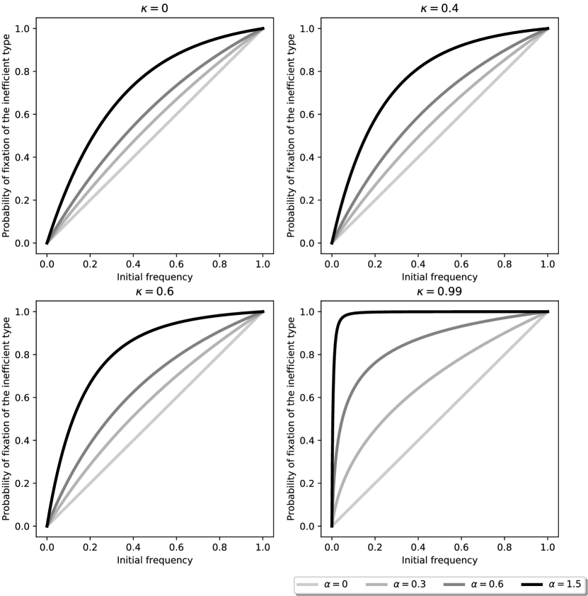
Figure 4: Probability of fixation of inefficient individuals for the Wright-Fisher diffusion with efficiency (stopping rule (M1)), for several combinations of $\kappa$ and $\alpha$.

As one can see in Figure 4, for a fixed value of $\alpha$, the probability of fixation of inefficient individuals increases when $\kappa$ increases. In other words, at the population level, being inefficient provides an advantage, since it increases the probability of fixation (compared to the classical Wright-Fisher model with the same selection coefficient).

Finally, we consider the case $\kappa=1$, which exhibits some interesting mathematical properties. It corresponds to the case where the cost of inefficient individuals is orders of magnitude larger than the cost of efficient individuals, in such a way that the efficiency parameter $\kappa_{N}$ tends to 1 as $N$ goes to infinity. In that case, $0$ is accessible but $1$ is not. However, it is still possible that $X$ takes the value 1 in the limit. In other words, the efficient individuals might still “go to fixation” after an infinite time. The first term of the right hand side of (1.3), which is related to absorption at $1$, goes to infinity when $\kappa$ goes to 1. But the second term, which is related to absorption in 0, converges to a finite value. The path behaviour is not easy to study using the classical theory of diffusions. Instead, we can use moment duality.

1.4 A genealogical process associated to the Wright-Fisher diffusion with efficiency (M1)

The Ancestral Selection/Efficiency Graph, that we introduce below, describes the genealogical structure associated to the Wright-Fisher model with efficiency (M1). It can be seen as an extension of the Ancestral Selection Graph (ASG) defined in [Krone and Neuhauser (1997a), Krone and Neuhauser (1997b)].

Definition 2.

Fix $n\in\mathbb{N},\kappa\in[0,1]$, $\alpha\geq 0$. The random marked directed graph $\mathcal{G}^{x}_{T}$, with parameters $T>0$ and $x\in[0,1]$, that we call the Ancestral Selection/Efficiency Graph (ASEG for short), is a continuous-time Markov process that can be constructed as follows. Let $Z_{t}$ denote the number of active vertices at time $t$ and assume that $Z_{0}=n$. If $Z_{t}=j$, then

1. (Coalescence event) at rate $j(j-1)/2$ two uniformly chosen active vertices become inactive and produce a new active vertex which is connected to both of them,

2. (Branching event) at rate $\alpha j$ an uniformly chosen active vertex becomes inactive and produces two new active vertices which are connected to it,

3. (Pairwise branching event) at rate $\kappa j(j-1)/2$ an uniformly chosen active vertex becomes inactive and produces two new active vertices which are connected to it,

4. (Coloring the tips) at time $T>0$, this procedure is stopped and each active vertex gets a type which is $0$ (efficient) with probability $x$ and $1$ (inefficient) otherwise,

5. (Coloring the inner vertices) each inactive vertex is of type $0$ if and only if there is no directed path from it to any vertex of type $1$.

Figures 5 and 6 represent the different types of events $(i)-(iii)$ and a realization of the ASEG respectively.

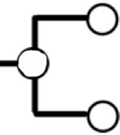
(a) coalescence

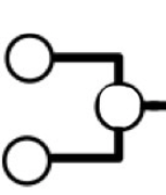
(b) branching

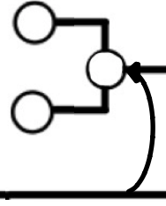
(c) pairwise branching

Figure 5: Events of the ASEG. Pairwise branching events occur at rate proportional to $j(j-1)/2$, which corresponds to choosing a pair of vertices (connected by an arrow in this representation), but only one of them becomes inactive and produces two new vertices.

The vertex counting process of the ASEG $Z=(Z_{t},t\geq 0)$ is a branching process with interactions, with parameters $(\alpha,1,\kappa)$, in the sense of [González Casanova et al.(2017)]. It is a birth-death process which goes from

$$j\text{ to}\left\{\begin{array}[]{ll}j+1&\textrm{ at rate }\alpha j+\kappa\frac{j(j-1)}{2},\\ j-1,&\textrm{ at rate }\frac{j(j-1)}{2}.\end{array}\right.$$

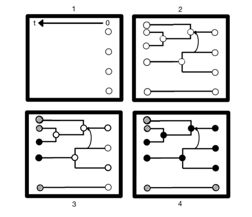
Figure 6: Realization of the ASEG. Panel 1 shows four active vertices at time 0. In panel 2, new vertices are produced according to rules $(i),(ii)$ and $(iii)$ of Definition 2. In panel 3, external vertices are colored according to rule $(iv)$ (type 1 is represented in black and type 0 in grey). In panel 4, individuals copy the type of their parents (the vertex to the left) following rule $(v)$.

Lemma 1.

The Wright-Fisher diffusion with efficiency $X$ defined as the unique strong solution of (1.2), with parameters $\alpha\geq 0$ and $\kappa\in[0,1]$ and the vertex counting process of the ASEG $Z$ defined above (with the same parameters), are moment duals, i.e. for all $x\in[0,1]$, $n\in\mathbb{N}$ and $t>0$,

$$\mathbb{E}_{x}[X_{t}^{n}]=\mathbf{E}_{n}[x^{Z_{t}}],$$

where $\mathbb{E}_{x}$ and $\mathbf{E}_{n}$ denote the expectations associated to the laws of $X$ and $Z$ starting from $x$ and $n$, respectively.

This result is a particular case of Theorem 2 in [González Casanova et al.(2017)]. For the sake of completeness, in Section 3 we provide its proof. Intuitively, the left-hand side corresponds to the probability that $n$ independent Bernoulli random variables with parameter $X_{T}$ are equal to 1. The right-hand side is the probability generating function of $Z_{t}$ evaluated at the initial frequency $x$ and is therefore related to the probability that the vertices in $\mathcal{G}^{x}_{T}$ are of type 1. Lemma 1 is surprising, since we can prove analytically that the ASEG is the moment dual of the Wright-Fisher diffusion with efficiency, but there does not seem to be a transparent mapping between the events of the two processes. We refer the reader to Section 3 for a more detailed study of the ASEG, which allows us to understand the path behaviour of the Wright-Fisher diffusion with efficiency (M1), when $\kappa=1$.

1.5 A diffusion-approximation under assumption (M2)

Finally, we study the scaling limit of the frequency process of efficient individuals under (M2), when $\kappa$ is a rational number. This assumption is interesting since it has natural interpretation: $\kappa=a/b$ means that $a$ inefficient individuals can be created with the amount of resource needed to produce $b$ efficient individuals. The case when $\kappa$ is irrational seems to be more involved. Note that, when $\kappa=1$, both stopping rules (M1) and (M2) are exactly the same since, in generation $g$, we stop producing new individuals when we have produced exactly $N$ inefficient individuals (the efficient individuals do not contribute to the cost $C_{(g,i)}$)

Theorem 2.

Fix $\alpha\geq 0$ and let $\kappa$ be a rational number in $[0,1)$. Let us consider a sequence of processes $\{(X^{(N)}_{\lfloor Nt\rfloor},t\geq 0),N\geq 1\}$, as in Definition 1, under (M2) and with neutral ($s_{N}=\alpha/N=0$) or selective ($\alpha>0$) parental rule, with selection coefficient $s_{N}=\alpha/N$ and such that $X^{(N)}_{0}$ converges towards $x\in(0,1)$ in distribution. Then the sequence $\{(X^{(N)}_{\lfloor Nt\rfloor},t\geq 0),N\geq 1\}$ converges weakly in the Skorokhod sense to the unique strong solution of one of the following SDE’s:

• if $\kappa=a/b\in(0,1/2)$ for some relative primes $a,b\in\mathbb{N}$, then

  $$\mathrm{d}X_{t}=(-\alpha+\kappa(1-\kappa X_{t}))X_{t}(1-X_{t})\mathrm{d}t+\sqrt{X_{t}(1-X_{t})(1-\kappa X_{t})}\mathrm{d}B_{t},$$ (1.5)

• if $1-\kappa=1/b\in(0,1)$ for some $b\in\mathbb{N}$, then

  $$\mathrm{d}X_{t} = \left(-\alpha+(1-\kappa)(1-\kappa X_{t})\sum_{r=2}^{b-1}(1-X_{t}^{r})\right)X_{t}(1-X_{t})\mathrm{d}t$$ (1.6)

  $$+\sqrt{X_{t}(1-X_{t})(1-\kappa X_{t})}\mathrm{d}B_{t},$$

• if $1-\kappa=a/b\in(0,1/2)$ for some relative primes $a,b\in\mathbb{N}$, then

  $$\mathrm{d}X_{t} = \left(-\alpha+(1-\kappa X_{t})\sum_{i=1}^{m}c_{i}(1-X_{t}^{i})\right)X_{t}(1-X_{t})\mathrm{d}t$$ (1.7)

  $$+\sqrt{X_{t}(1-X_{t})(1-\kappa X_{t})}\mathrm{d}B_{t},$$

  where $m=\lfloor(1-\kappa)^{-1}\rfloor$, $c_{m}=1-ma/b$ and $c_{i}=a/b$ for all $i=1,2,...,m-1$.

In the three cases $B$ denotes a standard Brownian motion and the initial condition is $X_{0}=x$.

This result is proven in Section 4. The unique strong solution of each of the above SDEs is called the Wright-Fisher diffusion with efficiency (M2) and denoted by $(X_{t},t\geq 0)$. When $\alpha=0$, the first term in the right-hand side of the three SDEs (the “deterministic part”) is positive. As a consequence, the efficient individuals have some “advantage”, in the sense that their probability of fixation is higher than their initial frequency. This phenomenon can be explained by the fact that when the amount of consumed resource is in $(N-1,N]$, only efficient individuals can be produced. In the three cases, when $\alpha=0$, the diffusions obtained can be interpreted as random time-changes of some known diffusions. To be more precise, in all cases above we have

$$X_{t}=\tilde{X}_{\int_{0}^{t}(1-\kappa X_{s})\mathrm{d}s},\qquad 0\leq t\leq T_{0,1},$$

where the $\tilde{X}$ is the Wright-Fisher diffusion with selection (i.e $\kappa=0$) in the case $(i)$, or the Wright-Fisher diffusion with frequency dependent selection (see equation (1) of [González Casanova and Spano (2018)]) in the cases $(ii)$ and $(iii)$.

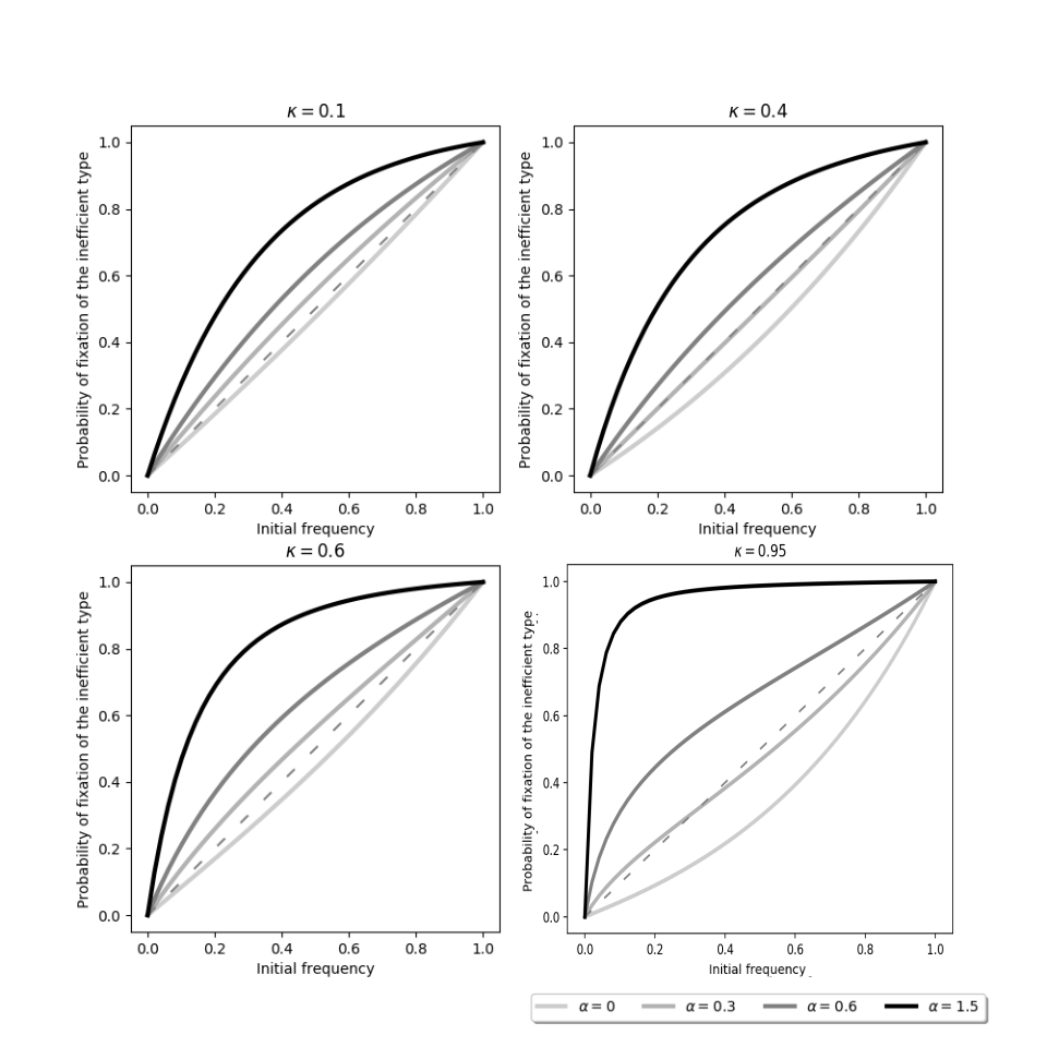
Figure 7: Probability of fixation of inefficient individuals for the Wright-Fisher diffusion with efficiency (M2), for several combinations of $\kappa$ and $\alpha$. The dashed line corresponds to $y=x$, which is the probability of fixation in the neutral Wright-Fisher model. To compute the probability of fixation, the scale function was integrated numerically, using Scipy library for Python.

When $s>0$, the sign of the first term in the three SDEs depends on the relative values of $\kappa,\alpha$ and $X_{t}$. For some values of $\alpha$ and $\kappa$, the drift term is negative when $X_{t}$ is close to 1 and positive when $X_{t}$ is close to 0. This phenomenon is called balancing selection (as selection “pushes” the frequency process towards intermediary values).

For the sake of brievity, we now focus on the case $(i)$. We prove in Section 4 that both boundaries $0$ and $1$ are accessible, that the expected time to fixation is finite and that we have the following result.

Proposition 3.

The probability of fixation of the inefficient individuals in the Wright-Fisher diffusion with efficiency (M2) parametrised by $\kappa=a/b\in(0,1/2)$ for some relative primes $a,b\in\mathbb{N}$ and $\alpha\geq 0$ is given by

$$\mathbb{P}_{y}(\{{\rm Fix.}\})=\frac{\int_{1-y}^{1}\exp(-2\kappa u)(1-\kappa u)^{-2\alpha/\kappa}\mathrm{d}u}{\int_{0}^{1}\exp(-2\kappa u)(1-\kappa u)^{-2\alpha/\kappa}\mathrm{d}u}.$$

As we can observe in Figure 7, for a fixed $\kappa$, if $\alpha$ is small, $\mathbb{P}_{y}(\{{\rm Fix.}\})<y$. The latter means that, at the population level, efficient individuals have some advantage (as in the case (M2), with $\alpha=0$). However, when $\alpha$ is large enough (for example when $\kappa=0.4$ and $\alpha=1.5$), $\mathbb{P}_{y}(\{{\rm Fix.}\})>y$, meaning that the inefficient individuals have some advantage at the population level, as in the case (M1). Finally, in some cases (for example $\kappa=0.95$ and $\alpha=0.3$ in Figure 7), we can see the effect of the balancing selection. Indeed, when we compare the fixation probabilities to the ones of the Wright-Fisher model with selection, if the initial frequency of inefficient individuals is low, they have some advantage. On the contrary, if their initial frequency is high, they have some disadvantage. Recall that, to observe this effect in a finite population of size $N$, we need a small selection coefficient ($s_{N}=\alpha/N$) compared to the efficiency parameter $\kappa$.

1.6 Discussion and open problems

To summarize, we discuss the evolutionary consequences of efficiency by using an extension of the Wright-Fisher model in which different types of individuals need different amounts of resource to reproduce. We consider two variations of the model, depending on the rule that is used to complete each generation. Under assumption (M2), efficiency provides some advantage at the population level (see Theorem 2). However, the main contribution of this work is that inefficiency can be part of the advantage of an emerging trait. Imagine a situation in which two types of individuals with different strategies co-exist. A beneficial mutation is more likely to be fixed in the population if it arises in an inefficient individual. In other words, inefficiency acts as a promoter of selective advantage. This is always the case for rule (M1) and it is also true for rule (M2) if the selection parameter is large enough (see Figures 4 and 7). This positive correlation between inefficiency and fixation probability occurs whether the beneficial mutation carried by the inefficient individuals is due to a physiological trade-off or is an independent mutation (maybe on a different gene).

The Wright-Fisher diffusion with efficiency (M1) has a moment dual, which is a branching-coalescing process, the ASEG. This result, which generalises the ASG, comes from analytic manipulations, but still requires a transparent interpretation in terms of discrete models. It is possible to construct a Moran model with selection where individuals choose a certain number of potential parents and such that, if time is reverted, it contains the ASG (see [Mano (2009), Lenz et al. (2015), Kluth and Baake (2013)]). However, it is not clear how we can extend this construction to the ASEG and how to interprete the pairwise branching events. This is an interesting open question. In the case of assumption (M2), we were not able to find an associated genealogical process. It is also an open question, possibly related to the first one.

Finally, efficiency can act as a mechanism of balancing selection, which is considered to be one of the most powerful evolutionary forces maintaining polymorphism (see for example [Turelli and Barton (2004), Fitzpatrick et al. (2007)] or [Brisson (2018)] for a more recent review). Many different mechanisms of balancing selection have been suggested in the literature, such as within niche competition, heterozygote advantage, self-incompatibility between mating types and host-parasite or prey-predator interactions (see [Brisson (2018)] and the references therein), but to our knowledge this is the first work in which it arises from within-species differences in resource consumption strategies. The consequences of these effects still have to be studied especially by means of experiments.

2 Scaling limit of model (M1)

In order to prove Theorem 1, we first deduce the following proposition which is crucial for determining the scaling limits of the Wright-Fisher model with efficiency. In particular, it says that the total number of individuals in a generation $n+1$ is close to its expectation given the frequency of efficient individuals in generation $n$.

Proposition 4.

In the Wright-Fisher model with efficiency, with neutral parental rule ($s=0$), and with stopping rule (M1) or (M2), parametrised by $\kappa\in[0,1]$, given $X^{(N)}_{n}=x\in[0,1]$, for every $a\in(-1/2,0)$, we have

$$\lim_{N\rightarrow\infty}\inf_{x\in(0,1)}\mathbb{P}\left(\frac{M_{n+1}}{N_{x}}\in[1-N^{a},1+N^{a}]\right)=1.$$

Proof.

Let $\{B_{i};i\geq 1\}$ be a sequence of i.i.d. Bernoulli random variables with parameter $x$. For every $a\in(-1/2,0)$, using the definition of $N_{x}$ (1.1), we get

$$\begin{split}\mathbb{P}\Bigg{(}\frac{M_{n+1}}{N_{x}}\leq 1-N^{a}\Bigg{)}&=\mathbb{P}\Big{(}C_{(n+1,\lfloor N_{x}(1-N^{a})\rfloor)}\ {\geq}\ N\Big{)}\\ &=\mathbb{P}\left(\lfloor N_{x}(1-N^{a})\rfloor-\kappa\sum_{i=1}^{\lfloor N_{x}(1-N^{a})\rfloor}B_{i}\ {\geq}\ N\right)\\ &\leq\mathbb{P}\left(N_{x}\Big{(}\kappa x-N^{a}\Big{)}\ {\geq}\ \kappa\sum_{i=1}^{\lfloor N_{x}(1-N^{a})\rfloor}B_{i}\right).\end{split}$$

Adding and subtracting $\kappa xN_{x}N^{a}$, using (1.1) and then adding and subtracting $\kappa x\lfloor N_{x}(1-N^{a})\rfloor$ yields

$$\begin{split}&\mathbb{P}\Bigg{(}\frac{M_{n+1}}{N_{x}}\leq 1-N^{a}\Bigg{)}\leq\mathbb{P}\left(\kappa xN_{x}(1-N^{a})-N^{1+a}\ {\geq}\ \kappa\sum_{i=1}^{\lfloor N_{x}(1-N^{a})\rfloor}B_{i}\right)\\ &=\mathbb{P}\left(-N^{1+a}+\kappa x\Big{(}N_{x}(1-N^{a})-\lfloor N_{x}(1-N^{a})\rfloor\Big{)}\ {\geq}\ \kappa\sum_{i=1}^{\lfloor N_{x}(1-N^{a})\rfloor}B_{i}-\kappa x\lfloor N_{x}(1-N^{a})\rfloor\right)\\ &\leq\mathbb{P}\left(-N^{1+a}+1\ {\geq}\ \kappa\sum_{i=1}^{\lfloor N_{x}(1-N^{a})\rfloor}(B_{i}-x)\right)\\ &\leq\mathbb{P}\left(\kappa\left|\sum_{i=1}^{\lfloor N_{x}(1-N^{a})\rfloor}(B_{i}-x)\right|\ {\geq}\ N^{1+a}+1\right).\end{split}$$

For the upper bound, a similar strategy can be used to get

$$\begin{split}\mathbb{P}\left(\frac{M_{n+1}}{N_{x}}\geq 1+N^{a}\right)&=\mathbb{P}\Big{(}C_{(n+1,\lfloor N_{x}(1+N^{a})\rfloor)}<N\Big{)}\\ &\leq\mathbb{P}\left(N_{x}\Big{(}\kappa x+N^{a}\Big{)}>-1+\kappa\sum_{i=1}^{\lfloor N_{x}(1+N^{a})\rfloor}B_{i}\right)\\ &\leq\mathbb{P}\left(\kappa\left|\sum_{i=1}^{\lfloor N_{x}(1+N^{a})\rfloor}(B_{i}-x)\right|>N^{1+a}+2\right).\end{split}$$

Next, since $B_{i}-x$ is a centered random variable with $\mathbb{V}ar[B_{i}]=x(1-x)$, we have

$$\begin{split}\mathbb{V}ar\left[\sum_{i=1}^{\lfloor N_{x}(1-N^{a})\rfloor}(B_{i}-x)\right]&\leq\sum_{i=1}^{\lfloor N_{x}(1+N^{a})\rfloor}\mathbb{V}ar[B_{i}-x]\\ &=\frac{N}{1-\kappa x}(1+N^{a})x(1-x)\\ &\leq N(1+N^{a}).\end{split}$$

In both cases, from Tchebycheff’s inequality we obtain

$$\begin{split}\lim_{N\rightarrow\infty}\sup_{x\in(0,1)}&\mathbb{P}\left(\frac{M_{n+1}}{N_{x}}\notin[1-N^{a},1+N^{a}]\right)\\ &\leq\lim_{N\rightarrow\infty}\sup_{x\in(0,1)}\mathbb{P}\left(\kappa\left|\sum_{i=1}^{\lfloor N_{x}(1-N^{a})\rfloor}(B_{i}-x)\right|>N^{1+a}+1\right)\\ &\leq\lim_{N\rightarrow\infty}\frac{N(1+N^{a})}{(N^{(1+a)}+1)^{2}}=\lim_{N\rightarrow\infty}N^{1-2(1+a)}=0,\end{split}$$

where we have used that $1-2(1+a)<0$ since $a\in(-1/2,0)$. The proof of this proposition now follows. ∎

Proof of Theorem 1.

Classical results for SDEs with Hölder continuous coefficients provide that (1.2) has a unique strong solution (see for instance Theorem 2 in [González Casanova et al.(2017)]). We denote by $\mathcal{A}$ the infinitesimal generator of the Wright-FIsher diffusion with efficiency. Its domain contains the set of continuously twice differentiable functions on $[0,1]$, here denoted by $C^{2}([0,1])$, and for every $f$ in $C^{2}([0,1])$, and for every $x\in[0,1]$, we have

$$\mathcal{A}f(x)=-\alpha x(1-x)f^{\prime}(x)+x(1-x)(1-\kappa x)f^{\prime\prime}(x).$$ (2.8)

Recall that, given $X^{(N)}_{0}=x$ and $M_{1}=m$, $mX_{1}^{(N)}$ follows a binomial distribution with parameters $m$ and $(1-s_{N})x/(1-s_{N}x)$, using Taylor’s expansions, as in the classical Wright-Fisher model with selection, we have

$$N\mathbb{E}\Big{[}X_{1}^{(N)}-x|X_{0}^{(N)}=x,M_{1}=m\Big{]} = -\alpha x(1-x)+o(1)$$

$$N\mathbb{E}\Big{[}(X_{1}^{(N)}-x)^{2}|X_{0}^{(N)}=x,M_{1}=m\Big{]} = \frac{N}{m}x(1-x)+o(1),$$

where $N/m\leq 1$. If we take $f\in C^{2}([0,1])$, $x\in[0,1]$, $a\in(-1/2,0)$ and using Proposition 4, the discrete generator of $X^{(N)}_{\lfloor Nt\rfloor}$ satisfies

$$\begin{split}A^{N}f(x):=&N\mathbb{E}\Big{[}f(X_{1}^{(N)})-f(x)|X_{0}^{(N)}=x\Big{]}\\ =&N\mathbb{E}\Big{[}X_{1}^{(N)}-x|X_{n}^{(N)}=x\Big{]}f^{\prime}(x)+N\mathbb{E}\Big{[}(X_{1}^{(N)}-x)^{2}|X_{0}^{(N)}=x\Big{]}f^{\prime\prime}(x)+o(1)\\ =&-\alpha x(1-x)f^{\prime}(x)\\ &+N\mathbb{E}\Big{[}(X_{1}^{(N)}-x)^{2}\Big{|}X_{0}^{(N)}=x,M_{1}\in[N_{x}(1-N^{a}),N_{x}(1+N^{a})]\Big{]}f^{\prime\prime}(x)+o(1)\\ =&-\alpha x(1-x)f^{\prime}(x)+\frac{N}{\lfloor N_{x}\rfloor}x(1-x)f^{\prime\prime}(x)+o(1)\\ =&-\alpha x(1-x)f^{\prime}(x)+x(1-x)(1-\kappa x)f^{\prime\prime}(x)+o(1)\underset{N\to\infty}{\longrightarrow}\mathcal{A}f(x),\end{split}$$

where the term $o(1)$ depends on $x$ but converges to 0 uniformly in $x$. Since all the processes involved are Feller taking values on $[0,1]$ and the convergence of the generators is uniform by Proposition 4, then the result follows from Lemma 17.25 of [Kallemberg (1997)]. ∎

The rest of this section is dedicated to the study of the Wright-Fisher diffusion with efficiency. We start by proving the following proposition.

Lemma 2.

Let $X=(X_{t},t\geq 0)$ be the unique strong solution of (1.2), the following statements holds.

• For $\alpha\geq 0$ and $\kappa<1$, the boundary points $0$ and $1$ are accesible.

• For $\kappa=1$ and $\alpha\geq 0$, the boundary $1$ is not accesible and the boundary $0$ is accesible.

Proof.

We start by introducing the Wright-Fisher diffusion with selection parameter $c\in\mathbb{R}$ as the unique strong solution of

$$\mathrm{d}\hat{Y}^{(c)}_{t}=c\hat{Y}^{(c)}_{t}\Big{(}1-\hat{Y}^{(c)}_{t}\Big{)}\mathrm{d}t+\sqrt{\hat{Y}^{(c)}_{t}\Big{(}1-\hat{Y}^{(c)}_{t}\Big{)}}\mathrm{d}B_{t},$$ (2.9)

where $B$ denotes a standard Brownian motion.

We first deal with the case $\alpha\geq 0$ and $\kappa\in(0,1)$. To do so, we use a stochastic domination argument. Let us introduce the following diffusion $\overline{Y}^{(c)}=(\overline{Y}^{(c)}_{t},t\geq 0)$ which is obtained as a random time change of $\hat{Y}^{(c)}$, that is to say, for the clock

$$A_{t}=\int_{0}^{t}\frac{\mathrm{d}s}{1-\kappa\hat{Y}^{(c)}_{s}},\qquad\textrm{for}\quad t\geq 0,$$

we introduce $\overline{Y}^{(c)}_{t}=\hat{Y}^{(c)}_{\theta_{t}},$ for $t\geq 0$ where $\theta_{t}=\inf\{u:A_{u}>t\}$ is the right-continuous inverse of the clock $A$. Using (2.9), we observe that $\overline{Y}^{(c)}$ satisfies the following SDE

$$\mathrm{d}\overline{Y}^{(c)}_{t}=c\overline{Y}^{(c)}_{t}\Big{(}1-\overline{Y}^{(c)}_{t}\Big{)}\Big{(}1-\kappa\overline{Y}^{(c)}_{t}\Big{)}\mathrm{d}t+\sqrt{\overline{Y}^{(c)}_{t}\Big{(}1-\overline{Y}^{(c)}_{t}\Big{)}\Big{(}1-\kappa\overline{Y}^{(c)}_{t}\Big{)}}\mathrm{d}\beta_{t},$$

where $\beta=(\beta_{t},t\geq 0)$ is a standard Brownian motion. Since, for every $t\geq 0$, we have

$$\theta_{t}=\int_{0}^{t}\Big{(}1-\kappa\overline{Y}^{(c)}_{s}\Big{)}\mathrm{d}s\in[(1-\kappa)t,t],$$

and $Y^{(c)}$ goes to fixation in finite time a.s. (see for instance equation (3.6) in [Ewens (1963)]), we deduce that this is also the case for $\overline{Y}^{(c)}$. In other words, both boundaries are accessible for $\overline{Y}^{(c)}$ for every $c\in\mathbb{R}$.

Finally, since for any fixed $\alpha>0$, we have that a.s.

$$\overline{Y}^{(-\alpha)}_{t}\geq X_{t}\geq\overline{Y}^{(\alpha/(\kappa-1))}_{t},\qquad t\geq 0,$$

and for $\alpha=0$, $X\equiv\overline{Y}^{(0)}$, we conclude that the boundaries $\{0,1\}$ are also accessible for $X$.

For the case $\alpha=0$ and $\kappa=1$, we use the following integral test which says that the boundary $a$ is accessible if and only if

$$\int_{x_{0}}^{a}M(u)\mathrm{d}S(u)<\infty$$

where $M$ and $S$ denote the speed measure and the scale function associated to $X$ (see for instance Chap. 8 in [Ethier and Kurtz (1986)]). In our case both functions can be computed explicitly. Indeed, the scale function is proportional to the identity and the speed measure satisfies

$$M(x)=\int_{x_{0}}^{x}\frac{1}{u(1-u)^{2}}\mathrm{d}u=\frac{1}{1-x}-\log(1-x)+\log(x)+c(x_{0}),$$ (2.10)

where $c(x_{0})$ is a constant that only depends on $x_{0}$. We have

$$\int_{x_{0}}^{1}\left(\frac{1}{1-u}-\log(1-u)+\log(u)\right)\mathrm{d}u=\infty$$

while

$$\int_{0}^{x_{0}}\left(\frac{1}{1-u}-\log(1-u)+\log(u)\right)\mathrm{d}u<\infty,$$

so 1 is not accessible and 0 is accessible. The case $\alpha>0$ and $\kappa=1$, follows directly from a stochastic domination argument by the neutral Wright-Fisher diffusion with efficiency $\kappa=1$ (and $\alpha=0$) studied above. ∎

Proof of Proposition 1.

We first deduce part $(i)$, i.e. we compute the expected time to fixation for the case $\alpha=0$ and $\kappa\in(0,1)$. To do so, we use Green’s function (see for instance Theorem 3.19 in [Etheridge (2011)]) i.e.

$$\mathbb{E}\Big{[}T_{0,1}|X_{0}=x\Big{]}=\int_{0}^{1}G(x,u)\mathrm{d}u,$$

where the Green’s function $G$ is such that

$$G(x,u)=\left\{\begin{array}[]{ll}\frac{2x}{u(1-\kappa u)}&\textrm{ for }x<u<1,\\ \textrm{ }\\ \frac{2(1-x)}{(1-u)(1-\kappa u)}&\textrm{ for }0<u<x,\end{array}\right.$$ (2.11)

implying that the expected time to fixation satisfies

$$\begin{split}\mathbb{E}\Big{[}T_{0,1}|X_{0}=x\Big{]}&=-2x\Big{(}\log(x)+\log(1-\kappa)-\log(1-\kappa x)\Big{)}\\ &\hskip 56.9055pt-2(1-x)\left(\frac{\log(1-x)}{1-\kappa}-\frac{\log(1-\kappa x)}{1-\kappa}\right).\end{split}$$

For part $(ii)$, i.e. when $\alpha>0$ and $\kappa\in(0,1]$, the Green’s function is such that for

$$G(x,u)=\left\{\begin{array}[]{ll}\frac{2(S(x)-S(0))}{(S(1)-S(0))S^{\prime}(u)}\frac{S(1)-S(u)}{u(1-u)(1-\kappa u)}&\textrm{ for }x<u<1,\\ \textrm{ }\\ \frac{2(S(1)-S(x))}{(S(1)-S(0))S^{\prime}(u)}\frac{S(u)-S(0)}{u(1-u)(1-\kappa u)}&\textrm{ for }0<u<x,\end{array}\right.$$

where $S$ is the scale function and satisfies for $x\in[0,1]$

$$S(x)=\int_{0}^{x}\exp\left\{\frac{2\alpha}{\kappa}\int_{\theta}^{u}\frac{\mathrm{d}v}{\frac{1}{\kappa}-v}\right\}\mathrm{d}u\ =\left\{\begin{array}[]{ll}K\left(1-\left(1-\kappa x\right)^{1-\frac{2\alpha}{\kappa}}\right)&\textrm{for }\kappa\neq 2\alpha\\ K\ln\left(\frac{1}{1-\kappa x}\right)&\textrm{for }\kappa=2\alpha,\end{array}\right.$$

where $\theta$ is an arbitrary positive number and $K$ is a constant that depends on $(\kappa,\alpha,\theta)$. To determine whether the Green’s function is integrable on $[0,1]$, it is enough to study its behavior near the boundaries 0 and 1. Indeed, for $u$ close to 0, we have

$$G(x,u)\sim\frac{2(S(1)-S(x))}{(S(1)-S(0))}\frac{1}{(1-u)(1-\kappa u)},$$

so the function $u\mapsto G(x,u)$ is always integrable in a neighborhood of 0. Moreover, when $u$ is close to 1, we get

$$G(x,u)\sim\frac{2(S(x)-S(0))}{(S(1)-S(0))}\frac{1}{u(1-\kappa u)},$$

so the function $u\mapsto G(x,u)$ is integrable in a neighborhood of 1 if $\kappa<1$ and is not integrable if $\kappa=1$, which completes the proof. ∎

Proof of Proposition 2.

We use Lemma 2. In fact, as both boundaries are accessible, the probability of fixation of the efficient individuals with selective disadvantage is given by

$$\mathbb{P}_{y}(\{{\rm Fix.}\}) = \mathbb{P}(Y_{T_{0,1}}=1|Y_{0}=y)$$

$$= \mathbb{P}(X_{T_{0,1}}=0|X_{0}=1-y)=\frac{S(1)-S(1-y)}{S(1)-S(0)}$$

$$= \left\{\begin{array}[]{ll}C_{\kappa,\alpha}(1-(1-\kappa x)^{1-\frac{2\alpha}{\kappa}})&\textrm{if}\quad 2\alpha\neq\kappa,\\ C_{\kappa,\alpha}\ln\left(\frac{1}{1-\kappa x}\right)&\textrm{if}\quad 2\alpha=\kappa,\\ \end{array}\right.$$

where $C_{\kappa,\alpha}=S(1)^{-1}$ (see for example Lemma 3.14 in [Etheridge (2011)]).

∎

3 The Ancestral Selection/Efficiency Graph

3.1 Properties of the ASEG

This section is devoted to a more detailed study of the vertex counting process of the ASEG, $Z$.

When $\kappa<1$, it can be shown using standard techniques for birth-death processes, that when $\alpha>0$, the states $\{1,2,3,\ldots\}$ are positive recurrent and the state $\{0\}$ is not accessible. When $\alpha=0$, the states $\{2,3,\ldots\}$ are positive recurrent, $\{0\}$ is not accessible and $\{1\}$ is absorbing (see Proposition 1 in [González Casanova et al.(2017)] for a detailed proof of the general case). In the ASEG, there are coalescence events, which correspond to negative jumps of size 1 of $Z$, and occur at the same rate as in the Kingman coalescent case. But there are also two types of events that create new vertices: branching events (which are related to selection, since their rate depends on $\alpha$) and pairwise branching events (which are related to efficiency, since their rate depends on $\kappa$). They correspond to positive jumps of size 1 of $Z$ and, therefore, $Z$ is not monotone as opposed to the block counting process of the Kingman coalescent which is monotone decreasing. Having these positive jumps of size one resembles the behavior of the vertex counting process of the ASG. When $\alpha=0$, by analogy with the ASG, the pairwise branching events, together with the coloring rule, seem to favor the creation of efficient individuals (as if there was some selection). However, the model is neutral and for every $t>0$, $\mathbb{E}_{x}[X_{t}]=x$. This apparent paradox has the following nice interpretation. If $X$ starts at $x\in(0,1)$, it will eventually get absorbed in $1$ (with probability $x$) or $0$ (with probability $1-x$). However, the process will go faster to 0 than to 1, since the term $(1-\kappa x)$ slows the process down much more when $x$ is close to 1 than when its closer to zero. This explains why, for small times, it is more likely to sample inefficient individuals but this apparent advantage vanishes for large times since $X$ will have enough time to reach one of the two absorbing states.

The study of the case $\kappa=1$ is particularly interesting, since it allows to understand the path behaviour of the Wright-Fisher model with efficiency under (M1) when $\kappa=1$, which was not possible to study using the classical theory of diffusions.

Theorem 3.

If $\kappa=1$, the block counting process of the ASEG $Z$ is transient if and only if $\alpha\in(1/2,\infty)$. If $\alpha\in[0,1/2)$ it is positive recurrent and has a unique stationary distribution $\mu$, which is a Sibuya distribution, i.e it is characterized as follows

$$\sum_{j\geq 1}x^{j}\mu(j)=1-(1-x)^{1-2\alpha}.$$

This theorem, together with the moment duality, allows us to describe the limiting behavior of $X$ and the distribution of the random variable $X_{\infty}:=\lim_{t\to\infty}X_{t}$ (in distribution), when $\kappa=1$ and $\alpha\in[0,1/2)$.

Corollary 1.

The Wright-Fisher diffusion with efficiency $X$ converges almost surely to zero if $\kappa=1$ and $\alpha>1/2$. Moreover if $\kappa=1$ and $\alpha\in[0,1/2)$, then $X_{\infty}$ follows a Binomial distribution with parameter $1-(1-x)^{1-2\alpha}$.

When $\kappa=1$ and $\alpha=1/2$, the path behavior of $X$ is not so easy to study. We conjecture that in this case the block counting process of the ASEG is null recurrent and $X$ goes to zero almost surely.

3.2 Proofs

This section is devoted to the proofs of the results presented in Sections 1.4 and 3.1.

Proof of Lemma 1.

Let us denote by $\mathcal{Q}$ the generator of $Z$ which satisfies, for any $f$ bounded function of IN, that

$$\mathcal{Q}f(n)=\left(\alpha n+\frac{n(n-1)}{2}\kappa\right)\Big{(}f(n+1)-f(n)\Big{)}+\frac{n(n-1)}{2}\Big{(}f(n-1)-f(n)\Big{)}.$$

Recall that $\mathcal{A}$ denotes the infinitesimal generator of the Wright-Fisher diffusion with efficiency which satisfies (2.8) for any function in $C^{2}([0,1])$. We consider a function $h$ which is defined on $[0,1]\times\mbox{\rm IN}$ and such that $h(x,n)=x^{n}$.

Since $h(x,n)$ and $\mathbb{E}[x^{Z_{t}}]$ are polynomials on $x$ and $h(x,n)$ and $\mathbb{E}[X_{t}^{n}]$ are bounded functions of $n$, we deduce from Proposition 1.2 of [Jensen and Kurt (2014)] that our claim follows if we show that for all $x\in[0,1]$ and $n\in\mbox{\rm IN}$, the following identity holds

$$\mathcal{A}h(x,n)=\mathcal{Q}h(x,n).$$

We observe that in the left-hand side of the above identity, $\mathcal{A}$ acts on $h$ (seen as a function of $x$) and in the right-hand side $\mathcal{Q}$ acts on $h$ (seen as a function of $n$).

Hence from the definitions of $\mathcal{A}$ and $\mathcal{Q}$, it is clear that for all $x\in[0,1]$ and $n\in\mbox{\rm IN}$, we have

$$\begin{split}\mathcal{A}h(x,n)&=-\alpha x(1-x)\frac{\partial h(x,n)}{\partial x}+x(1-x)(1-\kappa x)\frac{\partial^{2}h(x,n)}{\partial x^{2}}\\ &=-\alpha x(1-x)nx^{n-1}+x(1-x)(1-\kappa x)\frac{n(n-1)}{2}x^{n-2}\\ &=(\alpha n+\frac{n(n-1)}{2}\kappa)(x^{n+1}-x^{n})+\frac{n(n-1)}{2}(x^{n-1}-x^{n})\\ &=(\alpha n+\frac{n(n-1)}{2}\kappa)(h(x,n+1)-h(x,n))+\frac{n(n-1)}{2}(h(x,n-1)-h(x,n))\\ &=\mathcal{Q}h(x,n),\end{split}$$

which completes the proof. ∎

Proof of Theorem 3.

We start by proving that $Z$ is transient if and only if $\alpha>1/2$ and $Z$ positive recurrent if $\alpha\in[0,1/2)$. To do so, we study its jump chain denoted by $S=(S_{n},n\geq 0)$ (see for instance 3.4.1 in [Norris (1998)]). Observe that $S$ is a birth-death Markov chain with transition probabilities given by

$$\Pi_{k,j}=\mathbb{P}(S_{1}=j|S_{0}=k)=\left\{\begin{array}[]{ll}\frac{1}{2}+\frac{\alpha}{2k}+O(k^{-2})&\textrm{ for }j=k+1,\\ \textrm{ }\\ \frac{1}{2}-\frac{\alpha}{2k}+O(k^{-2})&\textrm{ for }j=k-1.\end{array}\right.$$

From Theorem 3 in [Harris (1952)] (see also [Lamperti (1960)]) we know that $S$ is transient if and only if $\alpha>1/2$ which implies the first part of our claim.

For the second part, we use the Foster-Lyapunov criteria (see for instance Proposition 1.3 in [Hairer (2016)]) with the Lyapunov function $f(n)=\ln(n)$. Recall that $\mathcal{Q}$ is the generator of $Z$. Using Taylor’s expansion

$$\begin{split}\mathcal{Q}\ln(n)&=\alpha n\ln\left(1+\frac{1}{n}\right)+\binom{n}{2}\left(\ln\left(1-\frac{1}{n}\right)+\ln\left(1+\frac{1}{n}\right)\right)\\ &=\alpha\left(1-\frac{1}{2n}\right)-1/2\left(1+\frac{1}{n}\right)+O(n^{-2}).\end{split}$$

That is to say

$$\mathcal{Q}\ln(n)\leq-\epsilon,$$

for all but finitely many values of $n$, and any $\epsilon\in(0,1/2-\alpha)$. According to Foster-Lyapunov criteria $Z$ is positive recurrent and there exists a unique invariant distribution here denoted by $\mu$. The moment duality property (Lemma 1) implies that

$$\mathbb{E}[X_{\infty}^{n}|X_{0}=x]=\sum_{j\geq 1}x^{j}\mu(j),\qquad\textrm{for all}\quad n\geq 0.$$

Therefore $X_{\infty}$ must be a Bernoulli distribution and we have

$$\sum_{j\geq 1}x^{j}\mu(j)=\mathbb{P}_{x}(X_{\infty}=1)=\mathbb{P}_{1-x}(\{{\rm Fix.}\})=1-(1-\kappa x)^{1-\frac{2\alpha}{\kappa}}.$$

The proof of our Theorem is now complete. ∎

Proof of Corollary 1.

For the case $\alpha>1/2$, we observe from the moment duality property (Lemma 1) that $Z$ is transient implies that $X$ goes to $0$ a.s. The case $\alpha<1/2$ has already been proved in the proof of Theorem 3. ∎

4 Scaling limit of model (M2)

Let us define the random variable $\underline{M}_{n}(N)=\inf\{i\in\mathbb{N}:C_{(n,i)}>N-1\}$, which counts the number of individuals created before efficient individuals are the only ones that can be produced. The following proposition provides the limiting distribution of the amount of resource that are still available after $\underline{M}_{n}(N)$ individuals have been produced.

Proposition 5.

Assume that $\kappa=a/b\in(0,1)$ for some relative primes $a,b\in\mathbb{N}$. Let $U$ be a uniform random variable defined on $\mathbb{D}_{b}:=\{j/b:j=0,1,...,b-1\}$. Then for all $n\geq 0$ and $x\in(0,1)$ , given $X^{(N)}_{n-1}=x$,

$$\lim_{N\rightarrow\infty}N-C_{(n,\underline{M}_{n}(N))}\stackrel{{\scriptstyle d}}{{=}}U,$$

where “$\stackrel{{\scriptstyle d}}{{=}}$” means identity in distribution or law.

Proof.

For $n\geq 0$ and $i\geq 0$, define the random variable $O^{(n)}_{i}:=\lceil C_{(n,i)}\rceil-C_{(n,i)}$, which measures the distance between the amount of resource consumed by the first $i$ individuals created in generation $n$ from its closest integer above. Assuming that the frequency of efficient individuals in generation $n-1$ is $x$, each new individual is efficient with probability $x$, in which case $O^{(n)}_{i+1}$ moves $a$ units from $O^{(n)}_{i}$ on $\mathbb{D}_{b}$, and inefficient otherwise, that is to say $O^{(n)}_{i+1}$ moves $b$ units from $O^{(n)}_{i}$ on $\mathbb{D}_{b}$, and thus it does not move at all. In other words $(O^{(n)}_{i},i\geq 0)$ is a Markov chain with state space $\mathbb{D}_{b}$ and transition probabilities given by

$$P_{j/b,r/b}=\left\{\begin{array}[]{ll}x&\textrm{ if }r=j-a\textrm{ or }r=j-a+b,\\ 1-x,&\textrm{ if }r=j,\\ 0,&\textrm{ otherwise. }\end{array}\right.$$

where $j,r\in\{0,1,...,b-1\}$ . Since the state space is finite, the Markov chain $(O^{(n)}_{i},i\geq 0)$ has a stationary distribution denoted by $U$ and since the transition probabilities from each state are the same, $U$ is the uniform distribution on $\mathbb{D}_{b}$. In other words, $\lim_{i\rightarrow\infty}O_{i}\stackrel{{\scriptstyle d}}{{=}}U$. Since $O_{\underline{M}_{n}(N)}=N-C_{(n,\underline{M}_{n}(N))}$ and $\underline{M}_{n}(N)\geq N$, we conclude that $\lim_{N\rightarrow\infty}O_{\underline{M}_{n}(N)}\stackrel{{\scriptstyle d}}{{=}}U$ and the proof is complete. ∎

Proof of Theorem 2.

We start by proving $(i)$, i.e. we consider the case where $\kappa$ is a rational number smaller than $1/2$. When it is no longer possible to produce inefficient individuals, there are two possible scenarios: either the amount of remaining resources is less than $1-\kappa$ and it is not possible to produce more individuals of any type or the amount of resource left is in $[1-\kappa,1),$ and it is still possible to produce one more efficient individual. By Proposition 5, the probability of the second case is asymptotically $\kappa$, as $N$ goes to infinity. Conditioning on the event that the amount of resource left is in $[1-\kappa,1)$, and given that the frequency of efficient individuals in the previous generation is $x$, a new efficient individual will be produced using the remaining resources with probability $x$ i.e. the number of new individuals produced follows a Bernoulli distribution with parameter $x$. Let us denote by $B$ such Bernoulli random variable with parameter $x$ and observe that, as $N$ increases, we have

$$\begin{split}\mathbb{E}[X^{(N)}_{1}-x]&=\mathbb{E}\Big{[}X^{(N)}_{1}-x\Big{|}N-C_{(1,\underline{M}_{1}(N))}\in[1-\kappa,1)\Big{]}\\ &\hskip 142.26378pt\times\mathbb{P}\Big{(}N-C_{(1,\underline{M}_{1}(N))}\in[1-\kappa,1)\Big{)}\\ &+\mathbb{E}\Big{[}X^{(N)}_{1}-x\Big{|}N-C_{(1,\underline{M}_{1}(N))}\in[0,1-\kappa)\Big{]}\\ &\hskip 142.26378pt\times\mathbb{P}\Big{(}N-C_{(1,\underline{M}_{1}(N))}\in[0,1-\kappa)\Big{)}\\ &=\mathbb{E}\left[\frac{\sum_{i=1}^{\underline{M}_{1}(N)+B}(\mathbf{1}_{\{t(1,i)=0\}}-x)}{\underline{M}_{1}(N)+B}\right]\kappa\\ &\hskip 113.81102pt+\mathbb{E}\left[\frac{\sum_{i=1}^{\underline{M}_{1}(N)}(\mathbf{1}_{\{t(1,i)=0\}}-x)}{\underline{M}_{1}(N)}\right](1-\kappa).\end{split}$$

Note that any individual created after $\underline{M}_{1}(N)$ individuals must be of the efficient type and

$$\mathbb{E}\Big{[}\mathbf{1}_{\{t(1,i)=0\}}-x\Big{]}=0,\qquad\textrm{for every }\quad i\leq\underline{M}_{1}(N),$$

so the second term in the right-hand side is equal to zero and the first term becomes

$$\mathbb{E}[X^{(N)}_{1}-x] = \mathbb{E}\left[\frac{B(1-x)}{\underline{M}_{1}(N)+B}\right]\kappa$$ (4.13)

$$= \frac{\kappa x(1-x)}{N_{x}}\mathbb{E}\left[\frac{B}{x}\frac{N_{x}}{\underline{M}_{1}(N)+B}\right]$$

$$\sim \frac{\kappa x(1-x)}{N_{x}}=\frac{\kappa x(1-x)(1-\kappa x)}{N},$$

where the equivalence comes from the fact that $M_{1}=\underline{M}_{1}(N)+B$ and from Proposition 4,

$$\lim_{N\rightarrow\infty}\mathbb{E}\left[\frac{B}{x}\frac{N_{x}}{\underline{M}_{1}(N)+B}\right]=1.$$

Next, as in the proof of Theorem 1, we observe that the drift and diffusive terms of the SDE (1.5) are Lipschitz and Hölder continuous, respectively, which provides that (1.5) has a unique strong solution. We denote by $\mathcal{A}$ its infinitesimal generator, whose domain contains $C^{2}([0,1])$. Similar arguments to those used in the proof of Theorem 1, together with (4.13), lead to the fact that, if $f\in C^{2}([0,1])$ and $x\in[0,1]$, the discrete generator of $X^{(N)}_{\lfloor Nt\rfloor}$ satisfies

$$\begin{split}A^{N}f(x)&:=N\mathbb{E}\Big{[}f(X_{1}^{(N)})-f(x)\Big{]}\\ &=N\mathbb{E}\Big{[}X_{1}^{(N)}-x\Big{]}f^{\prime}(x)+N\mathbb{E}\Big{[}(X_{1}^{(N)}-x)^{2}\Big{]}f^{\prime\prime}(x)+o(1)\\ &=\kappa x(1-x)(1-\kappa x)f^{\prime}(x)+x(1-x)(1-\kappa x)f^{\prime\prime}(x)+o(1)\\ &\to\mathcal{A}f(x),\end{split}$$

where, again, the term $o(1)$ depends on $x$ but converges to $0$ uniformly on $x$. Again, since all the processes involved are Feller taking values on $[0,1]$ and the convergence of the generators is uniform, the result follows from Lemma 17.25 of [Kallemberg (1997)].

We now prove $(ii)$, i.e. we consider the case where $1-\kappa=1/b$ for some $b\in\mbox{\rm IN}$. Let $\{G_{i},1\leq i\leq b-1\}$ be a sequence of independent random variables, such that $\mathbb{P}(G_{i}=j)=x^{j}(1-x)$ for all $j\in\{0,1,...,i-1\}$ and $\mathbb{P}(G_{i}=i)=x^{i}$. In other words, $G_{i}$ is a geometric random variable truncated at $i$ which is interpreted as the number of efficient individuals produced when the amount of resource left is $i/b$. We have $\mathbb{E}[G_{r}]=x(1-x^{r})(1-x)^{-1}$. Using Proposition 5 and similar arguments as in the proof of (4.13) allow us to deduce

$$\begin{split}\mathbb{E}\Big{[}X^{(N)}_{1}-x\Big{]}&=\sum_{r=0}^{b-1}\mathbb{E}\Big{[}X^{(N)}_{1}-x\Big{|}N-C_{(1,\underline{M}_{1}(N))}\in[\frac{r}{b},\frac{r+1}{b})\Big{]}\\ &\hskip 85.35826pt\times\mathbb{P}\Big{(}N-C_{(1,\underline{M}_{1}(N))}\in[\frac{r}{b},\frac{r+1}{b})\Big{)}\\ &=\sum_{r=1}^{b-1}\mathbb{E}\left[\frac{\sum_{i=1}^{\underline{M}_{1}(N)}(\mathbf{1}_{\{t(1,i)=0\}}-x)+G_{r}(1-x)}{\underline{M}_{1}(N)+G_{r}}\right](1-\kappa)\\ &=\frac{(1-\kappa)(1-x)}{N_{x}}\sum_{r=1}^{b-1}\mathbb{E}\left[G_{r}\frac{N_{x}}{\underline{M}_{1}(N)+G_{r}}\right]\\ &\sim\frac{(1-\kappa)(1-\kappa x)(1-x)}{N}\sum_{r=1}^{b-1}x\frac{1-x^{r}}{1-x}\\ &=\frac{(1-\kappa)(1-\kappa x)x}{N}\sum_{r=1}^{b-1}(1-x^{r}).\end{split}$$

To prove our result we proceed similarly as in part $(i)$. The SDE (1.6) has a unique strong solution and we denote its infinitesimal generator by $\mathcal{A}$. If $f\in C^{2}([0,1])$ and $x\in[0,1]$, the discrete generator of $X^{(N)}_{\lfloor Nt\rfloor}$ satisfies

$$\begin{split}A^{N}f(x)&=(1-\kappa)x(1-x)(1-\kappa x)\sum_{j=1}^{b-1}(1-x^{j})f^{\prime}(x)\\ &\hskip 142.26378pt+x(1-x)(1-\kappa x)f^{\prime\prime}(x)+o(1)\\ &\to\mathcal{A}f(x),\end{split}$$

and the result follows, as in part $(ii)$.

Finally, we prove part $(iii)$, i.e. the case where $1-\kappa=a/b\in(0,1/2)$ for some relative primes $a,b\in\mathbb{N}$. We recall that $m=\lfloor(1-\kappa)^{-1}\rfloor$, $c_{m}=1-ma/b$ and $c_{i}=a/b$ for all $i=1,2,...,m-1$. Let $\{G_{i},1\leq i\leq m\}$ be a sequence of independent random variables defined as in part $(ii)$. The constants $\{c_{i},1\leq i\leq m\}$ and the random variables $\{G_{i},1\leq i\leq m\}$ have the following interpretation: once it is not longer possible to produce more inefficient individuals, if the amount of remaining resource lies in $[ia/b,(i+1)a/b)$ the number of new individuals produced will be $G_{i}$ and the probability of such event is asymptotically $c_{i}$. Similarly, if the amount of remaining resource is in $[ma/b,1]$ the number of new individuals produced will be $G_{m}$ and the probability of such event is asymptotically $c_{m}$ (see Figure 8).

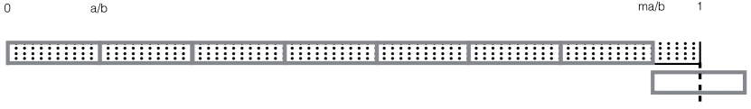
Figure 8: In this example $1-\kappa=a/b=11/83$, the number of full rectangles that can be fit in the line of length 1 is $m=7$ and $c_{m}=1-m(1-\kappa)=(83-77)/83=6/83.$

Proceeding as in parts $(i)$ and $(ii)$ we have

$$\begin{split}\mathbb{E}\Big{[}X^{(N)}_{1}-x\Big{]}&=\sum_{r=0}^{m}\mathbb{E}\Big{[}X^{(N)}_{1}-x\Big{|}N-C_{(1,\underline{M}_{1}(N))}\in[ra/b,(r+1)a/b)\Big{]}\\ &\hskip 99.58464pt\times\mathbb{P}\Big{(}N-C_{(1,\underline{M}_{1}(N))}\in[ra/b,(r+1)a/b)\Big{)}\\ &=\sum_{r=1}^{m}\mathbb{E}\left[\frac{\sum_{i=1}^{\underline{M}_{1}(N)}(\mathbf{1}_{\{t(1,i)=0\}}-x)+G_{r}(1-x)}{\underline{M}_{1}(N)+G_{r}}\right]c_{r}\\ &=\frac{1-x}{N_{x}}\sum_{r=1}^{m}c_{r}\mathbb{E}\left[G_{r}\frac{N_{x}}{\underline{M}_{1}(N)+G_{r}}\right]\\ &\sim\frac{(1-\kappa x)(1-x)}{N}\sum_{r=1}^{m}c_{r}x\frac{1-x^{r}}{1-x}\\ &=\frac{(1-\kappa x)x}{N}\sum_{r=1}^{m}c_{r}(1-x^{r}).\end{split}$$

To complete the proof, we proceed similarly as in parts $(i)$ and $(ii)$. Again, the SDE (1.7) has a unique strong solution. We denote by $\mathcal{A}$ its infinitesimal generator, whose domain contains $C^{2}([0,1])$. If $f\in C^{2}([0,1])$ and $x\in[0,1]$, the discrete generator of $X^{(N)}$ satisfies

$$\begin{split}A^{N}f(x)&=x(1-x)(1-\kappa x)\sum_{j=1}^{b-1}c_{j}(1-x^{j})f^{\prime}(x)\\ &\hskip 113.81102pt+x(1-x)(1-\kappa x)f^{\prime\prime}(x)+o(1)\\ &\to\mathcal{A}f(x),\end{split}$$

and again, the conclusion follows. ∎

Before proving Proposition 3, we start by proving two other results on the path behavior of the Wright-Fisher diffusion with efficiency under (M2).

Lemma 3.

Let $X=(X_{t},t\geq 0)$ be the unique strong solution of (1.5) parametrised by a rational number $\kappa\in(0,1)$ and $\alpha\geq 0$. The boundary points $0$ and $1$ are accesible.

Proof.

Let $X=(X_{t},t\geq 0)$ be the unique strong solution of (1.5) parametrised by $\alpha\geq 0$ and $\kappa$ a rational number in $(0,1)$. For $c\in\mathbb{R}$, consider the process $\overline{Y}^{(c)}=(\overline{Y}^{{(c)}}_{t},t\geq 0)$ defined in the proof of Lemma 2. Recall that both boundaries 0 and 1 are accessible for this process. Again, we use a stochastic domination argument. If $\alpha>0$, we have, a.s.

$$\overline{Y}^{(\kappa)}_{t}\geq X_{t}\geq\overline{Y}^{(\alpha/(\kappa-1))}_{t},\ t\geq 0,$$

and if $\alpha=0,X\equiv\overline{Y}^{(\kappa)}$, and the conclusion follows. ∎

Proposition 6.

Let $X=(X_{t},t\geq 0)$ be the unique strong solution of (1.5) parametrised by $\alpha\geq 0$ and $\kappa$ a rational number in $(0,1)$. Then

$$\mathbb{E}[T_{0,1}|X_{0}=x]<\infty.$$

Proof.

We follow closely the proof of Proposition 1. Recall that the Wright-Fisher diffusion with efficiency under (M1) or (M2) have the same infinitesimal variance, so the Green’s function associated to the Wright-Fisher diffusion with efficiency under (M2) also satisfies equation (2.11) (where $S$ is its scale function). The conclusion follows by the same arguments that are used to prove item $(ii)$ of Proposition 1. ∎

Proof of Proposition 3.

By the same arguments as in the proof of Proposition 2, we have

$$\mathbb{P}_{y}(\{{\rm Fix.}\})=\mathbb{P}(X_{T_{0,1}}=0|X_{0}=1-y)=\frac{S(1)-S(1-y)}{S(1)-S(0)},$$

where $S$ is the scale function of the Wright-Fisher diffusion with efficiency (M2) , which, for $x\in[0,1]$ is given by

$$S(x) = \int_{0}^{x}\exp\left\{-2\int_{\theta}^{u}\left(\kappa-\frac{\alpha}{1-\kappa v}\right)\mathrm{d}v\right\}\mathrm{d}u$$

$$= K\int_{0}^{x}\exp(-2\kappa u)(1-\kappa u)^{-2\alpha/\kappa})\mathrm{d}u,$$

where $\theta$ is an arbitrary positive number and $K$ is a constant that depends on $(\kappa,\alpha,\theta)$. ∎

Acknowledgements. All authors would like to thank Ximena Escalera, José Carlos Ramón Hernández and Fernanda López for carefully reading a preliminary version of this paper and for many useful discussions. We want to thank as well the two anonymous referees whose careful reading led to significant improvements.

JCP acknowledges support from the Royal Society and CONACyT (CB-250590). This work was concluded whilst JCP was on sabbatical leave holding a David Parkin Visiting Professorship at the University of Bath, he gratefully acknowledges the kind hospitality of the Department and University. AGC acknowledges support from UNAM (PAPIIT IA100419) and CONACYT (CB-A1-S-14615). VMP acknowledges support from the DGAPA-UNAM postdoctoral program.

References

References

- [Baake et al. (2018)] Baake, E, González Casanova, A., Probst, S. and Wakolbinger, A. (2019) Modelling and simulating Lenski’s long-term evolution experiment. Theor. Pop. Biol. 127, 58–74.
- [Beardmore et al. (2011)] Beardmore, R. E., Gudelj, I., Lipson, D. A., and Hurst, L. D. (2011). Metabolic trade-offs and the maintenance of the fittest and the flattest. Nature 472, 342-346.
- [Brisson (2018)] Brisson, D. (2011). Negative Frequency-Dependent Selection Is Frequently Confounding. Frontiers in Ecology and Evolution, 6, 10.
- [Donnelly and Weber (1985)] Donnelly, P. and Weber, N. (1985). The Wright-Fisher model with temporally varying selection and population size. Journal of Mathematical Biology, 22, 1, 21–29.
- [Etheridge (2011)] Etheridge, A. (2011) Some mathematical models from population genetics. Some mathematical models from population genetics. École d’Été de Probabilités de Saint-Flour XXXIX-2009. Lecture Notes in Mathematics. Springer
- [Ethier and Kurtz (1986)] Ethier, S.N., Kurtz, T.G. (1986) Markov processes. Characterization and convergence. Wiley Series in Probability and Mathematical Statistics: Probability and Mathematical Statistics. John Wiley & Sons, Inc., New York.
- [Ewens (1963)] Ewens, W.J. (1963) The mean time for absorption in a process of genetic type. J. Australian Math. Soc., 3, 375–383.
- [Fisher (1958)] Fisher, R.A. (1958) The Genetical Theory of Natural Selection. Dover, New York.
- [Fitzpatrick et al. (2007)] Fitzpatrick, M. J., Feder, E., Rowe, L., and Sokolowski, M. B. (2007). Maintaining a behaviour polymorphism by frequency-dependent selection on a single gene. Nature 447, 210–212.
- [González Casanova et al.(2017)] González Casanova, A., Pardo, J.C., Pérez, J.L. (2017) Branching processes with interactions: the subcritical cooperative regime. Preprint Arxiv:1704.04203
- [González Casanova et al. (2016)] González Casanova, A., Kurt, N., Wakolbinger, A., Yuan, L. (2016) An individual-based model for the Lenski experiment, and the deceleration of the relative fitness. Stochastic Process. Appl., 126, 2211–2252.
- [González Casanova and Spano (2018)] González Casanova, A., Spanó, D. (2018) Duality and Fixation in a -Wright-Fisher processes with frequency-dependent selection. Ann. Appl. Probab., 28, 250–284.
- [Griffiths and Tavaré (1994)] R.C. Griffiths and S. Tavaré. (1994) Sampling theory for neutral alleles in a varying environment. Philos. Trans. Royal Soc. B, 344, 403–410.
- [Hairer (2016)] Hairer, M. (2016) Lecture notes on the convergence of Markov processes. Available at: http://www.hairer.org/notes/Convergence.pdf
- [Harris (1952)] Harris, T.E. (1952) First passage and recurrence distributions. Trans. Amer. Math. Soc., 73, 471–486.
- [Jagers and Sagitov (2004)] P. Jagers and S. Sagitov. (2004) Convergence to the coalescent in populations of substantially varying size. J. Appl. Probab., 41, 368–378.
- [Jensen and Kurt (2014)] Jansen, S., and Kurt, N. (2014) On the notion(s) of duality for Markov processes. Probab. Surv., 11, 59–120.
- [Kallemberg (1997)] Kallenberg, O. (1997) Foundations of modern probability. Probability and its Applications. Springer-Verlag, New York.
- [Kaj and Krone (2003)] Kaj, I., Krone, S.M. (2003) The coalescent process in a population of stochastically varying size. J. Appl. Probab., 40, 33–48.
- [Kluth and Baake (2013)] Kluth, S., and Baake, E. (2013) The Moran model with selection: Fixation probabilities, ancestral lines, and an alternative particle representation. Theor. Popul. Biol., 90, 0, 104–112
- [Krone and Neuhauser (1997a)] Krone, S.M. and Neuhauser, C. (1997) The genealogy of samples in models with selection. Genetics, 145 , 519–534.
- [Krone and Neuhauser (1997b)] Krone, S.M. and Neuhauser, C. (1997) Ancestral processes with selection. Theor. Popul. Biol., 51, 210–237.
- [Lambert (2005)] Lambert, A. (2005) The branching process with logistic growth, Ann. App. Probab., 15, 1506–1535.
- [Lamperti (1960)] Lamperti, J. (1960) Criteria for the recurrence or transience of stochastic processes. I. J. Math. Anal. Appl., 1, 314–330.
- [Lenski (n.d.)] Lenski, R.E. E. coli long-term experimental evolution project site. Available at: http://lenski.mmg.msu.edu/ecoli/index.html
- [Lenski and Travisano (1994)] Lenski, R.E., Travisano, M. (1994) Dynamics of adaptation and diversification: a 10,000-generation experiment with bacterial populations. Proc. Natl. Acad. Sci. USA, 91, 15, 6808–6814.
- [Lenz et al. (2015)] Lenz, U., Kluth, S., Baake, E., and Wakolbinger, A. (2015) Looking down in the ancestral selection graph: A probabilistic approach to the common ancestor type distribution. Theor. Popul. Biol.. 103, 27–37.
- [Lipson (2015)] Lipson, D.A. (2015) The complex relationship between microbial growth rate and yield and its implications for ecosystem processes. Frontiers in Microbiology 6, 615.
- [MacArthur and Wilson (1967)] MacArthur, R, and Wilson, E.O. (1967) The theory of island biogeography. Princeton University Press.
- [Mano (2009)] Mano, S. (2009) Duality, ancestral and diffusion processes in models with selection. Theor. Popul. Biol., 75, 2-3, 164–175.
- [Miller et al. (2005)] Miller, T.E., Burns, J.H., Munguia, P., Walters, E.L., Kneitel, J.M., Richards, P.M., Mouquet, N., Buckley, H.L. (2005) A critical review of twenty years’ use of the resource-ratio theory. Am. Nat., 165, 4, 439–448.
- [Molenaar et al. (2009)] Molenaar, D., Van Berlo, R., De Ridder, D., and Teusink, B. (2009). Shifts in growth strategies reflect tradeoffs in cellular economics. Mol. Syst. Biol. 5 323.
- [Norris (1998)] Norris, J.R. (1998) Markov chains. Cambridge Series in Statistical and Probabilistic Mathematics. Cambridge University Press, Cambridge.
- [Novak et al. (2006)] Novak, M., Pfeiffer, T. , Lenski, R.E., Sauer, U, and Bonhoeffer, S. (2006) Experimental Tests for an Evolutionary Trade-off between Growth Rate and Yield in E. coli.. The American Naturalist 168 , 2, 242–251.
- [Parsons et al. (2007a)] Parsons, T. L. and Quince, C. (2007) Fixation in haploid populations exhibiting density dependence I: The non-neutral case. Theor. Pop. Biol., 72(1): 121–135.
- [Parsons et al. (2007b)] Parsons, T. L. and Quince, C. (2007) Fixation in haploid populations exhibiting density dependence II: The quasi-neutral case. Theor. Pop. Biol., 72(4): 468–479.
- [Parsons et al. (2008)] Parsons, T. L., Quince, C. and Plotkin, J.B. (2008) Absorption and fixation times for neutral and quasi-neutral populations with density dependence. Theor. Pop. Biol., 74(4): 302–310.
- [Parsons et al. (2010)] Parsons, T.L., Quince, C., and Plotkin, J.B. (2010) Some consequences of demographic stochasticity in population genetics. Genetics, 185, 4, 1345–1354.
- [Pianka (1970)] Pianka, E.R. (1970) On r and K selection. American Naturalist, 104(940), 592–597.
- [Seneta (1974)] Seneta, E. (1974) A note on the balance between random sampling and population size. Genetics, 77, 3, 607–610.
- [Tilman (1982)] Tilman, A. (1982) Resource Competition and Community Structure. Princeton University Press.
- [Turelli and Barton (2004)] Turelli M. and Barton N.H. (2004) Polygenic variation maintained by balancing selection: Pleiotropy, sex-dependent allelic effects and G x E interactions. Genetics 166, 1053–1079.
- [Wright (1931)] Wright, S. (1931) Evolution in Mendelian Population Genetics. Genetics, 16, 2, 97–159.