Non-Markov Enhancement of Maximum Power for Quantum Thermal Machines

Abstract

In this work we study how the non-Markovian character of the dynamics can affect the thermodynamic performance of a quantum thermal engine, by analysing the maximum power output of Carnot and Otto cycles departing from the quasi-static and infinite-time-thermalization regime respectively, introducing techniques for their control optimization in general dynamical models. In our model, non-Markovianity is introduced by allowing some degrees of freedom of the reservoirs to be taken into account explicitly and share correlations with the engine by Hamiltonian coupling. It is found that the non-Markovian effects can fasten the control and improve the power output.

I Introduction

Quantum Thermodynamics Gemmer et al. (2009); Goold et al. (2016); Vinjanampathy and Anders (2016) was born and rapidly grew in the last decades. Fuelled by high experimental control of quantum systems and engineering at microscopic scales, one of the central goals of physicists is to push the limits of conventional thermodynamics, and the extension of standard models and cycles to include quantum effects and small ensemble sizes. Beyond the drive to clarify fundamental physical issues, these models may also turn out to be relevant from a more practical point of view: it is expected that industrial need for miniaturisation of technologies will benefit from the understanding of quantum thermodynamic processes. In both biology, for example, and nanotechnology, where the benefits from a cooling at the atomic scales are clear, refrigerators models Linden et al. (2010); Skrzypczyk et al. (2011) based on quantum thermal machines could find actual application. Moreover, proposals for experimental realisations of quantum engines were made considering various physical platforms, and many were actually realised Koski et al. (2014); Pekola (2015); Batalhão et al. (2014); An et al. (2015); Roßnagel et al. (2016); Zhang et al. (2014a); Abah et al. (2012); Ronzani et al. (2018); Chen (1994); Rezek and Kosloff (2006); Watanabe et al. (2017); Scully et al. (2011); Correa et al. (2013); Dorfman et al. (2013); Brunner et al. (2014); Zhang et al. (2014a); Campisi and Fazio (2016); Brandner et al. (2017).

Thermodynamics is, par excellence, a theory involving non-isolated systems, and it must take into account the interaction and evolution induced by external degrees of freedom on a working medium. The description of open quantum systems Breuer and Petruccione (2002) needs however, especially in cases where the number of degrees of freedom of the surroundings is big, an effective description on the local degrees of freedom by means of some approximation or assumption. The most important class of simplified dynamics of open systems goes under the name of Markovian dynamics. From the physical point of view, Markovianity is associated to systems interacting with large, unperturbed environments that “spread away the information” contained in the system, while on the formal side different definitions of quantum Markovianity Rivas et al. (2014); Breuer et al. (2016) were introduced in the literature. We stand by the approach (although the model we will consider is non-Markovian even for stronger definitions of quantum Markovianity Rivas et al. (2014); Breuer et al. (2016)) which identifies the Markovian character of a quantum process with its CP-divisibility Rivas et al. (2010) hence admitting a first order Master Equation (ME) that can be casted in the Gorini-Kossakowski-Sudarshan-Lindblad form (GKSL) Gorini et al. (1976); Lindblad (1976).

Recent works have started to investigate how the breaking of the Markovianity in quantum dynamics can affect control and performance of quantum thermodynamic systems, motivated both by the necessity to overcome the approximation on very small systems, and by the speculation of non-Markovianity possibly being an actual resource in practical tasks, see e.g. Refs. Bhattacharya et al. (2018); Bylicka et al. (2016); Mirkin et al. (2017); Mukherjee et al. (2015); Raja et al. (2018); Reich et al. (2015); Thomas et al. (2018); Zhang et al. (2014b); Basilewitsch et al. (2017); Pezzutto et al. (2018). We contribute here considering two archetypical classes of thermal engines, i.e. the quantum Carnot cycle and the quantum Otto cycle Quan et al. (2007); Karimi and Pekola (2016); Kosloff and Rezek (2017); Watanabe et al. (2017); Rezek and Kosloff (2006); Abah et al. (2012) which use as working medium a two-level (qubit) system coupled to two thermal reservoirs while being externally driven. For these models we simulate non-Markovian effects by splitting the degrees of freedom of the system environmental baths into a local contribution, which we treat dynamically, and a remote component which instead is described in terms of an effective GKSL Master Equation that tends to drive the rest of the model into thermal equilibrium. In this configuration it can be shown that the coupling with the local bath components ignites the non-Markovian behaviour of the model whose effects can then be tested in terms of the engine performance. In particular, performing an optimization on the external driving, we show that, both in the Carnot and Otto scheme, the maximum power extractable improves with respect to the Markovian limit. To do this we first discuss both cycles in the finite-time regime; to solve the dynamics and optimize the control for the Carnot cycle, we use the powerful technique introduced in Cavina et al. (2017a) (Slow-Driving approximation, or S-D), which efficiently solves the approximate dynamics of a system slowly perturbed from thermalization. For the Otto case we use exact solutions.

The article is structured as follows:
Sec. II and Sec. III are devoted to introduce the technical tools we use to derive the results of Sec. IV. Specifically in Sec. II we discuss the physics of an externally controlled, quantum thermal machine introducing the notation in Sec. II.1, drawing general thermodynamic considerations in Sec. II.2 and reviewing some basic facts about the S-D approximation method Cavina et al. (2017a) in Sec. II.3. In Sec. III instead we analyze the performances of some thermodynamic cycles. In particular Sec. III.1 is devoted to study the quantum Carnot cycle in the quasi-static approximation and its first order S-D corrections, recovering some known results in a slightly broader context. Sec. III.2 instead focuses on the Otto cycle. In Sec. IV we finally introduce the specific non-Markovian model. Using the preceding section results, we then show how the power output of the cycles gets affected both for the Carnot machine (Sec. IV.2) and for the Otto machine (Sec. IV.3). In Sec. IV.4 an argument is presented to interpret the results obtained, focusing on why the information flow induced by non-Markovianity can fasten the speed of thermalization. Comments and conclusions are presented in Sec. V while the Appendix contains some technical derivations.

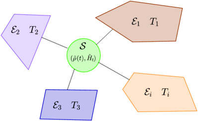
Figure 1: General schematics of a quantum thermal machine with working medium described by the quantum system $\mathcal{S}$, characterized by local Hamiltonian ${\hat{H}_{t}}$, connected with different thermal baths $\mathcal{E}_{i}$, described by temperatures $T_{i}$ and coupled with ${\cal S}$.

II Quantum thermal machines in the Markovian regime

In this section we review some basic facts about quantum thermal machines in the Markovian regime, setting the notation and developing the tools that we shall later employ for analysing the non-Markovian case.

II.1 The setup

Consider a quantum working medium ${\cal S}$ characterized by a time-dependent internal Hamiltonian $\hat{H}_{t}$ which can be externally controlled via some classical pulses. As schematically shown in Fig. 1 ${\cal S}$ is coupled to a collection of external thermal baths $\{{\cal E}_{j}\}$ characterized by temperatures $T_{j}$, which are also externally controlled to allow selective activation and deactivation. In particular we shall assume at each time $t$ only one of the baths is actively coupled with the working medium. Accordingly, enforcing the Markovian character in the system-bath interactions, we describe the evolution of ${\cal S}$ in terms of a Master Equation Breuer and Petruccione (2002) associated with a step-continuous generator ${\cal L}_{t}$ which, on the time interval ${\cal I}_{j}$ where only the $j$-th bath interaction is active, writes

$$\dot{\hat{\rho}}(t)={\cal L}_{t}[\hat{\rho}(t)]:=-i[\hat{H}_{t},\hat{\rho}(t)]_{-}+\mathcal{D}_{t}^{(j)}[\hat{\rho}(t)]\ ,$$ (1)

where $\hat{\rho}(t)$ is the density matrix of ${\cal S}$ at time $t$, $[\cdots,\cdots]_{-}$ is the commutator symbol, and where finally $\mathcal{D}_{t}^{(j)}$ is the GKSL dissipator Gorini et al. (1976); Lindblad (1976) mimicking the interaction with ${\cal E}_{j}$ (hereafter for easy of notation we set both the Plank and the Boltzmann constant equal to one, i.e. $\hbar=k_{\rm B}=1$).

As indicated by the notation the $\mathcal{D}_{t}^{(j)}$s exhibit an explicit time dependence which, in a weak-coupling regime, we assume to be a direct consequence of the modulations affecting the system Hamiltonian, i.e.

$$\mathcal{D}_{t}^{(j)}=\mathcal{D}^{(j)}(\hat{H}_{t})\;.$$ (2)

Furthermore, in order to impose proper thermalization conditions on the scheme we require $\mathcal{D}_{t}^{(j)}$ to admit the instantaneous Gibbs state

$$\hat{\Omega}^{(j)}_{\hat{H}_{t}}:=\frac{e^{-\beta_{j}\hat{H}_{t}}}{\text{Tr}[e^{-\beta_{j}\hat{H}_{t}}]}\;,$$ (3)

with $\beta_{j}:=1/T_{j}$ being the associated inverse temperature, as unique fixed point, i.e.

$$\mathcal{D}_{t}^{(j)}[\hat{\rho}]=0\;\;\Leftrightarrow\;\;\hat{\rho}=\hat{\Omega}_{t}^{(j)}\;.$$ (4)

Notice that the functional dependence of $\hat{\Omega}^{(j)}_{\hat{H}_{t}}$ with respect to $\hat{H}_{t}$, ensures that the requirement Eq. (4) is fully compatible with (2) and it implies that for $t\in{\cal I}_{j}$, $\hat{\Omega}^{(j)}_{\hat{H}_{t}}$ is also the unique fixed point of the full generator ${\cal L}_{t}$, i.e.

$$\mathcal{L}_{t}[\hat{\rho}]=0\;\;\Leftrightarrow\;\;\hat{\rho}=\hat{\Omega}^{(j)}_{\hat{H}_{t}}\;.$$ (5)

Explicit examples of dissipators $\mathcal{D}_{t}^{(j)}$ obeying the above constraints are presented in Appendix A, here we only remark that they have been extensively used in the characterization of equilibration processes induced by fermionic or bosonic baths, see e.g. Refs. Cavina et al. (2017b); Gardiner et al. (2004); Breuer and Petruccione (2002); Esposito et al. (2010). In the absence of Hamiltonian modulations (i.e. for $\hat{H}_{t}=\hat{H}$ constant), Eqs. (4) and (5) ensure that if ${\cal S}$ is left in contact with the $j$-th bath, it will be forced by (1) to asymptotically reach thermal equilibrium at temperature $T_{j}$, i.e.

$$\lim_{t\rightarrow\infty}\hat{\rho}(t)=\hat{\Omega}^{(j)}_{\hat{H}}\;,$$ (6)

irrespectively from the initial condition of the problem.

II.2 Energy exchanges and thermodynamic consistency

Within the above theoretical framework the internal energy $E(t)$ of ${\cal S}$ can be identified with the expectation value of $\hat{H}_{t}$ on $\hat{\rho}(t)$, i.e.

$$E(t):=\text{Tr}[\hat{\rho}(t)\hat{H}_{t}]\ .$$ (7)

Its infinitesimal variation comprises two terms which, following the canonical approach of Refs. Alicki (1979); Anders and Giovannetti (2013); Kieu (2004); Vinjanampathy and Anders (2016), are associated respectively with a work (performed on ${\cal S}$) contribution

$$dW(t):=\text{Tr}[\hat{\rho}(t)d\hat{H}_{t}]\ ,$$ (8)

and with a heat (absorbed by ${\cal S}$) contribution

$$dQ_{j}(t) := \text{Tr}\Big{[}\hat{H}_{t}d\hat{\rho}(t)\Big{]}$$ (9)

$$= \text{Tr}\Big{[}\hat{H}_{t}\mathcal{D}_{t}^{(j)}[\hat{\rho}(t)]\Big{]}\;dt\;,$$ (10)

where in the second identity we make explicit use of Eq. (1), ${\cal E}_{j}$ being the only bath that is coupled with ${\cal S}$ at time $t$. It is worth stressing that the consistency of the above identifications is explicitly justified by the Markovian character of the thermalizing process we are considering. To see this let us introduce the functional Parrondo et al. (2015); Esposito and den Broeck (2011)

$$F(\hat{\rho}(t),\hat{H}_{t}):=E(t)-S(\hat{\rho}(t))/\beta_{j}\;,$$ (11)

where $S(\hat{\rho}(t)):=-\mbox{Tr}[\hat{\rho}(t)\ln\hat{\rho}(t)]$ is the von Neumann entropy of $\hat{\rho}(t)$. Exploiting the formal connection between informational and thermodynamical entropy, the quantity (11) can be identified with the counterpart of the free energy functional of classical equilibrium thermodynamics. One can easily verify that it obeys the identity

$$F(\hat{\rho}(t),\hat{H}_{t})-F(\hat{\Omega}^{(j)}_{\hat{H}_{t}},\hat{H}_{t})=S(\hat{\rho}(t)\parallel\hat{\Omega}^{(j)}_{\hat{H}_{t}})/\beta_{j}\;,$$ (12)

where $S(\hat{\rho}_{1}\parallel\hat{\rho}_{2}):=-S(\hat{\rho}_{1})-\mbox{Tr}[\hat{\rho}_{1}\ln\hat{\rho}_{2}]$ is the relative entropy functional Holevo (2012). The latter is know to be decreasing when the same completely positive mapping acts on both its argument: accordingly, given that the dynamical generator ${\cal L}_{t}$ of Eq. (1) is guaranteed to grant complete positive evolution and using the invariance (5) of $\hat{\Omega}^{(j)}_{\hat{H}_{t}}$ we can claim that $S({\cal L}_{t}[\hat{\rho}(t)]\parallel\hat{\Omega}^{(j)}_{\hat{H}_{t}})\leq 0$. Inserting this into (12) we can establish that the time derivative of the l.h.s. must be upper bounded by the quantity $S(\hat{\rho}(t)\parallel\frac{d}{dt}\hat{\Omega}^{(j)}_{\hat{H}_{t}})/\beta_{j}$, which after proper reordering of the various terms leads to the inequality

$$dF(\hat{\rho}(t),\hat{H}_{t})\leq dW(t)\Longleftrightarrow\beta_{j}dQ_{j}(t)\leq dS(\hat{\rho}(t))\;,$$ (13)

that is an instance of the 2nd Law of thermodynamics providing an operational justification for the definitions (8) and (9).

II.3 Thermodynamic cycles

Integrating Eq. (1) we can now analyze the work production rates, their associated efficiencies, and the corresponding heat fluxes, of thermodynamic cycles where the system ${\cal S}$ is externally driven by an assigned modulation of the Hamiltonian $\hat{H}_{t}$ while being put in selective contact with the baths ${\cal E}_{j}$s – see below. Unfortunately the presence of Hamiltonian modulations makes typically Eq. (1) hard to solve. Yet assuming the time scale at which (6) takes places to be short enough, one expects ${\cal S}$ to have enough time to adiabatically follow the instantaneous fixed points of Eq. (3), obtaining

$$\hat{\rho}(t)\simeq\hat{\Omega}^{(j)}_{\hat{H}_{t}}\;.$$ (14)

This is the standard quasi-static regime where the working medium is always at thermal equilibrium with one of the baths. Departing from this scenario one enters the regime of Finite Time Thermodynamics (FTT) Andresen et al. (1984), where the time-scales on which the external controls responsible for the modulations of $\hat{H}_{t}$ occur, begin to compete with the thermalization times. In what follows we shall study this complex regime by adopting the Slow-Driving (S-D) approximation technique introduced in Ref. Cavina et al. (2017a). The latter is a perturbative approach which can be applied to study deviations from Eq. (14) in the limit of slow variation of $\mathcal{L}_{t}$. As we detail in Appendix B, the S-D approximation can be used as a way for putting on firm ground some of the assumptions typically adopted in FFT analysis. It accounts in expressing the solution of Eq. (1) as an expansion series with a perturbation parameter given by the ratio $\tau_{R}/\tau$ between the typical timescale $\tau\sim\|\dot{\mathcal{L}}_{t}/\mathcal{L}_{t}\|$ associated with the variation of the dynamics generator, and the typical relaxation time $\tau_{R}$ governing the convergence of the limit (6). At the lowest orders one has

$$\hat{\rho}(t)=\hat{\rho}^{(0)}(t)+\hat{\rho}^{(1)}(t)+...\;,$$ (15)

with $\hat{\rho}^{(0)}(t):=\hat{\Omega}^{(j)}_{\hat{H}_{t}}$ being the zero-th order term, while the first order correction $\hat{\rho}^{(1)}(t)$ is obtained as Cavina et al. (2017a)

$$\hat{\rho}^{(1)}(t)=(\mathcal{L}_{t}\mathcal{P})^{-1}[\dot{\hat{\rho}}^{(0)}(t)]\,,$$ (16)

where $\mathcal{P}$ is the projector on the null-trace subspace of linear operators (its presence being required to make $\mathcal{L}_{t}$ invertible, under the assumption of unique null eigenstate). Therefore, by direct substitution in Eq. (10) we get

$$dQ_{j}(t)\simeq dQ_{j}^{(0)}(t)+dQ_{j}^{(1)}(t)\;,$$ (17)

where

$$dQ_{j}^{(0)}(t):=\text{Tr}\Big{[}\hat{H}_{t}d\hat{\rho}^{(0)}(t)\Big{]}=dS^{(0)}(t)/\beta_{j}\;,$$ (18)

is the quasi-static contribution which, by using the fact that $\hat{\rho}^{(0)}(t)$ is the Gibbs state $\hat{\Omega}^{(j)}_{\hat{H}_{t}}$, we expressed in terms of the infinitesimal increment the von Neumann entropy $S^{(0)}(t):=-\mbox{Tr}[\hat{\rho}^{(0)}(t)\ln\hat{\rho}^{(0)}(t)]$ of the latter, and where

$$dQ_{j}^{(1)}(t)=\text{Tr}\Big{[}\hat{H}_{t}d\hat{\rho}^{(1)}(t)\Big{]}\;,$$ (19)

is the first order correction term.

III Thermodynamic cycles optimisation

In this section we will show how it is possible to optimize the control on a quantum engine in order to maximize is performance, i.e. its power output, addressing the paradigmatic case of Quantum Carnot and Otto cycles performed on a two-level (qubit) system ${\cal S}$ which evolves under the influence of a hot bath H and a cold bath C, the modulation of its Hamiltonian being associated with control pulses that act on its energy gap $\epsilon(t)\geq 0$, i.e.

$$\hat{H}_{t}={\epsilon}(t)\hat{\mathcal{\sigma}}^{z}/2\ ,$$ (20)

with $\hat{\mathcal{\sigma}}^{z}$ being the third Pauli matrix, with eigenstates $|0\rangle$ and $|1\rangle$. It’s not difficult to generalise these cycles (in the quasi-static regime) to more general Hamiltonians. While in deriving the above considerations we shall make explicit reference to the expressions we developed in Sec. II for the Markovian regime, we stress that the results we obtain also hold for non-Markovian dynamics, as we shall use them later in Sec. IV to analyse the non-Markovian model we present.

III.1 Quantum Carnot Cycle

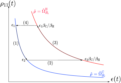
Figure 2: (Color online) Pictorial representation of the (quasi-static) Quantum Carnot cycle in the configuration space $\rho_{11}(t):=\langle 1|\hat{\rho}(t)|1\rangle$ vs. the energy gap $\epsilon(t)$ in the ideal quasi-static limit. Steps 1) and 3) correspond to the isothermal transformations where ${\cal S}$ is kept in contact with the cold bath $\rm C$ and hot bath $\rm H$, respectively; steps 2) and 4) instead represent sudden quenches of the Hamiltonian gap.

A Quantum Carnot cycle is identified with a 4 steps process inspired directly by its classical counterpart, that is two isothermal strokes where the Hamiltonian of ${\cal S}$ is modulated while keeping the system in thermal contact with one of the two baths, alternated with two iso-entropic (adiabatic) strokes, where instead the Hamiltonian undergoes to instantaneous sudden switches (quenches). In the ideal quasi-static limit (14) the operations are performed slowly enough to allow the system to be in thermal equilibrium at every instant, i.e. states which for the Hamiltonian (20) can be expressed as

$$\hat{\Omega}^{({j})}_{\hat{H}_{t}}=\hat{\Omega}^{({j})}_{\epsilon(t)}:=p_{j}(\epsilon(t))|0\rangle\langle 0|+(1-p_{j}(\epsilon(t)))|1\rangle\langle 1|\;,$$ (21)

with

$$p_{j}(\epsilon):=\dfrac{1}{1+e^{-\beta_{j}\epsilon}}\;,$$ (22)

being the associated ground state population.

In this case the 4 steps of the cycle are as in Figure 2:

• while being coupled to the cold reservoir C, the energy gap is modified continuously and monotonically, from the initial value $\epsilon_{1}$ to $\epsilon_{2}\geq\epsilon_{1}$ (more precisely we require $\epsilon(t)$ to be continuous and differentiable with first order derivative which is not negative);

• with the system isolated from the reservoirs, a quench is now performed by suddenly taking the gap from $\epsilon_{2}$ to

  $$\epsilon_{3}:=\epsilon_{2}{\beta_{\rm C}}/{\beta_{\rm H}}\;,$$ (23)

  which by construction is larger than $\epsilon_{2}$, i.e. $\epsilon_{3}\geq\epsilon_{2}$;

• while being coupled to the hot reservoir H, the energy gap is then modified continuously, and monotonically, from $\epsilon_{3}$ to

  $$\epsilon_{4}:=\epsilon_{1}{\beta_{\rm C}}/{\beta_{\rm H}}\;,$$ (24)

  that automatically fulfils the constraint $\epsilon_{1}\leq\epsilon_{4}\leq\epsilon_{2}{\beta_{\rm C}}/{\beta_{\rm H}}=\epsilon_{3}$ (again, more precisely we require $\epsilon(t)$ to be continuous and differentiable with first order derivative that is non-positive);

• finally isolating the system a quench is performed to restore the gap at the initial value $\epsilon_{1}$.

It is worth pointing out that the continuity requirement of $\epsilon(t)$ during the steps 1) and 3) is inserted in order to make sure that one could later on apply the S-D expansion which needs to have a zero-th order contribution of term differentiable – see Eq. (15). More specifically in what follows we shall require $\epsilon(t)$ to have null first order derivative at the extrema of the isotherms. This is a technical assumption which we introduce in order to ensure the solution of the dynamics (15) to be continuous and differentiable also in proximity of the quenches (where it coincides with the Gibbs state (21)), which in turn implies that no first order correction (16) at the extremal points of the isothermal strokes has to be expected. The monotonicity behaviour of $\epsilon(t)$ during the steps 1) and 3) is instead motivated by energetic considerations. As a matter of fact having set the gap to evolve monotonically from $\epsilon_{1}\geq 0$ to $\epsilon_{2}\geq\epsilon_{1}$, we can ensure that at each instant of step 1) the system always releases heat to the cold bath without absorbing it: this can be easily verified by observing that the von Neumann entropy of a Gibbs state (21) writes

$$S(\hat{\Omega}^{({j})}_{\epsilon})=-p_{j}(\epsilon)\ln p_{j}(\epsilon)-(1-p_{j}(\epsilon))\ln(1-p_{j}(\epsilon))\;,$$ (25)

which is monotonically decreasing with $\epsilon$, and from the fact that at the lowest order in the expansion (18) the associated incremental heat can be expressed as

$$dQ_{\rm C}(t)\simeq dQ^{(0)}_{\rm C}(t) = \frac{dS(\hat{\Omega}^{({\rm C})}_{\epsilon(t)})}{\beta_{\rm C}}\leq 0\;,\quad\forall t\in{\cal I}_{\rm C}\;.$$ (26)

Similarly having ensured that in step 3) the value of the gap decreases monotonically from $\epsilon_{3}$ to $\epsilon_{4}\geq\epsilon_{3}$, we can guarantee that the heat in the process is always absorbed from the bath H, i.e.

$$dQ_{\rm H}(t)\simeq dQ^{(0)}_{\rm H}(t) = \frac{dS(\hat{\Omega}^{({\rm H})}_{\epsilon(t)})}{\beta_{\rm H}}\geq 0\;,\quad\forall t\in{\cal I}_{\rm H}\;.$$ (27)

Thanks to these properties, and by the observation that of course no heat is exchanged between ${\cal S}$ and the baths during the steps 2) and 4), the total heat absorbed by the working medium in a cycle can be obtained by integrating (27) over the full duration of step 3), i.e.

$$Q_{\rm ABS} = \int_{{\cal I}_{\rm H}}dQ_{\rm H}(t)$$

$$\simeq \int_{{\cal I}_{\rm H}}dQ^{(0)}_{\rm H}(t)=\frac{S(\hat{\Omega}^{({\rm H})}_{\epsilon_{4}})-S(\hat{\Omega}^{({\rm H})}_{\epsilon_{3}})}{\beta_{\rm H}}\geq 0\;,$$

while the total released heat is given by

$$Q_{\rm REL} = \int_{{\cal I}_{\rm C}}dQ_{\rm C}(t)$$

$$\simeq \int_{{\cal I}_{\rm C}}dQ^{(0)}_{\rm C}(t)=\frac{S(\hat{\Omega}^{({\rm H})}_{\epsilon_{2}})-S(\hat{\Omega}^{({\rm H})}_{\epsilon_{1}})}{\beta_{\rm C}}\leq 0\;.$$

Notice also that the constraints (23) and (24) impose

$$p_{\rm H}(\epsilon_{3})=p_{\rm C}(\epsilon_{2})\;\qquad p_{\rm H}(\epsilon_{4})=p_{\rm C}(\epsilon_{1})\;,$$ (30)

which implies $\hat{\Omega}^{({\rm H})}_{\epsilon_{3}}=\hat{\Omega}^{({\rm C})}_{\epsilon_{2}}$ and $\hat{\Omega}^{({\rm H})}_{\epsilon_{4}}=\hat{\Omega}^{({\rm C})}_{\epsilon_{1}}$. Accordingly by direct inspection of (III.1) and (III.1) we obtain the fundamental identity

$$\Delta Q^{(0)}_{\rm H}=-\frac{\beta_{C}}{\beta_{H}}\Delta Q^{(0)}_{\rm C}\;,$$ (31)

which we expressed in terms of the simplified notation $\Delta Q^{(0)}_{j}:=\int_{{\cal I}_{j}}dQ^{(0)}_{j}(t)$. Now, since the work produced by ${\cal S}$ on a cycle can be identified with $Q_{\rm ABS}+Q_{\rm REL}$ by invoking the internal energy conservation, the efficiency (work done over heat absorbed) of the process can be shown to correspond to the Carnot efficiency $\eta_{\text{c}}:=1-\frac{\beta_{\rm H}}{\beta_{\rm C}}$. Indeed

$${\eta}:=\frac{Q_{\rm ABS}+Q_{\rm REL}}{Q_{\rm ABS}}\simeq 1+\frac{\Delta Q^{(0)}_{\rm C}}{\Delta Q^{(0)}_{\rm H}}=\eta_{\text{c}}\;,$$ (32)

the last identity following directly from (31). It is worth stressing that Eqs. (26) and (32) are universal results that do not depend on the specific structure of the generators $\mathcal{D}_{t}^{(j)}$ entering the system ME. This is a consequence of the quasi-static approximation (14) in which, as in classical thermodynamics, complete thermalization is allowed at any time in contact with a thermal source: in this regime no explicit dynamics as in Eq. (1) is needed to describe the thermodynamics of the engine, neither the exact temporal dependence of the control $\epsilon(t)$, except the properties of the equilibrium state (3) and the knowledge of the Hamiltonian at the turning points of the protocol. All this of course holds true as long as we can neglect the first-order contributions in the S-D expansion (15). To account for them we now use (17) to refine Eqs (III.1) and (III.1), writing $Q_{\rm REL}\simeq\Delta Q^{(0)}_{\rm C}+\Delta Q^{(1)}_{\rm C}$ and $Q_{\rm ABS}\simeq\Delta Q^{(0)}_{\rm H}+\Delta Q^{(1)}_{\rm H}$ with

$$\Delta Q^{(1)}_{j}:=\int_{{\cal I}_{j}}dQ^{(1)}_{j}(t)\;,$$ (33)

obtaining

$${\eta} = 1+\frac{Q_{\rm REL}}{Q_{\rm ABS}}\simeq 1+\frac{\Delta Q^{(0)}_{\rm C}}{\Delta Q^{(0)}_{\rm H}}\frac{1+\Delta Q^{(1)}_{\rm C}/\Delta Q^{(0)}_{\rm C}}{1+\Delta Q^{(1)}_{\rm H}/\Delta Q^{(0)}_{\rm H}}$$ (34)

$$= 1-(1-\eta_{\text{c}})\frac{1+\alpha_{\rm C}}{1+\alpha_{\rm H}}\;,$$

where in the last identity we employed (17) to express the ratio $\Delta Q^{(0)}_{\rm C}/\Delta Q^{(0)}_{\rm H}$ in terms of the Carnot efficiency and for $j\in\{{\rm H,C}\}$ introduced the parameter

$$\alpha_{j}:=\Delta Q^{(1)}_{j}/\Delta Q^{(0)}_{j}\;,$$ (35)

to gauge the ratio between the first and the zero-th order heat contributions associated with the $j$-th bath. In a similar fashion we can also express the power $P$ associated with the work production per cycle. Indicating hence with $\tau_{\rm H}$ and $\tau_{\rm C}$ the durations of the transformations 1) and 3) (the only being time-consuming given that step 2) and 4) are assumed to be instantaneous), we write

$$P := \frac{{Q_{\rm ABS}}+{Q_{\rm REL}}}{\tau_{\rm C}+\tau_{\rm H}}\simeq\frac{{\Delta Q^{(0)}_{\rm C}}+{\Delta Q^{(0)}_{\rm H}}+{\Delta Q^{(1)}_{\rm C}}+{\Delta Q^{(1)}_{\rm H}}}{\tau_{\rm C}+\tau_{\rm H}}$$ (36)

$$= {\Delta Q^{(0)}_{\rm H}}\frac{\eta_{\text{c}}+\alpha_{\rm H}-(\beta_{\rm H}/\beta_{\rm C})\alpha_{\rm C}}{\tau_{\rm C}+\tau_{\rm H}}\;,$$

where we used Eqs. (31) and (35).

III.1.1 Performance optimization in the S-D regime

To proceed with our analysis we need to provide some details on the system ME and in particular on the GKSL dissipators which define it. As a preliminary step, however we observe that thanks to our choice (20) we can express Eq. (10) as

$$dQ_{j}(t)=\frac{1}{2}\epsilon(t)[d{\rho}_{11}(t)-d{\rho}_{00}(t)]=-\epsilon(t)d{\rho}_{00}(t)\ ,\ \$$ (37)

where for $k,k^{\prime}=0,1$, ${\rho}_{kk^{\prime}}(t):=\langle k|\hat{\rho}(t)|k^{\prime}\rangle$ are the matrix elements of $\hat{\rho}(t)$ with respect to the eigenbasis of $\hat{H}_{t}$ and where in the second identity we use the normalization condition $\mbox{Tr}[\hat{\rho}(t)]=1$ to write $d{\rho}_{11}(t)=-d{\rho}_{00}(t)$. Due to linearity Eq. (37) applies to all orders of the S-D expansion (17), implying in particular that Eqs. (18), (19) take the form

$$dQ^{(0)}_{j}(t) = -\epsilon(t)d{\rho}^{(0)}_{00}(t)\;,$$

$$dQ^{(1)}_{j}(t) = -\epsilon(t)d{\rho}^{(1)}_{00}(t)\;,$$ (38)

where ${\rho}^{(0)}_{00}(t)$ and ${\rho}^{(1)}_{00}(t)$ are respectively the zero-th and first order contribution to the population of the ground state of ${\cal S}$. The first of these two terms is nothing but the function (22), i.e. ${\rho}^{(0)}_{00}(t)=p_{j}(\epsilon(t))$. The second instead can be determined exploiting Eq. (16). In particular due to the linearity of operators in Eq. (16) and the one-parameter dependence of $\hat{\rho}^{(0)}$ it is possible to draw, in full generality, the following formal connection between ${\rho}^{(1)}_{00}(t)$ and the function $p_{j}(\epsilon(t))$ which, effectively, becomes the real control parameter of the setting. Specifically we get

$${\rho}^{(1)}_{00}(t)=-A_{j}[p_{j}(\epsilon(t))]\;\frac{d}{dt}{p}_{j}(\epsilon(t))\;,$$ (39)

where $A_{j}$, which we dub the S-D amplitude of the problem, quantifies how large is the first order correction determining the relaxation timescale of the setup. In general, besides depending on the the parameters of the model, the S-D amplitude is an explicit functional of ${p}_{j}(\epsilon(t))$, e.g. as in the case of dissipators $\mathcal{D}_{t}^{(j)}$ associated with Bosonic baths defined by Eq. (95) with rates as in (A) for which we get $A_{j}=(2p_{j}(\epsilon(t))-1)/\Gamma_{j}$. When considering instead as dissipators $\mathcal{D}_{t}^{(j)}$ the super-operators defined in Eq. (94) or those associated with fermionic baths defined by Eq. (95) with rates as in (A), one gets an S-D amplitude which is constant, i.e.

$$A_{j}={1}/{\Gamma_{j}}\;,$$ (40)

with $\Gamma_{j}$ being a fundamental constant of the model. In what follows, for the sake of simplicity we shall focus on this special case: our finding however can be approximatively applied to all those configurations where, for all $t\in{\cal I}_{j}$, $A_{j}$ is a slowly varying functional of $p_{j}(\epsilon(t))$.

With the help of the above identities we can hence cast (33) as

$$\Delta Q_{j}^{(1)} = \frac{A_{j}}{\beta_{j}}\int_{{\cal I}_{j}}dt\;\ln\big{(}\tfrac{p_{j}(t)}{1-p_{j}(t)}\big{)}\;\ddot{p}_{j}(t)$$ (41)

$$= -\frac{A_{j}}{\beta_{j}}\int_{{\cal I}_{j}}dt\;\frac{[\dot{p}_{j}(t)]^{2}}{p_{j}(t)(1-p_{j}(t))}\;,$$

where in the first identity we used Eq. (22) to write $\epsilon(t)$ in terms of $p_{j}(t):=p_{j}(\epsilon(t))$, i.e. $\epsilon(t)=\frac{1}{\beta_{j}}\ln\big{(}\tfrac{p_{j}(t)}{1-p_{j}(t)}\big{)}$, and in the second we adopted integration by parts exploiting the fact that at the extrema of the isotherms steps the control functions have been set to have null first order derivative. Equation (41) should be compared with the zero-th order term $\Delta Q_{j}^{(0)}$ which we have already computed in the previous section and which, expressed in terms $p_{j}(t)$, results to be the integral of an exact differential that depends only on the initial and final values $p_{j}^{(in)}$ and $p_{j}^{(fin)}$ assumed on the interval ${\cal I}_{j}$, i.e.

$$\Delta Q_{j}^{(0)} = -\frac{1}{\beta_{j}}\int_{{\cal I}_{j}}dt\;\ln\big{(}\tfrac{p_{j}(t)}{1-p_{j}(t)}\big{)}\;\dot{p}_{j}(t)$$ (42)

$$= -\frac{1}{\beta_{j}}\int_{{\cal I}_{j}}dp\;\ln\big{(}\tfrac{p}{1-p}\big{)}$$

$$= \frac{1}{\beta_{j}}\left(\ln(1-p)+p\ln\frac{p}{1-p}\right)\Big{\rvert}_{p_{j}^{(in)}}^{p_{j}^{(fin)}}\;,$$

the last identity being an alternative way of expressing the entropy increment of the Gibbs state (21).

Our next problem is to determine which choices of $\epsilon(t)$, or equivalently of $p_{j}(t)$, can be used in order to guarantee better performances with respect to the quasi-static regime. To begin with it is worth stressing that from Eq. (41) it follows that for all choices of the control functions the first order correction term to the heat is always negative semi-definite, i.e.

$$\Delta Q_{j}^{(1)}\leq 0\;,$$ (43)

which in turn implies

$$\alpha_{\rm H}\leq 0\;,\qquad\qquad\alpha_{\rm C}\geq 0\;,$$ (44)

due to the positivity of $\Delta Q_{\rm H}^{(0)}$ and the negativity of $\Delta Q_{\rm C}^{(0)}$ (incidentally we observe that  (43) continues to hold by the same argument even if $A_{j}(p_{j})$ is not constant but explicitly dependent on the control $p_{j}(t)$). The first consequence of Eq. (44) is the fact that the efficiency $\eta$ of Eq. (34) cannot be larger than $\eta_{\text{c}}$, as one expects from the second principle of thermodynamics (formally speaking to show that $\eta\leq\eta_{\text{c}}$ we also need $|\alpha_{j}|\ll 1$ which however is always implicit assumed by the perturbative character of the S-D approach). At the level of the power (36) we notice instead that first order corrections explicitly depend on features which one may try to optimize with proper choices of the controls. For this purpose looking at the expression (41) we can isolate different contributions:

• Control speed: keeping the same shape (and extrema) for the driving protocol, we can modify its duration via the mapping $\tau_{j}\rightarrow\lambda\tau_{j}$ with $\lambda>0$. By a simple change of variable $t\rightarrow t/\lambda$ in Eq. (41), it is immediate to find that this induces the following rescaling

  $$\Delta Q_{j}^{(1)}\xrightarrow[t\rightarrow t/\lambda]{}\Delta Q_{j}^{(1)}/\lambda\;,$$ (45)

  while, of course, the zero-order terms $\Delta Q_{j}^{(0)}$ are unaffected;

• Control shape: over a fixed time length, we can clearly optimize with respect to the shape of the function $\epsilon(t)$, i.e. with respect to the function $p_{j}(t)$ under the constraint i), ii) and iii). Once more this will induce a modification of $\Delta Q_{j}^{(1)}$ while leaving unaffected the zero-order contribution terms;

• S-D amplitude selection: this is the main figure of merit after control optimisation. It merely consists in selecting different kind of bath-system interactions in order to influence the value of $\Delta Q_{j}^{(1)}$ via its dependence upon the S-D amplitude $A_{j}$ (this optimization will be specifically analyzed in the study of non-Markovian models).

Let us first analyze how the power $P$ is affected by Speed Control optimization. Using the scaling relations (45) we find that Eq. (36) changes as

$$P\xrightarrow[t\rightarrow t/\lambda_{\rm H,C}]{}{\Delta Q^{(0)}_{\rm H}}\frac{\eta_{\text{c}}-|\alpha_{\rm H}|/\lambda_{\rm H}-(\beta_{\rm H}/\beta_{\rm C})\alpha_{\rm C}/\lambda_{\rm C}}{\tau_{\rm C}\lambda_{\rm C}+\tau_{\rm H}\lambda_{\rm H}}\;,$$ (46)

while the associated efficiency

$$\eta\xrightarrow[t\rightarrow t/\lambda_{\rm H,C}]{}1-(1-\eta_{\text{c}})\frac{1+\alpha_{\rm C}/\lambda_{\rm C}}{1-|\alpha_{\rm H}|/\lambda_{\rm H}}\;,$$ (47)

where we used (44) to rewrite $-\alpha_{\rm H}=|\alpha_{\rm H}|$, and where $\lambda_{\rm C},\lambda_{\rm H}>0$ represent the stretching of the intervals ${\cal I}_{\rm C}$ and ${\cal I}_{\rm H}$, respectively. A simple analytical study reveals that the function (46) admits a maximum for

$$\lambda_{\rm C} =\frac{2\alpha_{\rm C}\beta_{\rm H}}{{\eta}_{\text{c}}\beta_{\rm C}}\bigg{(}1+\sqrt{\frac{|\alpha_{\rm H}|\beta_{\rm C}\tau_{\rm C}}{\alpha_{\rm C}\beta_{\rm H}\tau_{\rm H}}}\bigg{)}\ ,$$ (48)

$$\lambda_{\rm H} =\lambda_{\rm C}\;\frac{\tau_{\rm C}}{\tau_{\rm H}}\;\sqrt{\frac{|\alpha_{\rm H}|\beta_{\rm C}}{\alpha_{\rm C}\beta_{\rm H}}}\ .$$ (49)

Replacing these values into (46) and (47) it is possible then to express the maximum power $P_{\max}$ and the correspondent efficiency at maximum power (EMP) that we indicate with the symbol $\eta^{*}$. For the sake of simplicity let us now suppose $\alpha_{\rm C}=|\alpha_{\rm H}|=\alpha$ and $\tau_{\rm C}=\tau_{\rm H}=\tau$, a regime attained for instance under symmetric bath couplings and driving assumptions, i.e. posing $A_{\rm C}=A_{\rm H}$ and requiring $\epsilon(t)$ during the hot isotherm to be the time-reversal of the cold isotherm – see however Ref. Cavina et al. (2017a) for an explicit treatment of the cases where this hypothesis is relaxed. In this case, using Eq. (31) and the quasi-static relation $\Delta S_{j}^{(0)}=\Delta Q_{j}^{(0)}/T_{j}$ by direct integration of (18), we find

$$P_{\max} = \Delta Q_{\rm H}^{(0)}\Delta Q_{\rm C}^{(0)}\dfrac{(\sqrt{\beta_{\rm C}}-\sqrt{\beta_{\rm H}})^{2}}{AF[q_{x}]}$$ (50)

$$= (\Delta S^{(0)})^{2}\dfrac{(\sqrt{T_{\rm C}}-\sqrt{T_{\rm H}})^{2}}{4A{\cal F}[q_{x}]}\ ,$$

where we introduced the adimensional functional

$${\cal F}[q_{x}]:=\Big{|}\int_{0}^{1}dx\;\ln\left(\tfrac{q_{x}}{1-q_{x}}\right)\tfrac{d^{2}{q}_{x}}{d^{2}x}\Big{|}\;,$$ (51)

the variable $x:=t/\tau$ being a rescaled temporal coordinate and $q_{x}:=p(x\tau)$. Regarding the EMP instead we get

$$\eta^{*}=1-\sqrt{\dfrac{\beta_{\rm H}}{\beta_{\rm C}}}=1-\sqrt{\dfrac{T_{\rm C}}{T_{\rm H}}}\ ,$$ (52)

which is the Curzon-Ahlborn efficiency Curzon and Ahlborn (1975), see also Appendix B.

Equation (50) implies that the maximum power $P_{\max}$ is inversely proportional to S-D amplitude, hence the larger values of $A_{j}$ is, the worse the effects on thermodynamic performance are (note that also the efficiency (34) worsen for larger $A_{j}$s). Regarding the shape-pulse optimization instead, remembering that the zero-th order terms $\Delta Q_{\rm H}^{(0)}$, and $\Delta Q_{\rm C}^{(0)}$ are not affected such choice, we observe that larger values of $P_{\max}$ are attained by minimizing the term ${\cal F}[q_{x}]$ appearing at the denominator for all possible choices of a monotonic, continuous, differentiable function $q_{x}\in[0,1]$, i.e.

$$P_{\max}=(\Delta S^{(0)})^{2}\dfrac{(\sqrt{T_{\rm C}}-\sqrt{T_{\rm H}})^{2}}{4A\;{\cal F}_{\min}}\ .$$

For each assigned initial and final values $q_{0}$ and $q_{1}$ of $q_{x}$, the problem can be solved by a variational study of the integrand, leading to solutions of the form $q_{x}=\frac{1+\cos({\Omega}(x+\varphi))}{2}$, cf. Appendix D. The resulting value of $P_{\max}$ obtained with such a driving reaches the maximal performances for $q_{1}=q_{0}+\varepsilon$, for which it is possible to obtain an analytic expression valid in the $\lim\varepsilon\rightarrow 0$, that is

$$P_{\max} = \xi\dfrac{(\sqrt{T_{\rm H}}-\sqrt{T_{\rm C}})^{2}}{A}\;,$$ (53)

which we expressed in terms of the bath temperatures $T_{\rm H}$ and $T_{\rm C}$, with $\xi$ being the numerical constant

$$\xi:=\max_{q_{0}}\left\{\left[\ln\big{(}\tfrac{q_{0}}{1-q_{0}}\big{)}\right]^{2}\tfrac{q_{0}(1-q_{0})}{4}\right\}\simeq 0.11\;,$$ (54)

the maximum being reached for $q_{0}\simeq 0.92$, which thus corresponds to the optimal thermal ground state population around which the cycle shall be performed, or in terms of the energy gap $\epsilon/T\simeq 2.4$. Note that this result accounts in taking $q_{0}\sim q_{1}$ which formally corresponds to performing a quasi-Otto cycles Abiuso and Perarnau , as it has been found for the exact optimal control of Carnot cycle in Ref. Cavina et al. (2017b)(with a specific dissipator) and Erdman et al. (2018).

III.2 Otto cycle

Again taking inspiration by the classical version translated in our setup, the Otto cycle is composed by two isoentropic (adiabatic) strokes alternated with two thermalizations (classically isochores). Considering the same qubit engine used for the description of the Carnot Cycle, the 4 steps can be summarized as in Fig. 3:

• starting from an initial state $\hat{\rho}_{1}$, keeping fixed the gap $\epsilon_{1}$ the system is let thermalize in contact with the cold reservoir C;

• after isolating the system from the bath, a quench is performed taking $\epsilon_{1}\rightarrow\epsilon_{2}(>\epsilon_{1})$;

• while the gap is fixed, the system is let thermalize in contact with the hot reservoir H;

• a final quench restores $\epsilon_{2}\rightarrow\epsilon_{1}$.

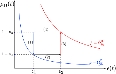
Figure 3: (Color online) Pictorial representation of the Quantum Otto cycle in the configuration space $\rho_{11}(t):=\langle 1|\hat{\rho}(t)|1\rangle$ vs. the energy gap $\epsilon(t)$ in the ITT limit. Steps 1) and 3) correspond to thermalizations where ${\cal S}$ is kept in contact with the cold bath $\rm C$ and hot bath $\rm H$, respectively; steps 2) and 4) instead represent sudden quenches of the Hamiltonian gap.

Unless considering infinitesimal transformations where $\epsilon_{2}\simeq\epsilon_{1}$, it is clear that at variance with the Carnot cycle, in the Otto cycle the working medium ${\cal S}$ is always in a out-of-equilibrium state. Accordingly in this case the S-D approximation technique Cavina et al. (2017a) cannot be applied.

As for the Carnot cycle, the system exchange heat with the baths only during the steps 1) and 3). In particular exploiting the fact that now during the thermalization the Hamiltonian is kept constant we have

$$\Delta Q_{\rm C} = \int_{{\cal I}_{\rm C}}dQ_{\rm C}(t)=\text{Tr}[\Delta\hat{\rho}_{\rm C}\;{\hat{H}_{1}}]\;,$$

$$\Delta Q_{\rm H} = \int_{{\cal I}_{\rm H}}dQ_{\rm H}(t)=\text{Tr}[\Delta\hat{\rho}_{\rm H}\;{\hat{H}_{2}}]\;,$$ (55)

where for $j={\rm H,C}$, $\Delta\hat{\rho}_{j}$ represent the increment experienced by the system density during the associated step. Equations (55) are valid for any Otto cycle, but we can specify them for our case $\hat{H}_{1,2}=\frac{\epsilon_{1,2}}{2}\hat{\sigma}^{z}$. If we also allow infinite time for the thermalization stages (ITT limit), the states at the end of the steps 1) and 4) are the thermal states $\hat{\Omega}^{({\rm C})}_{\epsilon_{1}}$ and $\hat{\Omega}^{({\rm H})}_{\epsilon_{2}}$, respectively, but in general they do not need to. In this case we have

$$\Delta\hat{\rho}_{\rm C}=-\Delta\hat{\rho}_{\rm H}=\hat{\Omega}^{({\rm C})}_{\epsilon_{1}}-\hat{\Omega}^{({\rm H})}_{\epsilon_{2}}\;,$$ (56)

which replaced into (55) yields the identities

$$\Delta Q^{(0)}_{\rm H} := \epsilon_{2}(p_{\rm C}-p_{\rm H})\;,$$ (57)

$$\Delta Q^{(0)}_{\rm C} := \epsilon_{1}(p_{\rm H}-p_{\rm C})=-\frac{\epsilon_{1}}{\epsilon_{2}}\Delta Q^{(0)}_{\rm H}\;,$$ (58)

where we use the upper index “$(0)$” to indicate that these are the heat exchanged in the IIT regime, and we used asymptotic ground state probabilities for the two isochores, defined as in Eq.(22)

$$p_{\rm C}=\frac{1}{e^{-\beta_{\rm C}\epsilon_{1}}+1}\ ,\quad\quad p_{\rm H}=\frac{1}{e^{-\beta_{\rm H}\epsilon_{2}}+1}\ .$$ (59)

If we further assume the constraint

$$\beta_{\rm C}\epsilon_{1}\geq\beta_{\rm H}{\epsilon_{2}}\;,$$ (60)

$\Delta Q^{(0)}_{\rm H}$ turns out to be positive while $\Delta Q^{(0)}_{\rm C}$ is negative. The absorbed and released heat contributions can hence be identified as

$$Q_{\rm ABS} = \Delta Q^{(0)}_{\rm H}\geq 0\;,$$ (61)

$$Q_{\rm REL} = \Delta Q^{(0)}_{\rm C}=-\frac{\epsilon_{1}}{\epsilon_{2}}Q_{\rm ABS}\;,$$ (62)

leading to an efficiency

$$\eta_{\rm o}=\frac{Q_{\rm ABS}+Q_{\rm REL}}{Q_{\rm ABS}}=1-\frac{\epsilon_{1}}{\epsilon_{2}}\;,$$ (63)

which thanks to (60) is smaller than the corresponding Carnot efficiency (32). Departing from the ITT regime, corrections can be computed analogously to what done for the Carnot cycle when considering non quasi-static cycles. Specifically we can write

$${\eta} = 1+\frac{Q_{\rm REL}}{Q_{\rm ABS}}\simeq 1+\frac{\Delta Q^{(0)}_{\rm C}}{\Delta Q^{(0)}_{\rm H}}\frac{1+\Delta Q^{(1)}_{\rm C}/\Delta Q^{(0)}_{\rm C}}{1+\Delta Q^{(1)}_{\rm H}/\Delta Q^{(0)}_{\rm H}}$$ (64)

$$= 1-\frac{\epsilon_{1}}{\epsilon_{2}}\frac{1+\alpha_{\rm C}}{1+\alpha_{\rm H}}=1-(1-\eta_{\text{o}})\frac{1+\alpha_{\rm C}}{1+\alpha_{\rm H}}\;,$$

where now the $\Delta Q^{(1)}_{j}$s refer to first order corrections associated with the finite thermalization times, while the $\alpha_{j}$s are the associated ratios  $\Delta Q^{(1)}_{j}/\Delta Q^{(0)}_{j}$ analogous to those introduced in Eq. (35) for the S-D corrections of the Carnot cycle. In a similar way the power of the cycle can be expressed as in Eq. (36) yielding

$$P = \frac{{Q_{\rm ABS}}+{Q_{\rm REL}}}{\tau_{\rm C}+\tau_{\rm H}}\simeq\frac{{\Delta Q^{(0)}_{\rm C}}+{\Delta Q^{(0)}_{\rm H}}+{\Delta Q^{(1)}_{\rm C}}+{\Delta Q^{(1)}_{\rm H}}}{\tau_{\rm C}+\tau_{\rm H}}$$ (65)

$$= {\Delta Q^{(0)}_{\rm H}}\frac{\eta_{\text{o}}+\alpha_{\rm H}-(\epsilon_{1}/\epsilon_{2})\alpha_{\rm C}}{\tau_{\rm C}+\tau_{\rm H}}\;,$$

where $\tau_{\rm C}$ and $\tau_{\rm H}$ are the finite temporal durations of the steps 1) and 3) respectively, which for $\alpha_{j}=0$ gives the quasi-static result

$$P^{(0)}:={\Delta Q^{(0)}_{\rm H}}\frac{\eta_{\text{o}}}{\tau_{\rm C}+\tau_{\rm H}}=\dfrac{(\epsilon_{2}-\epsilon_{1})(p_{\rm C}-p_{\rm H})}{\tau_{\rm C}+\tau_{\rm H}}\;.$$ (66)

III.2.1 Exact FTT Otto Cycle

An application of the perturbative analysis (65) in the case of a general engine evolving under the action of the dissipation model (94), is presented in Appendix C . Due to the simplicity of the scheme however, this approach can be replaced by the exact finite-time solution of the problem, which we are going to present in the following.

Departing from the ITT regime the two thermalizations (isochores) of the Otto cycle become inevitably partial. To account for this effect, we represent the ground state populations of the working medium ${\cal S}$ at time $t$ after the beginning of the isochore with the $j$-th bath,

$$\rho_{00}(t):=\langle 0|\hat{\rho}(t)|0\rangle=p_{j}+\Delta_{j}f_{j}(t)\;,$$ (67)

where $p_{j}$ is the equilibrium probability (59) one would get in the strict ITT regime, and where $\Delta_{j}$ quantifies how out of equilibrium is the system at the beginning of the isochore. In this expression $f_{j}(t)$ is a function of $t$ that depends on the explicit details of the dynamics and which, by construction must fulfil the conditions $f_{j}(0)=1$ and $\lim_{t\rightarrow\infty}f_{j}(t)=0$ to ensure proper thermalization in the ITT regime. The parameters $\Delta_{\rm H}$ and $\Delta_{\rm C}$ are not completely independent and can be connected via the temporal durations, $\tau_{\rm C}$ and $\tau_{\rm H}$, of the two isochore. Indeed by invoking continuity conditions for the density matrix of $\mathcal{S}$ between the two isothermal strokes, we obtain

$$p_{\rm C}+\Delta_{\rm C}f_{\rm C}(\tau_{\rm C})=p_{\rm H}+\Delta_{\rm H}\ ,$$

$$p_{\rm H}+\Delta_{\rm H}f_{\rm H}(\tau_{\rm H})=p_{\rm C}+\Delta_{\rm C}\ ,$$ (68)

which in particular imply

$$p_{\rm C}-p_{\rm H}=\Delta_{\rm H}\bigg{(}\frac{1-f_{\rm C}(\tau_{\rm C})f_{\rm H}(\tau_{\rm H})}{1-f_{\rm C}(\tau_{\rm C})}\bigg{)}\ .$$ (69)

From Eq. (55) it follows now that the relative heat exchanged during the isochore can now be expressed as

$$\Delta Q_{\rm H} =-\epsilon_{2}\Delta_{\rm H}\int_{0}^{\tau_{\rm H}}\dot{f}_{\rm H} =-\epsilon_{2}\Delta_{\rm H}(f_{\rm H}(\tau_{\rm H})-1)\ ,$$ (70)

$$\Delta Q_{\rm C} =-\epsilon_{1}\Delta_{\rm C}\int_{0}^{\tau_{\rm C}}\dot{f}_{\rm C} =-\epsilon_{1}\Delta_{\rm C}(f_{\rm C}(\tau_{\rm C})-1)\ ,$$ (71)

which yields a power equal to

$$P=\dfrac{(\epsilon_{2}-\epsilon_{1})(p_{\rm C}-p_{\rm H})}{\tau_{\rm C}+\tau_{\rm H}}\;\dfrac{(1-f_{\rm H}(\tau_{\rm H}))(1-f_{\rm C}(\tau_{\rm C}))}{1-f_{\rm C}(\tau_{\rm C})f_{\rm H}(\tau_{\rm H})}\;,$$ (72)

where in the second line we used (69) and the expression (66) for the power of the cycle under ITT conditions (notice that as expected when $f_{j}(\tau_{j})=0$ then $P$ reduces to the value $P^{(0)}$ of Eq. (66)). This is the exact expression for $P$ which depends on the explicit form of $f_{j}$. It is worth observing that the first numerator $(\epsilon_{2}-\epsilon_{1})(p_{\rm C}-p_{\rm H})$ of Eq. (72) depends only on the model temperatures and gaps, hence fixing the efficiency it is possible to maximize the remaining independently, choosing the optimal length of the strokes.

IV Quantum Thermal Machines in the Non-Markovian regime

As we have explicitly discussed in Sec. II.2 the Markovian character of the system dynamics guarantees that the 2nd Law of thermodynamics is satisfied in the open quantum systems setting, i.e. the unavoidable loss of free energy of systems interacting with large baths. With this in mind, it is easy to realise that modelling the coupling of an engine with a non-Markovian bath may result as a pumping of free energy from the environment. For this reason, any acclaimed boost of performance in such a setting can be considered trivial, or even meaningless if not justified physically (e.g. using non-equilibrium baths). Therefore we choose to model the dynamics of the reservoir coupling in an overall Markovian framework, picturing an environment which contains some degrees of freedom who share correlations and interact with the working medium, such as to make its local dynamics non-Markovian; in this way we avoid any unjustified external resource draining. In such a set up indeed, Refs. Wilming et al. (2016); Lekscha et al. (2018); Perarnau-Llobet et al. (2018) show how this mechanism can only have detrimental effects from the point of view of quasi-static Thermodynamics: that is, without external free energy injections, the 2nd Law assures the Carnot efficiency is the maximal one. Nothing instead, has been stated from the point of view of FTT: even if lowering the maximal efficiency, there is still question on the effects on power and EMP, which are, from the practical point of view, much more interesting than pure maximal efficiency. Here we try to fill this gap, finding indeed that non-Markovian dynamics may have positive effects.

IV.1 The model

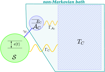
Figure 4: (Color online) Left: schematic of the non-Markovian model: ${\cal A}_{\rm H}$ and ${\cal A}_{\rm C}$ are local degrees of freedom of the hot and cold bath respectively. Right: specifics of the model, representation of the interaction between ${\cal S}$ and the non-Markovian cold bath.

In order to account for non-Markovian effects we consider a modification of the set-up of Sec. II.1, with the one schematically sketched in Fig. 4 where both the hot reservoir H and the cold reservoir C include a local and a remote component. The first, represented by the qubit ancillary subsystems ${\cal A}_{\rm H}$ and ${\cal A}_{\rm C}$ of the figure, corresponds to degrees of freedom characterized by local Hamiltonian terms

$$\hat{H}_{{\cal A}_{j}}:={E}_{j}\hat{\mathcal{\sigma}}^{z}_{{\cal A}_{j}}/2\;,$$ (73)

which are directly connected with $\mathcal{S}$ through dedicated coupling (energy exchanging) Hamiltonians which we assume to have the form

$$\hat{V}_{j}:=\gamma_{j}(\hat{\mathcal{\sigma}}^{+}\otimes\hat{\mathcal{\sigma}}_{{\cal A}_{j}}^{-}+\hat{\mathcal{\sigma}}^{-}\otimes\hat{\mathcal{\sigma}}_{{\cal A}_{j}}^{+})\;,$$ (74)

$\hat{\mathcal{\sigma}}_{{\cal A}_{j}}^{\pm}$ and $\hat{\mathcal{\sigma}}^{\pm}$ indicating the lowering/raising operators of ${\cal A}_{j}$ and ${\cal S}$ respectively. The remote components of the baths, instead, are associated with standard local GKSL dissipators ($\mathcal{D}_{t}^{(j)}$ for $\mathcal{S}$ , and $\mathcal{D}_{{\cal A}_{\rm C}}$ and $\mathcal{D}_{{\cal A}_{\rm H}}$ for ${\cal A}_{\rm H}$ and ${\cal A}_{\rm H}$, respectively) inducing local thermalization toward their associated Gibbs states, i.e. the usual canonical state $\hat{\Omega}^{(j)}_{\hat{H}_{t}}$ of (3) for ${\cal S}$, and for $j={\rm H,C}$,

$$\hat{\Omega}^{(j)}_{\hat{H}_{{\cal A}_{j}}}:=\frac{e^{-\beta_{j}{\hat{H}_{{\cal A}_{j}}}}}{\text{Tr}[e^{-\beta_{j}{\hat{H}_{{\cal A}_{j}}}}]}\;,$$ (75)

for ${\cal A}_{j}$. Once more, we shall consider cyclic operations where the gap of the local Hamiltonian of ${\cal S}$ is externally modulated as in Eq. (20), and the system, at each given time, is selectively coupled to one and only one of the two baths. Accordingly we describe the dynamics of joint density matrix $\hat{\mathbf{R}}(t)$ the compound formed by ${\cal S}$, ${\cal A}_{\rm C}$, and ${\cal A}_{\rm H}$, in terms of a standard Markovian evolution which has the same form of Eq. (1), the non-Markovian character of the local dynamics of $\mathcal{S}$ being obtained instead by tracing away the ancillas, i.e. $\hat{\rho}(t)=\mbox{Tr}_{\cal A}[\hat{\mathbf{R}}(t)]$ follows trajectories that no longer exhibit the divisibility condition that instead is granted to $\hat{\mathbf{R}}(t)$ – see Appendix F. Furthermore, in order to simplify the analysis we shall also enforce the approximation, that on the time intervals ${\cal I}_{\rm C}$ (resp. ${\cal I}_{\rm H}$) during which the working medium is coupled with the cold bath ${\rm C}$ (resp. ${\rm H}$), the other ancilla ${\cal A}_{\rm H}$ (resp. ${\cal A}_{\rm C}$), that is temporarily decoupled from ${\cal S}$, relaxes to thermal equilibrium with the remote counterpart of ${\rm H}$ (resp. ${\rm C}$), i.e.

$$\hat{\mathbf{R}}(t) \simeq \hat{\mathbf{R}}_{\rm C}(t)\otimes\hat{\Omega}^{(\rm H)}_{\hat{H}_{{\cal A}_{\rm H}}}\;,\qquad\forall t\in{\cal I}_{\rm C}\;,$$

$$\hat{\mathbf{R}}(t) \simeq \hat{\mathbf{R}}_{\rm H}(t)\otimes\hat{\Omega}^{(\rm C)}_{\hat{H}_{{\cal A}_{\rm C}}}\;,\qquad\forall t\in{\cal I}_{\rm H}\;,$$ (76)

with $\hat{\mathbf{R}}_{\rm C}(t)$ and $\hat{\mathbf{R}}_{\rm H}(t)$ that describe the reduced density matrix of of ${\cal S}{\cal A}_{\rm C}$ and ${\cal S}{\cal A}_{\rm H}$, respectively – the assumption being consistent with the first order S-D approximation, where ultimately one only needs to determine the quasi-static trajectories of the system rel . The evolution of $\hat{\mathbf{R}}_{j}(t)$ is finally expressed as

$$\dot{\hat{\mathbf{R}}}_{j}(t)=\mathcal{\bf L}_{t}^{(j)}[\hat{\mathbf{R}}_{j}(t)]:=-i[\hat{\bf H}_{t}^{(j)},\hat{\mathbf{R}}_{j}(t)]_{-}+\mathcal{\bf D}^{(j)}_{t}[\hat{\mathbf{R}}_{j}(t)]\ ,$$ (77)

with Hamiltonian

$$\hat{\bf H}_{t}^{(j)}:=\hat{H}_{t}+\hat{H}_{{\cal A}_{j}}+\hat{V}_{j}\;,$$ (78)

and dissipator

$$\mathcal{\bf D}^{(j)}_{t}:=\mathcal{D}_{t}^{(j)}\otimes{I}_{{\cal A}_{j}}+{I}\otimes\mathcal{D}_{{\cal A}_{j}}\;,$$ (79)

whose local contributions on ${\cal S}$ and on ${\cal A}_{j}$ will be assumed to have the simple form (94), i.e.

$$\mathcal{D}_{t}^{(j)}[\cdots] = \Gamma_{j}(\hat{\Omega}^{(j)}_{\hat{H}_{t}}-\cdots)\ ,$$ (80)

$$\mathcal{D}_{{\cal A}_{j}}[\cdots] = \Gamma_{{\cal A}_{j}}(\hat{\Omega}_{\hat{H}_{{\cal A}_{j}}}-\cdots)\ ,$$ (81)

where $\hat{\Omega}^{(j)}_{\hat{H}_{t}}$ and $\hat{\Omega}^{(j)}_{\hat{H}_{{\cal A}_{j}}}$ are the Gibbs states of (3) and (75) while $\Gamma_{j}$ and $\Gamma_{{\cal A}_{j}}$ are rates. As evident from the above expressions, we are assuming control on the energy gap of the working medium but not on the one of ${\cal A}_{j}$ which formally is just an element of the bath. We finally stress that $\gamma_{j}$ in Eq. (74) is the parameter defining the non-Markovianity of the model: this follows from the fact that the Markovian regime is recovered in the limit $\gamma_{j}\rightarrow 0$ (separable dynamics) and from the fact that, as shown in Appendix F, the non-Markovian measure by Breuer, Laine, Piilo Breuer et al. (2016) is monotonously increasing in $\gamma_{j}$. As we shall see in the next section a similar dependence can be observed on the optimized power output of a Carnot and Otto engine providing hence a clear indication of the fact that the non-Markovian character of the dynamics can be beneficial to these figures of merit.

IV.2 Non-Markovian Carnot cycle performance

In what follows we focus on the quasi-resonant case where the gap modulations of ${\cal S}$ on the interval ${\cal I}_{j}$ are such that the system is almost at resonance with ${\cal A}_{j}$, i.e.

$$\epsilon(t)\simeq E_{j}\;,\qquad\qquad\forall t\in{\cal I}_{j}\;$$ (82)

(note that the optimal Quasi-Otto trajectories found in Section III.1 are obtained in the limit of $\epsilon(t)$ being infinitesimally modulated). In this regime the stationary state of $\mathcal{\bf L}^{(j)}_{t}$ is approximatively equal to the tensor product of the individual thermal states associated with the two local dissipators, i.e.

$$\mathcal{\bf L}^{(j)}_{t}[\hat{\mathbf{R}}_{j}]=0\;\;\Leftrightarrow\;\;\hat{\mathbf{R}}_{j}\simeq\hat{\Omega}^{(j)}_{\hat{H}_{t}}\otimes\hat{\Omega}^{(j)}_{\hat{H}_{{\cal A}_{j}}}\;,$$ (83)

ensuring thermodynamic consistency of the model and being in agreement with Eq. (76). We hence identify the heat absorbed by ${\cal S}$ from the $j$-th bath as in Eq. (9) we obtain

$$dQ_{j}(t) = \text{Tr}\Big{[}\hat{H}_{t}d\hat{\rho}(t)\Big{]}=\text{Tr}\Big{[}\hat{H}_{t}d\hat{\mathbf{R}}_{j}(t)\Big{]}\;,$$ (84)

where in the first identity we used the fact that $\hat{\rho}(t)$ is the partial trace with respect to ${\cal A}_{j}$ of $\hat{\mathbf{R}}_{j}(t)$. We then expand this quantity as in Eq. (17) by invoking the S-D approximation $\hat{\mathbf{R}}_{j}(t)\simeq\hat{\mathbf{R}}^{(0)}_{j}(t)+\hat{\mathbf{R}}^{(1)}_{j}(t)+\cdots$, where $\hat{\mathbf{R}}^{(0)}_{j}(t)$ is the quasi-static solution which according to (83) is the state $\hat{\Omega}^{(j)}_{\hat{H}_{t}}\otimes\hat{\Omega}^{(j)}_{\hat{H}_{{\cal A}_{j}}}$, while $\hat{\mathbf{R}}^{(1)}_{j}(t)$ is the first order correction term which according to Eq. (16) we identify with the operator

$$\hat{\mathbf{R}}^{(1)}_{j}(t)=(\mathcal{\bf L}^{(j)}_{t}\mathcal{P})^{-1}[\dot{\hat{\mathbf{R}}}^{(0)}_{j}(t)]\,.$$ (85)

Due to the factorization of the fixed point (83) the zero-th term contribution $dQ^{(0)}_{j}(t)$ of $dQ_{j}(t)$ is still provided by the increment of the von Neumann entropy of the Gibbs states $\hat{\Omega}^{(j)}_{\hat{H}_{t}}$ as in Eq. (18). On the contrary $dQ^{(1)}_{j}(t)$ can still be cast in the form (38) where now ${\rho}^{(1)}_{00}(t)=\langle 0|\mbox{Tr}_{{\cal A}_{j}}[\hat{\mathbf{R}}^{(1)}_{j}(t)]|0\rangle$ that in the limit (82) can be expressed as in Eq. (39) with an S-D amplitude $A_{j}$ that can be found (see Appendix E.2) equal to

$$A_{j}=\dfrac{1/\Gamma_{j}}{(c_{j}+1)^{2}}\bigg{(}2+\dfrac{c_{j}(c_{j}-2)}{(c_{j}+2y_{j}^{2})}+\dfrac{c_{j}^{2}(c_{j}+1)^{2}-c_{j}^{3}}{(c_{j}+2y_{j}^{2})^{2}}\bigg{)}\ ,$$ (86)

where we introduce the quantities

$$c_{j}:=\Gamma_{{\cal A}_{j}}/\Gamma_{j}\;,\qquad y_{j}:=\gamma_{j}/\Gamma_{j}\;.$$ (87)

To evaluate the effect of non-Markovianity on the maximum power associated with a Carnot cycle we can then follow the same analysis we performed in Sec. III.1.1. In particular under symmetrization of the bath couplings and driving conditions (i.e. choosing $A_{\rm C}=A_{\rm H}=A$ and imposing $\epsilon(t)$ along the cold isotherm to be the time reversal of the one along the hot isotherm), we can directly use Eq. (53), which makes it clear that to get higher power performance we should target the low values of the $A_{j}$s.

First of all we notice that for $\gamma_{j}=0$ (i.e. $y=0$) correctly reduces to $A_{j}={1}/{\Gamma_{j}}$, which is the value (40) one would obtained in the Markovian limit in the presence of the dissipator (80). In the strong coupling limit $\gamma_{j}\gg\Gamma_{j}$ (i.e. $y_{j}\gg 1$), instead we get

$$A_{j}^{\rm(strong)}:=\lim_{y_{j}\rightarrow\infty}A_{j}=(2/\Gamma_{j})/(c_{j}+1)^{2}\;,$$ (88)

which gets smaller than the non-Markovian limit for values of $c_{j}$ above the critical threshold $\sqrt{2}-1\simeq 0.414$. Another important value is $c_{j}=2$ that determines the sign of the second addend in the parenthesis in the r.h.s. of Eq. (86) (the third addend being always positive). In fact we find that for $c_{j}<2$, $A_{j}$ attains its minimum value, smaller than the Markovian $1/\Gamma_{j}$, at

$$y_{j,opt}^{2}=\frac{c_{j}^{2}(2c_{j}+3)}{2(2-c_{j})}\ ,$$ (89)

otherwise the optimal value is infinite, in the sense of $A_{j}$ monotonously decreasing with $y_{j}$. These results on the dependence of $A_{j}$ on the model parameters are summed up in the Fig. 5, where we plot $A_{j}^{-1}$ in adimensional units, which thanks to Eq.s (50) and (53) corresponds to the maximum power attainable by the Carnot cycle, normalized to its Markovian value. In each case we see how the presence of the coupling $\gamma_{j}$, i.e. of non-Markovian effects leads to the an improvement of the maximum power $P_{\max}$ of the Carnot cycle.

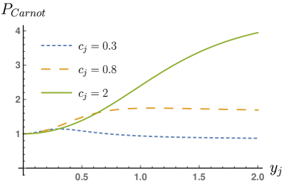
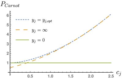
Figure 5: (Color online) Upper panel: Maximum power of the Carnot cycle normalized to its Markovian value, in terms of the parameter $y_{j}$ that accounts for the non-Markovian effects in the model. The plot corresponds to $A_{j}^{-1}$ of Eq. (86) in units of $\Gamma_{j}$. For $0\leq c_{j}\leq\sqrt{2}-1$: there exists an optimal $y_{j}$ but for $y_{j}\rightarrow\infty$, $A_{j}^{-1}$ is inferior to the initial value $\Gamma_{j}$. For $\sqrt{2}-1\leq c_{j}\leq 2$: there exists an optimal $y$ and for $y_{j}\rightarrow\infty$, $A_{j}^{-1}$ remains bigger than the Markov case. For $2\leq c_{j}$: there is no finite optimal value for $y_{j}$, but $A_{j}^{-1}$ continues growing to its asymptotic value. Lower panel: comparison of $A_{j}^{-1}$ (in units of $\Gamma_{j}$) as a function of $c_{j}$ having fixed $y_{j}$ equal to the optimal choice (89) (blue) with the Markovian case $\gamma_{j}=0$ (green) and strong-coupling case $\gamma_{j}=\infty$ (yellow).

IV.3 Non-Markovian Otto cycle performance

To study the performance of an Otto cycle for the non-Markovian model introduced, we can apply the exact power result (72), which in turn is characterized by the function $f_{j}$ describing the relaxation of the ground state during the two isochores ($j=\rm H,C$) (cf. Eq. (67)). In this case we restrict ourself to case $\Gamma_{{\cal{A}}_{j}}=\Gamma_{j}$ in resonance conditions between the system $\mathcal{S}$ and the ancillas, i.e. $\epsilon_{1}=E_{\rm C}$ and $\epsilon_{2}=E_{\rm H}$. As shown in Appendix E.1, under these conditions (82), the model allows for simple analytical solution of the form

$$f_{j}(t)=\frac{e^{-t}}{2}+e^{(-\frac{3}{2}+\frac{\kappa_{j}}{2})t}\bigg{(}\frac{1+\kappa_{j}}{4\kappa_{j}}\bigg{)}-e^{(-\frac{3}{2}-\frac{\kappa_{j}}{2})t}\bigg{(}\frac{1-\kappa_{j}}{4\kappa_{j}}\bigg{)}\ ,$$ (90)

where to simplify the notation the time has been expressed in units of $\Gamma_{j}^{-1}$ and where $\kappa_{j}:=\sqrt{1-16(\gamma_{j}/\Gamma_{j})^{2}}$. As for the previous example we enforce symmetric conditions in which the couplings to the thermal baths have the same Lindbladian form and strength, i.e. $\Gamma_{\rm H}=\Gamma_{\rm C}$ and $\gamma_{\rm H}=\gamma_{\rm C}$, implying $f_{\rm C}(t)=f_{\rm H}(t)=f(t,\kappa)$. Under this assumption it is not difficult to prove (see Appendix G) that the maximum value of the power obtainable from (72) is found on the bisector $\tau_{\rm C}=\tau_{\rm H}=\tau$. Specifically with this choice we get

$$P=\frac{(E_{\rm H}-E_{\rm C})(p_{\rm C}-p_{\rm H})}{2\tau}\frac{1-f(\tau,\kappa)}{1+f(\tau,\kappa)}\;,$$ (91)

which for each value of $\kappa(y)$ has a maximum for a finite value of the duration $\bar{\tau}(y)$. In Fig. 6 we plot the obtained maximum as a function of $y=\gamma/\Gamma$, normalized to the $\gamma=0$ case, for which Eq. (91) is easily seen to have a maximum equal to $\frac{\Gamma}{4}(E_{\rm H}-E_{\rm C})(p_{\rm C}-p_{\rm H})$. As in the case of the Carnot cycle we see once more that increasing the strength of the non-Markovian coupling parameter $\gamma$ the power of the Otto engine dramatically increases.

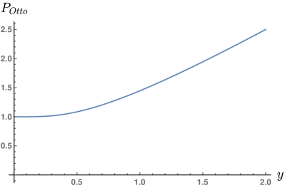
Figure 6: Maximum power for the non-Markovian Otto cycle (91), as a function of $\gamma/\Gamma$, in units of $\frac{\Gamma}{4}(E_{\rm H}-E_{\rm C})(p_{\rm C}-p_{\rm H})$ (Markovian value).

IV.4 Free-energy analysis

Ruling out the possibility of using non-Markovian effects to improve the efficiency in the model  Wilming et al. (2016); Lekscha et al. (2018); Perarnau-Llobet et al. (2018), the power boost we reported above for the Carnot and Otto cycle can only be seen as a consequence of the latter in the reduction of thermalization timescales. We show here an argument to explain why it happens and how it is related to the non-Markovian building of correlations between the engine $\mathcal{S}$ and the $j$-th bath.

When attaching $\mathcal{S}$ to the $j$-th bath, the former is out of equilibrium, while according to Eq. (76) $\mathcal{A}_{j}$ is already thermalized: we can hence describe their initial state as $\hat{\rho}(0)\otimes\hat{\Omega}^{(j)}_{\hat{H}_{\mathcal{A}_{j}}}$. A possible way to quantify the rapidity of $\mathcal{S}$ thermalizing is to compute the relative entropy $S(\hat{\rho}(t)\parallel\hat{\Omega}^{(j)}_{\hat{H}_{t}})$ and see how fast it diminishes. We recall that according to (12) this quantity also measures the excess of free energy present in the system from the corresponding Gibbs state at temperature $T_{j}$. Indicating hence with $\hat{\mathbf{R}}_{j}(t)$ the joint state of ${\cal S}$ and ${\cal A}_{j}$ at time $t$ we notice that

$$S(\hat{\mathbf{R}}_{j}(t)\parallel\hat{\Omega}^{(j)}_{\hat{H}_{t}}\otimes\hat{\Omega}^{(j)}_{{\cal A}_{j}}) = S(\hat{\rho}(t)\parallel\hat{\Omega}^{(j)}_{\hat{H}_{t}})+S(\hat{\rho}_{{\cal A}_{j}}(t)\parallel\hat{\Omega}^{(j)}_{{\cal A}_{j}})$$ (92)

$$+ I(\mathcal{S}:\mathcal{A}_{j})/\beta_{j}\ ,$$

where $I(\mathcal{S}:\mathcal{A}_{j})\geq 0$ is the mutual information Holevo (2012) between the two systems at time $t$ (in the above derivation we explicitly use the fact that the mean value of the interaction term stays null due to the quasi-resonant conditions assumptions). Hence the variation of the free energy of $\mathcal{S}$ can be expressed as

$$\Delta S(\hat{\rho}(t)\parallel\hat{\Omega}^{(j)}_{\hat{H}_{t}}) = \Delta S(\hat{\mathbf{R}}_{j}(t)\parallel\hat{\Omega}^{(j)}_{\hat{H}_{t}}\otimes\hat{\Omega}^{(j)}_{{\cal A}_{j}})$$

$$- \Delta S(\hat{\rho}_{{\cal A}_{j}}(t)\parallel\hat{\Omega}^{(j)}_{{\cal A}_{j}})-\Delta I(\mathcal{S}:\mathcal{A}_{j})/\beta_{j}\ .$$

Now we observe that the last two terms provide a negative contributions to $\Delta S(\hat{\rho}(t)\parallel\hat{\Omega}^{(j)}_{\hat{H}_{t}})$. Indeed being the relative entropy and mutual information positive definite, and being the initial state of ${\cal S}$ and ${\cal A}_{j}$ factorized by hypothesis, they are initially null, meaning that they can only increase with time, thus bringing negative contribution to the r.h.s. of (IV.4), that is faster thermalization of ${\cal S}$. For a comparison, in case $\mathcal{S}$ and $\mathcal{A}_{j}$ do not interact (that is $\gamma=0$ in our model) mutual information would remain zero and $\hat{\rho}_{{\cal A}_{j}}$ would stay thermal making these two terms exactly null. In support of the above analysis we report in Fig. 7 an example of an evolution of the above quantities. It is possible to see how the free energy of $\mathcal{S}$ decreases faster than the total free energy, due to ”suction of free energy” by $\mathcal{A}_{j}$ and the correlations $I(\mathcal{S}:\mathcal{A}_{j})$ building.

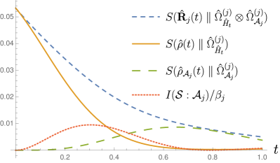
Figure 7: (Color online) The total free energy (normalized to 0) $F_{{\cal S}{\cal A}_{j}}=S(\hat{\mathbf{R}}_{j}(t)\parallel\hat{\Omega}^{(j)}_{\hat{H}_{t}}\otimes\hat{\Omega}^{(j)}_{{\cal A}_{j}})$ (upper line, dashed blue), with its decomposition in the local free energies and the correlation term $S(\hat{\rho}(t)\parallel\hat{\Omega}^{(j)}_{\hat{H}_{t}})+S(\hat{\rho}_{{\cal A}_{j}}(t)\parallel\hat{\Omega}^{(j)}_{{\cal A}_{j}})+I(\mathcal{S}:\mathcal{A}_{j})/\beta_{j}$, decreasing in time (in units of $\Gamma^{-1}$). The free energy of $\mathcal{S}$ (yellow) decays faster due to the free energy of ${\cal A}_{j}$ (green, dashed) and the system-bath correlations (red, dotted) growing. Energies are in units of $\epsilon=E_{j}$. $T_{j}=2.5$. The initial state is given by $\hat{\rho}(0)\otimes\hat{\Omega}^{(j)}_{\hat{H}_{\mathcal{A}_{j}}}$ with ground state populations ${\rho}_{00}(0)=0.7$, and $[\hat{\Omega}^{(j)}_{\hat{H}_{\mathcal{A}_{j}}}]_{00}=0.6$ respectively, and the non-Markovian parameter $y_{j}=2$.

V Conclusions

The purpose of the work is to assess the effects of non-Markovian dynamics on quantum thermal machines. We considered a simple class of models which allows shared correlation between the system and some degrees of belonging to the baths, preserving the global evolution as Markovian. This avoids resource pumping from the baths, and cannot induce advantages from the quasi-static point of view. Exploiting the S-D technique we studied the thermodynamic performance for a (finite-time) Carnot cycle: results indicate that the maximum power can indeed be boosted by the presence of this non-Markovian mechanism. Exact results obtained by studying Otto cycles confirm this trend. Noting that in general the S-D amplitude $A$ is related to the relaxation time of the system, we are naturally led to interpret this positive effect as an acceleration of the thermalization timescale of ${\cal S}$, in presence of its possible interaction with the local components of the baths (cf. Fig.4). Again this is intuitively reasonable, having $\mathcal{S}$ a new channel of thermalization which passes through $\mathcal{A}_{j}$, and we showed explicitly in Sec. IV.4 how this effect is related to the non-Markovian feature of the baths building correlations with the working medium.

Preliminary to the results, we also showed how to optimize the control for a 2-level engine performing a Carnot cycle (in the low-dissipation regime) or an Otto cycle (exactly).

A possible extension of the research would be to generalize these results for systems beyond qubits, with variable number of levels or in the geometrical picture introduced in Scandi and Perarnau-Llobet (2018); Abiuso and Perarnau .

Appendix A The dissipators

Here we review few examples of dissipators $\mathcal{D}_{t}^{(j)}$ that obey the constraints (2) and (4).

The first, and simplest of such models, is provided by the super-operator Cavina et al. (2017b)

$$\mathcal{D}_{t}^{(j)}[\cdots]=\Gamma_{j}(\hat{\Omega}^{(j)}_{\hat{H}_{t}}-\cdots)\;,\\$$ (94)

with $\Gamma_{j}>0$ constant, which do not need any specification of the system Hamiltonian.

Assuming instead the Hamiltonian of ${\cal S}$ to be $\hat{H}_{t}={\epsilon}(t)\hat{\mathcal{\sigma}}^{z}/2$ (see Eq. (20)), another example is provided by the dissipator

$$\mathcal{D}_{t}^{(j)}[\cdots]:=\sum_{\ell=\pm}\Gamma^{(j)}_{\ell}(\epsilon(t))(\hat{\sigma}_{\ell}\cdots\hat{\sigma}_{\ell}^{\dagger}-\frac{1}{2}[\hat{\sigma}_{\ell}^{\dagger}\hat{\sigma}_{\ell},\cdots]_{+})\;,$$ (95)

where $\hat{\sigma}_{+}$ and $\hat{\sigma}_{-}(=\hat{\sigma}_{+}^{\dagger})$ are, respectively, the raising and lowering operators of ${\cal S}$, $[\cdots,\cdots]_{+}$ is the anti-commutator, which exhibit the functional dependence (2) upon $\hat{H}_{t}$ through the rates $\Gamma^{(j)}_{\pm}(\epsilon)$ fulfilling the detailed balance equation condition

$${\Gamma^{(j)}_{+}(\epsilon)}/{\Gamma^{(j)}_{-}(\epsilon)}=e^{-\beta_{j}\epsilon}\;,$$ (96)

which ensures (4). In particular taking

$$\Gamma^{(j)}_{-}(\epsilon):=(1-N_{\bf F}(\beta_{j}\epsilon))\;\Gamma\;,\quad\Gamma^{(j)}_{+}(\epsilon):=N_{\bf F}(\beta_{j}\epsilon)\;\Gamma\;,$$

with $\Gamma\geq 0$ and

$$N_{\bf F}(x)=\frac{1}{e^{x}+1}\;,$$ (97)

equation (95) can be used to describe the interaction of ${\cal S}$ with a Fermionic bath. Instead taking

$$\Gamma^{(j)}_{-}(\epsilon):=(1+N_{\bf B}(\beta_{j}\epsilon))\;\Gamma\;,\quad\Gamma^{(j)}_{+}(\epsilon):=N_{\bf B}(\beta_{j}\epsilon)\;\Gamma\;,$$

with $\Gamma\geq 0$ and

$$N_{\bf B}(x)=\frac{1}{e^{x}-1}\;,$$ (98)

it describes the interaction of ${\cal S}$ with a Bosonic bath.

Appendix B S-D approximation implies low dissipation

A virtue of the S-D approximation is that it provides a formal justification of the low-dissipation (L-D) assumption Esposito et al. (2010) which is typically introduced in FTT analysis as a phenomenological working hypothesis. To see this let us start observing that in the S-D theory, at the lowest order of the pertubative expansion (15) the von Neumann entropy of the density matrix $\hat{\rho}(t)$ can be expressed as

$$S(t):=\mbox{Tr}[\hat{\rho}(t)\ln\hat{\rho}(t)]\simeq\mbox{Tr}[(\hat{\rho}^{(0)}(t)+\hat{\rho}^{(1)}(t))\ln(\hat{\rho}^{(0)}(t)+\hat{\rho}^{(1)}(t))]\simeq S^{(0)}(t)+\beta_{j}\text{Tr}[\hat{\rho}^{(1)}(t)\hat{H}_{t}]\;,$$ (99)

where in the last step we used the fact that the term $\hat{\rho}^{(1)}(t)$ is traceless, i.e. $\text{Tr}[\hat{\rho}^{(1)}(t)]=0$, and the fact that $\hat{\rho}^{(0)}(t)$ is the instantaneous Gibbs state (3), i.e. $\hat{\rho}^{(0)}(t)=\hat{\Omega}^{(j)}_{\hat{H}_{t}}$. A close inspection reveals that the second contribution of $S(t)$ corresponds to the first order correction to the internal energy of the system defined in Eq. (7), i.e. $E_{1}(t):=\text{Tr}[\hat{\rho}^{(1)}(t)\hat{H}_{t}]$, allowing us to cast (99) as

$$S(t)\simeq S^{(0)}(t)+\beta_{j}E^{(1)}(t)\ .$$ (100)

The temporal increment of this quantity can hence be computed as

$$dS(t)\simeq dS^{(0)}(t)+\beta_{j}dE^{(1)}(t)=\beta_{j}dQ^{(0)}(t)+\beta_{j}dQ^{(1)}(t)+\beta_{j}dW^{(1)}(t)\;,$$ (101)

where we used Eq. (18) and wrote $dE^{(1)}(t)$ in terms of a work and heat contribution, i.e. $dE^{(1)}(t)=dQ^{(1)}(t)+dW^{(1)}(t)$ (first thermodynamics principle) with $dQ^{(1)}(t)$ as in Eq. (19) and

$$dW^{(1)}(t):=\text{Tr}[\hat{\rho}^{(1)}(t)d\hat{H}_{t}]\;.$$ (102)

Grouping together all the heat contributions we can hence finally write

$$dS(t)\simeq\beta_{j}dQ(t)+\beta_{j}dW^{(1)}(t)\,\Longrightarrow dS^{(irr)}_{j}(t)\simeq\beta_{j}dW^{(1)}(t)\;,$$ (103)

where $dS^{(irr)}_{j}(t):=dS(t)-\beta_{j}dQ(t)$ is the irreversible entropy production increment which quantifies the differences between information transfer rates and the heat transfer rate in the system. When integrated over a finite time interval $\tau_{j}$, Eq. (103) provides an estimation of the associated finite irreversible entropy production $\Delta S^{(irr)}_{j}$. In FTT under L-D assumption this term is postulated to be expressed as inversely proportional to $\tau_{j}$ via a constant term $\Sigma_{j}$ which only depends on the coupling constants to the bath, and the cycle endpoints, i.e. Esposito et al. (2010); Ma et al. (2018)

$$\Delta S^{(irr)}_{j}\Big{\rvert}_{\rm L-D}=\Sigma_{j}/\tau_{j}\;.$$ (104)

Now a $1/\tau_{j}$ scaling as in Eq. (104) is exactly what one naturally get by computing $\Delta S^{(irr)}_{j}$ via direct integration of (103) due to the fact that in the S-D expansion the $\hat{\rho}^{(1)}(t)$ term has an explicit linear dependence upon $1/\tau_{j}$, whilst $\hat{\rho}^{(0)}(t)$ and the associated instantaneous Hamiltonian $\hat{H}_{t}$ are independent from such parameter Cavina et al. (2017a, 2018). According to this observation, on one side we can hence say that S-D provide a natural framework for discussing L-D assumption. On the other side instead we can conclude that the general results derived under FTT assumption Esposito et al. (2010); Ma et al. (2018) must apply in the characterization of system driven under S-D approximation, at least at the first order of the perturbative analysis. In particular it is not difficult to see that the condition $\alpha_{\rm C}=\alpha_{\rm H}$ we require in Sec. III.1 corresponds to set $\Sigma_{\rm C}=\Sigma_{\rm H}$, which in turn implies that the Curzon-Ahlborn efficiency is the EMP in this regime Esposito et al. (2010). Getting rid of this symmetry simply means to explore the different ratios $\Sigma_{\rm H}/\Sigma_{\rm C}$ and the relative results Esposito et al. (2010); Ma et al. (2018) are valid.

Appendix C Otto cycle beyond the ITT limit

To evaluate the correction terms appearing in Eqs. (64) and (65) for a generic engine we assume the dissipation model of Eq. (94). Let then indicate with $\hat{\rho}^{(in)}_{j,k}$ and $\hat{\rho}^{(out)}_{j,k}$ the states of ${\cal S}$ at the beginning and at the end of the time intervals ${\cal I}_{j}$ of the $k$-th Otto cycle. Due to the presence of the quenches at the steps 2) and 4), they must be related as follows

$$\hat{\rho}^{(in)}_{{\rm H},k}=\hat{\rho}^{(out)}_{{\rm C},k}\;,\qquad\hat{\rho}^{(in)}_{{\rm C},k}=\hat{\rho}^{(out)}_{{\rm H},k-1}\;,$$ (105)

meaning that input state of the $k$-th interval ${\cal I}_{\rm H}$ coincides with the output state of the $k$-th interval ${\cal I}_{\rm C}$, while the input of the $k$-th interval ${\cal I}_{\rm C}$ with the output of the $k$-th interval ${\cal I}_{\rm H}$. By direct integration of the ME (1) we get

$$\hat{\rho}^{(out)}_{{\rm C},k}=\hat{\Omega}^{({\rm C})}_{\epsilon_{1}}+e^{-\Gamma_{\rm C}\tau_{\rm C}}(\hat{\rho}^{(in)}_{{\rm C},k}-\hat{\Omega}^{({\rm C})}_{\epsilon_{1}})\;,\qquad\hat{\rho}^{(out)}_{{\rm H},k}=\hat{\Omega}^{({\rm H})}_{\epsilon_{2}}+e^{-\Gamma_{\rm H}\tau_{\rm H}}(\hat{\rho}^{(in)}_{{\rm H},k}-\hat{\Omega}^{({\rm H})}_{\epsilon_{2}})\;,$$ (106)

which, with the help of (105) can be equivalently cast in the following recursive expressions

$$\hat{\rho}^{(out)}_{{\rm C},k}=\hat{\Omega}^{({\rm C})}_{\epsilon_{1}} + e^{-\Gamma_{\rm C}\tau_{\rm C}}(\hat{\Omega}^{({\rm H})}_{\epsilon_{2}}-\hat{\Omega}^{({\rm C})}_{\epsilon_{1}})+e^{-(\Gamma_{\rm C}\tau_{\rm C}+\Gamma_{\rm H}\tau_{\rm H})}(\hat{\rho}^{(out)}_{{\rm C},k-1}-\hat{\Omega}^{({\rm C})}_{\epsilon_{1}})\;,$$ (107)

$$\hat{\rho}^{(out)}_{{\rm H},k}=\hat{\Omega}^{({\rm H})}_{\epsilon_{2}} - e^{-\Gamma_{\rm H}\tau_{\rm H}}(\hat{\Omega}^{({\rm H})}_{\epsilon_{2}}-\hat{\Omega}^{({\rm C})}_{\epsilon_{1}})+e^{-(\Gamma_{\rm C}\tau_{\rm C}+\Gamma_{\rm H}\tau_{\rm H})}(\hat{\rho}^{(out)}_{{\rm H},k-1}-\hat{\Omega}^{({\rm H})}_{\epsilon_{2}})\;.$$ (108)

Now in the ITT limit $\tau_{j}\rightarrow\infty$ these yields $\hat{\rho}^{(out)}_{{\rm C},k}=\hat{\Omega}^{({\rm C})}_{\epsilon_{1}}$ and $\hat{\rho}^{(out)}_{{\rm H},k}=\hat{\Omega}^{({\rm H})}_{\epsilon_{2}}$ for all $k$, leading to (111) via Eq. (105). For finite $\tau_{j}$ instead, keeping only the most relevant order, we obtain

$$\hat{\rho}^{(out)}_{{\rm C},k} \simeq \hat{\Omega}^{({\rm C})}_{\epsilon_{1}}+e^{-\Gamma_{\rm C}\tau_{\rm C}}(\hat{\Omega}^{({\rm H})}_{\epsilon_{2}}-\hat{\Omega}^{({\rm C})}_{\epsilon_{1}})\;,$$ (109)

$$\hat{\rho}^{(out)}_{{\rm H},k} \simeq \hat{\Omega}^{({\rm H})}_{\epsilon_{2}}-e^{-\Gamma_{\rm H}\tau_{\rm H}}(\hat{\Omega}^{({\rm H})}_{\epsilon_{2}}-\hat{\Omega}^{({\rm C})}_{\epsilon_{1}})\;,$$ (110)

for all $k$, which, exploiting once more (105), gives

$$\Delta\hat{\rho}_{\rm C}=-\Delta\hat{\rho}_{\rm H}\simeq(1-e^{-\Gamma_{\rm C}\tau_{\rm C}}-e^{-\Gamma_{\rm H}\tau_{\rm H}})(\hat{\Omega}^{({\rm C})}_{\epsilon_{1}}-\hat{\Omega}^{({\rm H})}_{\epsilon_{2}})\;.$$ (111)

Inserting this into Eq. (55) we can express the first order corrections $\Delta Q^{(1)}_{j}$s as

$$\Delta Q^{(1)}_{j}=-(e^{-\Gamma_{\rm C}\tau_{\rm C}}+e^{-\Gamma_{\rm H}\tau_{\rm H}})\Delta Q^{(0)}_{j}\;,$$ (112)

hence obtaining

$$\alpha_{j}=-(e^{-\Gamma_{\rm C}\tau_{\rm C}}+e^{-\Gamma_{\rm H}\tau_{\rm H}})\;,$$ (113)

for $j={\rm H,C}$. From Eq. (64) then follows that the efficiency remains un-effected by the ITT corrections, i.e. $\eta=\eta_{\text{o}}$, while according to Eq. (66) the power becomes

$$P\simeq{\Delta Q^{(0)}_{\rm H}}\frac{\eta_{\text{o}}-\eta_{\text{c}}(e^{-\Gamma_{\rm C}\tau_{\rm C}}+e^{-\Gamma_{\rm H}\tau_{\rm H}})}{\tau_{\rm C}+\tau_{\rm H}}\;.$$ (114)

Appendix D Optimal protocol shape for the Quantum Carnot cycle

In this section we solve the minimization of the functional ${\cal F}[q(x)]$ of (51) (hereby ${\cal F}[q]$ for short) under the constraints

$$\{q(0)=q_{in}\;,\dot{q}(0)=0\;,q(1)=q_{fin}\;,\dot{q}(1)=0\},$$ (115)

which, according to Eq. (50) allow us to optimize the power production on the Quantum Carnot cycle. First of all we notice that it can be equivalently expressed as

$${\cal F}[q]=-\int_{0}^{1}\text{d}x\ \ddot{q}\ln\big{(}\frac{q}{1-q}\big{)}\;,$$ (116)

where the modulus has been replaced by a minus sign, due to the fact that integrand is guaranteed to be non-positive for all the allowed choices of the function $q(x)$ (same argument we used in Eq. (41) to establish the non positivity of $\Delta Q_{j}^{(1)}$).

For this purpose we consider the variation of the functional (51) under a small variation of the control $q\rightarrow q+\delta q$,

$$\delta{\cal F}[q]={\cal F}[q+\delta q]-{\cal F}[q]=-\int\delta\ddot{q}\ln\big{(}\frac{q}{1-q}\big{)}+\int\ddot{q}\ \delta\!\ln\big{(}\frac{q}{1-q}\big{)}=-\int\delta q\bigg{[}\frac{2\ddot{q}}{q(1-q)}+\dot{q}^{2}\frac{2q-1}{q^{2}(1-q)^{2}}\bigg{]}\;,$$ (117)

where the last identity was obtained by integration by parts using the constraints 115. Imposing the latter to nullify under arbitrary variation we can then obtain the differential equation

$$2\ddot{q}+\dot{q}^{2}\frac{2q-1}{q(1-q)}=0\quad\Longrightarrow\quad 2\ln\dot{q}-\ln(q(1-q))=constant\ ,$$ (118)

which can be solved using separation of variables and the substitution $q^{\prime}=q-\frac{1}{2}$, leading to optimal solutions of the form

$$\bar{q}(x)=\cos^{2}\bigg{(}\frac{\omega(x+\varphi)}{2}\bigg{)}=\frac{1+\cos(\omega(x+\varphi))}{2}.$$ (119)

This class of solutions is parametrised by the two values $\{\omega,\varphi\}$ and is in general incompatible with the constraints 115 given at the extrema: this is a typical issue one meets in variational problems performed on given sets of functions that are not topologically closed; that is, it is possible to construct a sequence of functions $q_{k}(x)$ which decrease the functional toward an infimum which, however, is reached only for a function $\lim_{k\rightarrow\infty}q_{k}=\bar{q}$ that is outside the initial function space. We can build the sequence $q_{k}$ by simply stringing smoothly $\bar{q}(0)$ to $\bar{q}(\varepsilon)$ and $\bar{q}(1-\varepsilon)$ to $\bar{q}(1)$ for small $\varepsilon=\frac{1}{k}$,

$$q_{k}(x)=\begin{cases}s_{k}&0\leq x\leq\frac{1}{k}\\ \bar{q}(t)&\frac{1}{k}\leq x\leq 1-\frac{1}{k}\\ s_{k}&1-\frac{1}{k}\leq x\leq 1\end{cases}$$ (120)

with sufficiently smooth functions $s_{k}$ such that $s_{k}(0)=\bar{q}(0),\ s_{k}(\frac{1}{k})=\bar{q}(\frac{1}{k}),\ \dot{s}_{k}(0)=0,\ \dot{s}_{k}(\frac{1}{k})=\dot{\bar{q}}(\frac{1}{k})$ and similarly for $x=1-\frac{1}{k},1$. The correction to the optimal functional $\delta_{k}{\cal F}={\cal F}[{q_{k}}]-{\cal F}[{\bar{q}}]$ will then be given from the contribution near the border $[0,\frac{1}{k}]$

$$\int_{0}^{\frac{1}{k}}dx\Big{(}\ddot{s}_{k}\ln\big{(}\frac{s_{k}}{1-s_{k}}\big{)}-\ddot{\bar{q}}\ln\big{(}\frac{\bar{q}}{1-\bar{q}}\big{)}\Big{)}\sim\Big{(}\big{(}\dot{s}_{k}(\frac{1}{k})-\dot{s}_{k}(0)\big{)}\ln\big{(}\frac{s_{k}(0)}{1-s_{k}(0)}\big{)}-\big{(}\dot{\bar{q}}(\frac{1}{k})-\dot{\bar{q}}(0)\big{)}\ln\big{(}\frac{\bar{q}(0)}{1-\bar{q}(0)}\big{)}\Big{)}$$ (121)

and the analogous term for $[1-\frac{1}{k},1]$. Using that $\dot{s}_{k}(\frac{1}{k})-\dot{s}_{k}(0)=\dot{\bar{q}}(\frac{1}{k})$ we can take the limit to obtain, adding the $[1-\frac{1}{k},1]$ contribution,

$$\lim_{k\rightarrow\infty}\delta_{k}{\cal F}:=\bar{\delta}{\cal F}=\dot{\bar{q}}(0)\ln\bigg{(}\frac{\bar{q}(0)}{1-\bar{q}(0)}\bigg{)}-\dot{\bar{q}}(1)\ln\bigg{(}\frac{\bar{q}(1)}{1-\bar{q}(1)}\bigg{)}\$$ (122)

and thus the optimal value

$$\lim_{k\rightarrow\infty}{\cal F}[q_{k}]:={\cal F}_{min}={\cal F}[{\bar{q}}]+\bar{\delta}{\cal F}\ .$$ (123)

It is however important to stress that the sequence $q_{k}$ will eventually break the S-D approximation, having a high second derivative near 0 and 1. Hence one should ”stop” to a $k$ which is not too big to achieve these approximate results. Numerical plots support the achievability of the limit.

Quasi-Otto limit.

When allowing the control to vary the initial and final point $\{q(0),q(1)\}$, numerical plots show that the choice that maximizes the value of the power (50), which is equal to

$$\dfrac{(\sqrt{T_{H}}-\sqrt{T_{C}})^{2}}{4A}\dfrac{\Big{(}\int\dot{q}\ln\big{(}\frac{q}{1-q}\big{)}\Big{)}^{2}}{-\int\ddot{q}\ln\big{(}\frac{q}{1-q}\big{)}}\;,$$ (124)

is obtained in the limit of them being the same $q(1)-q(0)=\varepsilon\rightarrow 0$. In this limit $\bar{q}(x)$ (119) is essentially a line with $\dot{\bar{q}}\sim\frac{\bar{q}(1)-\bar{q}(0)}{1}-0=\varepsilon\;,$ hence the numerator of (124) is

$$\Big{(}\int\dot{\bar{q}}\ln(\bar{q}/(1-\bar{q}))\text{d}t\Big{)}^{2}\sim\ln\big{(}\frac{\bar{q}}{1-\bar{q}}\big{)}^{2}\varepsilon^{2}\ .$$ (125)

For the denominator ${\cal F}_{min}$ the contribution ${\cal F}[{\bar{q}}]$ nullifies while $\bar{\delta}{\cal F}$ can be estimated from (122) as

$$\dot{\bar{q}}\Big{(}\ln\big{(}\frac{\bar{q}(0)}{1-\bar{q}(0)}\big{)}-\ln\big{(}\frac{\bar{q}(1)}{1-\bar{q}(1)}\big{)}\Big{)}\sim\frac{\varepsilon^{2}}{\bar{q}(1-\bar{q})}\ ,$$ (126)

where we use $\dot{q}=\varepsilon$ and the derivative of $\ln(q/(1-q))$, which is $1/(q(1-q))$. We can then write (124) in this limit

$$P_{Quasi-Otto}=\dfrac{(\sqrt{T_{H}}-\sqrt{T_{C}})^{2}}{4A}[\ln\big{(}\dfrac{\bar{q}}{1-\bar{q}}\big{)}]^{2}\bar{q}(1-\bar{q})\ .$$ (127)

It is possible plot this function to find the optimal value of $\bar{q}$ around which to perform the optimal control, as in Figure 8, where is evident that $q_{optimal}\sim 0.92$ and $P_{max}\sim 0.11\frac{(\sqrt{T_{H}}-\sqrt{T_{C}})^{2}}{A}$.

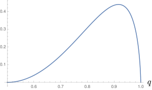
Figure 8: Plot of $[\ln\big{(}\dfrac{q}{1-q}\big{)}]^{2}q(1-q)$ as a function of $q$.

Appendix E Dynamical solution of the non-Markovian model

In this Appendix we show exact and approximate (Slow-Driving) solutions of the non-Markovian model of Section IV.1. We remind that we are interested in the analysis of the dynamics of the qubit $\mathcal{S}$ when coupled to one of the two baths, that without loss of generality can be considered to be the cold one, so that the state of the system and the ancillary qubit ${\cal{A}}_{\rm C}$ of the bath can be described by the density matrix $\hat{\mathbb{R}}_{\rm{C}}$, as well al the local states of $\mathcal{S}$ ($\hat{\rho}:=\text{Tr}_{\cal{A}_{\rm C}}[\hat{\mathbb{R}}_{\rm{C}}]$) and $\cal{A}_{\rm C}$ ($\hat{\rho}_{\rm C}:=\text{Tr}_{\cal S}[\hat{\mathbb{R}}_{\rm{C}}]$). As pictured in Fig.4 we remind the local Hamiltonians and coupling interaction

$$\hat{H}_{tot}(t)=\hat{H}_{t}+\hat{H}_{{\cal A}_{\rm C}}+\hat{V}_{\rm C}=\frac{\epsilon(t)}{2}\sigma^{z}+\frac{E_{C}}{2}\sigma^{z}_{\mathcal{A}_{\rm C}}+\gamma_{\rm C}(\sigma^{+}\otimes\sigma^{-}_{\mathcal{A}_{\rm C}}+\sigma^{-}\otimes\sigma^{+}_{\mathcal{A}_{\rm C}})\ ,$$ (128)

as well as the thermalizing dissipators

$$\mathcal{D}[\hat{\mathbb{R}}_{\rm{C}}]=\Gamma_{\rm C}(\hat{\Omega}^{(C)}_{\hat{H}_{t}}\otimes\hat{\rho}_{\rm C}-\hat{\mathbb{R}}_{\rm{C}})+\Gamma_{\mathcal{A}_{\rm C}}(\hat{\rho}\otimes\hat{\Omega}^{(C)}_{\hat{H}_{{\cal A}_{\rm C}}}-\hat{\mathbb{R}}_{\rm{C}})$$ (129)

so that in the interaction picture the dynamical equation is

$$\dot{\hat{\mathbb{R}}}_{\rm{C}}=-i\gamma_{\rm C}[e^{-i\delta t}\mathcal{\sigma}^{+}\otimes\mathcal{\sigma}_{{\cal A}_{\rm C}}^{-}+e^{i\delta t}\mathcal{\sigma}^{-}\otimes\mathcal{\sigma}_{\mathcal{A}_{\rm C}}^{+},\hat{\mathbb{R}}_{\rm{C}}]+\Gamma_{\mathcal{A}_{\rm C}}(\hat{\rho}\otimes\hat{\Omega}^{(C)}_{\hat{H}_{{\cal A}_{\rm C}}}-\hat{\mathbb{R}}_{\rm{C}})+\Gamma_{\rm C}(\hat{\rho}_{\rm C}\otimes\hat{\Omega}^{(C)}_{\hat{H}_{t}}-\hat{\mathbb{R}}_{\rm{C}})\ ,$$ (130)

with $\delta=\epsilon-E_{C}$.
Introducing the thermal ground state probabilities and a time dependent phase

$$p_{s}(t)=\frac{1}{e^{-\beta_{\rm C}\epsilon(t)}+1}\ ,\quad\quad p_{\rm C}=\frac{1}{e^{-\beta_{\rm C}E_{\rm C}}+1}\ ,\quad\quad\phi(t)=e^{i\delta t}\ ,$$ (131)

we can solve equation (130) by writing it in the computational basis $\hat{\mathbb{R}}_{\rm{C}}\equiv\sum_{\alpha,\beta,\mu,\nu=0,1}{\rho}_{\alpha\mu\beta\nu}|\alpha\rangle\!\langle\beta|_{{}_{\mathcal{A}_{\rm C}}}\otimes|\mu\rangle\!\langle\nu|_{{}_{\cal S}}\;.$ We get, in matrix form,

$$\bigg{(}\frac{d}{dt}-(\Gamma_{\rm C}+\Gamma_{{\cal A}_{C}})\mathds{1}\bigg{)}\begin{pmatrix}{\rho}_{0000}&{\rho}_{0001}&{\rho}_{0010}&{\rho}_{0011}\\ {\rho}_{0100}&{\rho}_{0101}&{\rho}_{0110}&{\rho}_{0111}\\ {\rho}_{1000}&{\rho}_{1001}&{\rho}_{1010}&{\rho}_{1011}\\ {\rho}_{1100}&{\rho}_{1101}&{\rho}_{1110}&{\rho}_{1111}\\ \end{pmatrix}=\\ \\ \left(\begin{array}[]{c|c|c|c}\Gamma_{{\cal A}_{C}}p_{\rm C}({\rho}_{{}_{0000}}\!\!+\!{\rho}_{{}_{1010}})&\Gamma_{{\cal A}_{C}}p_{\rm C}({\rho}_{{}_{0001}}\!\!+\!{\rho}_{{}_{1011}})\!\!&&\\ +\Gamma_{\rm C}p_{s}({\rho}_{{}_{0000}}\!\!+\!{\rho}_{{}_{0101}})&&\Gamma_{\rm C}p_{s}({\rho}_{{}_{0010}}\!\!+\!{\rho}_{{}_{0111}})\!\!&0\\ &+\!i\gamma_{\rm C}\phi{\rho}_{{}_{0010}}&+i\gamma_{\rm C}\phi^{*}{\rho}_{{}_{0001}}&\\ \hline\cr&\Gamma_{{\cal A}_{C}}p_{\rm C}({\rho}_{{}_{1111}}\!\!+\!{\rho}_{{}_{0101}})\!\!&&\\ \cdots&+\Gamma_{\rm C}(1-p_{s})({\rho}_{{}_{0000}}\!\!+\!{\rho}_{{}_{0101}})&&\Gamma_{\rm C}(1-p_{s})({\rho}_{{}_{0010}}\!\!+\!{\rho}_{{}_{0111}})\\ &+\!i\gamma_{\rm C}(\phi{\rho}_{{}_{0110}}\!\!-\phi^{*}\!{\rho}_{{}_{0110}}^{*})&+i\gamma_{\rm C}\phi^{*}({\rho}_{{}_{0101}}\!\!-\!{\rho}_{{}_{1010}})&-i\gamma_{\rm C}\phi^{*}{\rho}_{{}_{1011}}\\ \hline\cr&&\Gamma_{{\cal A}_{C}}(1-p_{\rm C})({\rho}_{{}_{0000}}\!\!+\!{\rho}_{{}_{1010}})\!\!&\Gamma_{{\cal A}_{C}}(1-p_{\rm C})({\rho}_{{}_{0001}}\!\!+\!{\rho}_{{}_{1011}})\!\\ \cdots&\cdots&+\Gamma_{\rm C}p_{s}({\rho}_{{}_{1111}}\!\!+\!{\rho}_{{}_{1010}})\!\!&\\ &&-\!i\gamma_{\rm C}(\phi{\rho}_{{}_{0110}}\!\!-\phi^{*}\!{\rho}_{{}_{0110}}^{*})&-\!i\gamma_{\rm C}\phi{\rho}_{{}_{0111}}\\ \hline\cr&&&\Gamma_{{\cal A}_{C}}(1-p_{\rm C})({\rho}_{{}_{1111}}\!\!+\!{\rho}_{{}_{0101}})\\ \cdots&\cdots&\cdots&+\Gamma_{\rm C}(1-p_{s})({\rho}_{{}_{1111}}\!\!+\!{\rho}_{{}_{1010}})\\ &&&\\ \end{array}\right)$$ (132)

where the inferior triangular part has been omitted to improve readability and can be filled by just noting $\hat{\mathbb{R}}_{\rm{C}}$ is hermitian. For each matrix element the 3 different lines represent the contributions from the ${\mathcal{A}_{\rm C}}$ dissipator ($\propto\Gamma_{{\cal A}_{C}}$), the $\mathcal{S}$ dissipator ($\propto\Gamma_{\rm C}$), and the Hamiltonian exchange ($\propto\gamma_{\rm C}$). Looking at the equation we can note that the time evolution generator is a sparse super-operator, which couples separately different subsets of components, namely the ones highlighted here with different colors

$$\begin{pmatrix}\hbox{\pagecolor{yellow}${\color[rgb]{0,0,1}{\rho}_{0000}}$}&{\color[rgb]{1,.5,0}{\rho}_{0001}}&{\color[rgb]{1,.5,0}{\rho}_{0010}}&{\color[rgb]{1,0,0}{\rho}_{0011}}\\ &\hbox{\pagecolor{yellow}${\color[rgb]{0,0,1}{\rho}_{0101}}$}&\hbox{\pagecolor{yellow}${\color[rgb]{0,0,1}{\rho}_{0110}}$}&{\color[rgb]{1,.5,0}{\rho}_{0111}}\\ &&\hbox{\pagecolor{yellow}${\color[rgb]{0,0,1}{\rho}_{1010}}$}&{\color[rgb]{1,.5,0}{\rho}_{1011}}\\ &&&\hbox{\pagecolor{yellow}${\color[rgb]{0,0,1}{\rho}_{1111}}$}\\ \end{pmatrix}\ .$$

Three different sets of equations can be then solved separately, but we will be interested in the Thermodynamics of the system, hence mainly the highlighted blue subset, because it contains the populations which determine thermodynamic variables (namely, the eigenstates of $\hat{H}_{t}+\hat{H}_{\mathcal{A}_{\rm C}}$). We can represent it as the vector

$$\vec{\mathbb{R}}(t)=\begin{pmatrix}q_{00}\\ q_{10}\\ q_{01}\\ q_{00}\\ k\end{pmatrix}$$ (133)

where $q_{ab}={\rho}_{abab}$ is the population of $\mathcal{S}$ in the state $b$ and ${\mathcal{A}_{\rm C}}$ in $a$, while $k\equiv{\rho}_{0110}$ is the coherence between the states $\ket{01}$ and $\ket{10}$ which are the ones interacting by the exchange Hamiltonian $V_{\rm C}$.

E.1 Resonant case $(\epsilon=E_{\rm C})$

Consider the instance in which the gaps are fixed equal $\epsilon=E_{\rm C}=E$; in this case the algebra has some simplifications; indeed

$$[\sigma^{+}\otimes\sigma^{-}_{\mathcal{A}_{\rm C}}+\sigma^{-}\otimes\sigma^{+}_{\mathcal{A}_{\rm C}}\;,\;\sigma^{z}+\sigma^{z}_{\mathcal{A}_{\rm C}}]_{-}=0$$ (134)

so that the value of the interaction Hamiltonian is conserved in absence of the dissipative dynamics (or decreases exponentially, see below). It is easy to check that the (only) stationary state is $\hat{\mathbb{R}}_{\rm{C}}=\hat{\Omega}^{(C)}_{\hat{H}_{t}}\otimes\hat{\Omega}^{(C)}_{\hat{H}_{{\cal A}_{\rm C}}}$ (or $\hat{\Omega}_{\rm C}\otimes\hat{\Omega}_{\rm C}$ for simplicity).Having the gap equal we can call

$$p_{s}\equiv p_{\rm C}\equiv p_{0}=\frac{1}{e^{-\beta_{\rm C}E_{\rm C}}+1}\ .$$ (135)

We will also write $\mathcal{L}$, with a small abuse of notation, to indicate the Lindblad generator of the dynamics restricted to the different subsets of components. The equation (132) for the vector (133) can be written in this special case as

$$\left\{\begin{aligned} \dot{q}_{00}+(\Gamma_{{\mathcal{A}_{\rm C}}}+\Gamma_{\rm C})q_{00}&=\Gamma_{{\mathcal{A}_{\rm C}}}p_{0}(q_{00}+q_{10})+\Gamma_{\rm C}p_{0}(q_{00}+q_{01})\\ \dot{q}_{01}+(\Gamma_{{\mathcal{A}_{\rm C}}}+\Gamma_{\rm C})q_{01}&=\Gamma_{{\mathcal{A}_{\rm C}}}p_{0}(q_{11}+q_{01})+\Gamma_{\rm C}(1-p_{0})(q_{00}+q_{01})+i\gamma_{\rm C}(k-k^{*})\\ \dot{q}_{10}+(\Gamma_{{\mathcal{A}_{\rm C}}}+\Gamma_{\rm C})q_{10}&=\Gamma_{{\mathcal{A}_{\rm C}}}(1-p_{0})(q_{00}+q_{10})+\Gamma_{\rm C}p_{0}(q_{11}+q_{10})-i\gamma_{\rm C}(k-k^{*})\\ \dot{q}_{11}+(\Gamma_{{\mathcal{A}_{\rm C}}}+\Gamma_{\rm C})q_{00}&=\Gamma_{{\mathcal{A}_{\rm C}}}(1-p_{0})(q_{11}+q_{01})+\Gamma_{\rm C}(1-p_{0})(q_{11}+q_{10})\\ \dot{k}+\Gamma_{{\mathcal{A}_{\rm C}}}k+\Gamma_{\rm C}k&=i\gamma_{\rm C}(q_{01}-q_{10})\\ \end{aligned}\right.\quad.$$ (136)

Note that the real part of the coherence $\Re(k)$ satisfies  $\Re(\dot{k})+\Gamma\Re(k)=0$ , hence it is decoupled from the rest and it just dies exponentially $\sim e^{-\Gamma t}$. Calling $\Im(k)\equiv I$ the system can be thus be written

$$\frac{d}{dt}\begin{pmatrix}q_{00}\\ q_{10}\\ q_{01}\\ q_{00}\\ I\end{pmatrix}=\tilde{\mathcal{L}}\begin{pmatrix}q_{00}\\ q_{10}\\ q_{01}\\ q_{00}\\ I\end{pmatrix}-(\Gamma_{\rm C}+\Gamma_{{\mathcal{A}_{\rm C}}})\begin{pmatrix}q_{00}\\ q_{10}\\ q_{01}\\ q_{00}\\ I\end{pmatrix}\ ,$$ (137)

the Lindblad generator being $\mathcal{L}=\tilde{\mathcal{L}}-(\Gamma_{\rm C}+\Gamma_{{\mathcal{A}_{\rm C}}})$ and

$$\tilde{\mathcal{L}}=\begin{pmatrix}(\Gamma_{\rm C}+\Gamma_{{\cal A}_{C}})p_{0}&\Gamma_{{\cal A}_{C}}p_{0}&\Gamma_{\rm C}p_{0}&0&0\\ \Gamma_{{\cal A}_{C}}(1-p_{0})&\Gamma_{{\cal A}_{C}}(1-p_{0})+\Gamma_{\rm C}p_{0}&0&\Gamma_{\rm C}p_{0}&+2\gamma_{\rm C}\\ \Gamma_{\rm C}(1-p_{0})&0&\Gamma_{{\cal A}_{C}}p_{0}+\Gamma_{\rm C}(1-p_{0})&\Gamma_{{\cal A}_{C}}p_{0}&-2\gamma_{\rm C}\\ 0&\Gamma_{\rm C}(1-p_{0})&\Gamma_{{\cal A}_{C}}(1-p_{0})&(\Gamma_{{\cal A}_{C}}+\Gamma_{\rm C})(1-p_{0})&0\\ 0&-\gamma_{\rm C}&+\gamma_{\rm C}&0&0\\ \end{pmatrix}\$$ (138)

which in the $\Gamma_{{\cal A}_{C}}=\Gamma_{\rm C}=\Gamma$ case becomes ($\gamma_{\rm C}^{\prime}=\gamma_{\rm C}/\Gamma$)

$$\tilde{\mathcal{L}}=\Gamma\begin{pmatrix}2p_{0}&p_{0}&p_{0}&0&0\\ (1-p_{0})&1&0&p_{0}&+2\gamma_{\rm C}^{\prime}\\ (1-p_{0})&0&1&p_{0}&-2\gamma_{\rm C}^{\prime}\\ 0&(1-p_{0})&(1-p_{0})&2(1-p_{0})&0\\ 0&-\gamma_{\rm C}^{\prime}&+\gamma_{\rm C}^{\prime}&0&0\\ \end{pmatrix}\ .$$ (139)

To solve the dynamics one can find eigenvalues and eigenvectors of such a matrix. In the $\Gamma_{\rm C}=\Gamma_{{\cal A}_{C}}$ case the particular symmetry of the problem is reflected in the tractable form of the eigensystem of $\mathcal{L}$, which is (subtracting already $-2\Gamma$ to all eigenvalues and expressing in units of $\Gamma$)

$$\lambda_{0}=0\rightarrow\vec{\rho}_{0}=\begin{pmatrix}p_{0}^{2}\\ p_{0}(1-p_{0})\\ p_{0}(1-p_{0})\\ (1-p_{0})^{2}\\ 0\end{pmatrix}\equiv\text{thermal state}\ \hat{\Omega}_{\rm C}\otimes\hat{\Omega}_{\rm C},\\ \lambda_{1}=-1\rightarrow\vec{\rho}_{1}=\begin{pmatrix}p_{0}\\ \frac{1-2p_{0}}{2}\\ \frac{1-2p_{0}}{2}\\ -(1-p_{0})\\ 0\end{pmatrix}\ ,\quad\lambda_{2}=-2\rightarrow\vec{\rho}_{2}=\begin{pmatrix}1\\ -1\\ -1\\ 1\\ 0\end{pmatrix}\ ,\\ \lambda_{3,4}=\frac{-3\pm\sqrt{1-16\gamma_{\rm C}^{\prime 2}}}{2}\rightarrow\vec{\rho}_{3,4}=\begin{pmatrix}0\\ \frac{1\pm\sqrt{1-16\gamma_{\rm C}^{\prime 2}}}{4\gamma_{\rm C}^{\prime}}\\ -\frac{1\pm\sqrt{1-16\gamma_{\rm C}^{\prime 2}}}{4\gamma_{\rm C}^{\prime}}\\ 0\\ -1\end{pmatrix}\ .$$ (140)

We can then solve completely the dynamics for an initial state of the form $\hat{\mathbb{R}}_{\rm{C}}(t_{0})=\hat{\rho}\otimes\hat{\Omega}_{\rm C}$, that is out of equilibrium on $\mathcal{S}$ and thermal on ${\mathcal{A}_{\rm C}}$, as requested by our model.
Suppose for the moment that also $\hat{\rho}$ is diagonal, that is

$$\hat{\rho}(t_{0})=\begin{pmatrix}a&0\\ 0&1-a\end{pmatrix}\Rightarrow\begin{pmatrix}q_{00}\\ q_{10}\\ q_{01}\\ q_{00}\\ I\end{pmatrix}(t_{0})=\begin{pmatrix}ap_{0}\\ a(1-p_{0})\\ (1-a)p_{0}\\ (1-a)(1-p_{0})\\ 0\end{pmatrix}\ .$$ (141)

We write $a=p_{0}+\Delta$ to quantify how much $\hat{\rho}$ is out of equilibrium. We decompose (141) as a combination of the eigenvectors (140), in order to write the solution which will be

$$\vec{q}(t)=\vec{\rho_{0}}+\Delta\vec{\rho}_{1}e^{-\Gamma t}+\frac{\Delta\gamma_{\rm C}^{\prime}}{\sqrt{1-16\gamma_{\rm C}^{\prime 2}}}(\vec{\rho}_{3}e^{\lambda_{3}t}-\vec{\rho}_{4}e^{\lambda_{4}t})\ .$$ (142)

Summing the first two components we can obtain the time-dependent ground state population of $\mathcal{S}$ ​ that is, calling $\kappa_{\rm C}=\sqrt{1-16\gamma_{\rm C}^{\prime 2}}\ ,$

$$a(t)=p_{0}+\Delta\bigg{(}\frac{1}{2}e^{-\Gamma t}+\frac{1+\kappa_{\rm C}}{4\kappa_{\rm C}}e^{-\frac{3}{2}\Gamma t+\frac{\kappa_{\rm C}}{2}\Gamma t}-\frac{1-\kappa_{\rm C}}{4\kappa_{\rm C}}e^{-\frac{3}{2}\Gamma t-\frac{\kappa_{\rm C}}{2}\Gamma t}\bigg{)}=p_{0}+\Delta f_{{\rm C}}(t)\ ,$$ (143)

having defined

$$f_{{\rm C}}(t)\equiv\frac{e^{-\Gamma t}}{2}+e^{(-\frac{3}{2}+\frac{\kappa_{\rm C}}{2})\Gamma t}\bigg{(}\frac{1+\kappa_{\rm C}}{4\kappa_{\rm C}}\bigg{)}-e^{(-\frac{3}{2}-\frac{\kappa_{\rm C}}{2})\Gamma t}\bigg{(}\frac{1-\kappa_{\rm C}}{4\kappa_{\rm C}}\bigg{)}\ .$$ (144)

E.2 Non-resonant case $(\epsilon(t)\neq E_{\rm C})$ - Slow-Driving

In case the two qubits are not resonant equation (132) for the vector (133) takes the general form

$$\left\{\begin{aligned} \dot{q}_{00}+(\Gamma_{{\cal A}_{C}}+\Gamma_{\rm C})q_{00}&=\Gamma_{{\cal A}_{C}}p_{\rm C}(q_{00}+q_{10})+\Gamma_{\rm C}p_{s}(q_{00}+q_{01})\\ \dot{q}_{01}+(\Gamma_{{\cal A}_{C}}+\Gamma_{\rm C})q_{01}&=\Gamma_{{\cal A}_{C}}p_{\rm C}(q_{11}+q_{01})+\Gamma_{\rm C}(1-p_{s})(q_{00}+q_{01})+i\gamma_{\rm C}(\phi k-\phi^{*}k^{*})\\ \dot{q}_{10}+(\Gamma_{{\cal A}_{C}}+\Gamma_{\rm C})q_{10}&=\Gamma_{{\cal A}_{C}}(1-p_{\rm C})(q_{00}+q_{10})+\Gamma_{\rm C}p_{s}(q_{11}+q_{10})-i\gamma_{\rm C}(\phi k-\phi^{*}k^{*})\\ \dot{q}_{11}+(\Gamma_{{\cal A}_{C}}+\Gamma_{\rm C})q_{00}&=\Gamma_{{\cal A}_{C}}(1-p_{\rm C})(q_{11}+q_{01})+\Gamma_{\rm C}(1-p_{s})(q_{11}+q_{10})\\ \dot{k}+\Gamma_{{\cal A}_{C}}k+\Gamma_{\rm C}k&=i\gamma_{\rm C}\phi^{*}(q_{01}-q_{10})\end{aligned}\right.\quad.$$ (145)

We note that the 2nd and 3rd equation here can be rewritten using $\hat{k}=\phi k$, which satisfies

$$\dot{\hat{k}}=\dot{\phi}k+\phi\dot{k}=i\delta\phi k+\phi(i\gamma_{\rm C}\phi^{*}(q_{01}-q_{10})-k(\Gamma_{{\cal A}_{C}}+\Gamma_{\rm C}))=i\delta\hat{k}+i\gamma_{\rm C}(q_{01}-q_{10})-(\Gamma_{{\cal A}_{C}}+\Gamma_{\rm C})\hat{k}\ .$$ (146)

In this way we can write, calling $\Im(k)\equiv I$ and $\Re(k)\equiv R$,

$$\frac{d}{dt}\begin{pmatrix}q_{00}\\ q_{01}\\ q_{10}\\ q_{00}\\ I\\ R\end{pmatrix}=\tilde{\mathcal{L}}\begin{pmatrix}q_{00}\\ q_{01}\\ q_{10}\\ q_{00}\\ I\\ R\end{pmatrix}-(\Gamma_{\rm C}+\Gamma_{{\mathcal{A}_{\rm C}}})\begin{pmatrix}q_{00}\\ q_{01}\\ q_{10}\\ q_{00}\\ I\\ R\end{pmatrix}$$ (147)

with $\mathcal{L}=\tilde{\mathcal{L}}-(\Gamma_{\rm C}+\Gamma_{{\cal A}_{C}})\mathds{1}\ ,$

$$\hat{\mathcal{L}}=\begin{pmatrix}\Gamma_{\rm C}p_{s}+\Gamma_{{\cal A}_{C}}p_{\rm C}&\Gamma_{\rm C}p_{s}&\Gamma_{{\cal A}_{C}}p_{\rm C}&0&0&0\\ \Gamma_{\rm C}(1-p_{s})&\Gamma_{{\cal A}_{C}}p_{\rm C}+\Gamma_{\rm C}(1-p_{s})&0&\Gamma_{{\cal A}_{C}}p_{\rm C}&-2\gamma_{\rm C}&0\\ \Gamma_{{\cal A}_{C}}(1-p_{\rm C})&0&\Gamma_{{\cal A}_{C}}(1-p_{\rm C})+\Gamma_{\rm C}p_{s}&\Gamma_{\rm C}p_{s}&+2\gamma_{\rm C}&0\\ 0&\Gamma_{{\cal A}_{C}}(1-p_{\rm C})&\Gamma_{\rm C}(1-p_{s})&\Gamma_{{\cal A}_{C}}(1-p_{\rm C})+\Gamma_{\rm C}(1-p_{s})&0&0\\ 0&+\gamma_{\rm C}&-\gamma_{\rm C}&0&0&\delta\\ 0&0&0&0&-\delta&0\end{pmatrix}.$$ (148)

The null eigenvector of $\mathcal{L}$ (i.e. the stationary state $\rho^{(0)}$) is not in general simply the thermal state $\Omega_{\rm C}\otimes\Omega_{\rm C}$, but it reduces to it in the limit

$$\delta\rightarrow 0\quad\quad(p_{\rm C}-p_{s}\rightarrow 0)\Rightarrow\vec{\rho}_{0}=\begin{pmatrix}p^{2}\\ p(1-p)\\ p(1-p)\\ (1-p)^{2}\\ 0\\ 0\end{pmatrix}\ .$$ (149)

At first order in $\delta$ we find

$$\vec{\rho}_{0}=\begin{pmatrix}p_{\rm C}p_{s}\\ p_{\rm C}(1-p_{s})\\ p_{s}(1-p_{\rm C})\\ (1-p_{\rm C})(1-p_{s})\\ 0\\ 0\end{pmatrix}-\dfrac{\Delta_{p}}{N}\begin{pmatrix}2\gamma_{\rm C}^{2}(\Gamma_{{\cal A}_{C}}p_{\rm C}-\Gamma_{\rm C}p_{s})\\ 2\gamma_{\rm C}^{2}((\Gamma_{\rm C}p_{s}-\Gamma_{{\cal A}_{C}}p_{\rm C})-\Gamma_{\rm C})\\ 2\gamma_{\rm C}^{2}((\Gamma_{\rm C}p_{s}-\Gamma_{{\cal A}_{C}}p_{\rm C})+\Gamma_{{\cal A}_{C}})\\ 2\gamma_{\rm C}^{2}(\Gamma_{{\cal A}_{C}}(p_{\rm C}-1)-\Gamma_{\rm C}(p_{s}-1))\\ -\Gamma_{\rm C}\Gamma_{{\cal A}_{C}}\gamma_{\rm C}\\ 0\end{pmatrix}\ ,$$ (150)

the normalization being $N=(\Gamma_{\rm C}\Gamma_{{\cal A}_{C}}+2\gamma_{\rm C}^{2})(\Gamma_{\rm C}+\Gamma_{{\cal A}_{C}})\ .$ Note that in both approximations the real part of the coherence $\Re(\rho_{{}_{0110}})=[\vec{\rho}_{0}]_{6}=0$ is null; this allows us to neglect work contribution in the contacts and detachments from the baths, as in the resonant case.

Following the approach described in Section II.3 we can now compute the first order correction in Slow-Driving to the dynamics. Looking at the formal solution of the S-D technique (16) we need for the computation:

• the quasi-static solution $\hat{\rho}^{(0)}$ found in (150),

• the dynamics generator $\mathcal{L}$ we wrote explicitly,

• the projector on the null-trace subspace $\mathcal{P}$.

This last operator is easily found. The trace of the state is given from the sum of the 4 populations

$$\text{Tr}[\hat{\mathbb{R}}_{\rm{C}}]=q_{00}+q_{01}+q_{10}+q_{11}\ .$$ (151)

In order to project on the null-trace subspace we have to subtract to each population $\text{Tr}[\rho]/4$, that is $q_{ij}\rightarrow q_{ij}-\frac{1}{4}\sum_{a,b}q_{ab}$, while the coherences stay unchanged. This can be written as

$$\begin{pmatrix}q_{00}\\ q_{01}\\ q_{10}\\ q_{11}\\ I\\ R\end{pmatrix}\rightarrow\begin{pmatrix}q_{00}\\ q_{01}\\ q_{10}\\ q_{11}\\ I\\ R\end{pmatrix}-\frac{1}{4}\begin{pmatrix}1&1&1&1&0&0\\ 1&1&1&1&0&0\\ 1&1&1&1&0&0\\ 1&1&1&1&0&0\\ 0&0&0&0&0&0\\ 0&0&0&0&0&0\\ \end{pmatrix}\begin{pmatrix}q_{00}\\ q_{01}\\ q_{10}\\ q_{11}\\ I\\ R\end{pmatrix}\ ,\qquad\text{i.e.}\qquad\mathcal{P}=\begin{pmatrix}\frac{3}{4}&-\frac{1}{4}&-\frac{1}{4}&-\frac{1}{4}&0&0\\ -\frac{1}{4}&\frac{3}{4}&-\frac{1}{4}&-\frac{1}{4}&0&0\\ -\frac{1}{4}&-\frac{1}{4}&\frac{3}{4}&-\frac{1}{4}&0&0\\ -\frac{1}{4}&-\frac{1}{4}&-\frac{1}{4}&\frac{3}{4}&0&0\\ 0&0&0&0&1&0\\ 0&0&0&0&0&1\\ \end{pmatrix}\ .$$ (152)

Now we have all the ingredients to compute (with the help of Wolfram Mathematica) the first correction $\vec{\rho}_{1}=(\mathcal{LP})^{-1}\dot{\vec{\rho}}_{0}\$. The resulting expression is too complicated to be reported here, however, it is possible to compute the correction to the ground state population of $\mathcal{S}$ ​, $q_{00}^{(1)}+q_{10}^{(1)}$, which is in the form

$$q_{00}^{(1)}+q_{10}^{(1)}=[\rho_{s}^{(1)}]_{00}=-\dot{p}_{s}A_{\rm C}\ ,$$ (153)

with an amplitude $A_{\rm C}$ that admits a closed but unfortunately still very convoluted general expression, which for the sake of readability we do not report here in its full extension. Nevertheless, in the resonance ($\epsilon=E_{\rm C}$) limit we considered for our model we find

$$\delta=0\Rightarrow A_{\rm C}=\frac{\Gamma_{\rm C}((\Gamma_{{\cal A}_{C}}^{2}+\Gamma_{{\cal A}_{C}}\Gamma_{\rm C})^{2}+2\gamma_{\rm C}^{2}(\Gamma_{{\cal A}_{C}}^{2}+2\Gamma_{{\cal A}_{C}}\Gamma_{\rm C}+4\gamma_{\rm C}^{2})}{(\Gamma_{{\cal A}_{C}}+\Gamma_{\rm C})^{2}(\Gamma_{{\cal A}_{C}}\Gamma_{\rm C}+2\gamma_{\rm C}^{2})^{2}}\ .$$ (154)

Appendix F Non-Markovian character of the dynamics

Here we show that the model of Sec. IV has an explicit non-Markovian character which depends on the non zero value of the parameters $\gamma_{j}$ that gauge the coupling between $\mathcal{S}$ and the ancillas ${\cal A}_{j}$. For this task, given two input states $\hat{\rho}^{(1)}(0)$, $\hat{\rho}^{(2)}(0)$ of ${\cal S}$ and $\hat{\rho}^{(1)}(t)$, $\hat{\rho}^{(2)}(t)$ their corresponding dynamical evolutions under the action of the model, we consider the information-backflow BLP quantity (Breuer et al., 2016)

$$\mathcal{N}_{BLP}(\hat{\rho}^{(1)}(0),\hat{\rho}^{(2)}(0)):=\int dt\;\dot{D}(\hat{\rho}^{(1)}(t),\hat{\rho}^{(2)}(t))\;\Theta[\dot{D}(\hat{\rho}^{(1)}(t),\hat{\rho}^{(2)}(t))]\ ,$$ (155)

with $\Theta$ being the Heaviside function that restrict the domain of integration to the one where the integrand is positive, and where $D(\hat{\rho}^{(1)}(t),\hat{\rho}^{(2)}(t)):=\frac{1}{2}||\hat{\rho}^{(1)}(t)-\hat{\rho}^{(2)}(t)||_{1}$ is the trace distance Holevo (2012). As discussed in Ref. (Breuer et al., 2016) value of $\mathcal{N}_{BLP}(\hat{\rho}^{(1)}(0),\hat{\rho}^{(2)}(0))$ greater then zero would imply non-Markovian character of the dynamics.

In our case, focusing only at $\hat{\rho}^{(1)}(0)$, $\hat{\rho}^{(2)}(0)$ having no coherence terms, we can simplify the analysis exploiting the fact that $D(\rho^{(1)}(t),\rho^{(2)}(t))=|p^{(1)}(t)-p^{(2)}(t)|$, where for $j=1,2$, $p^{(j)}(t)$ is the ground state population of the $\hat{\rho}^{(j)}(t)$. On-resonance ($\epsilon=E_{j}$) the solutions given in Sec. E.1 yields, in adimensional units ($\Gamma_{j}=1$),

$$\frac{p^{(1)}(t)-p^{(2)}(t)}{p^{(1)}(0)-p^{(2)}(0)}=-\frac{e^{-t/2}}{2}-\frac{3}{8}e^{-\frac{3}{2}t}\bigg{(}(1+\frac{1}{\kappa_{j}})e^{\kappa_{j}t}+(1-\frac{1}{\kappa_{j}})e^{-\kappa_{j}t}\bigg{)}+\frac{1}{4}e^{-\frac{3}{2}t}\bigg{(}(1+\kappa_{j})e^{\kappa_{j}t}+(1-\kappa_{j})e^{-\kappa_{j}t}\bigg{)}\;,$$ (156)

where $\kappa_{j}=\sqrt{1-16(\gamma_{j}/\Gamma_{j})^{2}}$ . Replacing this into (155) and performing the integration numerically we obtain the results reported in Fig.  9 as function of $y_{j}=\gamma_{j}/\Gamma_{j}$. As expected, the non-Markovianity is monotonously increasing with $\gamma_{j}$. Also, we find a threshold value under which this particular non-Markovianity witness is null.

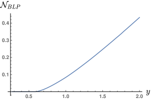
Figure 9: The non-Markovian measure $\mathcal{N}_{BLP}$ as a function of $y_{j}$.

Appendix G Symmetric Otto cycle has maximum power for $\tau_{\rm H}=\tau_{\rm C}$

In this appendix we prove that the power expressed by Eq. (72) is maximized, in case the coupling to the two baths is symmetric (i.e. $f_{\rm H}(t)=f_{\rm C}(t):=f(t)$ in Eq. (72)), by choosing the time durations $\tau_{\rm H}=\tau_{\rm C}$ equal. In fact under this assumption the power can be written as

$$P=(\epsilon_{2}-\epsilon_{1})(p_{\rm C}-p_{\rm H})\dfrac{\big{(}1-f(\tau_{\rm H})\big{)}\big{(}1-f(\tau_{\rm C})\big{)}}{\big{(}\tau_{\rm C}+\tau_{\rm H}\big{)}\big{(}1-f(\tau_{\rm C})f(\tau_{\rm H})\big{)}}:=(\epsilon_{2}-\epsilon_{1})(p_{\rm C}-p_{\rm H})C(\tau_{\rm C},\tau_{\rm H})\;.$$ (157)

We show that when $\tau_{\rm H}\neq\tau_{\rm C}$ at least one between $C(\tau_{\rm C},\tau_{\rm C})$ and $C(\tau_{\rm H},\tau_{\rm H})$ is greater than $C(\tau_{\rm C},\tau_{\rm H})$, meaning that $\{\tau_{\rm H},\tau_{\rm C}\}$ would be outperformed by one of the two choices. To prove it we demonstrate that $C(\tau_{\rm C},\tau_{\rm H})\leq\sqrt{C(\tau_{\rm C},\tau_{\rm C})C(\tau_{\rm H},\tau_{\rm H})}$, which implies the thesis. This is equivalent to verify the following inequality holds

$$\frac{(1-f(\tau_{\rm C}))(1-f(\tau_{\rm H}))}{(1-f(\tau_{\rm C})f(\tau_{\rm H}))(\tau_{\rm C}+\tau_{\rm H})}\leq\sqrt{\frac{(1-f(\tau_{\rm C}))^{2}}{(1-f^{2}(\tau_{\rm C}))2\tau_{\rm C}}\frac{(1-f(\tau_{\rm H}))^{2}}{(1-f^{2}(\tau_{\rm H}))2\tau_{\rm H}}}\ ,$$ (158)

which is true by noting the numerator is the same and on the denominator by direct inspection

$$\tau_{\rm C}+\tau_{\rm H}\geq 2\sqrt{\tau_{\rm C}\tau_{\rm H}}\ ,$$ (159)

$$(1-f(\tau_{\rm C})f(\tau_{\rm H}))\geq\sqrt{(1-f^{2}(\tau_{\rm C}))(1-f^{2}(\tau_{\rm H}))}\ .$$ (160)

References

- Gemmer et al. (2009) J. Gemmer, M. Michel, and G. Mahler, Quantum Thermodynamics: Emergence of Thermodynamic Behavior Within Composite Quantum Systems, Lecture Notes in Physics (Springer Berlin Heidelberg, 2009).
- Goold et al. (2016) J. Goold, M. Huber, A. Riera, L. del Rio, and P. Skrzypczyk, Journal of Physics A: Mathematical and Theoretical 49, 143001 (2016).
- Vinjanampathy and Anders (2016) S. Vinjanampathy and J. Anders, Contemporary Physics 57, 545 (2016).
- Linden et al. (2010) N. Linden, S. Popescu, and P. Skrzypczyk, Physical Review Letters 105, 130401 (2010).
- Skrzypczyk et al. (2011) P. Skrzypczyk, N. Brunner, N. Linden, and S. Popescu, Journal of Physics A: Mathematical and Theoretical 44, 492002 (2011).
- Koski et al. (2014) J. V. Koski, V. F. Maisi, J. P. Pekola, and D. V. Averin, Proceedings of the National Academy of Sciences 111, 13786 (2014).
- Pekola (2015) J. P. Pekola, Nature Physics 11, 118 (2015).
- Batalhão et al. (2014) T. B. Batalhão, A. M. Souza, L. Mazzola, R. Auccaise, R. S. Sarthour, I. S. Oliveira, J. Goold, G. De Chiara, M. Paternostro, and R. M. Serra, Physical Review Letters 113, 140601 (2014).
- An et al. (2015) S. An, J.-N. Zhang, M. Um, D. Lv, Y. Lu, J. Zhang, Z.-Q. Yin, H. Quan, and K. Kim, Nature Physics 11, 193 (2015).
- Roßnagel et al. (2016) J. Roßnagel, S. T. Dawkins, K. N. Tolazzi, O. Abah, E. Lutz, F. Schmidt-Kaler, and K. Singer, Science 352, 325 (2016).
- Zhang et al. (2014a) K. Zhang, F. Bariani, and P. Meystre, Physical Review Letters 112, 150602 (2014a).
- Abah et al. (2012) O. Abah, J. Rossnagel, G. Jacob, S. Deffner, F. Schmidt-Kaler, K. Singer, and E. Lutz, Physical review letters 109, 203006 (2012).
- Ronzani et al. (2018) A. Ronzani, B. Karimi, J. Senior, Y.-C. Chang, J. T. Peltonen, C. Chen, and J. P. Pekola, Nature Physics 14, 991 (2018).
- Chen (1994) J. Chen, Journal of Physics D: Applied Physics 27, 1144 (1994).
- Rezek and Kosloff (2006) Y. Rezek and R. Kosloff, New Journal of Physics 8, 83 (2006).
- Watanabe et al. (2017) G. Watanabe, B. P. Venkatesh, P. Talkner, and A. del Campo, Physical Review Letters 118, 050601 (2017).
- Scully et al. (2011) M. O. Scully, K. R. Chapin, K. E. Dorfman, M. B. Kim, and A. Svidzinsky, Proceedings of the National Academy of Sciences 108, 15097 (2011).
- Correa et al. (2013) L. A. Correa, J. P. Palao, G. Adesso, and D. Alonso, Physical Review E 87, 042131 (2013).
- Dorfman et al. (2013) K. E. Dorfman, D. V. Voronine, S. Mukamel, and M. O. Scully, Proceedings of the National Academy of Sciences 110, 2746 (2013).
- Brunner et al. (2014) N. Brunner, M. Huber, N. Linden, S. Popescu, R. Silva, and P. Skrzypczyk, Physical Review E 89, 032115 (2014).
- Campisi and Fazio (2016) M. Campisi and R. Fazio, Nature Communications 7, 11895 (2016).
- Brandner et al. (2017) K. Brandner, M. Bauer, and U. Seifert, Physical Review Letters 119, 170602 (2017).
- Breuer and Petruccione (2002) H.-P. Breuer and F. Petruccione, The theory of open quantum systems (Oxford University Press on Demand, 2002).
- Rivas et al. (2014) A. Rivas, S. F. Huelga, and M. B. Plenio, Reports on Progress in Physics 77, 094001 (2014).
- Breuer et al. (2016) H.-P. Breuer, E.-M. Laine, J. Piilo, and B. Vacchini, Reviews of Modern Physics 88, 021002 (2016).
- Rivas et al. (2010) A. Rivas, S. F. Huelga, and M. B. Plenio, Physical Review Letters 105, 050403 (2010).
- Gorini et al. (1976) V. Gorini, A. Kossakowski, and E. C. G. Sudarshan, Journal of Mathematical Physics 17, 821 (1976).
- Lindblad (1976) G. Lindblad, Communications in Mathematical Physics 48, 119 (1976).
- Bhattacharya et al. (2018) S. Bhattacharya, B. Bhattacharya, and A. Majumdar, arXiv preprint arXiv:1803.06881 (2018).
- Bylicka et al. (2016) B. Bylicka, M. Tukiainen, D. Chruściński, J. Piilo, and S. Maniscalco, Scientific reports 6, 27989 (2016).
- Mirkin et al. (2017) N. Mirkin, P. Poggi, and D. Wisniacki, arXiv preprint arXiv:1711.10551 (2017).
- Mukherjee et al. (2015) V. Mukherjee, V. Giovannetti, R. Fazio, S. F. Huelga, T. Calarco, and S. Montangero, New Journal of Physics 17, 063031 (2015).
- Raja et al. (2018) S. H. Raja, M. Borrelli, R. Schmidt, J. P. Pekola, and S. Maniscalco, Physical Review A 97, 032133 (2018).
- Reich et al. (2015) D. M. Reich, N. Katz, and C. P. Koch, Scientific Reports 5, 12430 (2015).
- Thomas et al. (2018) G. Thomas, N. Siddharth, S. Banerjee, and S. Ghosh, arXiv preprint arXiv:1801.00744 (2018).
- Zhang et al. (2014b) X. Zhang, X. Huang, and X. Yi, Journal of Physics A: Mathematical and Theoretical 47, 455002 (2014b).
- Basilewitsch et al. (2017) D. Basilewitsch, R. Schmidt, D. Sugny, S. Maniscalco, and C. P. Koch, New Journal of Physics 19, 113042 (2017).
- Pezzutto et al. (2018) M. Pezzutto, M. Paternostro, and Y. Omar, Quantum Science and Technology (2018).
- Quan et al. (2007) H. Quan, Y. Liu, C. Sun, and F. Nori, Physical Review E 76, 031105 (2007).
- Karimi and Pekola (2016) B. Karimi and J. Pekola, Physical Review B 94, 184503 (2016).
- Kosloff and Rezek (2017) R. Kosloff and Y. Rezek, Entropy 19, 136 (2017).
- Cavina et al. (2017a) V. Cavina, A. Mari, and V. Giovannetti, Physical Review Letters 119, 050601 (2017a).
- Cavina et al. (2017b) V. Cavina, A. Mari, A. Carlini, and V. Giovannetti, arXiv preprint arXiv:1709.07400 (2017b).
- Gardiner et al. (2004) C. Gardiner, P. Zoller, and P. Zoller, Quantum noise: a handbook of Markovian and non-Markovian quantum stochastic methods with applications to quantum optics, Vol. 56 (Springer Science & Business Media, 2004).
- Esposito et al. (2010) M. Esposito, R. Kawai, K. Lindenberg, and C. Van den Broeck, Physical Review Letters 105, 150603 (2010).
- Alicki (1979) R. Alicki, Journal of Physics A: Mathematical and General 12, L103 (1979).
- Anders and Giovannetti (2013) J. Anders and V. Giovannetti, New Journal of Physics 15, 033022 (2013).
- Kieu (2004) T. D. Kieu, Phys. Rev. Lett. 93, 140403 (2004).
- Parrondo et al. (2015) J. M. Parrondo, J. M. Horowitz, and T. Sagawa, Nature Physics 11, 131 (2015).
- Esposito and den Broeck (2011) M. Esposito and C. V. den Broeck, EPL (Europhysics Letters) 95, 40004 (2011).
- Holevo (2012) A. S. Holevo, Quantum systems, channels, information: a mathematical introduction, Vol. 16 (Walter de Gruyter, 2012).
- Andresen et al. (1984) B. Andresen, R. S. Berry, M. J. Ondrechen, and P. Salamon, Accounts of Chemical Research 17, 266 (1984).
- Curzon and Ahlborn (1975) F. L. Curzon and B. Ahlborn, American Journal of Physics 43, 22 (1975).
- (54) P. Abiuso and M. Perarnau, Work in preparation.
- Erdman et al. (2018) P. A. Erdman, V. Cavina, R. Fazio, F. Taddei, and V. Giovannetti, arXiv preprint arXiv:1812.05089 (2018).
- Wilming et al. (2016) H. Wilming, R. Gallego, and J. Eisert, Physical Review E 93, 042126 (2016).
- Lekscha et al. (2018) J. Lekscha, H. Wilming, J. Eisert, and R. Gallego, Physical Review E 97, 022142 (2018).
- Perarnau-Llobet et al. (2018) M. Perarnau-Llobet, H. Wilming, A. Riera, R. Gallego, and J. Eisert, Physical Review Letters 120, 120602 (2018).
- (59) This condition can be always guaranteed also when considering systems strongly out-of equilibrium (e.g. for the Otto cycle case) assuming a sufficient number of ancillary systems () sequentially interacting with and relaxing afterwards.
- Scandi and Perarnau-Llobet (2018) M. Scandi and M. Perarnau-Llobet, arXiv preprint arXiv:1810.05583 (2018).
- Ma et al. (2018) Y.-H. Ma, D.-Z. Xu, H. Dong, and C.-P. Sun, arXiv preprint arXiv:1802.09806 (2018).
- Cavina et al. (2018) V. Cavina, A. Mari, and V. Giovannetti, Proceedings of IQIS Conference 2018 (2018).