Spin bath dynamics and dynamical Renormalization Group

Abstract

We discuss the quantum dynamics of the central spin model in a regime where the central spin and bath are slaved to each other. The exact solution is found when the bath is static, and is compared with the effect of an external field, finding that they are inequivalent due to the quantum nature of the environment. When the bath has dynamics, we analyze the differences between the numerical simulation using time-dependent perturbation theory and the equation of motion technique, which shows better accuracy. We demonstrate that the use of dynamical Renormalization Group (dRG), simultaneously with the equation of motion technique, provides a suitable analytical tool to understand the physics, to capture the main physical processes, and a powerful method to eliminate secular terms. In addition, this approach allows to separate classical non-linear behavior from corrections due to quantum correlations.

I Introduction

During the last decade, a growing interest in the understanding of dynamical quantum systems has emerged. Motivated from both, theory and experiment, a whole new area of physics is being developed, where quantum systems and their dynamics play a dominant role. While non-interacting systems are quite well understood, interacting systems can display exotic new physics such as Floquet phases(FloquetTI, ; FFCI, ; ObservationFTI, ), time crystals(Time-Crystal-Wilczek, ; Time-Crystals-Review, ), many-body localization(Many-Body-Loc1, ; Many-Body-Loc2, ) and complex dynamics(SpinBathSimulations, ; UnconventionalRates, ). While the simulation of classical complex systems with non-linearities can be challenging (weather forecast, stock-market predictions, social behavior or swarming), an extra difficulty arises in quantum systems, due to the presence of entanglement.

The central spin model is one of the canonical models to study the dynamics of quantum interacting systems(TheoryBathSpin2000, ). It describes a quantum spin interacting with a set of localized modes, and can mimic molecular magnets interacting with impurities(MolecularMagnetsDecoherence, ), flux qubits coupled to electric dipoles(MartinisSQUID, ) and many other effective two-level systems interacting with localized modes. Interestingly, the dynamics in this model can be quite complex, as it is known that the localized nature of these modes requires a non-perturbative analysis and gives rise to a rich dynamical behavior(Crossover, ), which can be quite different from the spin-boson model(SpinBosonModel, ). For example, in some regimes the bath dynamics is slaved to the motion of the central spin, and the memory of the bath becomes important. This is typically discussed in terms of the dimensionless parameter $\left|A_{i}\right|/\left|\vec{\Delta}\right|$, where $A_{i}$ denotes the coupling strength between the central system and the i-th bath spin, and $\vec{\Delta}$ is the external field that gives free dynamics to the bath spins(TheoryBathSpin2000, ). Therefore, if the coupling between the two systems dominates over the free Hamiltonian for the bath $\left|A_{i}\right|/\left|\vec{\Delta}\right|\gg 1$, the dynamics of the two systems is highly correlated.

In this work we study the dynamics of the central spin model in the regime where the dynamics of the central spin and bath are slaved to each other. First, we exactly solve the case of a static bath and demonstrate that the spin bath is not equivalent to an external magnetic field, specially when the bath is not in its ground state. This leads to a damping of coherent oscillations at short times, which can be confused with decoherence (however, in this case entanglement between the two systems is not formed and it is purely a dephasing effect, which can be reversed using spin echo). Then we discuss the regime where the bath is dynamical, and the new mechanisms which can modify the coherent oscillations at different time-scales. In particular, we show how non-perturbative contributions from many-body effects lead to instanton-like transitions in the central spin, and to a suppression of the coherent oscillations due to the formation of correlations with the bath. These mechanisms appear at very different time-scales and can be captured numerically and analytically. This is possible due to the use of dynamical Renormalization Group (dRG), which allows for a natural time-scale separation, when combined with the equation of motion technique.

II Model

We consider the next Hamiltonian describing a two-level system (or qubit) interacting with a bath of spins $\vec{I}_{i}$ of arbitrary spin value $P_{i}$:

$$H = H_{0}+V_{B}$$ (1)

being

$$H_{0} = -B_{z}S^{z}-B_{\perp}S^{x}-\sum_{i=1}^{N}\left(\Delta_{z}-S^{z}A_{i}\right)I_{i}^{z}$$ (2)

$$V_{B} = -\sum_{i=1}^{N}\Delta_{\perp}I_{i}^{x}$$ (3)

We have assumed that the interaction is purely longitudinal (typically due to a large crystal field anisotropy), and that the central spin and bath spins couple, in addition to the longitudinal fields $B_{z}$ and $\Delta_{z}$, to the transverse fields $B_{\perp}$ and $\Delta_{\perp}$, respectively.

If the interaction $A_{i}$ dominates, the central spin couples to a longitudinal Overhauser field produced by the bath (it can be experimentally quite large, as $A_{i}$ does not scale as $N^{-1/2}$, which would be the case for delocalized modes), while each bath mode couples to a weaker field, produced by the central spin only. When the transverse fields are added, bath and central spin precess at different rates, and spin-flip transitions can happen, mediated by the interaction. Different Hamiltonians with more general couplings can also be studied using this formalism, but Eq.1 has the necessary ingredients to produce interesting effects and simple analytical expressions.

III Exact solution for a static bath

For $\Delta_{\perp}=0$ the Hamiltonian reduces to $H_{0}$ in Eq.1, and in this case, the model can be exactly solved and displays interesting features. In order to find the solution, it is useful to consider the many-body basis $|M;\vec{P},\vec{m}\rangle$, with $M=\pm 1/2$ labeling the two states of the central spin, and where $\vec{P}=\left(P_{1},\ldots,P_{N}\right)$ and $\vec{m}=\left(m_{1},\ldots,m_{N}\right)$ are $N$-dimensional vectors labeling the values of the bath spins at the different sites and their projection onto the z-axis, respectively. The calculation of the magnetization is straightforward because the system becomes block-diagonal for different spin bath configurations $\vec{m}$. For example, the time evolution of the longitudinal magnetization, assuming that initially the central spin is in an eigenstate of $S^{z}$, yields (full expression and derivation in the Appendix):

$$S^{z}\left(t\right)=\sum_{\vec{P},\vec{m}}S_{\vec{m}}^{z}\left(1+B_{\perp}^{2}\frac{\cos\left(\Omega_{\vec{m}}t\right)-1}{\Omega_{\vec{m}}^{2}}\right)$$ (4)

where we have defined the central spin frequency for a given bath configuration $\vec{m}$ as:

$$\Omega_{\vec{m}}=\sqrt{B_{\perp}^{2}+\left(B_{z}-\vec{A}\cdot\vec{m}\right)^{2}}$$ (5)

and $S_{\vec{m}}^{z}=\sum_{M}M|M;\vec{P},\vec{m}\rangle\langle M;\vec{P},\vec{m}|$ is the $S^{z}$ operator for the bath configuration $\vec{m}$.

Eq.4 has very interesting features, some of which have been discussed in (Zurek-SpinBath2005, ). In this case, the expression applies for arbitrary bath spin values $P_{i}$ and to any initial state configuration (e.g., this expression can be applied if the spin bath contains different nuclear isotopes). The main feature is the summation over all spin bath configurations $\sum_{\vec{P},\vec{m}}$ which can radically modify the central spin dynamics, depending on the initial condition for the bath. In this case, the initial state preparation becomes quite relevant for the subsequent dynamics.

When the bath is at low temperature $T\ll\left|A_{i}\right|$, $\left|\vec{\Delta}\right|$, mostly the ground state will be occupied and the summation over bath configurations reduces to a single term which has a shifted Zeeman splitting $B_{z}\rightarrow B_{z}-\vec{A}\cdot\vec{m}$. On the other hand, for many experimental setups the interaction with each spin is weak, and although the central spin will be at low temperature, the bath will be in the high temperature regime $\left|\vec{B}\right|\gg T\gg\left|A_{i}\right|$, $\left|\vec{\Delta}\right|$. This implies that almost all hyperfine levels will be equally occupied, and the sum over bath configurations has many terms, where each of them contributes with a different frequency $\Omega_{\vec{m}}$. In this case, although the system has a Poincare recurrence time at long times $\tau_{rec}\sim\left|A_{i}\right|^{-1}$, the dynamics resembles a “decoherence” process due to the bath. In many cases, the hyperfine levels are close to each other and broadening is large enough as to make them overlap. Then, one can approximate the sum over bath configurations by an integral with a density of states $J\left(\alpha\right)=\sum_{\vec{m},\vec{P}}\delta\left(\alpha-B_{z}+\vec{A}\cdot\vec{m}\right)$, and calculate its contribution using a stationary phase approximation. This transforms Eq.4 into:

$$S^{z}\left(t\right)\simeq S^{z}\left(1+B_{\perp}^{2}\int_{-\infty}^{\infty}J\left(\alpha\right)\frac{\cos\left(\Omega_{\alpha}t\right)-1}{\Omega_{\alpha}^{2}}d\alpha\right)$$ (6)

where we have defined $\Omega_{\alpha}=\sqrt{B_{\perp}^{2}+\alpha^{2}}$, and the spectral function is given by:

$$J\left(\alpha\right) = \frac{e^{-\frac{\left(\alpha-B_{z}\right)^{2}}{2\sigma^{2}}}}{\sqrt{2\pi\sigma^{2}}},\ \sigma=\sqrt{\frac{1}{6}\sum_{i}A_{i}^{2}P_{i}^{2}\frac{P_{i}+4}{P_{i}+2}}$$ (7)

for the case of large $P_{i}$ bath spins. The assumption of large $P_{i}$ is not required, but simplifies the expressions (the general case is analyzed in the Appendix).

Then, the dynamics is governed by a Gaussian distribution peaked at $B_{z}$, which broadens with the number of bath spins as $N^{1/2}$, and linearly with $A_{i}$ and $P_{i}$. Importantly, this happens even for the case of ordered couplings $A_{i}=A$, indicating that it is purely a bath effect, and not a disorder average. Fig.1 shows a comparison between the free dynamics and the case with a spin bath for different values of $\sigma$.

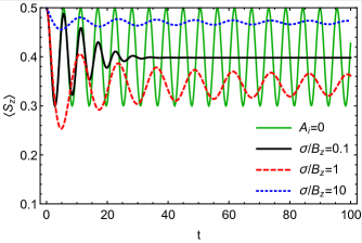
Figure 1: Comparison between the free dynamics and the case with a bath of spins for different spectral functions $J\left(\alpha\right)$ characterized by $\sigma$. We have chosen $B_{\perp}/B_{z}=0.5$ and an initial spin up state.

It shows that the coherent oscillations produced by the transverse field are damped due to a phase interference between the different bath configurations. Furthermore, the bath controls both, the damping of the oscillations and the average value of the longitudinal magnetization.

It is important to realize that the reason why the coherent oscillations are suppressed is because the bath does not act as a classical magnetic field, and its quantum nature allows different bath configurations to evolve with different phases, resulting in the suppression of coherent oscillations. Interestingly, when the width of the bath distribution $\sigma$ is of the order of the splitting $B_{z}$, the coherent oscillations remain for a long time. This shows that by tuning $B_{z}$ one can minimize the effect of the bath, or by studying the time evolution as a function of $B_{z}$, extract information about the density of states (DOS) of the environment.

IV Dynamical bath

When the bath couples to a transverse field ($\Delta_{\perp}\neq 0$), the longitudinal magnetization for the bath becomes time-dependent as well. This makes both systems precess at different rates, as typically the central spin dynamics is much faster. However, as their time evolution is not independent, a resonance can happen at longer time-scales, and produce substantial changes in the dynamics of the central spin. This is shown in Fig.2, where we have calculated the exact time-evolution for the longitudinal magnetization of the central spin, for an initially fully polarized bath (with this initial condition the previously discussed “false decoherence”, induced by the sum over bath configurations, is absent. Therefore, all changes are a consequence of the bath dynamics). The black line shows the static bath case ($\Delta_{\perp}=0$), and the red line shows the case with a small transverse field ($\Delta_{\perp}/B_{\perp}\ll 1$). When the bath is static, the central spin coherently oscillates with amplitude proportional to $B_{\perp}/\left(B_{z}-\vec{A}\cdot\vec{m}\right)$ and frequency $\Omega_{\vec{m}}$; however, when the bath is dynamical two main effects can happen at different time scales:

1. The amplitude of the oscillations gets damped at short time-scales.

2. The central spin magnetization flips at long time-scales.

The first effect is a consequence of the formation of entanglement between the central spin and the bath spins, while the second effect is produced due to a resonance between the central spin and the bath.

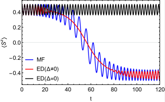
Figure 2: Comparison between the exact dynamics for $\Delta_{\perp}/B_{\perp}=0$ (black) and $\Delta_{\perp}/B_{\perp}=0.03$ (red), for the case of homogeneous couplings $A/B_{\perp}=0.05$, $N=100$ and $B_{z}=\Delta_{z}=0$. The dynamics of the bath spins, produced by $\Delta_{\perp}\neq 0$, leads to instanton-like transitions in the central spin at long time-scales, when $N\gg 1$ (this transition gets more abrupt as $N$ increases). (Blue) Numerical solution of the mean field equations. When $\Delta_{\perp}/B_{\perp}\ll 1$ the short time dynamics is identical to the case $\Delta_{\perp}=0$, with a static bath. The initial condition is a product state with central spin up and all bath spins up.

IV.1 Perturbation theory

As a first approach, let us consider time-dependent perturbation theory around the unperturbed solution (i.e., for a static bath with $\Delta_{\perp}=0$). A general state $|\Psi\left(t\right)\rangle$ can be expressed in this basis as:

$$|\Psi\left(t\right)\rangle=\sum_{M,\vec{P},\vec{m}}c_{M,\vec{P},\vec{m}}\left(t\right)e^{-itE_{\vec{m}}^{M}}|M,\vec{P},\vec{m}\rangle$$ (8)

where $H_{0}|M,\vec{P},\vec{m}\rangle=E_{\vec{m}}^{M}|M,\vec{P},\vec{m}\rangle$ and

$$E_{\vec{m}}^{M}=-\Delta_{z}\sum_{i}m_{i}+M\Omega_{\vec{m}}$$ (9)

From the time-dependent Schrödinger equation one finds that the time evolution is given by:

$$\dot{c}_{M,\vec{m}}\left(t\right)=-i\sum_{\vec{m}^{\prime}}c_{M,\vec{m}^{\prime}}\left(t\right)e^{-it\left(E_{\vec{m}^{\prime}}^{M}-E_{\vec{m}}^{M}\right)}\langle\vec{m}|V_{B}|\vec{m}^{\prime}\rangle$$ (10)

where we have used that $V_{B}$ does not change the central spin state $M$ or the bath spin $\vec{P}$. The matrix elements can be calculated straightforwardly:

$$\langle\vec{m}|V_{B}|\vec{m}^{\prime}\rangle=-\frac{\Delta_{\perp}}{2}\sum_{i=1}^{N}\left(\gamma_{P_{i},m_{i}^{\prime}}\delta_{\vec{m}-1_{i},\vec{m}^{\prime}}+\gamma_{P_{i},m_{i}}\delta_{\vec{m}+1_{i},\vec{m}^{\prime}}\right)$$ (11)

where

$$\gamma_{P_{i},m_{i}}=\sqrt{P_{i}\left(P_{i}+1\right)-m_{i}\left(m_{i}+1\right)}$$ (12)

and $\vec{m}\pm 1_{i}$ in $\delta_{\vec{m}\pm 1_{i},\vec{m}^{\prime}}$ corresponds to the bath configuration $\vec{m}$ with the bath spin at the $i$-th site changed by a unit.

For $N\gg 1$ the system of equations cannot be exactly solved, but one can use a perturbative expansion:

$$c_{M,\vec{m}}\left(t\right)=c_{M,\vec{m}}^{\left(0\right)}+\Delta_{\perp}c_{M,\vec{m}}^{\left(1\right)}\left(t\right)+\Delta_{\perp}^{2}c_{M,\vec{m}}^{\left(2\right)}\left(t\right)+\ldots$$ (13)

and solve Eq.10 for different orders of $\Delta_{\perp}$. We have calculated the solution up to second order in $\Delta_{\perp}$ to try to reproduce the results from Fig.2. To first order in $\Delta_{\perp}$, the solution couples the states $|M,P\rangle$ and $|M,P-1\rangle$. To second order in $\Delta_{\perp}$, the state $|M,P-2\rangle$ also weakly couples to $|M,P\rangle$, but one also finds the next secular term in the solution:

$$ic_{M,\vec{m}}^{\left(0\right)}\left(t_{0}\right)\left(t-t_{0}\right)\left(\frac{\Delta_{\perp}}{2}\right)^{2}f\left(\vec{m}\right)$$ (14)

where

$$f\left(\vec{m}\right)=\sum_{i=1}^{N}\left(\frac{\gamma_{P_{i},m_{i}-1}^{2}}{E_{\vec{m}}^{M}-E_{\vec{m}-1_{i}}^{M}}+\frac{\gamma_{P_{i},m_{i}}^{2}}{E_{\vec{m}}^{M}-E_{\vec{m}+1_{i}}^{M}}\right)$$ (15)

At this point it is interesting to introduce the technique of dynamical Renormalization Group and the physical reason behind the appearance of secular terms: Secular terms are common in perturbative expansions. Mathematically, they produce a cut-off beyond which the perturbative solution is not valid, and in the present case this happens for times $t-t_{0}\apprge\Delta_{\perp}^{-2}$. They are produced by resonant terms in the perturbative solutions, and it can be seen that physically, the same principle applies: Resonant physical processes lead to secular terms in the perturbative expansion. The main reason is that resonant terms produce large corrections which are non-perturbative, and when tried to be expressed in a perturbative way, they restrict the validity of the expansion. Hence, secular terms give important information about large corrections to perturbative solutions, and lead to the emergence of new time-scales. Therefore, it is important to find a way to deal with them and to extract this information. This is what dRG does, by encoding the secular terms in the boundary conditions.

In order to understand the basic idea, let us consider the previous second order solution with a secular term (Eq.14). The secular term dominates when $t-t_{0}\gtrsim\Delta_{\perp}^{-2}$, and it would be interesting if one could keep $t-t_{0}$ always small. This can be done by assuming that $t_{0}$ is dynamical, but the price to be paid is that the boundary conditions also become dynamical (because they are functions of $t_{0}$). As the total solution cannot depend on this arbitrary cut-off, one must impose the condition:

$$\partial_{\tau}c_{M,\vec{m}}\left(t\right)=0$$ (16)

Where we have substituted $t_{0}\rightarrow\tau$, to indicate that $t_{0}$ is now a dynamical variable. This produces a flow equation for the boundary condition, and by choosing $\tau=t$, one can eliminate the secular term, which is now encoded in the time dependence of the boundary condition(dRG-Physics, ; dRG-Sarkar2011, ). This approach gives similar results to Multiple-scale analysis, also well known in the literature. In that case one just needs to impose an ansatz with different time-scales for the solutions $c\left(t\right)\rightarrow c\left(t,\tau_{1},\tau_{2},\ldots\right)$, being $\tau_{n}=\Delta_{\perp}^{n}t$(dRG-QuantumHarmonicOscillator1996, ; dRG-QuantumOptics2003, ).

When this formalism is applied to the present problem, one finds that up to second order in $\Delta_{\perp}$, the boundary condition changes as:

$$\partial_{\tau}c_{M,\vec{m}}^{\left(0\right)}\left(\tau\right)\simeq ic_{M,\vec{m}}^{\left(0\right)}\left(\tau\right)\left(\frac{\Delta_{\perp}}{2}\right)^{2}f\left(\vec{m}\right)$$ (17)

Its solution is a shift in the frequency of the coherent oscillations, proportional to $f\left(\vec{m}\right)$, and a small damping of oscillations due to the interference between different states, but the solution does not capture the instanton-like transition. The reason is that the instanton-like transition involves the inversion of the all the bath spins, and therefore must include states with $\vec{m}=-\vec{P}$. We show next that one can capture it starting from a non-linear set of equations of motion.

IV.2 Mean field solution

In order to capture the instanton-like solution, we go to the Heisenberg picture and calculate the dynamics using the equation of motion $\partial_{t}\hat{O}=i\left[H,\hat{O}\right]$ for the spin operators, being $\hat{O}$ an arbitrary operator. For the central spin one finds ($\epsilon_{\alpha\beta\delta}$ is the Levi-Civita symbol and greek indices correspond to the three spatial axis):

$$\partial_{t}S^{\alpha}=\sum_{\mu,\theta=x,y,z}\epsilon_{\mu\alpha\theta}\left(B_{\mu}-\sum_{i=1}^{N}A_{i}^{\mu}I_{i}^{\mu}\right)S^{\theta}$$ (18)

while for the bath spins one finds:

$$\partial_{t}I_{i}^{\alpha}=\sum_{\mu,\theta=x,y,z}\epsilon_{\mu\alpha\theta}\left(\Delta_{\mu}-S^{\mu}A_{i}^{\mu}\right)I_{i}^{\theta}$$ (19)

This set of coupled equations are general for a wide number of Hamiltonians, but in this work we focus on the specific case of Eq.1, with $\vec{B}=\left(B_{\perp},0,B_{z}\right)$, $\vec{\Delta}=\left(\Delta_{\perp},0,\Delta_{z}\right)$ and $\vec{A}_{i}=\left(0,0,A_{i}\right)$. In order to illustrate the emergence of new time-scales, we first consider a mean field decoupling of the equations. This implies that correlations between spins are neglected, and the product of spin operators is substituted by the product of their individual average value $\langle I_{i}^{\alpha}S^{\beta}\rangle\simeq\langle I_{i}^{\alpha}\rangle\langle S^{\beta}\rangle$ with respect to an initial density matrix $\rho_{0}$ describing the initial state of the system. The numerical solution is shown in Fig.2 (blue), and it shows that the mean field solution captures the instanton transition between spin up/down states, but fails to reproduce the damping of coherent oscillations.

To understand the instanton transition in simple terms, we perform a dRG analysis of the equations. For the present case, where the bath spins are much slower than the central spin, the natural small parameters are $\Delta_{\perp}$ and $A_{i}$. Hence we attach a dimensionless parameter $\epsilon$ to all the terms in Eq.19, in order to organize the perturbative series around the static bath solution. This implies that, to order $\epsilon^{0}$, the equations of motion for the central spin reduce to:

$$\partial_{t}\langle S^{\alpha}\rangle_{0}=\sum_{\mu,\theta=x,y,z}\epsilon_{\mu\alpha\theta}\left(B_{\mu}-\sum_{i=1}^{N}A_{i}^{\mu}m_{i}^{\mu}\right)\langle S_{0}^{\theta}\rangle_{0}$$ (20)

where the bath $\partial_{t}\langle I_{i}^{\alpha}\rangle_{0}=0\rightarrow\langle I_{i}^{\alpha}\left(t_{0}\right)\rangle_{0}=m_{i}^{\alpha}$ is static at this order, and $\langle\ldots\rangle_{0}$ indicates the average value of the unperturbed solution. Notice that due to the sum over all bath spins, the term $\sum_{i=1}^{N}A_{i}m_{i}^{z}$ is not assumed to be small, and it is present to lowest order in $\epsilon$ (this means that the Overhauser field can be large and contribute to the fast dynamics of the central spin). The solution to these equations corresponds to the one found for the static bath case (Eq.4), which will be the starting point of our analysis. The important difference is that now the equations of motion are non-linear, which allows to take full advantage of the power of dRG.

To first order in $\epsilon$ the bath becomes dynamical:

$$\partial_{t}\langle I_{i}^{\alpha}\rangle_{1}=\epsilon\sum_{\mu,\theta=x,y,z}\epsilon_{\mu\alpha\theta}\left(\Delta_{\mu}-\langle S^{\mu}\rangle_{0}A_{i}^{\mu}\right)m_{i}^{\theta}$$ (21)

and the solution displays secular terms, which need to be renormalized. For example, the longitudinal bath magnetization is given by:

$$\langle I_{i}^{z}\left(t\right)\rangle = m_{i}^{z}-\epsilon\left(t-t_{0}\right)\Delta_{\perp}m_{i}^{y}+\mathcal{O}\left(\epsilon^{2}\right)$$ (22)

As previously mentioned, the appearance of secular terms is identified with a breakdown of the perturbative solution for times $\sim 1/\epsilon$, or in this case $\sim 1/\epsilon\Delta_{\perp}$. This means that one can interpret the difference $t-t_{0}$ in Eq.22 as the distance to a physical cut-off $t_{0}$. However, one can extend this solution to larger times by making the cut-off dynamical $t_{0}\rightarrow\tau$, in such a way that the difference $t-\tau\ll 1$. Finally, in order to ensure that the solution does not depend on the arbitrary cut-off, one must impose:

$$\partial_{\tau}\langle I_{i}^{z}\left(t\right)\rangle = 0$$ (23)

which leads to the next flow equation, to first order in $\epsilon$, for the boundary condition $m_{i}^{z}\left(\tau\right)$:

$$0=\partial_{\tau}m_{i}^{z}\left(\tau\right)+\epsilon\Delta_{\perp}m_{i}^{y}\left(\tau\right)$$ (24)

One can derive the flow equations for the other boundary conditions in a similar way, and this yields:

$$\partial_{\tau}m_{i}^{x}\left(\tau\right) = -\epsilon R_{i}\left(\tau\right)m_{i}^{y}\left(\tau\right)$$ (25)

$$\partial_{\tau}m_{i}^{y}\left(\tau\right) = \epsilon R_{i}\left(\tau\right)m_{i}^{x}\left(\tau\right)+\epsilon\Delta_{\perp}m_{i}^{z}\left(\tau\right)$$ (26)

$$\partial_{\tau}m_{i}^{z}\left(\tau\right) = -\epsilon\Delta_{\perp}m_{i}^{y}\left(\tau\right)$$ (27)

where

$$R_{i}\left(\tau\right)=A_{i}\frac{B_{\perp}M_{x}\left(\tau\right)+\omega_{z}\left(\tau\right)M_{z}\left(\tau\right)}{\Omega_{\vec{m}}^{2}}\omega_{z}\left(\tau\right)-\Delta_{z}$$ (28)

and $\omega_{z}=B_{z}-\sum_{i}A_{i}m_{i}^{z}$. It is important to notice that if $m_{i}^{z}\left(\tau\right)$ is dynamical, the central spin frequency $\Omega_{\vec{m}}=\sqrt{B_{\perp}^{2}+\left(B_{z}-\sum_{i}A_{i}m_{i}^{z}\left(\tau\right)\right)^{2}}$ will change over time, which is what makes the central spin and the bath to become resonant at long times, and produces the instanton-like transition.

As the previous flow equations couple to the boundary conditions for the central spin $M_{\alpha}\left(\tau\right)$, one must obtain their flow equation as well. To first order in $\epsilon$, the equation of motion for the central spin is:

$$\partial_{t}\langle S^{\alpha}\rangle_{1} = \sum_{\mu,\theta}\epsilon_{\mu\alpha\theta}\left(B_{\mu}-\sum_{i=1}^{N}A_{i}^{\mu}m_{i}^{\mu}\right)\langle S^{\theta}\rangle_{1}$$ (29)

$$-\sum_{\mu,\theta}\epsilon_{\mu\alpha\theta}\langle S^{\theta}\rangle_{0}\sum_{i=1}^{N}A_{i}^{\mu}\langle I_{i}^{\mu}\rangle_{1}$$

and its analytical solution also displays secular terms. These are due to a resonance with the bath spins, whose longitudinal magnetization has a fast oscillating component due to the coupling with the central spin. Once again, assuming that the boundary conditions are dynamical and the solution is independent of the arbitrary cut-off $\tau$, the flow equations result in:

$$\partial_{\tau}\log\left(B_{\perp}M_{x}+\omega_{z}M_{z}\right) = \epsilon\Delta_{\perp}\frac{\alpha_{y}\omega_{z}}{\Omega_{\vec{m}}^{2}}$$ (30)

$$\partial_{\tau}M_{y} = 0$$ (31)

$$\partial_{\tau}\log\left(B_{\perp}M_{z}-\omega_{z}M_{x}\right) = \epsilon\Delta_{\perp}\frac{\alpha_{y}\omega_{z}}{\Omega_{\vec{m}}^{2}}$$ (32)

where we have defined $\alpha_{y}=\sum_{i}A_{i}m_{i}^{y}$. Notice that the flow of the boundary conditions implies that, even if they initially vanish, they might become finite over time. The solution from the flow equations perfectly captures the slow time evolution that describes the instanton-like transition, as it is shown in Fig.3.

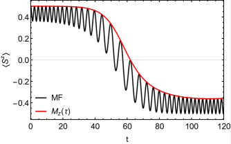
Figure 3: Numerical solution of the mean field equations (black) and the solution for the slow component $M_{z}\left(\tau\right)$ (red) using the flow equation. Parameters:$B_{z}=\Delta_{z}=0$, $\Delta_{\perp}/B_{\perp}=0.03$, $A/B_{\perp}=0.05$ and $N=100$, with central spin initially up and a fully polarized bath. The slow component perfectly describes the instanton transition.

This shows that dRG can be used to separate the dynamics according to their time scales, and study each of them independently. Furthermore, the flow equations for the central spin (Eq.30), demonstrate that the instanton transition is exponentially fast, with exponent proportional to $\Delta_{\perp}$.

IV.3 Correlation effects

The mean field equations neglect correlations between the central spin and the bath spins. That is why they fail to capture the suppression of coherent oscillations in Fig.2. To show this, we go one step further and calculate the equation of motion for the bath-system correlators:

$$\partial_{t}I_{i}^{\beta}S^{\alpha} = \left[\epsilon_{x\alpha\theta}B_{\perp}+\epsilon_{z\alpha\theta}\left(B_{z}-\sum_{j\neq i}A_{j}I_{j}^{z}\right)\right]I_{i}^{\beta}S^{\theta}$$ (33)

$$+\left(\epsilon_{x\beta\theta}\Delta_{\perp}+\epsilon_{z\beta\theta}\Delta_{z}\right)I_{i}^{\theta}S^{\alpha}$$

$$-\frac{A_{i}}{4}\left(\delta_{z,\beta}\epsilon_{z\alpha\theta}S^{\theta}+\delta_{\alpha,z}\epsilon_{z\beta\theta}I_{i}^{\theta}\right)$$

As expected, this equation couples to three-point correlators and requires a decoupling scheme to find a solution. We have considered three different decoupling schemes, which are discussed in the Appendix. The one based on a Hierarchy of Correlations is the one that gives the best results, at least for this model. This decoupling scheme has been previously discussed(Hierarchy, ), and it is based on the decomposition $\langle I_{i}^{\beta}S^{\alpha}\rangle=\langle I_{i}^{\beta}\rangle\langle S^{\alpha}\rangle+\langle I_{i}^{\beta}S^{\alpha}\rangle^{c}$, where $\langle\ldots\rangle^{c}$ indicates the correlated part, which is defined as the difference between the mean field and the exact value. The reason why this decomposition works better than the other ones considered is because it organizes the non-linear corrections in a way that they tend to be always small, compared with the mean field value.

The separation into correlated and uncorrelated parts leads to the next final equation of motion for the correlated parts:

$$\partial_{t}\langle I_{i}^{\beta}S^{\alpha}\rangle^{c} \simeq \epsilon_{z\alpha\mu}\left(B_{z}-\sum_{j\neq i}^{N}A_{j}\langle I_{j}^{z}\rangle\right)\langle I_{i}^{\beta}S^{\mu}\rangle^{c}$$ (34)

$$+\epsilon_{x\alpha\mu}B_{\perp}\langle I_{i}^{\beta}S^{\mu}\rangle^{c}$$

$$-\epsilon_{z\alpha\mu}A_{i}\langle S^{\mu}\rangle\left(\frac{\delta_{z,\beta}}{4}-\langle I_{i}^{\beta}\rangle\langle I_{i}^{z}\rangle\right)$$

$$-\epsilon_{z\beta\nu}A_{i}\langle I_{i}^{\nu}\rangle\left(\frac{\delta_{z,\alpha}}{4}-\langle S^{\alpha}\rangle\langle S^{z}\rangle\right)$$

In order to obtain Eq.34 we have assumed that correlated parts are small (at least for short time), neglected bath-bath correlators and terms proportional to $\vec{\Delta}$. These terms can be neglected because they produce slower dynamics, however, finding the solution in their presence is not difficult (detailed derivation in the Appendix). This equation must be numerically solved simultaneously with the equations for the bath and central spin:

$$\partial_{t}\langle S^{\alpha}\rangle \simeq \sum_{\mu,\theta}\epsilon_{\mu\alpha\theta}\left(B_{\mu}-\sum_{i=1}^{N}A_{i}^{\mu}\langle I_{i}^{\mu}\rangle\right)\langle S^{\theta}\rangle$$

$$-\sum_{\mu,\theta}\epsilon_{\mu\alpha\theta}\sum_{i=1}^{N}A_{i}^{\mu}\langle I_{i}^{\mu}S^{\theta}\rangle^{c}$$

$$\partial_{t}\langle I_{i}^{\alpha}\rangle \simeq \sum_{\mu,\theta}\epsilon_{\mu\alpha\theta}\left(\Delta_{\mu}-A_{i}^{\mu}\langle S^{\mu}\rangle\right)\langle I_{i}^{\theta}\rangle$$ (36)

where we have also neglected the slow terms in the equation of motion for the bath spin, which are proportional to the correlated part. The numerical solution of the equations of motion, including spin-bath correlators is shown in Fig.4. It shows that the addition of lowest order corrections, due to system-bath correlations, allows to capture the suppression of coherent oscillations. At longer time-scales other processes involving many-body correlations take over, but the qualitative behavior of the magnetization is correctly captured. This can be fixed by including extra terms in the equation of motion for the system-bath correlations.

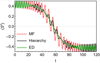
Figure 4: Comparison between the mean field solution (red), the solution including spin-bath correlations (black) and the exact simulation (green) for the same parameters as Fig.2.

As we know that Eq.34 correctly captures the main features of the dynamics, we now analyze the equations using dRG, to unravel the role of correlations between spins. Importantly, this time it will lead to flow equations for the quantum correlations between the spins, and demonstrate which contributions are crucial as time evolves, even for initial product states where correlations vanish.

For the perturbative solution we expand again, in powers of $\epsilon$, the equations of motion (Eqs.34, IV.3 and 36). For simplicity, we also assume that correlated parts are small and attach a factor $\epsilon$ to them in Eqs.IV.3 and 36. This will indeed be the case at short time, if the system initially is uncorrelated with the bath. However, it neglects an important backreaction between fluctuations and mean field values that will affect the frequency of the oscillations. Because correlated parts are proportional to $\epsilon$, to lowest order the equations of motion still are the mean field equations previously solved, with the addition of the lowest order equation of motion for the correlated part:

$$\partial_{t}\langle I_{i}^{\beta}S^{\alpha}\rangle_{0}^{c} \simeq \left(\epsilon_{z\alpha\mu}\omega_{z}+\epsilon_{x\alpha\mu}B_{\perp}\right)\langle I_{i}^{\beta}S^{\mu}\rangle_{0}^{c}$$ (37)

This equation is analogous to the one for the central spin (Eq.20), with just different boundary condition. To first order in $\epsilon$ the bath equation of motion is still unchanged with respect to the mean field case, as correlation terms are of order $\epsilon^{2}$. This is not the case for the central spin, where correlated and uncorrelated parts couple in the equation of motion:

$$\partial_{t}\langle S^{\alpha}\rangle_{1} = \sum_{\mu,\theta}\epsilon_{\mu\alpha\theta}\left(B_{\mu}-\sum_{i=1}^{N}A_{i}^{\mu}m_{i}^{\mu}\right)\langle S^{\theta}\rangle_{1}$$

$$-\sum_{\mu,\theta}\epsilon_{\mu\alpha\theta}\langle S^{\theta}\rangle_{0}\sum_{i=1}^{N}A_{i}^{\mu}\langle I_{i}^{\mu}\rangle_{1}$$

$$-\epsilon\sum_{\mu,\theta}\epsilon_{\mu\alpha\theta}\sum_{i=1}^{N}A_{i}^{\mu}\langle I_{i}^{\mu}S^{\theta}\rangle_{0}^{c}$$

where the last line corresponds to the lowest order solution for the correlated part. The solution displays once again secular terms, however, the addition of correlations produces corrections to the flow equations obtained in the mean field case (Eq.30). They are now given by:

$$\partial_{\tau}\log\left(B_{\perp}M_{x}+M_{z}\omega_{z}\right) = \epsilon\Delta_{\perp}\omega_{z}\frac{\eta_{y}}{\Omega_{\vec{m}}^{2}}$$ (39)

$$\partial_{\tau}\left(B_{\perp}M_{z}-\omega_{z}M_{x}\right) = \epsilon\omega_{z}\Delta_{\perp}\eta_{y}\frac{B_{\perp}M_{z}-\omega_{z}M_{x}}{\Omega_{\vec{m}}^{2}}$$

$$+\epsilon\omega_{z}a_{zy}$$

$$\partial_{\tau}M_{y} = \epsilon\omega_{z}\frac{a_{zx}\omega_{z}-B_{\perp}a_{zz}}{\Omega_{\vec{m}}^{2}}$$

where $a_{\alpha\beta}=\sum_{i}A_{i}c_{i}^{\alpha\beta}$, and $c_{i}^{\alpha\beta}\left(t_{0}\right)$ is the initial condition for the correlated part $\langle I_{i}^{\alpha}S^{\beta}\rangle^{c}$. The most important change with respect to the mean field case (Eq.30) is that now $M_{y}$ can flow, and that the boundary condition for the correlated part also affects the longitudinal and transverse magnetization. Furthermore, assuming that correlations do not develop over time ($a_{\alpha\beta}\left(\tau\right)=0\ \forall\ \tau$), one recovers the mean field flow equations.

As previously mentioned, the addition of correlated parts implies that now their boundary conditions $c_{i}^{\alpha\beta}$ will be renormalized over time, if the solution to the equation of motion to first order in $\epsilon$ has secular terms:

$$\partial_{t}\langle I_{i}^{\beta}S^{\alpha}\rangle_{1}^{c} \simeq \left(\epsilon_{z\alpha\mu}\omega_{z}+\epsilon_{x\alpha\mu}B_{\perp}\right)\langle I_{i}^{\beta}S^{\mu}\rangle_{1}^{c}$$

$$-\epsilon_{z\alpha\mu}\langle I_{i}^{\beta}S^{\mu}\rangle_{0}^{c}\sum_{j\neq i}^{N}A_{j}\langle I_{j}^{z}\rangle_{1}$$

$$-\epsilon_{z\alpha\mu}\epsilon A_{i}\langle S^{\mu}\rangle_{0}\left(\frac{\delta_{z,\beta}}{4}-m_{i}^{\beta}m_{i}^{z}\right)$$

$$-\epsilon_{z\beta\nu}\epsilon A_{i}m_{i}^{\nu}\left(\frac{\delta_{z,\alpha}}{4}-\langle S^{\alpha}\rangle_{0}\langle S^{z}\rangle_{0}\right)$$

This is the case, and the flow equations for the initial correlations are given by:

$$\partial_{\tau}\log\left(B_{\perp}a_{zx}+a_{zz}\omega_{z}\right) = \epsilon\Delta_{\perp}\omega_{z}\frac{\eta_{y}}{\Omega_{\vec{m}}^{2}}$$ (41)

$$\partial_{\tau}\left(B_{\perp}a_{zz}-a_{zx}\omega_{z}\right) = \epsilon\Delta_{\perp}\omega_{z}\frac{\eta_{y}}{\Omega_{\vec{m}}^{2}}\left(B_{\perp}a_{zz}-a_{zx}\omega_{z}\right)$$ (42)

$$+\epsilon M_{y}\omega_{z}\xi_{z}$$

$$\partial_{\tau}a_{zy} = -\epsilon\frac{\xi_{z}\omega_{z}}{\Omega^{2}}\left(B_{\perp}M_{z}-\omega_{z}M_{x}\right)$$ (43)

where we have defined $\xi_{z}=\sum_{i=1}^{N}A_{i}^{2}\left(\frac{1}{4}-\left(m_{i}^{z}\right)^{2}\right)$. The suppression of oscillations is obtained due to the $\xi_{z}$ function, which captures the precession of the bath magnetization away from the longitudinal axis. Also, even for vanishing initial correlations, $a_{zy}\left(\tau\right)$ becomes non-negligible over time, as it is proportional to $\xi_{z}$ and to the central spin magnetization. Fig.5 shows a comparison between the exact dynamics, the one numerically obtained by the hierarchy of correlations decoupling and its lowest order approximation obtained from dRG.

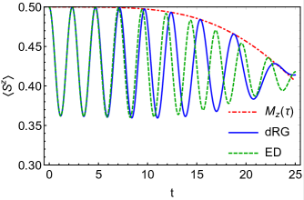
Figure 5: Comparison between the exact dynamics (dashed, green) and the lowest order solution using dRG (blue) for the same parameters as Fig.2. The red dot-dashed line shows $M_{z}\left(\tau\right)$, which plays the role of the envelope function for the faster oscillations. The lowest order solution correctly captures the suppression of oscillations, but the frequency is shifted because backreaction between the mean field solution and the correlations has been neglected at this order of dRG.

It can be seen that the first order approximation provides good agreement for the amplitude renormalization, however there is a frequency shift with respect to the exact solution. The reason for this discrepancy is that the backreaction between uncorrelated and correlated parts was neglected to lowest order, which only holds for short times (In Fig.4 this is included and one can see that the frequency of the exact solution and that of the numerical solution of Eq.34 coincide).

V Conclusions

We have shown that it is possible to obtain good approximations for the dynamics of strongly correlated systems, such as the central spin model, by numerical and analytical methods.

In the first part we have discussed the differences between an external magnetic field and a static spin bath by calculating the exact solution of the model. Then, we have demonstrated that when the environment is in an excited state, destructive interference between different quantum states results in a suppression of the coherent oscillations, which can be characterized by a Gaussian spectral function. This is not a decoherence process however, as entanglement between the two systems is not created, and it can be reversed with spin echo. Importantly, it is interesting that the suppression is highly dependent on the Zeeman splitting of the central spin. This property can be used to characterize some of the properties of the environment.

In the second part we have included a transverse field acting on the bath spins, to switch-on their dynamics. It is shown that non-perturbative effects can be important after a short time. We have numerically solved the model finding that, a separation of the equations of motion into mean field and quantum fluctuations, provides good agreement with the exact dynamics, once the lowest order fluctuations are added. The main features of this model are: Amplitude modulation, and the suppression of coherent oscillations due to entanglement with the environment. On the one hand, the amplitude modulation, which produces an instanton-like transition, is well captured at the mean field level. On the other hand, the suppression of coherent oscillations requires the quantum fluctuations to be included. Importantly, the suppression of oscillations in the case of a dynamical bath is linked with the formation of entanglement with the spin bath, unlike in the case of a static bath, and cannot generally be removed by spin echo techniques (the spin bath is precessing under a different magnetic field $\vec{\Delta}$).

Finally, we have shown that the equations of motion for the model can be analyzed using dynamical Renormalization Group techniques. The advantages of this technique are several: i) It provides an analytical approach to the highly complex numerical solutions, ii) Provides non-perturbative results, and iii) it can eliminate secular terms, even when they are present in the full numerical solution. It is also interesting that when quantum fluctuations are included, one finds non-perturbative expressions for the entanglement between system and environment, which can be useful for state preparation in experiments with many particles.

Our results can be easily applied to study the dynamics of other models of qubits interacting with surrounding localized modes, which is important for the design of quantum computers, as these are expected to dominate $T_{2}$ at low temperatures(KaneQC, ; StampNature, ; TheoryBathSpin2000, ; AdjustableSpinBath, ). Furthermore, we expect this approach to be able to characterize the decoherence rates in cases where simple Markovian solutions can fail.

Appendix A Exact solution for a static bath

The dynamics for a central spin, longitudinally coupled to a static bath of spins can be exactly solved. Starting from the Hamiltonian in Eq.1, one can make use of the basis of eigenstates for the case with $B_{\perp}=\Delta_{\perp}=0$, given by $|S,M;\vec{P},\vec{m}\rangle$, where $S$ indicates the spin value of the central spin, $M\in\left[-S,S\right]$ its projection onto the z-axis, $\vec{P}=\left(P_{1},P_{2},\ldots,P_{N}\right)$ is the spin value of the different bath spins, and $\vec{m}=\left(m_{1},m_{2},\ldots,m_{N}\right)$ their projection $m_{i}\in\left[-P_{i},P_{i}\right]$. The Hamiltonian in this basis is given by:

$$H_{0} = \sum_{S,\vec{P}}\sum_{M,\vec{m}}\left(-B_{z}M-\Delta_{z}\sum_{i}m_{i}+M\sum_{i}A_{i}m_{i}\right)X_{\vec{m},\vec{m}}^{M,M}$$ (44)

$$V_{S} = -\frac{B_{\perp}}{2}\left(S^{+}+S^{-}\right)=-\frac{B_{\perp}}{2}\sum_{S,\vec{P}}\sum_{M,\vec{m}}\gamma_{S,M}\left(X_{\vec{m},\vec{m}}^{M+1,M}+X_{\vec{m},\vec{m}}^{M,M+1}\right)$$ (45)

$$V_{B} = -\frac{\Delta_{\perp}}{2}\sum_{i}\left(I_{i}^{+}+I_{i}^{-}\right)=-\frac{\Delta_{\perp}}{2}\sum_{i}\sum_{S,\vec{P}}\sum_{M,\vec{m}}\gamma_{P_{i},m_{i}}\left(X_{\vec{m}+1_{i},\vec{m}}^{M,M}+X_{\vec{m},\vec{m}+1_{i}}^{M,M}\right)$$ (46)

where $X_{\vec{m},\vec{m}^{\prime}}^{M,M^{\prime}}=|S,M;\vec{P},\vec{m}\rangle\langle S^{\prime},M^{\prime};\vec{P}^{\prime},\vec{m}^{\prime}|$ are the Hubbard operators, $\gamma_{P_{i},m_{i}}=\sqrt{P_{i}\left(P_{i}+1\right)-m_{i}\left(m_{i}+1\right)}$ and $\vec{m}\pm 1_{i}$ indicates that for the spin configuration $\vec{m}$, the spin projection $m_{i}\rightarrow m_{i}\pm 1$, leaving all the other $m_{j}$, for all $j\neq i$, unchanged.

For the present case with $S=1/2$, we can easily diagonalize $H_{0}+V_{S}$, because the Hilbert space factorizes in different bath configurations $\vec{m}$. The equations of motion for the different projection operators $X_{\vec{m},\vec{m}}^{\pm,\pm}$ are obtained in the Heisenberg picture using the Heisenberg equation of motion $\partial_{t}\hat{O}=i\left[H,\hat{O}\right]$:

$$\partial_{t}X_{\vec{m},\vec{m}^{\prime}}^{+,+} = i\left(\omega_{\vec{m}}^{+}-\omega_{\vec{m}^{\prime}}^{+}\right)X_{\vec{m},\vec{m}^{\prime}}^{+,+}-i\frac{B_{\perp}}{2}\left(X_{\vec{m},\vec{m}^{\prime}}^{-,+}-X_{\vec{m},\vec{m}^{\prime}}^{+,-}\right)$$ (47)

$$\partial_{t}X_{\vec{m},\vec{m}^{\prime}}^{-,-} = i\left(\omega_{\vec{m}}^{-}-\omega_{\vec{m}^{\prime}}^{-}\right)X_{\vec{m},\vec{m}^{\prime}}^{-,-}-i\frac{B_{\perp}}{2}\left(X_{\vec{m},\vec{m}^{\prime}}^{+,-}-X_{\vec{m},\vec{m}^{\prime}}^{-,+}\right)$$ (48)

$$\partial_{t}X_{\vec{m},\vec{m}^{\prime}}^{+,-} = i\left(\omega_{\vec{m}}^{+}-\omega_{\vec{m}^{\prime}}^{-}\right)X_{\vec{m},\vec{m}^{\prime}}^{+,-}-i\frac{B_{\perp}}{2}\left(X_{\vec{m},\vec{m}^{\prime}}^{-,-}-X_{\vec{m},\vec{m}^{\prime}}^{+,+}\right)$$ (49)

$$\partial_{t}X_{\vec{m},\vec{m}^{\prime}}^{-,+} = i\left(\omega_{\vec{m}}^{-}-\omega_{\vec{m}^{\prime}}^{+}\right)X_{\vec{m},\vec{m}^{\prime}}^{-,+}-i\frac{B_{\perp}}{2}\left(X_{\vec{m},\vec{m}^{\prime}}^{+,+}-X_{\vec{m},\vec{m}^{\prime}}^{-,-}\right)$$ (50)

with $\omega_{\vec{m}}^{M}=-M\left(B_{z}-\vec{A}\cdot\vec{m}\right)-\Delta_{z}\sum_{i}m_{i}$. The solutions can be directly obtained; however as we are interested in the central spin dynamics, the solution for the time evolution of the different central spin operators is even simpler (because they are diagonal in the bath indices):

$$S_{\vec{m}}^{x}\left(t\right) = S_{\vec{m}}^{x}\frac{B_{\perp}^{2}+\left(B_{z}-\vec{A}\cdot\vec{m}\right)^{2}\cos\left(\Omega_{\vec{m}}t\right)}{\Omega_{\vec{m}}^{2}}+S_{\vec{m}}^{y}\frac{B_{z}-\vec{A}\cdot\vec{m}}{\Omega_{\vec{m}}}\sin\left(\Omega_{\vec{m}}t\right)+S_{\vec{m}}^{z}\frac{B_{\perp}\left(B_{z}-\vec{A}\cdot\vec{m}\right)}{\Omega_{\vec{m}}^{2}}\left[1-\cos\left(\Omega_{\vec{m}}t\right)\right]$$ (51)

$$S_{\vec{m}}^{y}\left(t\right) = S_{\vec{m}}^{y}\cos\left(\Omega_{\vec{m}}t\right)+\frac{S_{\vec{m}}^{z}B_{\perp}-S_{\vec{m}}^{x}\left(B_{z}-\vec{A}\cdot\vec{m}\right)}{\Omega_{\vec{m}}}\sin\left(\Omega_{\vec{m}}t\right)$$ (52)

$$S_{\vec{m}}^{z}\left(t\right) = S_{\vec{m}}^{z}\frac{\left(B_{z}-\vec{A}\cdot\vec{m}\right)^{2}+B_{\perp}^{2}\cos\left(\Omega_{\vec{m}}t\right)}{\Omega_{\vec{m}}^{2}}-S_{\vec{m}}^{y}B_{\perp}\frac{\sin\left(\Omega_{\vec{m}}t\right)}{\Omega_{\vec{m}}}+S_{\vec{m}}^{x}B_{\perp}\left(B_{z}-\vec{A}\cdot\vec{m}\right)\frac{1-\cos\left(\Omega_{\vec{m}}t\right)}{\Omega_{\vec{m}}^{2}}$$ (53)

where we have just rewritten the equations of motion in the basis of spin operators for a given bath configuration:

$$S_{\vec{m}}^{x}\left(t\right) = \frac{1}{2}\left(X_{\vec{m},\vec{m}}^{+,-}\left(t\right)+X_{\vec{m},\vec{m}}^{-,+}\left(t\right)\right)$$

$$S_{\vec{m}}^{y}\left(t\right) = -\frac{i}{2}\left(X_{\vec{m},\vec{m}}^{+,-}\left(t\right)-X_{\vec{m},\vec{m}}^{-,+}\left(t\right)\right)$$

$$S_{\vec{m}}^{z}\left(t\right) = \frac{1}{2}\left(X_{\vec{m},\vec{m}}^{+,+}\left(t\right)-X_{\vec{m},\vec{m}}^{-,-}\left(t\right)\right)$$

In the previous expressions we have defined the frequency for a given bath configuration $\Omega_{\vec{m}}=\sqrt{B_{\perp}^{2}+\left(B_{z}-\vec{A}\cdot\vec{m}\right)^{2}}$. The total time evolution for the magnetization is given by $\vec{S}\left(t\right)=\sum_{\vec{P},\vec{m}}\vec{S}_{\vec{m}}\left(t\right)$, which requires to sum over all spin bath configurations. In the next Appendix it is shown how one can easily do this.

Appendix B Sum over polarization groups

The exact expression for the magnetization of the central spin requires to sum over all spin bath configurations, and depending on the initial state, the results can be quite different. First of all, it is useful to consider a situation where the initial state for the total system is a product state, as typically an experiment can control the central spin/qubit, but not the environmental degrees of freedom:

$$\rho\left(t_{0}\right) = \rho_{S}\otimes\rho_{B}$$ (54)

This is only useful for our discussion, but not required for the derivation. Now it is important to realize that two opposite situations can happen: The environment it is either in its ground state (i.e., the temperature is low enough that just the lowest energy states are occupied), or its in a high temperature state (i.e., thermal activation equally occupies all the bath modes). In the first case, the sum over bath configurations is dominated by a single term and the sum does not need to be calculated. This implies that the central spin dynamics will only contain a single frequency and the dynamics can be easily understood. In the second case the sum has a huge number of frequencies, and the total summation can be cumbersome. In this case, some approximate method to simplify the sum would be desirable. In this case it is useful to consider a density of states (DOS) $J\left(\alpha\right)$ such that:

$$\vec{S}\left(t\right) = \sum_{\vec{P},\vec{m}}\vec{S}_{\vec{m}}\left(t\right)=\int_{-\infty}^{\infty}d\alpha\vec{S}\left(t,\alpha\right)J\left(\alpha\right)$$ (55)

$$J\left(\alpha\right) \equiv \sum_{\vec{m}}g_{\vec{m}}\delta\left(\alpha-B_{z}+\vec{A}\cdot\vec{m}\right)$$ (56)

where $g_{\vec{m}}$ accounts for the degeneracy of each polarization group configuration. Using a Fourier transform one can rewrite the DOS as:

$$J\left(\alpha\right) = \int_{-\infty}^{\infty}\frac{d\epsilon}{2\pi}\sum_{\vec{m}}g_{\vec{m}}e^{i\epsilon\left(\alpha-B_{z}+\vec{A}\cdot\vec{m}\right)}$$

$$= \int_{-\infty}^{\infty}\frac{d\epsilon}{2\pi}e^{i\epsilon\left(\alpha-B_{z}\right)}\prod_{i=1}^{N}\sum_{m_{i}=-P_{i}}^{P_{i}}g_{m_{i}}e^{i\epsilon A_{i}m_{i}}$$

where $g_{m_{i}}=P_{i}-\left|m_{i}\right|+1$. At this point, depending on the spin value $P_{i}$, one can approximate the sum as an integral if $P_{i}\gg 1/2$. If this is not the case one can directly calculate the sum, but we will consider the case $P_{i}\gg 1$, because it leads to more compact expressions and is valid in many cases. Finally, one can calculate the large product $\prod_{i=1}^{N}$ using a stationary phase approximation, which leads to the final expression for the normalized DOS:

$$J\left(\alpha\right)=\frac{e^{-\frac{\left(\alpha-B_{z}\right)^{2}}{2\sigma^{2}}}}{\sqrt{2\pi\sigma^{2}}},\ \sigma\equiv\sqrt{\frac{1}{6}\sum_{i}A_{i}^{2}P_{i}^{2}\frac{P_{i}+4}{P_{i}+2}}$$ (58)

This indicates that for the case of broadening larger than the hyperfine splitting, the effect of the bath is similar to an statistical average over a bias field with Gaussian fluctuations. Furthermore, the Gaussian broadens as $N^{1/2}$ with the number of bath spins $N$, and also linearly with $A_{i}$ and $P_{i}$. This implies that the final expression for the central spin magnetization, is given by:

$$\vec{S}\left(t\right)=\int_{-\infty}^{+\infty}\vec{S}_{\alpha}\left(t\right)J\left(\alpha\right)d\alpha$$ (59)

with $\Omega_{\alpha}=\sqrt{B_{\perp}^{2}+\alpha^{2}}$. The expressions for the time evolution of the different components of the central spin magnetization become:

$$S_{\alpha}^{x}\left(t\right) = S^{x}\frac{B_{x}^{2}+\alpha^{2}\cos\left(\Omega_{\alpha}t\right)}{\Omega_{\alpha}^{2}}+S^{y}\frac{\alpha}{\Omega_{\alpha}}\sin\left(\Omega_{\alpha}t\right)+S^{z}\frac{B_{\perp}\alpha}{\Omega_{\alpha}^{2}}\left[1-\cos\left(\Omega_{\alpha}t\right)\right]$$ (60)

$$S_{\alpha}^{y}\left(t\right) = S^{y}\cos\left(\Omega_{\alpha}t\right)+\frac{S^{z}B_{x}-S^{x}\alpha}{\Omega_{\alpha}}\sin\left(\Omega_{\alpha}t\right)$$ (61)

$$S_{\alpha}^{z}\left(t\right) = S^{z}\frac{\alpha^{2}+B_{\perp}^{2}\cos\left(\Omega_{\alpha}t\right)}{\Omega_{\alpha}^{2}}-B_{\perp}S^{y}\frac{\sin\left(\Omega_{\alpha}t\right)}{\Omega_{\alpha}}+B_{\perp}\alpha S^{x}\frac{1-\cos\left(\Omega_{\alpha}t\right)}{\Omega_{\alpha}^{2}}$$ (62)

For intermediate temperature regimes, one can consider a thermal distribution for the occupation of the different hyperfine levels, but at high enough $T$, its value is equal for all of them. These expressions are valid up to some long recurrence time $\tau_{P}\sim A_{i}^{-1}$ for $A_{i}$ small, but the integral with the Gaussian function produces a behavior that emulates decoherence, as it is shown in Fig.1. Furthermore, the recurrence time will not be typically captured in experiments, because at long times, one expects that phonons and other delocalized modes will take over. Hence this result should be a very good approximation to describe the short time dynamics under the influence of an almost static spin bath.

Interestingly, when the standard deviation $\sigma$ is of the order of the central spin splitting $\sigma/B_{z}\sim 1$, coherent oscillations are only weakly damped, indicating that this could be a good regime to operate with the qubit. It also would allow to experimentally access to information about the bath, by sweeping over $B_{z}$ and monitoring the dynamics (to estimate the number of modes, their spin or the coupling strength). Finally, the assumption of high temperature in the bath is not strictly necessary, and this result is valid for any case where the bath state is a large superposition of different configurations, even at $T=0$. Notice that the resulting suppression of the coherent oscillations is not due to a disorder bias average (it also happens for the case $A_{i}=A$), but it is a consequence of the bath being a quantum system which can be in a superposition state, and the different phases of the different configurations interfere destructively. This indicates that the spin bath cannot be simply thought as a classical magnetic field.

Appendix C Perturbative dynamics

When the transverse field acting on the bath is turned on, different spin configurations couple, and for large systems, the exact calculation becomes cumbersome. To estimate the effect of the transverse field acting on the bath spins, it is useful to transform to the basis of eigenstates for $H_{S}=H_{0}+V_{S}$. As the Hamiltonian is diagonal in the bath configurations $\vec{m}$, the diagonalization is simple and leads to:

$$H_{S} = \sum_{\vec{P},\vec{m}}H_{S}\left(\vec{m}\right)$$ (63)

$$H_{S}\left(\vec{m}\right) = \left(\begin{array}[]{cc}-\Delta_{z}\sum_{i}m_{i}-\frac{B_{z}}{2}+\frac{\vec{A}}{2}\cdot\vec{m}&-\frac{B_{\perp}}{2}\\ -\frac{B_{\perp}}{2}&-\Delta_{z}\sum_{i}m_{i}+\frac{B_{z}}{2}-\frac{\vec{A}}{2}\cdot\vec{m}\end{array}\right)$$ (66)

with eigenvalues

$$E_{\vec{m}}^{M}=-\Delta_{z}\sum_{i}m_{i}+M\sqrt{B_{\perp}^{2}+\left(B_{z}-\vec{A}\cdot\vec{m}\right)^{2}}$$ (67)

In this basis the full Hamiltonian becomes:

$$H = \sum_{\vec{P},\vec{m},M}\left[E_{\vec{m}}^{M}X_{\vec{m},\vec{m}}^{M,M}-\frac{\Delta_{\perp}}{2}\sum_{i}\gamma_{P_{i},m_{i}}\left(X_{\vec{m}+1_{i},\vec{m}}^{M,M}+X_{\vec{m},\vec{m}+1_{i}}^{M,M}\right)\right]$$ (68)

where now the index $M=\pm 1/2$ refers to the eigenstates and eigenvalues of the matrix in Eq.66. The dynamics, once the transverse bath operator is present, is obtained from the time-dependent Schrödinger equation:

$$i\partial_{t}|\Psi\left(t\right)\rangle=\left(H_{0}+V_{B}\right)|\Psi\left(t\right)\rangle$$ (69)

Using a decomposition for a general state $|\Psi\left(t\right)\rangle$ in terms of the unperturbed eigenstates $H_{0}|M,\vec{m}\rangle=E_{\vec{m}}^{M}|M,\vec{m}\rangle$, leads to (we are ignoring the indices $\vec{P}$ and $S$ because they do not play an important role. However they must be added at the end of the calculation):

$$|\Psi\left(t\right)\rangle=\sum_{M,\vec{m}}c_{M,\vec{m}}\left(t\right)e^{-itE_{\vec{m}}^{M}}|M,\vec{m}\rangle$$ (70)

We can now rewrite the time-dependent Schrödinger equation, by multiplying by $\langle M^{\prime},\vec{m}^{\prime}|$ from the left, as follows:

$$\dot{c}_{M,\vec{m}}\left(t\right)=-i\sum_{\vec{m}^{\prime}}c_{M,\vec{m}^{\prime}}\left(t\right)e^{it\left(E_{\vec{m}}^{M}-E_{\vec{m}^{\prime}}^{M}\right)}\langle\vec{m}|V_{B}|\vec{m}^{\prime}\rangle$$ (71)

where we have used that the matrix elements of $V_{B}$ only couple different bath configurations. As in this equation all the different bath configurations couple, when the bath is large, it must be truncated. For this, we consider a powers expansion:

$$c_{M,\vec{m}}\left(t\right)=c_{M,\vec{m}}^{\left(0\right)}+\Delta_{\perp}c_{M,\vec{m}}^{\left(1\right)}\left(t\right)+\Delta_{\perp}^{2}c_{M,\vec{m}}^{\left(2\right)}\left(t\right)+\ldots$$ (72)

Similarly, the calculation of the matrix elements yields:

$$\langle M,\vec{m}|V_{B}|M^{\prime},\vec{m}^{\prime}\rangle = -\frac{\Delta_{\perp}}{2}\sum_{i=1}^{N}\left(\gamma_{P_{i},m_{i}^{\prime}}\delta_{\vec{m}^{\prime}+1_{i},\vec{m}}+\gamma_{P_{i},m_{i}}\delta_{\vec{m}+1_{i},\vec{m}^{\prime}}\right)$$ (73)

Then inserting this result in the calculation of the $c_{M,\vec{m}}^{\left(n+1\right)}\left(t\right)$ we get the next expression for the different orders of the expansion:

$$\dot{c}_{M,\vec{m}}^{\left(n+1\right)}\left(t\right) = \frac{i}{2}\sum_{i=1}^{N}\gamma_{P_{i},m_{i}-1}c_{M,\vec{m}-1_{i}}^{\left(n\right)}\left(t\right)e^{-it\left(E_{\vec{m}-1_{i}}^{M}-E_{\vec{m}}^{M}\right)}$$ (74)

$$+\frac{i}{2}\sum_{i=1}^{N}\gamma_{P_{i},m_{i}}c_{M,\vec{m}+1_{i}}^{\left(n\right)}\left(t\right)e^{-it\left(E_{\vec{m}+1_{i}}^{M}-E_{\vec{m}}^{M}\right)}$$

To first order in $\Delta_{\perp}$, the solution adds small amplitude corrections of order $\Delta_{\perp}$ to the unperturbed solution, by coupling the initial state to all bath configurations where one bath spin has changed by a unit. To second order in $\Delta_{\perp}$ the solution is more involved, as it contains small amplitude corrections of order $\Delta_{\perp}^{2}$, plus a secular term:

$$i\left(t-t_{0}\right)c_{M,\vec{m}}^{\left(0\right)}\left(t_{0}\right)\left(\frac{\Delta_{\perp}}{2}\right)^{2}\sum_{i=1}^{N}\left(\frac{\gamma_{P_{i},m_{i}-1}^{2}}{E_{\vec{m}}^{M}-E_{\vec{m}-1_{i}}^{M}}+\frac{\gamma_{P_{i},m_{i}}^{2}}{E_{\vec{m}}^{M}-E_{\vec{m}+1_{i}}^{M}}\right)$$ (75)

As it is discussed in the main text, secular terms can be renormalized and give rise to non-perturbative corrections. The main idea is to assume that the boundary conditions are time-dependent, and that their series expansion produces the secular terms previously found. This leads to the next flow equation for the boundary condition:

$$\partial_{\tau}c_{M,\vec{m}}^{\left(0\right)}\left(\tau\right)\simeq ic_{M,\vec{m}}^{\left(0\right)}\left(\tau\right)\left(\frac{\Delta_{\perp}}{2}\right)^{2}\sum_{i=1}^{N}\left(\frac{\gamma_{P_{i},m_{i}-1}^{2}}{E_{\vec{m}}^{M}-E_{\vec{m}-1_{i}}^{M}}+\frac{\gamma_{P_{i},m_{i}}^{2}}{E_{\vec{m}}^{M}-E_{\vec{m}+1_{i}}^{M}}\right)$$ (76)

with solution

$$c_{M,\vec{m}}^{\left(0\right)}\left(t\right)=c_{M,\vec{m}}^{\left(0\right)}\left(t_{0}\right)\prod_{i=1}^{N}e^{i\left(t-t_{0}\right)\left(\frac{\Delta_{\perp}}{2}\right)^{2}\left(\frac{\gamma_{P_{i},m_{i}-1}^{2}}{E_{\vec{m}-1_{i}}^{M}-E_{\vec{m}}^{M}}+\frac{\gamma_{P_{i},m_{i}}^{2}}{E_{\vec{m}+1_{i}}^{M}-E_{\vec{m}}^{M}}\right)}$$ (77)

This solution implies that the renormalized solution will oscillate with a shifted frequency due to the dynamical bath, but it does not affect the amplitude. Importantly, one must notice that the shift in frequency could not be obtained perturbatively; however, the instanton transition is not captured.

Appendix D Dynamical RG analysis of Mean Field equations

The general equations of motion for the system are given by:

$$\partial_{t}S^{\alpha} = \sum_{\mu}\epsilon_{\mu\alpha\theta}\left(B_{\mu}-\sum_{i=1}^{N}A_{i}^{\mu}I_{i}^{\mu}\right)S^{\theta}$$ (78)

$$\partial_{t}I_{i}^{\alpha} = \sum_{\mu}\epsilon_{\mu\alpha\theta}\left(\Delta_{\mu}-S^{\mu}A_{i}^{\mu}\right)I_{i}^{\theta}$$ (79)

Making use of the mean field decoupling for the statistical averages, they reduce to:

$$\partial_{t}\langle S^{\alpha}\rangle = \sum_{\mu}\epsilon_{\mu\alpha\theta}\left(B_{\mu}-\sum_{i=1}^{N}A_{i}^{\mu}\langle I_{i}^{\mu}\rangle\right)\langle S^{\theta}\rangle$$ (80)

$$\partial_{t}\langle I_{i}^{\alpha}\rangle = \epsilon\sum_{\mu}\epsilon_{\mu\alpha\theta}\left(\Delta_{\mu}-\langle S^{\mu}\rangle A_{i}^{\mu}\right)\langle I_{i}^{\theta}\rangle$$ (81)

where we have introduced the parameter $\epsilon$ to organize the different powers of perturbations (do not confuse with the Levi-Civita symbol $\epsilon_{\mu\alpha\theta}$). To lowest order in $\epsilon$, the equations of motion yield:

$$\partial_{t}\langle S^{\alpha}\rangle_{0} = \sum_{\mu}\epsilon_{\mu\alpha\theta}\left(B_{\mu}-\sum_{i=1}^{N}A_{i}^{\mu}m_{i}^{\mu}\right)\langle S^{\theta}\rangle_{0}$$ (82)

$$\partial_{t}\langle I_{i}^{\alpha}\rangle_{0} = 0\rightarrow\langle I_{i}^{\alpha}\left(t_{0}\right)\rangle_{0}=m_{i}^{\alpha}$$ (83)

where $m_{i}^{\alpha}$ are the initial conditions for the magnetization of each bath spin. The solutions are easily obtained by direct integration, and the ones for the central spin can be used to calculate the first order corrections to the bath spin dynamics:

$$\partial_{t}\langle I_{i}^{\alpha}\rangle_{1}=\epsilon\sum_{\mu}\epsilon_{\mu\alpha\theta}\left(\Delta_{\mu}-\langle S^{\mu}\rangle_{0}A_{i}^{\mu}\right)m_{i}^{\theta}$$ (84)

They solutions display fast oscillations with frequency $\Omega_{\vec{m}}=\sqrt{\sum_{\mu}\left(B_{\mu}-\sum_{i=1}^{N}A_{i}^{\mu}m_{i}^{\mu}\right)^{2}}$, and the next secular terms:

$$\langle I_{i}^{\alpha}\rangle_{1} = \ldots-t\sum_{\nu,\rho}\epsilon_{\alpha\nu\rho}m_{i}^{\nu}\left(\frac{A_{i}^{\rho}\omega_{\rho}}{\Omega_{\vec{m}}^{2}}\sum_{\mu}M_{\mu}\omega_{\mu}-\Delta_{\rho}\right)$$ (85)

where $\omega_{\mu}=B_{\mu}-\sum_{i=1}^{N}A_{i}^{\mu}m_{i}^{\mu}$ and $M_{\mu}$ is the initial condition for the central spin magnetization along the $\mu$-axis. The lowest order solution for the central spin describes a spin precessing in an effective magnetic field, combination of the external one $\vec{B}$ and the Overhauser field produced by the static bath $\sum_{i}A_{i}^{\mu}m_{i}^{\mu}$. In order to eliminate the secular terms for the bath equations of motion to first order (Eq.85), one must consider the boundary conditions time-dependent, in such a way that they become the generators of the secular terms to first order. This leads to:

$$\partial_{\tau}m_{i}^{\alpha}\left(\tau\right)=-\sum_{\nu,\rho}\epsilon_{\alpha\nu\rho}m_{i}^{\nu}\left(\tau\right)\left(\frac{A_{i}^{\rho}\omega_{\rho}\left(\tau\right)}{\Omega_{\vec{m}}\left(\tau\right)^{2}}\sum_{\mu}M_{\mu}\left(\tau\right)\omega_{\mu}\left(\tau\right)-\Delta_{\rho}\right)$$ (86)

where the $\tau$ dependence due to the boundary conditions has been explicitly added for clarity. Notice that this is a highly non-linear differential equation. As the flow equations for the boundary conditions $m_{i}^{\mu}\left(\tau\right)$ are coupled to the boundary conditions for the central spin $M_{\mu}\left(\tau\right)$, one must solve the equations of motion for the central spin to first order in $\epsilon$. The equations of motion for the central spin, to first order in $\epsilon$, are:

$$\partial_{t}\langle S^{\alpha}\rangle_{1} = \sum_{\mu}\epsilon_{\mu\alpha\theta}\omega_{\mu}\langle S^{\theta}\rangle_{1}-\sum_{\mu}\epsilon_{\mu\alpha\theta}\sum_{i=1}^{N}A_{i}^{\mu}\langle I_{i}^{\mu}\rangle_{1}\langle S^{\theta}\rangle_{0}$$ (87)

At this point it is useful to define $\eta_{\mu}=\sum_{i}A_{i}^{z}m_{i}^{\mu}=\sum_{i}A_{i}m_{i}^{\mu}$. The analytical solutions display secular terms, and for clarity, we derive in detail one of the flow equations for the central spin. For example, the solution for the $\langle S^{x}\rangle$ component is given by:

$$\langle S^{x}\left(t\right)\rangle_{1} = \epsilon B_{\perp}\Delta_{\perp}\eta_{y}\frac{B_{\perp}M_{y}\left[\cos\left(\Omega_{\vec{m}}t\right)-1\right]+M_{z}\Omega_{\vec{m}}\sin\left(\Omega_{\vec{m}}t\right)}{\Omega_{\vec{m}}^{4}}$$

$$-\epsilon tB_{\perp}\Delta_{\perp}\eta_{y}\frac{\omega_{z}\left(B_{\perp}M_{x}+M_{z}\omega_{z}\right)+B_{\perp}\left(B_{\perp}M_{z}-M_{x}\omega_{z}\right)\cos\left(\Omega_{\vec{m}}t\right)-B_{\perp}M_{y}\Omega_{\vec{m}}\sin\left(\Omega_{\vec{m}}t\right)}{\Omega_{\vec{m}}^{4}}$$

$$+\epsilon t^{2}\Delta_{\perp}\eta_{y}\omega_{z}^{2}\frac{M_{y}\Omega_{\vec{m}}\cos\left(\Omega_{\vec{m}}t\right)+\left(B_{\perp}M_{z}-M_{x}\omega_{z}\right)\sin\left(\Omega_{\vec{m}}t\right)}{2\Omega_{\vec{m}}^{3}}$$

Noticing that the unperturbed solution is given by:

$$\langle S^{x}\left(t\right)\rangle_{0}=\frac{B_{\perp}\left(B_{\perp}M_{x}+M_{z}\omega_{z}\right)-\omega_{z}\left(B_{\perp}M_{z}-M_{x}\omega_{z}\right)\cos\left(\Omega_{\vec{m}}t\right)+M_{y}\Omega_{\vec{m}}\omega_{z}\sin\left(\Omega_{\vec{m}}t\right)}{\Omega_{\vec{m}}^{2}}$$ (89)

one can derive three different flow equations: One for the cosine term, another for the sine term and a third one corresponding to the constant term. Let us derive the constant term flow equation, although the other ones are derived in exactly the same manner. Our aim is that the boundary condition for the constant term in $\langle S^{x}\left(t\right)\rangle_{0}$ encodes, to first order in $\epsilon$, the secular term obtained in $\langle S^{x}\left(t\right)\rangle_{1}$. This imposes that:

$$B_{\perp}\partial_{\tau}\frac{B_{\perp}M_{x}\left(\tau\right)+M_{z}\left(\tau\right)\omega_{z}\left(\tau\right)}{\Omega_{\vec{m}}\left(\tau\right)^{2}}=-\epsilon B_{\perp}\Delta_{\perp}\eta_{y}\left(\tau\right)\omega_{z}\left(\tau\right)\frac{B_{\perp}M_{x}\left(\tau\right)+M_{z}\left(\tau\right)\omega_{z}\left(\tau\right)}{\Omega_{\vec{m}}\left(\tau\right)^{4}}$$ (90)

Notice that the secular terms with harmonic time dependence cannot enter this flow equation, as it must be fulfilled for arbitrary time. Now one just needs to derive the l.h.s. of Eq.90 using:

$$\partial_{\tau}\frac{1}{\Omega_{\vec{m}}\left(\tau\right)^{2}} = -\frac{2\omega_{z}\left(\tau\right)}{\Omega_{\vec{m}}\left(\tau\right)^{4}}\partial_{\tau}\omega_{z}\left(\tau\right)$$ (91)

$$= -2\epsilon\Delta_{\perp}\frac{\omega_{z}\left(\tau\right)\eta_{y}\left(\tau\right)}{\Omega_{\vec{m}}\left(\tau\right)^{4}}$$

where we have applied:

$$\partial_{\tau}\omega_{z}\left(\tau\right) = -\sum_{i}A_{i}\partial_{\tau}m_{i}^{z}\left(\tau\right)$$

$$= \epsilon\Delta_{\perp}\sum_{i}A_{i}m_{i}^{y}\left(\tau\right)=\epsilon\Delta_{\perp}\eta_{y}\left(\tau\right)$$

and in the last line also Eq.86 for $\partial_{\tau}m_{i}^{z}\left(\tau\right)$. The flow equation finally becomes:

$$\partial_{\tau}\left(B_{\perp}M_{x}+M_{z}\omega_{z}\right)=\epsilon\Delta_{\perp}\omega_{z}\eta_{y}\frac{B_{\perp}M_{x}+M_{z}\omega_{z}}{\Omega_{\vec{m}}^{2}}$$ (93)

Finally, reorganizing terms one can write:

$$\partial_{\tau}\log\left(B_{\perp}M_{x}+M_{z}\omega_{z}\right)=\epsilon\Delta_{\perp}\frac{\eta_{y}\omega_{z}}{\Omega_{\vec{m}}^{2}}$$ (94)

which indicates that the running of the initial condition is triggered by the bath dynamics, as it is proportional to $\Delta_{\perp}$. The other equations are derived in a similar fashion, with the peculiarity that quadratic secular terms $\propto\epsilon t^{2}$ in Eq.D are also present for the sine and cosine terms. Their appearance is easy to understand, as they are a consequence of the time-dependent frequency $\Omega_{\vec{m}}\left(\tau\right)$. Thus, calculating their flow equation one finds:

$$\partial_{\tau}\log\left(B_{\perp}M_{z}-M_{x}\omega_{z}\right) = \epsilon\Delta_{\perp}\frac{\eta_{y}\omega_{z}}{\Omega_{\vec{m}}^{2}}$$ (95)

and

$$\partial_{\tau}M_{y} = 0$$ (96)

The numerical solution of the flow equations captures the instanton-like dynamics, with the resonant transition happening when the bath depolarizes (Fig.6). The comparison with the exact diagonalization result shows that the moment where the instanton transitions happen is well captured, however a slow decay takes over at very long time-scales. On the other hand, the suppression of coherent oscillations at short times is missed by this solution. This will be captured by adding correlations in the next section.

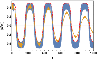
Figure 6: Comparison between the central spin dynamics between the dRG result to first order (blue) and the exact diagonalization one (yellow). The red dashed line shows the function $M_{z}\left(t\right)$, which modulates the fast coherent oscillations of the central spin. Parameters: $\Delta_{\perp}/B_{\perp}=0.03$, $A/B_{\perp}=0.05$ and $N=100$ for the initial condition $\langle S^{z}\left(0\right)\rangle=\frac{1}{2}$ and $\langle P_{z}\left(0\right)\rangle=N/2$.

Appendix E Correlations: comparison for different decoupling methods

When correlations between the system and the bath spins are included, one needs to calculate the next equation of motion:

$$\partial_{t}I_{n}^{\beta}S^{\alpha} = i\left[H,I_{n}^{\beta}S^{\alpha}\right]$$

$$= \epsilon_{z\alpha\mu}B_{z}I_{n}^{\beta}S^{\mu}+\epsilon_{x\alpha\mu}B_{\perp}I_{n}^{\beta}S^{\mu}$$

$$+\epsilon_{z\beta\nu}\Delta_{z}I_{n}^{\nu}S^{\alpha}+\epsilon_{x\beta\nu}\Delta_{\perp}I_{n}^{\nu}S^{\alpha}$$

$$-\epsilon_{z\beta\nu}A_{n}I_{n}^{\nu}S^{z}S^{\alpha}-\epsilon_{z\alpha\mu}\sum_{i=1}^{N}A_{i}I_{n}^{\beta}I_{i}^{z}S^{\mu}$$

It is important to now separate the terms $i=n$ and $i\neq n$ due their different effects. This leads to the next equation of motion:

$$\partial_{t}I_{n}^{\beta}S^{\alpha} = \left[\epsilon_{x\alpha\mu}B_{\perp}+\epsilon_{z\alpha\mu}\left(B_{z}-\sum_{i\neq n}^{N}A_{i}I_{i}^{z}\right)\right]I_{n}^{\beta}S^{\mu}$$ (98)

$$+\left(\epsilon_{z\beta\nu}\Delta_{z}+\epsilon_{x\beta\nu}\Delta_{\perp}\right)I_{n}^{\nu}S^{\alpha}$$

$$-\epsilon_{z\beta\nu}A_{n}I_{n}^{\nu}\left(\frac{\delta_{z,\alpha}}{4}+i\epsilon_{z\alpha\mu}S^{\mu}\right)-\epsilon_{z\alpha\mu}A_{n}I_{n}^{\beta}I_{n}^{z}S^{\mu}$$

Furthermore, if one considers that the bath spins are spin $1/2$, the expression simplifies to:

$$\partial_{t}I_{n}^{\beta}S^{\alpha} = \left[\epsilon_{x\alpha\mu}B_{\perp}+\epsilon_{z\alpha\mu}\left(B_{z}-\sum_{i\neq n}^{N}A_{i}I_{i}^{z}\right)\right]I_{n}^{\beta}S^{\mu}$$

$$+\left(\epsilon_{z\beta\nu}\Delta_{z}+\epsilon_{x\beta\nu}\Delta_{\perp}\right)I_{n}^{\nu}S^{\alpha}-\frac{A_{n}}{4}\left(\epsilon_{z\beta\nu}\delta_{z,\alpha}I_{n}^{\nu}+\epsilon_{z\alpha\mu}\delta_{z,\beta}S^{\mu}\right)$$

We now describe three different decoupling schemes that have been used to study their accuracy for the simulation of dynamics (Fig.7).

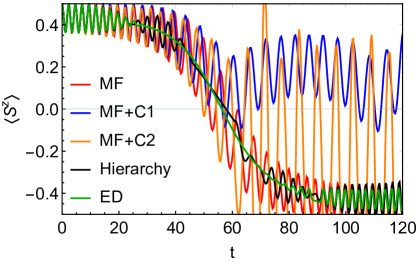
Figure 7: Comparison between different decoupling schemes

The first one consists in neglecting all correlations in Eq.E, which leads to:

$$\partial_{t}\langle I_{n}^{\beta}S^{\alpha}\rangle \simeq \left[\epsilon_{x\alpha\mu}B_{\perp}+\epsilon_{z\alpha\mu}\left(B_{z}-\sum_{i\neq n}^{N}A_{i}\langle I_{i}^{z}\rangle\right)\right]\langle I_{n}^{\beta}\rangle\langle S^{\mu}\rangle$$ (100)

$$+\left(\epsilon_{z\beta\nu}\Delta_{z}+\epsilon_{x\beta\nu}\Delta_{\perp}\right)\langle I_{n}^{\nu}\rangle\langle S^{\alpha}\rangle$$

$$-\frac{A_{n}}{4}\left(\epsilon_{z\beta\nu}\delta_{z,\alpha}\langle I_{n}^{\nu}\rangle+\epsilon_{z\alpha\mu}\delta_{z,\beta}\langle S^{\mu}\rangle\right)$$

Solving these equations, simultaneously with the ones for the central spin, results in the solutions labeled as MF+C1 in Fig.7. Unfortunately they are in disagreement with the exact result and produce an even worse approximation than the MF solution: The instanton transitions are absent, and the suppression of coherent oscillations not captured. The reason is that we have kept certain correlated parts, but eliminated others without a physical criteria, introducing unphysical non-linear terms. It is important to understand that small changes in the non-linear terms, due to how the equations are truncated, will produce small differences at short time, but in general they can be dominant at long time. This is one of the reasons why simulating dynamics can be quite complicated.

If we consider a more complex decoupling, where two-spin correlations are maintained, we can just separate the three-spin correlators as $\langle I_{i}^{z}I_{n}^{\beta}S^{\mu}\rangle\simeq\langle I_{i}^{z}\rangle\langle I_{n}^{\beta}S^{\mu}\rangle$, which mostly assumes that when fluctuations are small around $\langle I_{i}^{z}\rangle$, the solution should be accurate. The next equation is then obtained for the two-spin function:

$$\partial_{t}\langle I_{n}^{\beta}S^{\alpha}\rangle \simeq \left[\epsilon_{x\alpha\mu}B_{\perp}+\epsilon_{z\alpha\mu}\left(B_{z}-\sum_{i\neq n}^{N}A_{i}\langle I_{i}^{z}\rangle\right)\right]\langle I_{n}^{\beta}S^{\mu}\rangle$$ (101)

$$+\left(\epsilon_{z\beta\nu}\Delta_{z}+\epsilon_{x\beta\nu}\Delta_{\perp}\right)\langle I_{n}^{\nu}S^{\alpha}\rangle$$

$$-\frac{A_{n}}{4}\left(\epsilon_{z\beta\nu}\delta_{z,\alpha}\langle I_{n}^{\nu}\rangle+\epsilon_{z\alpha\mu}\delta_{z,\beta}\langle S^{\mu}\rangle\right)$$

This gives the numerical results labeled as MF+C2 in the main text. The number of coupled equations is now larger, and there is back-reaction included between the different two-point correlators. Nevertheless the numerical solution is still at large disagreement with the exact solution.

Finally, an alternative decoupling is obtained by separating the n-point functions into correlated and uncorrelated parts. Here, one must determine the equation of motion for the correlated part $\partial_{t}\langle I_{n}^{\beta}S^{\alpha}\rangle^{c}=\partial_{t}\langle I_{n}^{\beta}S^{\alpha}\rangle-\partial_{t}\langle I_{n}^{\beta}\rangle\langle S^{\alpha}\rangle$:

$$\partial_{t}\langle I_{n}^{\beta}S^{\alpha}\rangle^{c} = \epsilon_{z\alpha\mu}B_{z}\langle I_{n}^{\beta}S^{\mu}\rangle^{c}+\epsilon_{x\alpha\mu}B_{\perp}\langle I_{n}^{\beta}S^{\mu}\rangle^{c}$$

$$+\epsilon_{z\beta\nu}\Delta_{z}\langle I_{n}^{\nu}S^{\alpha}\rangle^{c}+\epsilon_{x\beta\nu}\Delta_{\perp}\langle I_{n}^{\nu}S^{\alpha}\rangle^{c}$$

$$-\epsilon_{z\alpha\mu}\sum_{i\neq n}^{N}A_{i}\left(\langle S^{\mu}\rangle\langle I_{n}^{\beta}I_{i}^{z}\rangle^{c}+\langle I_{i}^{z}\rangle\langle I_{n}^{\beta}S^{\mu}\rangle^{c}+\langle I_{n}^{\beta}I_{i}^{z}S^{\mu}\rangle^{c}\right)$$

$$-\epsilon_{z\beta\nu}A_{n}\langle I_{n}^{\nu}\rangle\left(\frac{\delta_{z,\alpha}}{4}-\langle S^{\alpha}\rangle\langle S^{z}\rangle\right)$$

$$-\epsilon_{z\alpha\mu}A_{n}\left(\frac{\delta_{z,\beta}}{4}-\langle I_{n}^{\beta}\rangle\langle I_{n}^{z}\rangle\right)\langle S^{\mu}\rangle$$

$$+A_{n}\left(\epsilon_{z\beta\nu}\langle S^{\alpha}\rangle\langle I_{n}^{\nu}S^{z}\rangle^{c}+\epsilon_{z\alpha\mu}\langle I_{n}^{\beta}\rangle\langle I_{n}^{z}S^{\mu}\rangle^{c}\right)$$

The previous equation is exact but couples to higher spin correlators. Now we assume that three-point correlation functions are subdominant, and they can be neglected (at least at short time). This results in:

$$\partial_{t}\langle I_{n}^{\beta}S^{\alpha}\rangle^{c} \simeq \epsilon_{z\alpha\mu}B_{z}\langle I_{n}^{\beta}S^{\mu}\rangle^{c}+\epsilon_{x\alpha\mu}B_{\perp}\langle I_{n}^{\beta}S^{\mu}\rangle^{c}$$

$$+\epsilon_{z\beta\nu}\Delta_{z}\langle I_{n}^{\nu}S^{\alpha}\rangle^{c}+\epsilon_{x\beta\nu}\Delta_{\perp}\langle I_{n}^{\nu}S^{\alpha}\rangle^{c}$$

$$-\epsilon_{z\alpha\mu}\sum_{i\neq n}^{N}A_{i}\left(\langle S^{\mu}\rangle\langle I_{n}^{\beta}I_{i}^{z}\rangle^{c}+\langle I_{i}^{z}\rangle\langle I_{n}^{\beta}S^{\mu}\rangle^{c}\right)$$

$$-\epsilon_{z\beta\nu}A_{n}\langle I_{n}^{\nu}\rangle\left(\frac{\delta_{z,\alpha}}{4}-\langle S^{\alpha}\rangle\langle S^{z}\rangle\right)$$

$$-\epsilon_{z\alpha\mu}A_{n}\left(\frac{\delta_{z,\beta}}{4}-\langle I_{n}^{\beta}\rangle\langle I_{n}^{z}\rangle\right)\langle S^{\mu}\rangle$$

$$+A_{n}\left(\epsilon_{z\beta\nu}\langle S^{\alpha}\rangle\langle I_{n}^{\nu}S^{z}\rangle^{c}+\epsilon_{z\alpha\mu}\langle I_{n}^{\beta}\rangle\langle I_{n}^{z}S^{\mu}\rangle^{c}\right)$$

These set of equations can be solved numerically and they give quite accurate results. However, to capture the suppression of the oscillations observed from exact diagonalization, it is enough to consider a simpler approximation of the previous equation, by neglecting the slow terms given by the bath-bath correlators $\langle I_{n}^{\beta}I_{i}^{z}\rangle^{c}\simeq 0$, the terms proportional to $\vec{\Delta}$, and the two terms in the last line. This approximation will fail at long times, but reduces the number of equations considerably. This gives the numerical results labeled as Hierarchy in the main text (Fig.4) and in Fig.7.

One important aspect introduced by the correlated parts is the appearance of quadratic terms $\langle I_{n}^{z}\rangle^{2}$ in the equation of motion, which even for large disorder, where the bath would be unpolarized on average, are non-vanishing.

It is important to notice that the correlators entering the equation of motion for the central spin magnetization are summed over all bath spins (i.e., they are proportional to $\sum_{i}A_{i}\langle I_{i}^{z}S^{\theta}\rangle^{c}$. This means that when numerically solving the equations for the correlated parts, one must solve for $\sum_{n}A_{n}\langle I_{n}^{\beta}S^{\alpha}\rangle^{c}$ and not $\langle I_{n}^{\beta}S^{\alpha}\rangle^{c}$. Therefore, the quadratic terms $\langle I_{n}^{\beta}\rangle\langle I_{n}^{z}\rangle$ require the addition of their equation of motion, as they characterize the variance of the bath, which is different to the square of its average value. However, its derivation is simple, as it can be directly linked with the previous equations of motion. For example, neglecting all correlations, they yield:

$$\partial_{t}\langle I_{n}^{\alpha}\rangle\langle I_{n}^{\beta}\rangle \simeq \Delta_{\perp}\left(\epsilon_{x\beta\theta}\langle I_{n}^{\alpha}\rangle+\epsilon_{x\alpha\theta}\langle I_{n}^{\beta}\rangle\right)\langle I_{n}^{\theta}\rangle$$

$$-A_{n}\langle S^{z}\rangle\left(\epsilon_{z\beta\theta}\langle I_{n}^{\alpha}\rangle+\epsilon_{z\alpha\theta}\langle I_{n}^{\beta}\rangle\right)\langle I_{n}^{\theta}\rangle$$

where in the last line we have factorized the system-bath operators. This is how the equations have been numerically solved in this work.

Appendix F Flow equations for the Hierarchy of correlations

To obtain the flow equations that encode the effect of amplitude renormalization using dRG we consider Eq.E with the assumption $\left|\vec{\Delta}\right|,A_{i}\ll\left|\vec{B}\right|$, as previously discussed. Then the equation has the next leading terms:

$$\partial_{t}\langle I_{n}^{\beta}S^{\alpha}\rangle^{c} \simeq \epsilon_{x\alpha\mu}B_{\perp}\langle I_{n}^{\beta}S^{\mu}\rangle^{c}+\epsilon_{z\alpha\mu}\left(B_{z}-\sum_{i\neq n}^{N}A_{i}\langle I_{i}^{z}\rangle\right)\langle I_{n}^{\beta}S^{\mu}\rangle^{c}$$

$$-\epsilon_{z\alpha\mu}A_{n}\langle S^{\mu}\rangle\left(\frac{\delta_{z,\beta}}{4}-\langle I_{n}^{\beta}\rangle\langle I_{n}^{z}\rangle\right)-\epsilon_{z\beta\nu}A_{n}\langle I_{n}^{\nu}\rangle\left(\frac{\delta_{z,\alpha}}{4}-\langle S^{\alpha}\rangle\langle S^{z}\rangle\right)$$

where we have neglected bath-bath correlators (which are proportional to $\left|\vec{\Delta}\right|$ and therefore sub-dominant) as well as the precession of the spins in their internal field $\vec{\Delta}$. The first line in Eq.F corresponds to the fastest time-scale, coming from the central spin dynamics precession, while the second line is proportional to $A_{n}$ and suppresses the amplitude of the oscillations as the spins precess away from the longitudinal axis. For the three relevant components one has:

$$\partial_{t}\langle I_{n}^{z}S^{x}\rangle^{c} = \left(B_{z}-\sum_{i\neq n}^{N}A_{i}\langle I_{i}^{z}\rangle\right)\langle I_{n}^{z}S^{y}\rangle^{c}-A_{n}\langle S^{y}\rangle\left(\frac{1}{4}-\langle I_{n}^{z}\rangle^{2}\right)$$ (106)

$$\partial_{t}\langle I_{n}^{z}S^{y}\rangle^{c} = B_{\perp}\langle I_{n}^{z}S^{z}\rangle^{c}-\left(B_{z}-\sum_{i\neq n}^{N}A_{i}\langle I_{i}^{z}\rangle\right)\langle I_{n}^{z}S^{x}\rangle^{c}+A_{n}\langle S^{x}\rangle\left(\frac{1}{4}-\langle I_{n}^{z}\rangle^{2}\right)$$ (107)

$$\partial_{t}\langle I_{n}^{z}S^{z}\rangle^{c} = -B_{\perp}\langle I_{n}^{z}S^{y}\rangle^{c}$$ (108)

Notice that if we insert the dimensionless parameter $\epsilon$, to keep track of the slow bath dynamics, the previous equations are equivalent to an expansion up to linear order in $\epsilon$. At short times the first line dominates they reduce to:

$$\partial_{t}\langle I_{n}^{z}S^{x}\rangle_{0}^{c} = \omega_{z}\langle I_{n}^{z}S^{y}\rangle_{0}^{c}$$ (109)

$$\partial_{t}\langle I_{n}^{z}S^{y}\rangle_{0}^{c} = B_{\perp}\langle I_{n}^{z}S^{z}\rangle_{0}^{c}-\omega_{z}\langle I_{n}^{z}S^{x}\rangle_{0}^{c}$$ (110)

$$\partial_{t}\langle I_{n}^{z}S^{z}\rangle_{0}^{c} = -B_{\perp}\langle I_{n}^{z}S^{y}\rangle_{0}^{c}$$ (111)

The solution is similar to the one for the central spin, but with different boundary conditions, which describe the initial correlations between system and bath. Furthermore, as one only needs its sum over all bath spins multiplied by $A_{n}$, we can solve the next equation of motion instead:

$$\partial_{t}\langle P^{z}S^{x}\rangle_{0}^{c} = \omega_{z}\langle P^{z}S^{y}\rangle_{0}^{c}$$ (112)

$$\partial_{t}\langle P^{z}S^{y}\rangle_{0}^{c} = B_{\perp}\langle P^{z}S^{z}\rangle_{0}^{c}-\omega_{z}\langle P^{z}S^{x}\rangle_{0}^{c}$$ (113)

$$\partial_{t}\langle P^{z}S^{z}\rangle_{0}^{c} = -B_{\perp}\langle P^{z}S^{y}\rangle_{0}^{c}$$ (114)

where $P^{z}=\sum_{n}A_{n}I_{n}^{z}$, and the solutions are now independent of the specific bath spin. As we assume that correlated parts are small corrections to mean field, at least for short time, and we attach to them an $\epsilon$ factor in the equations of motion for the central spin and bath spins. Therefore, the lowest order the solutions for the central spin and the bath are unchanged, as all the differences due to correlations will happen to linear order in $\epsilon$. To first order in $\epsilon$ the equations of motion for the bath spins are:

$$\partial_{t}\langle I_{i}^{x}\rangle_{1} = \epsilon\left(\Delta_{z}-A_{i}\langle S^{z}\rangle_{0}\right)m_{i}^{y}$$ (115)

$$\partial_{t}\langle I_{i}^{y}\rangle_{1} = \epsilon\Delta_{\perp}m_{i}^{z}-\epsilon\left(\Delta_{z}-A_{i}\langle S^{z}\rangle_{0}\right)m_{i}^{x}$$ (116)

$$\partial_{t}\langle I_{i}^{z}\rangle_{1} = -\epsilon\Delta_{\perp}m_{i}^{y}$$ (117)

where we have neglected the correlated terms because they are of order $\epsilon^{2}$. For the central spin, to first order in $\epsilon$, one finds:

$$\partial_{t}\langle S^{x}\rangle_{1} = \omega_{z}\langle S^{y}\rangle_{1}-\langle S^{y}\rangle_{0}\sum_{i}A_{i}\langle I_{i}^{z}\rangle_{1}-\epsilon\sum_{i}A_{i}\langle I_{i}^{z}S^{y}\rangle_{0}^{c}$$ (118)

$$\partial_{t}\langle S^{y}\rangle_{1} = B_{\perp}\langle S^{z}\rangle_{1}-\omega_{z}\langle S^{x}\rangle_{1}+\langle S^{x}\rangle_{0}\sum_{i}A_{i}\langle I_{i}^{z}\rangle_{1}+\epsilon\sum_{i}A_{i}\langle I_{i}^{z}S^{x}\rangle_{0}^{c}$$ (119)

$$\partial_{t}\langle S^{z}\rangle_{1} = -B_{\perp}\langle S^{y}\rangle_{1}$$ (120)

and for the correlations:

$$\partial_{t}\langle I_{n}^{z}S^{x}\rangle_{1}^{c} = \omega_{z}\langle I_{n}^{z}S^{y}\rangle_{1}^{c}-\langle I_{n}^{z}S^{y}\rangle_{0}^{c}\sum_{i\neq n}^{N}A_{i}\langle I_{i}^{z}\rangle_{1}-\epsilon A_{n}\langle S^{y}\rangle_{0}\left(\frac{1}{4}-\left(m_{n}^{z}\right)^{2}\right)$$ (121)

$$\partial_{t}\langle I_{n}^{z}S^{y}\rangle_{1}^{c} = B_{\perp}\langle I_{n}^{z}S^{z}\rangle_{1}^{c}-\omega_{z}\langle I_{n}^{z}S^{x}\rangle_{1}^{c}+\langle I_{n}^{z}S^{x}\rangle_{0}^{c}\sum_{i\neq n}^{N}A_{i}\langle I_{i}^{z}\rangle_{1}+\epsilon A_{n}\langle S^{x}\rangle_{0}\left(\frac{1}{4}-\left(m_{n}^{z}\right)^{2}\right)$$ (122)

$$\partial_{t}\langle I_{n}^{z}S^{z}\rangle_{1}^{c} = -B_{\perp}\langle I_{n}^{z}S^{y}\rangle_{1}^{c}$$ (123)

The appearance of new secular terms in the different solutions is what gives rise to the modified flow equations for the system. For the bath, the flow equations are identical to the mean-field case, because we have neglected the role of correlations on it:

$$\partial_{\tau}m_{i}^{x} = m_{i}^{y}\left(\Delta_{z}-A_{i}\omega_{z}\frac{B_{\perp}M_{x}+M_{z}\omega_{z}}{\Omega_{\vec{m}}^{2}}\right)$$ (124)

$$\partial_{\tau}m_{i}^{y} = m_{i}^{z}\Delta_{\perp}-m_{i}^{x}\left(\Delta_{z}-A_{i}\omega_{z}\frac{B_{\perp}M_{x}+M_{z}\omega_{z}}{\Omega_{\vec{m}}^{2}}\right)$$ (125)

$$\partial_{\tau}m_{i}^{z} = -m_{i}^{y}\Delta_{\perp}$$ (126)

The solutions for the bath to first order will now be used in the calculation for the central spin, which requires to multiply by $A_{i}$ and sum over all bath spins $\sum_{i}A_{i}\langle I_{i}^{z}\rangle_{1}=-\epsilon\left(t-t_{0}\right)\Delta_{\perp}\sum_{i}A_{i}m_{i}^{y}=-\epsilon\left(t-t_{0}\right)\Delta_{\perp}\eta_{y}$. The same needs to be done for the lowest order solutions of the correlated parts, which is why we have defined $a_{\alpha\beta}=\sum_{i}A_{i}c_{i}^{\alpha\beta}$, and $c_{i}^{\alpha\beta}$ is defined as the initial condition for the correlated part $\langle I_{i}^{\alpha}S^{\beta}\rangle^{c}$. The equations of motion for the central spin, to first order in $\epsilon$, become:

$$\partial_{t}\langle S^{x}\rangle_{1} = \omega_{z}\langle S^{y}\rangle_{1}+\epsilon\left(t-t_{0}\right)\Delta_{\perp}\eta_{y}\langle S^{y}\rangle_{0}-\epsilon\langle P^{z}S^{y}\rangle_{0}^{c}$$ (127)

$$\partial_{t}\langle S^{y}\rangle_{1} = B_{\perp}\langle S^{z}\rangle_{1}-\omega_{z}\langle S^{x}\rangle_{1}-\epsilon\left(t-t_{0}\right)\Delta_{\perp}\eta_{y}\langle S^{x}\rangle_{0}+\epsilon\langle P^{z}S^{x}\rangle_{0}^{c}$$ (128)

$$\partial_{t}\langle S^{z}\rangle_{1} = -B_{\perp}\langle S^{y}\rangle_{1}$$ (129)

and their flow equation yields:

$$\partial_{\tau}\log\left(B_{\perp}M_{x}+M_{z}\omega_{z}\right) = \epsilon\Delta_{\perp}\omega_{z}\frac{\eta_{y}}{\Omega_{\vec{m}}^{2}}$$ (130)

$$\partial_{\tau}\left(B_{\perp}M_{z}-\omega_{z}M_{x}\right) = \epsilon\Delta_{\perp}\omega_{z}\eta_{y}\frac{B_{\perp}M_{z}-\omega_{z}M_{x}}{\Omega_{\vec{m}}^{2}}+\epsilon\omega_{z}a_{zy}$$ (131)

$$\partial_{\tau}M_{y} = \epsilon\omega_{z}\frac{a_{zx}\omega_{z}-B_{\perp}a_{zz}}{\Omega_{\vec{m}}^{2}}$$ (132)

In absence of correlated parts ($a_{\alpha\beta}=0$) one recovers the mean field flow equations, and correlations modify the longitudinal and transverse magnetizations by coupling them with $M_{y}$, which can now flow. Finally, for the boundary conditions of the correlated parts, we solve the next equation of motion:

$$\partial_{t}\langle P^{z}S^{x}\rangle_{1}^{c} = \omega_{z}\langle P^{z}S^{y}\rangle_{1}^{c}+\epsilon\left(t-t_{0}\right)\Delta_{\perp}\eta_{y}\langle P^{z}S^{y}\rangle_{0}^{c}-\epsilon\langle S^{y}\rangle_{0}\xi_{z}$$ (133)

$$\partial_{t}\langle P^{z}S^{y}\rangle_{1}^{c} = B_{\perp}\langle P^{z}S^{z}\rangle_{1}^{c}-\omega_{z}\langle P^{z}S^{x}\rangle_{1}^{c}-\epsilon\left(t-t_{0}\right)\Delta_{\perp}\eta_{y}\langle P^{z}S^{x}\rangle_{0}^{c}+\epsilon\langle S^{x}\rangle_{0}\xi_{z}$$ (134)

$$\partial_{t}\langle P^{z}S^{z}\rangle_{1}^{c} = -B_{\perp}\langle P^{z}S^{y}\rangle_{1}^{c}$$ (135)

where we have defined $\xi_{z}=\sum_{n=1}^{N}A_{n}^{2}\left(\frac{1}{4}-\left(m_{n}^{z}\right)^{2}\right)$. The solution leads to the next flow equations:

$$\partial_{\tau}\log\left(B_{\perp}a_{zx}+a_{zz}\omega_{z}\right) = \epsilon\Delta_{\perp}\omega_{z}\frac{\eta_{y}}{\Omega_{\vec{m}}^{2}}$$ (136)

$$\partial_{\tau}\left(B_{\perp}a_{zz}-a_{zx}\omega_{z}\right) = \epsilon\Delta_{\perp}\omega_{z}\frac{\eta_{y}}{\Omega_{\vec{m}}^{2}}\left(B_{\perp}a_{zz}-a_{zx}\omega_{z}\right)+\epsilon\omega_{z}M_{y}\xi_{z}$$ (137)

$$\partial_{\tau}a_{zy} = -\epsilon\frac{\xi_{z}\omega_{z}}{\Omega^{2}}\left(B_{\perp}M_{z}-\omega_{z}M_{x}\right)$$ (138)

Then one just needs to define the disorder correlators for the disordered case, or directly solve for the ordered case. Notice that in the ordered case $\xi_{z}=A^{2}\frac{N}{4}-A^{2}\sum_{n}\left(m_{n}^{z}\right)^{2}$, where now $m_{n}^{z}\left(\tau\right)$ needs to be determined. However, it is easy to find its equation of motion from Eq.126.

Fig.8 shows a comparison between the exact numerical simulation and approximation using the Hierarchy of Correlations decoupling at long times. It is clear that although the slow decay is not captured, because it corresponds to a higher order correction in the flow equations, the agreement is much better than the MF solution and than all the other approximations previously tried.

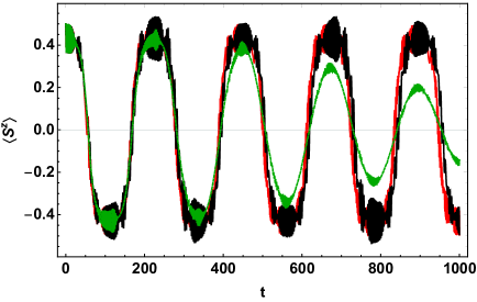
Figure 8: Comparison between the exact Hierarchy of correlations (black), its lowest order approximation using dRG (red) and the exact dynamics for the central spin (green), at long times. Parameters: $\Delta/B=0.03$, $J/B=0.05$ and $N=100$ for the initial condition $\langle S^{z}\left(0\right)\rangle=\frac{1}{2}$ and $\langle P_{z}\left(0\right)\rangle=N/2$.

Finally, Fig.9 shows the solutions from the flow equations for the cross-correlator between central spin and bath, and the magnetization components $M_{x,z}\left(t\right)$. It is interesting to see that the periodicity of the flow equations happens at quite long time (of the order of $t\sim 220$ in units of $B_{\perp}^{-1}$) and that the cross-correlator initial condition $a_{zy}\left(t\right)$ has large corrections, even when the system starts in an uncorrelated state (corrections of the order of $\sim B_{\perp}$ rather than $A_{i}$ or $\Delta_{\perp}$, which is what one would find in absence of renormalization). This means that central spin and bath become highly correlated and these correlations are needed for a correct description of the dynamics at late time.

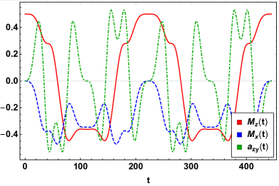
Figure 9: Numerical solution of the flow equations for the running of the different initial conditions. (Red, solid line) $M_{z}\left(t\right)$ still displays instanton-like behavior, but the profile is modified due to correlations with respect to the uncorrelated case (see Fig.6, red-dashed line). (Blue, dashed line) $M_{x}\left(t\right)$ also shows large corrections but it is always negative, which is expected due to the positive value chosen for the interaction parameter. (Green, dot-dashed line) $a_{zy}\left(t\right)$ displays complicated oscillations, correlated with the bath and the central spin magnetization, but importantly, acquires large values that can largely modify the mean field dynamics.