Length Spectrum Rigidity for Piecewise Analytic Bunimovich Billiards

Abstract

In the paper, we establish Squash Rigidity Theorem - the dynamical spectral rigidity for piecewise analytic Bunimovich squash-type stadia whose convex arcs are homothetic. We also establish Stadium Rigidity Theorem - the dynamical spectral rigidity for piecewise analytic Bunimovich stadia whose flat boundaries are a priori fixed.

In addition, for smooth Bunimovich squash-type stadia we compute the Lyapunov exponents along the maximal period two orbit, as well as the value of the Peierls’ Barrier function from the maximal marked length spectrum associated to the rotation number $\frac{2n}{4n+1}$.

1 Introduction

1.1 Background and Notations

A natural question is to understand what information on the geometry of the billiard table is encoded by the length spectrum, i.e., the set of lengths of periodic orbits. Motivated by the famous question of M. Kac [19]: “Can one hear the shape of a drum?”, which is formally called Laplace inverse spectral problem, we propose the following question from the perspective of billiard dynamics: is the knowledge of length spectrum sufficient to reconstruct the shape of the billiard table and hence the whole dynamics? We refer to this problem as the dynamical inverse spectral problem.

Both inverse spectral problems turn out to be extremely challenging, and only little progress have been achieved for some classes of convex billiards. On the one hand, the celebrated work [28, 29, 30] by Zelditch shows that the Laplace inverse spectral problem has a positive answer in the case on a generic class of analytic $\mathbb{Z}_{2}$-symmetric planar strictly convex domains. Hezari-Zelditch [15] have obtained a higher dimensional analogue of this result. Very recently, Hezari-Zelditch [17] showed that nearly circular ellipses are spectrally determined among all smooth domains, without assuming any symmetry, convexity, or closeness to the ellipse, on the class of domains. On the other hand, Colin de Verdière [5] had shown that the marked length spectrum determines completely the geometry of convex analytic billiards which have the symmetries of an ellipse. In the non-analytic situation, De Simoi, Kaloshin and Wei [9] have proven the length spectral rigidity, i.e., in the class of sufficiently smooth $\mathbb{Z}_{2}$-symmetric strictly convex table sufficiently close to a circle all deformations preserving the length spectrum are isometries. However, there are a number of counter-examples to the inverse spectral problem (see. e.g. [10, 25]), while the billiard domains in these examples are neither smooth nor strictly convex. To this end, great interest has been raised to see if the inverse spectral problem holds for a certain family of non-smooth non-convex billiards.

In this paper, we shall consider a class of Bunimovich billiard tables, which are not smooth at several boundary points. Moreover, these tables are not strictly convex. We would like to stress the dynamics on the Bunimovich billiards is significantly different from the elliptic dynamics on strictly convex billiards, that is, the billiard ball motion in Bunimovich tables exhibits hyperbolic behavior, accompanied with strong chaotic behavior and also have singularities. Here, we are able to obtain the spectral rigidity results for the first class of hyperbolic billiards with singularities. It is worth mentioning some recent results in [1, 8], where marked length spectral rigidity is shown for some open sets of hyperbolic billiards, whose dynamics are uniformly hyperbolic and can be coded by subshifts of finite type. Nevertheless, the Bunimovich billiards are non-uniformly hyperbolic and cannot be conjugate to symbolic systems on finite alphabet set. It was recently shown in [3] the induced systems of Bunimovich billiards are conjugate to a positive recurrent countable Markov shift with respect to the SRB measure. Hence the methods in [1, 8] cannot be directly applied for our setting.

In what follows, we describe the class of Bunimovich billiards and their dynamics. More precisely, we investigate two classes of billiards tables satisfying the following assumptions:

Assumption I

• A Bunimovich stadium $\Omega$ is a domain whose boundary $\partial\Omega$ is made of two $C^{3}$ strictly convex arcs $\Gamma_{1}$ and $\Gamma_{2}$, as well as two flat parallel boundaries $\Gamma_{3}$ and $\Gamma_{4}$, which are two opposite sides of a rectangle (see Fig. 1, left).

• A Bunimovich squash-type stadium $\Omega$ is a domain whose boundary $\partial\Omega$ is made of two $C^{3}$ strictly convex arcs $\Gamma_{1}$ and $\Gamma_{2}$, as well as two flat boundaries $\Gamma_{3}$ and $\Gamma_{4}$, which may not be parallel (see Fig. 1, middle).

Assumption II

In both cases ($\mathrm{I_{s}}$) and ($\mathrm{I_{ss}}$), we require that $\partial\Omega$ is $C^{1}$ but not $C^{2}$ smooth at each gluing point $\Gamma_{i}\cap\Gamma_{j}$, where $i=1,2$ and $j=3,4$.

Assumption III

• A Bunimovich stadium $\Omega$ satisfies the defocusing mechanism, i.e., for any $P_{1}\in\Gamma_{1}$ and $P_{2}\in\Gamma_{2}$,

  $$\left|\overline{P_{1}P_{2}}\right|>\max\left\{\left|\overline{P_{1}Q_{1}}\right|,\ \left|\overline{P_{2}Q_{2}}\right|\right\},$$ (1.1)

  where $Q_{i}$ is the other intersection point between the line passing through $P_{1},P_{2}$ and the osculating circle of $\Gamma_{i}$ at $P_{i}$, $i=1,2$ (see Fig. 1, left).

• For a Bunimovich squash-type stadiam $\Omega$, let $\widetilde{\Omega}$ be the double cover table by attaching a symmetric copy to $\Omega$ along $\Gamma_{3}$ or $\Gamma_{4}$, and let $\widetilde{\Gamma}_{1}$ and $\widetilde{\Gamma}_{2}$ be the two new arcs of $\widetilde{\Omega}$. A slightly stronger condition is required for a Bunimovich squash-type stadium $\Omega$: it satisfies the doubly defocusing mechanism, that is, (1.1) holds for any $P_{1}\in\Gamma_{1}\cup\widetilde{\Gamma}_{1}$ and $P_{2}\in\Gamma_{2}\cup\widetilde{\Gamma}_{2}$ (see Fig. 1, middle and right).

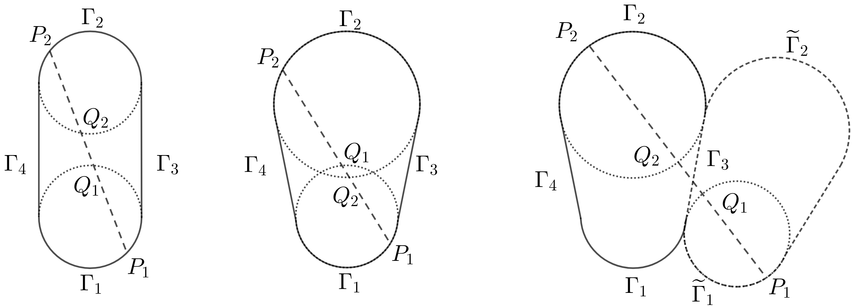
Figure 1: Bunimovich (squash-type) stadia and the (doubly) defocusing

Note that the class of the Bunimovich (squash-type) stadia is a generalization of the standard Bunimovich (squash) stadia, which is formed by circular arcs $\Gamma_{1}$ and $\Gamma_{2}$. We remark that the mechanism of (doubly) defocusing is robust for Bunimovich (squash-type) stadia under $C^{3}$ perturbations of $\Gamma_{1}$ and $\Gamma_{2}$.

It will be shown in Section 3 that under Assumptions ($\mathrm{I}$)-($\mathrm{III}$), any Bunimovich (squash-type) stadium $\Omega$ possesses a unique maximal period two orbit $\gamma^{*}=\overline{AB}$, where $A\in\Gamma_{1}$ and $B\in\Gamma_{2}$. The following condition is further assumed for the Bunimovich squash-type stadia.

Assumption IV

Let $\chi$ be a positive constant. A Bunimovich squash-type stadium $\Omega$ is said to be $\chi$-homethetic near the period two orbit $\gamma^{*}=\overline{AB}$ if there exists an orientation preserving linear transformation $\mathcal{S}:{\mathbb{R}}^{2}\to{\mathbb{R}}^{2}$ such that

• $\mathcal{S}$ is a homothety with ratio $\chi$, i.e.,

  $$\left|\mathcal{S}(v_{1})-\mathcal{S}(v_{2})\right|=\chi|v_{1}-v_{2}|\ \ \text{for any}\ v_{1},v_{2}\in{\mathbb{R}}^{2}.$$

• $\mathcal{S}(A)=B$ and $\mathcal{S}\left(\widehat{\Gamma}_{1}\right)=\widehat{\Gamma}_{2}$, where $\widehat{\Gamma}_{1}$ is a sub-curve of $\Gamma_{1}$ containing $A$ and $\widehat{\Gamma}_{2}$ is a sub-curve of $\Gamma_{2}$ containing $B$.

We stress that Assumption (IV) will only be imposed for the Bunimovich squash-type stadia. We shall call the constant $\chi$ the homothety ratio. Note that if $\chi=1$, then the two arcs $\Gamma_{1}$ and $\Gamma_{2}$ are locally isometric near $\gamma^{*}=\overline{AB}$.

To describe the billiard dynamics on the table $\Omega$, we assume the billiard ball moves at a unit speed, and the boundary $\partial\Omega$ is oriented in the counter-clockwise direction. Set $R=\left|\partial\Omega\right|$. The phase space is a cylinder given by

$$M:=\left\{(r,\varphi)\,:\,r\in[0,R]/\{0\sim R\},\ \varphi\in[-\pi/2,\pi/2]\right\},$$ (1.2)

where $r$ is an arclength parameter of $\partial\Omega$ and $\varphi$ is the angle formed by the collision vector and the inward normal vector of the boundary. We denote by $\tau(z,z_{1})$ the length of the free path of a billiard trajectory connecting $z=(r,\varphi)$ and $z_{1}=(r_{1},\varphi_{1})$ in $M$, and we also denote by

$$F:M\to M,\qquad F:(r,\varphi)\to(r_{1},\varphi_{1})$$

the associated billiard map.

Given any $q$-periodic billiard orbit $\gamma=\overline{z_{1}z_{2}\dots z_{q}}$, i.e., $Fz_{i}=z_{i+1}$ for $1\leq i\leq q-1$ and $Fz_{q}=z_{1}$, we set $z_{k}=z_{i}$ if $k\equiv i\pmod{q}$. The total length for the periodic orbit $\gamma$ is given by

$$L(\gamma):=\sum_{i=1}^{q}\tau(z_{i},z_{i+1}).$$ (1.3)

The winding number $p$ of a $q$-periodic orbit $\gamma$ measures how many times the orbit $\gamma$ goes around $\partial\Omega$ along the counter-clockwise direction until it comes back to the starting point. The rotation number of a $q$-periodic orbit $\gamma$ is given by $\rho(\gamma):=p/q$, where $p\geq 1$ is the winding number of $\gamma$. Due to time reversibility, we study only $p/q\in{\mathbb{Q}}\cap(0,1/2]$. We denote the set of periodic orbits of rotation number $p/q$, by $\Gamma_{p/q}$.

We introduce the length spectrum of a billiard table $\Omega$ as the set of lengths of all periodic orbits, counted with multiplicity:

$$\mathcal{L}(\Omega):={\mathbb{N}}\cdot\{L(\gamma)\,|\,\gamma\text{ is a periodic billiard orbit }\}\ \cup\ {\mathbb{N}}\cdot\{|\partial\Omega|\}.$$

One difficulty working with the length spectrum $\mathcal{L}(\Omega)$ is that its (length) elements have no labels, e.g. rotation numbers of the associate periodic orbits. One possibility is to consider the so-called maximal marked length spectrum as in [12] (see also [23] and [22]), by associating to each length the corresponding rotation number. More precisely, we consider a map $\mathcal{ML}_{\Omega}^{\max}:\mathbb{Q}\cap(0,1/2]\to\mathbb{R}^{+}$ such that for any $p/q\in\mathbb{Q}\cap(0,1/2]$ in lowest terms,

$$\mathcal{ML}_{\Omega}^{\max}(p/q)=\max\{L(\gamma)|\,\,\gamma\in\Gamma_{p/q}\}.$$ (1.4)

We say that a periodic orbit $\gamma$ is maximal of rotation number $p/q$ if $\rho(\gamma)=p/q$ and $L(\gamma)=\mathcal{ML}^{\max}_{\Omega}(p/q)$.

1.2 Motivation and the Main Results

A natural question is

If two Bunimovich (squash-type) stadia have the same (marked) length spectra, are these two tables isometric?

In the case of geodesic flows on hyperbolic surfaces (Riemannian surfaces of negative curvature) the affirmative answer was obtained independently by Otal [21] and Croke [6]. Later on, Croke-Sharafutdinov [7] proved the Laplace spectral rigidity of compact negatively curved manifolds, and later Guillarmou-Lefeuvre [11] proved a local version of the marked length spectral rigidity for Anosov manifolds. It is well-known that geodesic flows on hyperbolic surfaces is uniformly hyperbolic and, as the result, has strong chaotic properties, e.g. the number of periodic orbits of period up to $T$ growth exponentially with $T$. Bunimovich squash-type stadia also represent billiards with strongly chaotic properties and is an analog of geodesic flows on hyperbolic surfaces. In this paper we obtain the geometric information about the underlying stadium from its (Marked) Length Spectrum. In particular, our results only depend on the length spectrum of periodic orbits near a period two orbit, see below for details.

1.2.1 Dynamical spectral rigidity for piecewise analytic domains

Our first main result concerns the dynamical length spectrum rigidity for the Bunimovich (squash-type) stadia.

Let $\mathcal{M}$ be a space of domains and $\left\{\Omega_{\mu}\right\}_{|\mu|\leq 1}$ be a $C^{1}$ one-parameter family in $\mathcal{M}$. The family $\left\{\Omega_{\mu}\right\}_{|\mu|\leq 1}$ is called dynamically isospectral if the length spectra are identical for each $\mu$, i.e., $\mathcal{L}(\Omega_{0})=\mathcal{L}(\Omega_{\mu})$ for any $\mu\in[-1,1]$. A domain $\Omega\in\mathcal{M}$ is dynamically spectrally rigid in $\mathcal{M}$ if for any $C^{1}$ one-parameter family $\left\{\Omega_{\mu}\right\}_{|\mu|\leq 1}$ in $\mathcal{M}$ with $\Omega_{0}=\Omega$ we have

$$\left\{\Omega_{\mu}\right\}_{|\mu|\leq 1}\ \text{ is \ dynamically\ isospectral }\Longrightarrow\ \Omega_{\mu}\cong\Omega\ \text{for any}\ \mu\in[-1,1].$$

Here $\Omega_{\mu}\cong\Omega$ means that $\left\{\Omega_{\mu}\right\}_{|\mu|\leq 1}$ is an isometric family, i.e., there exists a family $\left\{\mathcal{T}_{\mu}\right\}_{|\mu|\leq 1}$ of planar isometries such that $\Omega_{\mu}=\mathcal{T}_{\mu}\Omega$. We also say that $\left\{\Omega_{\mu}\right\}_{|\mu|\leq 1}$ is a constant family if $\Omega_{\mu}=\Omega$ for all $\mu\in[-1,1]$.

Let $\mathcal{M}^{\omega}_{ss}$ (resp. $\mathcal{M}^{m}_{ss}$ with $m\geq 3$) be the space of Bunimovich squash-type stadia $\Omega$ such that $\Omega$ satisfies Assumptions $\mathrm{(I_{ss})(II)(III_{ss})}$ and the convex arcs $\Gamma_{1}$ and $\Gamma_{2}$ are analytic (resp. $C^{m}$ smooth) curves. Moreover, given $\chi>0$, we let $\mathcal{M}^{\omega}_{ss}(\chi)$ (resp. $\mathcal{M}^{m}_{ss}(\chi)$ with $m\geq 3$) be the subspace of $\mathcal{M}^{\omega}_{ss}$ (resp. $\mathcal{M}^{m}_{ss}$ with $m\geq 3$) in which the Bunimovich squash-type stadia satisfy Assumption (IV) with homothety ratio $\chi$.

In the analytic space $\mathcal{M}^{\omega}_{ss}$ it is somewhat unconventional to have all four parts $\Gamma_{j},\ j=1,2,3,4$, analytic and at the same time have Assumption (II) which requires that at the gluing points the boundary is $C^{1}$, but not $C^{2}$. This condition will be used in the proof of Lemma 5.2, which is crucial to the proof of the dynamical spectral rigidity for the Bunimovich squash-type stadia.

Our first main result is the following.

Squash Rigidity Theorem.

For any $\chi>0$, a Bunimovich squash-type stadium $\Omega\in\mathcal{M}^{\omega}_{ss}(\chi)$ is dynamically spectrally rigid in $\mathcal{M}^{\omega}_{ss}(\chi)$.

Important progress have been recently made for spectral rigidity of convex billiard tables. Our result is similar to [9], in which De Simoi, Kaloshin and Wei established the dynamical spectral rigidity for a class of finitely smooth strictly convex ${\mathbb{Z}}_{2}$ symmetric domains sufficiently close to the circle. On the other hand, the Laplacian spectral rigidity was proved by Hezari and Zelditch [16] for a one-parameter $C^{\infty}$ domains that preserve the ${\mathbb{Z}}_{2}\times{\mathbb{Z}}_{2}$ symmetry group of ellipse. For the same class of domains in [9], Hezari [14] showed the Laplacian spectral rigidity under the Robin boundary condition. A three disk model with ${\mathbb{Z}}_{2}\times{\mathbb{Z}}_{2}$-symmetry and analytic boundary was considered in [8], which showed that Marked Length Spectrum uniquely determined the boundary. This result is analogous to well-known results of Zeldich [29, 30].

Note that for any Bunimovich squash-type stadium $\Omega\in\mathcal{M}_{ss}^{m}$ with $m\geq 3$, there is a unique maximal period two orbit $\gamma^{*}=\overline{AB}$ (see Section 3). In the proof of Squash Rigidity Theorem, we actually show the flatness of the deformation function $\mathbf{n}$ (see (5.1) for the definition) at the period two orbit $\gamma^{*}$, which holds for the normalized family of Bunimovich squash-type stadia not only in $\mathcal{M}^{\omega}_{ss}(\chi)$ but also in $\mathcal{M}^{\infty}_{ss}(\chi)$ (see Proposition 6.2).

Theorem 1.

For any $\Omega\in\mathcal{M}^{\infty}_{ss}(\chi)$ with some $\chi>0$ and for any $C^{1}$ one-parameter normalized family of dynamically isospectral domains $\left\{\Omega_{\mu}\right\}_{|\mu|\leq 1}$ in $\mathcal{M}^{\infty}_{ss}(\chi)$ with $\Omega_{0}=\Omega$, we have

$$\mathbf{n}^{(d)}(A)=\mathbf{n}^{(d)}(B)=0,\ \ \text{for any}\ d\geq 0.$$

We remark that our Theorem 1 implies that the deformation function $\mathbf{n}\equiv 0$ in the analytic case. Observe that in Corollary 1 of [16], a flat dependence on $\mu$ is proven. In the analytic setting it leads to absence of non-trivial real analytic deformation. We note that a similar problem of analysing periodic orbits approximating a period two orbit was studied in [27]. However, the proof is different here, because of the existence of singularity for billiards.

We provide the brief ideas and main steps on how to obtain our Theorem 1, which asserts the Taylor coefficients of the deformation function $\mathbf{n}$ are all vanishing at the period two orbit $\gamma^{*}$.

• In Section 3 we analyse the dynamical properties of the period two orbit $\gamma^{*}$, and then in Section 4, we construct a sequence of palindromic periodic orbits $\gamma_{n}$ such that the limiting semi-orbit $\gamma_{\infty}$ is homoclinic to the period two orbit $\gamma^{*}$. Using the special properties of the palindromic orbits, we obtain quantitative estimates for the coordinates of $\gamma_{n}$ near $\gamma^{*}$ when $k\approx n/2$ (see Lemma 4.4 and Remark 4.5), as well as estimates for the shadowing of $\gamma_{n}$ along the homoclinic semi-orbit $\gamma_{\infty}$ (see Lemma 4.6) .

• In Section 5 we study the Linearized Isospectral Functionals related to the special orbits. Following the work of [9], we obtain the special function $G(r,\varphi)=\mathbf{n}(r)\cos\varphi$ must have vanishing periodic data for a dynamical isospectral family. In particular, the sum of $G$ over the special orbits $\gamma^{*}$ and $\gamma_{n}$ must be zero.

• In Section 6 we study the sum of $G$ over the palindromic orbit $\gamma_{n}$ by separate it into two sums: one is a global sum $S_{n}^{global}(\ell)$ (with minus sign) away from the period two orbit $\gamma^{*}$, the other is the local sum $S_{n}^{local}(\ell)$ near $\gamma^{*}$. As the total sum is vanishing, we must have $S_{n}(\ell)=S_{n}^{global}(\ell)=S_{n}^{local}(\ell)$. In other words, we define a sum $S_{n}(\ell)$ over $\gamma_{n}$ which has two representations (see Subsection 6.2.1).

  • For the global sum: by Lemma 4.6, when $k\leq\ell$, the points $x_{2\ell+j}(k)$ on the palindromic orbit $\gamma_{2\ell+j}(k)$ lie on an asymptotic line through $\gamma_{\infty}(k)$, which have asymptotic geometric spacing of order $\lambda^{-j}$. Due to this observation, we can perform the Lagrange interpolation method, either the classical or the weighted one, to make a linear cancellation for the global sum representation, i.e., we show that a linear combination of $\{S_{2\ell+j}\}_{0\leq j\leq m}$ must vanish up to a higher order (see Lemma 6.6).

  • For the local sum: we can write down the Taylor expansions for the local representation of $S_{n}(\ell)$. Suppose that the lowest non-vanishing degree of $\mathbf{n}$ is $d$. Using the linear cancellation that we have obtained in Lemma 6.6, we further obtain a linear equation with two variables $\mathbf{n}^{(d)}(A)$ and $\mathbf{n}^{(d)}(B)$, which further implies that $\mathbf{n}^{(d)}(A)=\mathbf{n}^{(d)}(B)=0$ by Assumption (IV).

Note that Squash Rigidity Theorem is then a direct consequence of Theorem 1, due to the analyticity of boundary of Bunimovich squash-type stadia in $\mathcal{M}^{\omega}_{ss}$.

We also consider special Bunimovich stadia whose flat boundaries are a priori fixed. To be precise, let $\Gamma_{3}$ and $\Gamma_{4}$ be the opposite sides of a fixed rectangle. We then denote by $\mathcal{M}^{\omega}_{s,b}$ (resp. $\mathcal{M}^{m}_{s,b}$ with $m\geq 3$) the space of Bunimovich stadia $\Omega$ such that $\Omega$ satisfies Assumptions $\mathrm{(I_{s})(II)}$, the convex arcs $\Gamma_{1}$ and $\Gamma_{2}$ are analytic curves (resp. $C^{m}$ curves), and the flat boundaries are exactly $\Gamma_{3}$ and $\Gamma_{4}$. We remark that Assumption $\mathrm{(III_{s})}$ - the defocusing mechanism and Assumption (IV) - the homothetic condition are not required for the Bunimovich stadia in $\mathcal{M}^{\omega}_{s,b}$ (resp. $\mathcal{M}^{m}_{s,b}$ with $m\geq 3$). Using the unfolding trick, we provide a simpler but quite different proof for the dynamical spectral rigidity for the class $\mathcal{M}^{\omega}_{s,b}$. Namely, our second main result is stated as follows.

Stadium Rigidity Theorem.

A Bunimovich stadium $\Omega\in\mathcal{M}^{\omega}_{s,b}$ is dynamically spectrally rigid in $\mathcal{M}^{\omega}_{s,b}$.

The core in the proof of Stadium Rigidity Theorem is again flatness of the deformation function, but at the four gluing points, i.e. $P_{ij}:=\Gamma_{i}\cap\Gamma_{j},\ \ i=1,2,\ j=3,4.$ (see Proposition 7.3 for the precise statements).

Theorem 2.

For any $\Omega\in\mathcal{M}^{\infty}_{s,b}$ and any $C^{1}$ one-parameter family of dynamically isospectral domains $\left\{\Omega_{\mu}\right\}_{|\mu|\leq 1}$ in $\mathcal{M}^{\infty}_{s,b}$ with $\Omega_{0}=\Omega$, we have

$$\mathbf{n}^{(d)}(P)=0,\ \ \text{for any}\ d\geq 0\ \text{ and any gluing point }P\ \text{of}\ \Omega.$$

Here $\mathbf{n}^{(d)}(P)$ denotes the one-sided $d$-th order derivative defined on the part of convex arc $\Gamma_{1}$ or $\Gamma_{2}$.

In the proof of Theorem 2, we shall construct some special orbits of induced period two and four (see Lemma 7.1 and Lemma 7.2), which are sufficient to compute the Taylor expansion of the deformation function $\mathbf{n}$ near the gluing points. The arguments there do not require the hyperbolicity at all, which is why we can drop the defocusing mechanism.

1.2.2 Marked length spectrum

Recall that $\gamma^{*}=\overline{AB}$ is the maximal period two orbit, which bounces between $\Gamma_{1}$ and $\Gamma_{2}$. It is clear that the rotation number of $\gamma^{*}$ is $\frac{1}{2}$. Denote the free path $\tau^{*}=\tau(A,B):=\left|\overline{AB}\right|$, and note that $\tau^{*}={\rm diam}(\Omega)$.

Our third main result demonstrates the marked length spectrum provides information about the Lyapunov exponents along the maximal period two orbit $\gamma^{*}$.

Theorem 3.

Let $\Omega$ be a Bunimovich squash-type stadium in $\mathcal{M}^{m}_{ss}$ for $m\geq 3$. Then with notations (1.4) the following limits exist:

$$\begin{split}-B_{\frac{1}{2}}&:=\lim_{n\to\infty}\left[\mathcal{ML}^{\max}_{\Omega}\left(\frac{2n}{2n+1}\right)-(2n+1)\tau^{*}\right],\\ -\log\lambda&:=\,\lim_{n\to\infty}\frac{1}{n}\log\left|\mathcal{ML}^{\max}_{\Omega}\left(\frac{2n}{2n+1}\right)-(2n+1)\tau^{*}+B_{\frac{1}{2}}\right|,\\ D_{\frac{1}{2}}&:=\lim_{n\to\infty}\lambda^{n}\left|\mathcal{ML}^{\max}_{\Omega}\left(\frac{2n}{2n+1}\right)-(2n+1)\tau^{*}+B_{\frac{1}{2}}\right|.\end{split}$$

The above theorem for Bunimovich squash-type stadia is similar to results for strictly convex billiards in [18]. A somewhat similar computation has been done for dispersing billiards in [1]. In the Aubry-Mather theory, $B_{\frac{1}{2}}$ is usually referred to the Peierls’ Barrier function evaluated on a certain homoclinic orbit of $\gamma^{*}$, and $\lambda$ is the eigenvalue of the linearization of the billiard map along $\gamma^{*}$. In the proof of Theorem 3, we show that the quantity $B_{\frac{1}{2}}$ is finite, and the convergence of (3) is exponentially fast.

Plan of the paper:  The rest of the paper is organized as follows. In Section 2 we present auxiliary facts about the billiard map and properties of the billiard dynamics near the unique period two orbit. In Section 3 we study the billiard dynamics in a neighborhood of the maximal period two orbit $\gamma^{*}$. In Section 4 we analyze the palindromic periodic orbits approximating the period two orbit $\gamma^{*}$. In Section 5 we define linearized isospectral functionals related to some special periodic orbits, whose properties are closely related to dynamical spectral rigidity. In Section 6 utilizing properties of approximating palindromic periodic orbits we prove Squash Rigidity Theorem. In Section 7 using a different approach we prove Stadium Rigidity Theorem. Finally, in Section 8 we analyze the periodic orbits with rotation number $\pm\frac{n}{2n+1}$ and obtain shadowing estimates similar to Section 4. Then in Section 9 we prove Theorem 3 about Lyapunov exponents of the maximal period two orbit.

Acknowledgement VK acknowledges a partial support by the NSF grant DMS-1402164. Discussions with Martin Leguil and Jacopo De Simoi were very useful. The authors would like to thank a referee for pointing out a mistake in a preliminary version of the paper. It led to a more restrictive (homothetic) rigidity for squash stadia. JC was partially supported by NSFC grant 12001392 and NSF of Jiangsu BK20200850. H.-K. Zhang is partially supported by Simons Foundation Collaboration Grants for Mathematicians (Grant No.706383).

2 The Billiard Dynamics

2.1 The Billiard Map and Its Differential

Let $\Omega$ be a Bunimovich squash-type stadium. We recall that the phase space $M$ has the form

$$M=\left\{x=(r,\varphi)\,:\,0\leq r\leq\left|\partial\Omega\right|,\ \ \varphi\in\left[-\pi/2,\pi/2\right]\right\}.$$

and the billiard map $F:M\to M$ sends $z=(r,\varphi)$ to $z_{1}=(r_{1},\varphi_{1})$. The free path between $z$ and $z_{1}$ is given by $\tau=\tau(z,z_{1})=\left|\overline{PP_{1}}\right|$, where $P$ and $P_{1}$ be the collision points at $\partial\Omega$ corresponding to $z$ and $z_{1}$ respectively. The derivative $D_{z}F$ is given by

$$\begin{pmatrix}dr_{1}\\ d\varphi_{1}\end{pmatrix}=\frac{-1}{\cos\varphi_{1}}\begin{pmatrix}\tau\mathcal{K}+\cos\varphi&\tau\\ \tau\mathcal{K}\mathcal{K}_{1}+\mathcal{K}\cos\varphi_{1}+\mathcal{K}_{1}\cos\varphi&\tau\mathcal{K}_{1}+\cos\varphi_{1}\end{pmatrix}\begin{pmatrix}dr\\ d\varphi\end{pmatrix},$$ (2.1)

where $\mathcal{K}=\mathcal{K}(z)$ and $\mathcal{K}_{1}=\mathcal{K}(z_{1})$ are the signed curvature of $\partial\Omega$ at $P$ and $P_{1}$ respectively (see Section 2.11 in [4]). In particular, $\mathcal{K}(z)$ is negative if $P$ belongs to the convex arcs $\Gamma_{1}\cup\Gamma_{2}$.

2.2 Wave Fronts and Unstable Curves

We recall some basic notions and formulae in [4]. Given a tangent vector $dz=(dr,d\varphi)\in T_{z}M$, we denote by $\|dz\|=\sqrt{dr^{2}+d\varphi^{2}}$ the Euclidean norm and by $\|dz\|_{p}=\cos\varphi|dr|$ the $p$-norm. The tangent vector $dz$ corresponds to a tangent line with slope $\mathcal{V}=d\varphi/dr$ in $T_{z}M$, as well as a pre-collisional wave front with slope $\mathcal{B}^{-}$ and post-collisional wave front with slope $\mathcal{B}^{+}$ in the phase space of the billiard flow. The relation between these slopes are given by

$$\mathcal{V}=\mathcal{B}^{-}\cos\varphi+\mathcal{K}=\mathcal{B}^{+}\cos\varphi-\mathcal{K}.$$

For any $z=(r,\varphi)\in M$ lying on the convex arcs $\Gamma_{1}\cup\Gamma_{2}$, the $DF$-invariant unstable cones is given by

$$\mathcal{C}^{u}(z)=\left\{\mathcal{K}\leq\mathcal{V}\leq 0\right\}=\left\{0\leq\mathcal{B}^{-}\leq 1/d\right\}=\left\{-2/d\leq\mathcal{B}^{+}\leq-1/d\right\}.$$

where $\mathcal{K}=\mathcal{K}(z)<0$ and $d=-\cos\varphi/\mathcal{K}$. By the defocusing mechanism and the compactness of $\Gamma_{1}\cup\Gamma_{2}$, there exists $\rho_{0}>1$ such that

• $\tau=\tau(z,z_{1})\geq 2\rho_{0}d$ if $z$ lies on $\Gamma_{1}$ and $z_{1}=F(z)$ lies on $\Gamma_{2}$, or vice versa;

• if further the doubly defocusing mechanism holds, and $z$ lies on $\Gamma_{1}$ (resp. on $\Gamma_{2}$), $z^{\prime}=F(z)$ lies on $\Gamma_{3}$ but $z_{1}=F^{2}(z)$ lies on $\Gamma_{2}$ (resp. on $\Gamma_{1}$), then

  $$\tau=\widetilde{\tau}(z,\widetilde{z}_{1})\geq 2\rho_{0}d,$$

  where $\widetilde{\tau}(\cdot,\cdot)$ is the free path for the double cover table $\widetilde{\Omega}$ (see Fig. 1, right), and $\widetilde{z}_{1}$ is symmetric to $z_{1}$ with respect to $\Gamma_{3}$.

In either case, if $dz\in\mathcal{C}^{u}(z)$, then $dz_{1}\in\mathcal{C}^{u}(z_{1})$ and

$$\frac{\|dz_{1}\|_{p}}{\|dz\|_{p}}=\frac{\left|\mathcal{B}^{+}\right|}{\left|\mathcal{B}^{-}_{1}\right|}=\left|1+\tau\mathcal{B}^{+}\right|=-1-\tau\mathcal{B}^{+}\geq 2\rho_{0}-1=:\Lambda>1.$$ (2.2)

Given a smooth curve $W$ in $M$, we denote its Euclidean length and $p$-length by

$$|W|=\int_{W}\|dz\|,\ \text{and}\ \ |W|_{p}=\int_{W}\|dz\|_{p}.$$

If it is an unstable curve, i.e., $d\varphi/dr\in\mathcal{C}^{u}(z)$ for any $z=(r,\varphi)\in W$, then $F(W)$ (resp. $F^{2}(W)$) is an unstable curve in the above case (i) (resp. case (ii)), as long as it does not hit the gluing points. Moreover, we have

$$|F(W)|_{p}\geq\Lambda|W|_{p}\ \text{in case (i), \ or}\ |F^{2}(W)|_{p}\geq\Lambda|W|_{p}\ \text{in case (ii)}.$$ (2.3)

2.3 Variation of a Free Path

In the above notations the billiard map $F$ sends $z=(r,\varphi)$ to $z_{1}=(r_{1},\varphi_{1})$. Note that if $r$ and $r_{1}$ are given, then $\varphi$ and $\varphi_{1}$ are uniquely determined. As the free path $\tau=\tau(z,z_{1})$ is only determined by $r$ and $r_{1}$, we also write $\tau=\tau(r,r_{1})$. Elementary geometry shows that

$$\frac{\partial\tau}{\partial r}=-\sin\varphi\quad\ \ \text{and}\quad\ \ \frac{\partial\tau}{\partial r_{1}}=\sin\varphi_{1}.$$ (2.4)

The following lemma provides a variational formula of a free path.

Lemma 2.1.

The variation, from $\tau(r,r_{1})$ to $\tau(r+\Delta r,r_{1}+\Delta r_{1})$, has the form:

$$\Delta\tau = \tau(r+\Delta r,r_{1}+\Delta r_{1})-\tau(r,r_{1})$$ (2.5)

$$= -\sin\varphi\ \Delta r+\sin\varphi_{1}\ \Delta r_{1}$$

$$+\frac{1}{2}\left[\alpha(z)\Delta r^{2}+\beta(z,z_{1})\Delta r\Delta r_{1}+\alpha(z_{1})\Delta r_{1}^{2}\right]$$

$$+\mathcal{O}\left(\left(\Delta r^{2}+\Delta r_{1}^{2}\right)^{\frac{3}{2}}\right),$$

$$\text{with}\ \ \alpha(z)=\mathcal{K}\cos\varphi+\frac{\cos^{2}\varphi}{\tau},\alpha(z_{1})=\mathcal{K}_{1}\cos\varphi_{1}+\frac{\cos^{2}\varphi_{1}}{\tau}\ \ \text{and}\ \ \beta(z,z_{1})=\frac{2\cos\varphi\cos\varphi_{1}}{\tau},$$

where $\mathcal{K}$ and $\mathcal{K}_{1}$ are the signed curvatures of $\partial\Omega$ at $r$ and $r_{1}$ respectively.

Proof.

Taking $dr_{1}=0$ in (2.1), we obtain that

$$\frac{\partial\varphi}{\partial r}=-\mathcal{K}-\frac{\cos\varphi}{\tau},\ \ \text{and}\ \ \frac{\partial\varphi_{1}}{\partial r}=\frac{\cos\varphi}{\tau}.$$

By time-reversibility, i.e., $(r_{1},-\varphi_{1})\mapsto(r,-\varphi)$, we also have

$$\frac{\partial\varphi_{1}}{\partial r_{1}}=\mathcal{K}_{1}+\frac{\cos\varphi_{1}}{\tau},\ \ \text{and}\ \ \frac{\partial\varphi}{\partial r_{1}}=-\frac{\cos\varphi_{1}}{\tau}.$$

By (2.4), we further obtain

$$\frac{\partial^{2}\tau}{\partial r^{2}} = -\cos\varphi\frac{\partial\varphi}{\partial r}=\mathcal{K}\cos\varphi+\frac{\cos^{2}\varphi}{\tau},$$

$$\frac{\partial^{2}\tau}{\partial r\partial r_{1}} = -\cos\varphi\frac{\partial\varphi}{\partial r_{1}}=\frac{\cos\varphi\cos\varphi_{1}}{\tau},$$ (2.6)

$$\frac{\partial^{2}\tau}{\partial r_{1}^{2}} = \cos\varphi_{1}\frac{\partial\varphi_{1}}{\partial r_{1}}=\mathcal{K}_{1}\cos\varphi_{1}+\frac{\cos^{2}\varphi_{1}}{\tau}.$$

Therefore, (2.5) follows from (2.4) and (2.3), and the Taylor expansion of $\tau(x,x_{1})$ up to the second order. ∎

3 Analysis of the Period Two Orbit $\gamma^{*}$

3.1 Existence and Uniqueness of the Period Two Orbit $\gamma^{*}$

Let $\Omega$ be a Bunimovich squash-type stadium in $\mathcal{M}^{m}_{ss}$ for $m\geq 3$. The existence and uniqueness of the period two orbit, which bounces between $\Gamma_{1}$ and $\Gamma_{2}$, is due to the following lemma.

Lemma 3.1.

There exists a unique pair of points $(A,B)\in\Gamma_{1}\times\Gamma_{2}$ such that $\overline{AB}$ is perpendicular to both $\Gamma_{1}$ and $\Gamma_{2}$.

Proof.

Consider the free path $\tau=\tau(r,r_{1})$ for $(r,r_{1})\in\Gamma_{1}\times\Gamma_{2}$, and let $P$ and $P_{1}$ be the collision points corresponding to $r$ and $r_{1}$ respectively. Let $\varphi$ (resp. $\varphi_{1}$) be the angle formed by the vector $\overline{rr_{1}}$ and the inward (resp. outward) inner normal vector at $r$ (resp. at $r_{1}$). By (2.4), $\overline{PP_{1}}$ is perpendicular to both $\Gamma_{1}$ and $\Gamma_{2}$ if and only if $(r,r_{1})$ is a critical point of $\tau$. Moreover, by (2.3), the Hessian matrix of $\tau$ is given by

$$\begin{pmatrix}\mathcal{K}\cos\varphi+\dfrac{\cos^{2}\varphi}{\tau}&\dfrac{\cos\varphi\cos\varphi_{1}}{\tau}\\ \dfrac{\cos\varphi\cos\varphi_{1}}{\tau}&\mathcal{K}_{1}\cos\varphi_{1}+\dfrac{\cos^{2}\varphi_{1}}{\tau}\end{pmatrix}.$$

By the defocusing mechanism (1.1), we have $\mathcal{K}\tau<-2\cos\varphi$ and $\mathcal{K}_{1}\tau<-2\cos\varphi_{1}$, and thus the Hessian matrix of $\tau$ is negative definite since

$$\mathcal{K}\cos\varphi+\dfrac{\cos^{2}\varphi}{\tau}<-\dfrac{\cos^{2}\varphi}{\tau}<0,$$

and the determinant of Hessian is

$$\left(\mathcal{K}\cos\varphi+\dfrac{\cos^{2}\varphi}{\tau}\right)\left(\mathcal{K}_{1}\cos\varphi_{1}+\dfrac{\cos^{2}\varphi_{1}}{\tau}\right)-\dfrac{\cos^{2}\varphi\cos^{2}\varphi_{1}}{\tau^{2}}>0.$$

In other words, $\tau$ is a strictly concave function on $\Gamma_{1}\times\Gamma_{2}$, and thus there can be at most one critical point for $\tau$.

On the compact domain $\Gamma_{1}\times\Gamma_{2}$, $\tau$ has a global maximum point, say $(A,B)$. We claim that $(A,B)$ must be an interior point of $\Gamma_{1}\times\Gamma_{2}$. Otherwise, let $(r,r_{1})$ be the arclength representation of $(A,B)$, and assume that $r\in\partial\Gamma_{1}$. Since $\Gamma_{1}$ is $C^{1}$ tangent to flat boundaries at the gluing point, when $r+\Delta r\in\Gamma_{1}$ for small $\Delta r$, we must have $\varphi$ and $\Delta r$ are of opposite signs. By (2.4),

$$\tau(r+\Delta r,r_{1})=-\sin\varphi\Delta r+\mathcal{O}(|\Delta r|^{2})>0,$$

which implies that $(A,B)$ is not even a local maximum - Contradiction. Therefore, the global maximum point $(A,B)$ is an interior point and thus the only critical point of $\tau$ on $\Gamma_{1}\times\Gamma_{2}$. ∎

From the proof, we actually get $\tau^{*}=\tau(A,B)=|\overline{AB}|={\rm diam}(\Omega)$. In the rest of this section, we consider the maximal period two billiard orbit $\gamma^{*}=\overline{AB}$ that collides alternatively at $A\in\Gamma_{1}$ and $B\in\Gamma_{2}$.

3.2 Hyperbolicity of the Maximal Period Two Orbit $\gamma^{*}$

Since $\gamma^{*}=\overline{AB}$ is perpendicular to both $\Gamma_{1}$ and $\Gamma_{2}$, we denote $x=(r_{1},0)$ and $y=(r_{2},0)$ the collision vectors at $A$ and $B$ respectively, for some $0<r_{1}<r_{2}<\left|\partial\Omega\right|$. We shall also use the notation $\gamma^{*}=\overline{xy}$ for $\gamma^{*}=\overline{AB}$, and use the notation $\tau^{*}=\tau(x,y)$ for $\tau^{*}=\tau(A,B)$.

For convenience, we may choose $s$ as an arclength parameter on $\Gamma_{1}$ oriented in the counter-clockwise direction, with $s=0$ corresponding to the position of $A$. Similarly, we denote $t$ as a counter-clockwise arclength parameter on $\Gamma_{2}$ , with $t=0$ corresponding to the position of $B$.

Using the coordinate $(s,\varphi)$ on $\Gamma_{1}$ and $(t,\varphi)$ on $\Gamma_{2}$, the differential of the billiard map $F$ along $\gamma^{*}=\overline{xy}$ can be represented by the following matrices:

$$\begin{split}D_{x}F&=-\begin{pmatrix}1-\tau^{*}\mathcal{K}_{A}&\tau^{*}\\ \\ \tau^{*}\,\mathcal{K}_{A}\mathcal{K}_{B}-\mathcal{K}_{A}-\mathcal{K}_{B}&1-\tau^{*}\,\mathcal{K}_{B}\end{pmatrix}=:-\begin{pmatrix}a_{1}&\tau^{*}\\ b&a_{2}\end{pmatrix},\ \\ \ \ D_{y}F&=-\begin{pmatrix}a_{2}&\tau^{*}\\ b&a_{1}\end{pmatrix},\end{split}$$ (3.1)

where $\mathcal{K}_{A}$ and $\mathcal{K}_{B}$ are the absolute curvature of $\partial\Omega$ at $A$ and $B$ respectively. By the defocusing mechanism (1.1), we have $\tau^{*}>\max\{2/\mathcal{K}_{A},\ 2/\mathcal{K}_{B}\}$, which means that $a_{1}<-1$ and $a_{2}<-1$. Note that $a_{1}a_{2}-b\tau^{*}=1$. Hence

$$\begin{split}D_{x}F^{2}&=\begin{pmatrix}2a_{1}a_{2}-1&2a_{2}\tau^{*}\\ 2a_{1}b&2a_{1}a_{2}-1\end{pmatrix},\,\\ D_{y}F^{2}&=\begin{pmatrix}2a_{2}a_{1}-1&2a_{1}\tau^{*}\\ 2a_{2}b&2a_{1}a_{2}-1\end{pmatrix}\end{split}$$ (3.2)

are hyperbolic matrices since they have determinant one and the same trace

$$\lambda+\lambda^{-1}=2(2a_{1}a_{2}-1)>2,$$ (3.3)

where $\lambda$ denotes the leading eigenvalues of $D_{x}F^{2}$ (which is the same for $D_{y}F^{2}$). Therefore, $\gamma^{*}$ is a hyperbolic orbit.

The variation of the free path near $\gamma^{*}=\overline{xy}$ can be simplified as follows: if collision points move from $(s,t)=(0,0)$ to $(s,t)=(\Delta s,\Delta t)$, then (2.5) reads

$$\Delta\tau=\frac{1}{2\tau^{*}}\left[a_{1}\Delta s^{2}+2\Delta s\Delta t+a_{2}\Delta t^{2}\right]+\mathcal{O}\left(\left(\Delta s^{2}+\Delta t^{2}\right)^{\frac{3}{2}}\right),$$ (3.4)

where $a_{1}$ and $a_{2}$ are given by (3.1).

3.3 The Linearization near $\gamma^{*}$

We denote by $\theta_{1}^{s}$ (resp. $\theta_{1}^{u}$) the angle formed by the unit stable (resp. unstable) vector $V^{s}_{x}$ (resp. $V^{u}_{x}$) of $D_{x}F^{2}$ with the positive $r$-axis, then

$$V^{s}_{x}=(\cos\theta_{1}^{s},\sin\theta_{1}^{s})\quad\text{ and }\quad V^{u}_{x}=(\cos\theta_{1}^{u},\sin\theta_{1}^{u}).$$

Using (3.2) and the eigenvector equations:

$$\begin{split}(2a_{1}a_{2}-1-\lambda^{-1})\cos\theta_{1}^{s}+2a_{2}\tau^{*}\sin\theta_{1}^{s}&=0,\\ (2a_{1}a_{2}-1-\lambda)\cos\theta_{1}^{u}+2a_{2}\tau^{*}\sin\theta_{1}^{u}&=0,\end{split}$$

we obtain

$$\tan\theta_{1}^{s}=\frac{\lambda^{-1}-\lambda}{4a_{2}\tau^{*}}=-\tan\theta_{1}^{u}.$$ (3.5)

We then simply denote $\theta_{1}=\theta_{1}^{s}$, and, thus, $\theta_{1}^{u}=-\theta_{1}$. Also, we rewrite

$$V^{s}_{x}=(\cos\theta_{1},\ \sin\theta_{1})\ \text{ and }\ V^{u}_{x}=(\cos\theta_{1},\,-\sin\theta_{1}).$$

Similarly, we denote the unit stable vector $V^{s}_{y}=(\cos\theta_{2},\sin\theta_{2})$ and the unit unstable vector $V_{y}^{u}=(\cos\theta_{2},-\sin\theta_{2})$ for the matrix $D_{y}F^{2}$, where the angle $\theta_{2}$ satisfies that

$$\tan\theta_{2}=\frac{\lambda^{-1}-\lambda}{4a_{1}\tau^{*}}.$$ (3.6)

In addition, using the fact that

$$D_{x}F(V^{u}_{x},V^{s}_{x})=(\lambda_{1,u}V^{u}_{y},\lambda_{1,s}V^{s}_{y})\ \ \ \text{ and }\ \ \ D_{y}F(V^{u}_{y},V^{s}_{y})=(\lambda_{2,u}V^{u}_{x},\lambda_{2,s}V^{s}_{x}),$$

we obtain

$$\begin{split}\lambda_{1,u}=-\frac{\cos\theta_{1}}{\cos\theta_{2}}\cdot\frac{1+\lambda}{2a_{2}}\ \ \text{ and }\ \ \lambda_{1,s}=-\frac{\cos\theta_{1}}{\cos\theta_{2}}\cdot\frac{1+\lambda^{-1}}{2a_{2}},\\ \lambda_{2,u}=-\frac{\cos\theta_{2}}{\cos\theta_{1}}\cdot\frac{1+\lambda}{2a_{1}}\ \ \text{ and }\ \ \lambda_{2,s}=-\frac{\cos\theta_{2}}{\cos\theta_{1}}\cdot\frac{1+\lambda^{-1}}{2a_{1}}.\end{split}$$ (3.7)

It is easy to verify that $\lambda_{i,u}>1>\lambda_{i,s}$ for $i=1,2$. Also, $\lambda_{1,u}\lambda_{2,u}=\lambda$ and $\lambda_{1,s}\lambda_{2,s}=\lambda^{-1}$. Note that usually $\lambda_{i,u}\lambda_{i,s}\neq 1$, $i=1,2$, unless the parallelogram formed by $(V^{u}_{x},V^{s}_{x})$ and the one formed by $(V^{u}_{y},V^{s}_{y})$ have the same area.

To study the billiard map near $\gamma^{*}=\overline{xy}$, we first recall a well known result about the linearization near a saddle in dimension two (see e.g. [26, 31]).

Lemma 3.2.

For any $\varepsilon>0$, there are $C^{1,\frac{1}{2}}$ diffeomorphisms $\Psi_{1}:U_{1}\to\Psi_{1}(U_{1})\subset W_{1}$ and $\Psi_{2}:U_{2}\to\Psi_{2}(U_{2})\subset W_{2}$, where $U_{1}$, $W_{1}$ are neighborhoods of $x$ and $U_{2}$, $W_{2}$ are neighborhoods of $y$, such that

$$\Psi_{2}^{-1}\circ F\circ\Psi_{1}=D_{x}F,\ \ \text{and}\ \ \Psi_{1}^{-1}\circ F\circ\Psi_{2}=D_{y}F.$$

Moreover, $\Psi_{1}(x)=x$, $\Psi_{2}(y)=y$, $\left\|\Psi_{1}^{\pm 1}-\mathrm{Id}\right\|_{C^{1}}\leq\varepsilon$, $\left\|\Psi_{2}^{\pm 1}-\mathrm{Id}\right\|_{C^{1}}\leq\varepsilon$, and

$$\Psi_{1}^{\pm 1}(x_{1})-\Psi_{1}^{\pm 1}(x_{2})=x_{1}-x_{2}+O\left(\left|x_{1}-x_{2}\right|\cdot\max\left\{|x_{1}|^{0.5},|x_{2}|^{0.5}\right\}\right),\,\,x_{1},x_{2}\in U_{1}$$

$$\Psi_{2}^{\pm 1}(y_{1})-\Psi_{2}^{\pm 1}(y_{2})=y_{1}-y_{2}+O\left(\left|y_{1}-y_{2}\right|\cdot\max\left\{|y_{1}|^{0.5},|y_{2}|^{0.5}\right\}\right),\,\,\,y_{1},y_{2}\in U_{2}.$$

For $i=1,2$, we further choose the following invertible matrices

$$\Theta_{i}=\begin{pmatrix}\ \ \cos\theta_{i}&\cos\theta_{i}\\ -\sin\theta_{i}&\sin\theta_{i}\end{pmatrix},$$ (3.8)

and introduce a local coordinate system inside $U_{1}\cup U_{2}$ such that

$$\begin{pmatrix}s\\ \varphi\end{pmatrix}=\Psi_{1}\circ\Theta_{1}\begin{pmatrix}\xi\\ \eta\end{pmatrix},\ \text{and}\begin{pmatrix}t\\ \psi\end{pmatrix}=\Psi_{2}\circ\Theta_{2}\begin{pmatrix}\zeta\\ \iota\end{pmatrix}.$$ (3.9)

By Lemma 3.2, if $z=(\xi,\eta)\in U_{1}$ and $F(z)=(\zeta,\iota)\in U_{2}$, then

$$\zeta=\lambda_{1,u}\xi,\ \ \ \text{and}\ \ \ \iota=\lambda_{1,s}\eta.$$ (3.10)

Similarly, if $w=(\zeta,\iota)\in U_{2}$ and $F(w)=(\xi,\eta)\in U_{1}$, then

$$\xi=\lambda_{2,u}\zeta,\ \ \ \text{and}\ \ \ \eta=\lambda_{2,s}\iota.$$ (3.11)

Also, if there are $0\leq m\leq m^{\prime}$ such that $F^{2k}(z)=(\xi_{k},\eta_{k})\in U_{1}$ and $F^{2k}(w)=(\zeta_{k},\iota_{k})\in U_{2}$ for any $k\in[m,m^{\prime}]$, then

$$\xi_{k}=\lambda^{k-m}\xi_{m}, \quad\eta_{k}=\lambda^{-k+m}\eta_{m};$$ (3.12)

$$\ \zeta_{k}=\lambda^{k-m}\zeta_{m}, \quad\iota_{k}=\lambda^{-k+m}\iota_{m}.$$

4 Analysis of Palindromic Periodic Orbits $\gamma_{n}$

4.1 The Palindromic Periodic Orbits $\gamma_{n}$

Let $\Omega$ be a Bunimovich squash-type stadium in $\mathcal{M}^{m}_{ss}$ for $m\geq 3$. We study palindromic periodic orbits, namely, periodic orbits such that the associated trajectory hits the billiard table perpendicularly at two ‘turning’ points. For any integer $n\geq 1$, we consider the palindromic periodic orbits $\gamma_{n}$ associated with the following symbolic codes:

$$(323\underbrace{12\cdots 121}_{2n+1}).$$ (4.1)

The period of $\gamma_{n}$ is equal to $2n+4$. Furthermore, $\gamma_{n}$ is palindromic as we track the motion of a billiard ball along this orbit (see Fig. 2):

• The ‘initial’ stage: from an initial position on $\Gamma_{3}$, a billiard ball hits perpendicularly at $\Gamma_{2}$ and then returns to the initial position;

• The ‘successive collision’ stage: the billiard ball moves from $\Gamma_{3}$ towards $\Gamma_{1}$, and collides successively between $\Gamma_{1}$ and $\Gamma_{2}$ for $(2n+1)$ times, and then gets back to the initial position on $\Gamma_{3}$. Note that it hits $\Gamma_{i}$ perpendicularly at the $(n+1)$-th collision, where $i=1$ is $n$ is even, and $i=2$ if $n$ is odd.

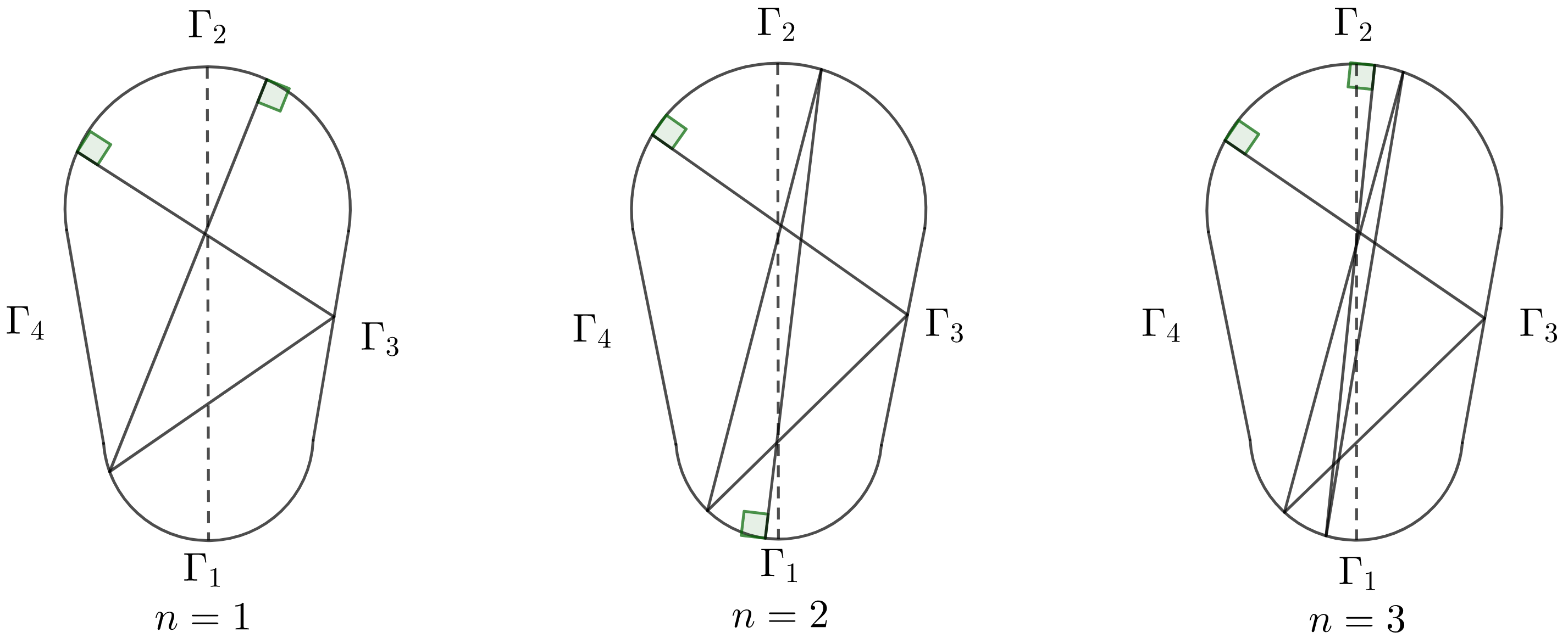
Figure 2: The palindromic orbit $\gamma_{n}$ with $n=1,2,3$

We first need to show the existence and uniqueness of such orbits.

Lemma 4.1.

For any $n\geq 1$, there exists a unique palindromic periodic orbit $\gamma_{n}$ associated with the symbolic sequence (4.1).

Proof.

Let $\widetilde{\Omega}$ be the double cover table of $\Omega$ (see Fig. 1, right), and let $\widetilde{\Gamma}_{i}$ be the new boundaries of $\widetilde{\Omega}$, which corresponds to the code $\widetilde{i}$ for $i=1,2,4$. Then $(r_{0}^{-}\overline{r}_{0}r_{0}^{+}r_{1}\dots r_{2n+1})$ forms a periodic orbit in $\Omega$ associated with (4.1), if and only if $(r_{0}r_{1}\dots r_{2n+1})$ forms a periodic orbit in $\widetilde{\Omega}$ associated with

$$(\widetilde{2}\underbrace{12\cdots 121}_{2n+1}),$$ (4.2)

where $r_{0}$ is the symmetric point of $\overline{r}_{0}$ with respect to $\Gamma_{3}$. To this end, we recall that $\widetilde{\tau}(\cdot,\cdot)$ is the free path in $\widetilde{\Omega}$, and consider the length function

$$L(r_{0},r_{1},\dots,r_{2n+1})=\sum_{k=0}^{2n+1}\widetilde{\tau}(r_{k},r_{k+1}),$$

for $(r_{0},r_{1},\dots,r_{2n+1})\in\widetilde{\Gamma}_{2}\times\left(\Gamma_{1}\times\Gamma_{2}\right)^{n}\times\Gamma_{1}$, where we set $r_{2n+2}=r_{0}$. Let $\varphi(r_{k},r_{k+1})$ (resp. $\varphi_{1}(r_{k},r_{k+1})$) be the angle formed by the vector $\overline{r_{k}r_{k+1}}$ and the inward (resp. outward) inner normal vector at $r_{k}$ (resp. at $r_{k+1}$). By (2.4),

$$\frac{\partial L}{\partial r_{k}}=\frac{\partial\widetilde{\tau}}{\partial r_{k}}(r_{k-1},r_{k})+\frac{\partial\widetilde{\tau}}{\partial r_{k}}(r_{k},r_{k+1})=\sin\varphi_{1}(r_{k-1},r_{k})-\sin\varphi(r_{k},r_{k+1}).$$

It follows that $(r_{0},r_{1},\dots,r_{2n+1})$ forms a periodic orbit, if and only if it is a critical point of $L$. Similar to the proof of Lemma 3.1, the Hessian matrix of $L$ is negative definite due to the doubly focusing mechanism. Thus, $L$ is a strictly concave function on the compact domain $\widetilde{\Gamma}_{2}\times\left(\Gamma_{1}\times\Gamma_{2}\right)^{n}\times\Gamma_{1}$, and there can be at most one critical point for $L$.

On the other hand, $L$ has a global maximum point $\widetilde{\gamma}_{n}=(r_{0},r_{1},\dots,r_{2n+1})$ which must be an interior point. Therefore, $\widetilde{\gamma}_{n}$ is the only critical point of $L$, which forms a periodic orbit in $\widetilde{\Omega}$ associated with (4.2). Noticing that

$$L(r_{0},r_{1},r_{2},\dots,r_{n+1},\dots,r_{2n},r_{2n+1})=L(r_{0},r_{2n+1},r_{2n},\dots,r_{n+1},\dots,r_{2},r_{1}),$$

we further get $r_{n+2-k}=r_{k}$ for $1\leq k\leq n$, that is, the orbit $\widetilde{\gamma}_{n}$ is palindromic. Finally, we obtain the unique periodic orbit $\gamma_{n}:=(r_{0}^{-}\overline{r}_{0}r_{0}^{+}r_{1}\dots r_{2n+1})$ in $\Omega$ associated with (4.1), where $\overline{r}_{0}$ is the symmetric point of $r_{0}$ with respect to $\Gamma_{3}$, and $r_{0}^{\pm}$ is obtained as the intersection between $\overline{r_{0}r_{1}}$ and $\Gamma_{3}$. ∎

4.2 The Homoclinic Semi-orbit $\gamma_{\infty}$

We denote the collision points of $\gamma_{n}$ by

$$y_{n}(0^{-})\mapsto x_{n}(0)\mapsto y_{n}(0)\mapsto x_{n}(1)\mapsto y_{n}(1)\mapsto\dots\mapsto x_{n}(n)\mapsto y_{n}(n)\mapsto x_{n}(n+1),$$

where

• at the initial stages corresponding to the codes $(323)$, we denote by $x_{n}(0)=(s_{n}(0),0)$ the collision point on $\Gamma_{2}$, and denote by $y_{n}(0)=(t_{n}(0),\psi_{n}(0))$ and $y_{n}(0^{-})=(t_{n}(0),-\psi_{n}(0))$ the two collision points on $\Gamma_{3}$.

• at the stage of $2n+1$ successive collisions between $\Gamma_{1}$ and $\Gamma_{2}$, we denote

  $$\text{on}\ \Gamma_{1}:\ x_{n}(k) =(s_{n}(k),\varphi_{n}(k)),\ k=1,2,\dots,n,n+1;$$

  $$\text{on}\ \Gamma_{2}:\ y_{n}(k) =(t_{n}(k),\psi_{n}(k)),\ k=1,2,\dots,n.$$

By time reversibility, we have

$$\begin{split}s_{n}(n+2-k)=s_{n}(k),\ &\ \varphi_{n}(n+2-k)=-\varphi_{n}(k),\ k=1,2,\dots,n+1,\\ t_{n}(n+1-k)=t_{n}(k),\ &\ \psi_{n}(n+1-k)=-\psi_{n}(k),\ k=1,2,\dots,n.\end{split}$$ (4.3)

In particular, $\varphi_{n}(\frac{n+2}{2})=0$ if $n$ is even, and $\psi_{n}(\frac{n+1}{2})=0$ is $n$ is odd.

We first provide some rough estimates.

Lemma 4.2.

There exists $C>0$ such that for any $n\geq 1$ and $m\geq 0$,

$$\begin{split}\|x_{n+m}(k)-x_{n}(k)\|&\leq C\Lambda^{2k-2n},\ \ \ \ \ k=0,1,\dots,n+1,\\ \|y_{n+m}(k)-y_{n}(k)\|&\leq C\Lambda^{2k-2n},\ \ \ \ \ k=0^{-},0,1,\dots,n.\end{split}$$

where the constant $\Lambda>1$ is given by (2.2), and $\|\cdot\|$ denotes the Euclidean norm in the phase space $M$.

Proof.

Recall that the billiard ball hits $\Gamma_{2}$ perpendicularly in the initial stage of $\gamma_{n}$ and $\gamma_{n+m}$, that is, $x_{n}(0)=(s_{n}(0),0)$ and $x_{n+m}(0)=(s_{n+m}(0),0)$. Let $W$ be the wave front between $s=s_{n}(0)$ and $s=s_{n+m}(0)$, associated with zero angles. Then $W$ is an unstable curve, so is its forward iterate $F^{k}(W)$ for any $k\geq 0$, unless $F^{k}(W)$ is cut by singularities, i.e., $F^{k}(W)$ hits the gluing points.

Following the trajectories of $\gamma_{n}$ and $\gamma_{n+m}$, it is not hard to see that $F^{k}(W)$ stays away from the singularities for $0\leq k\leq 2n+1$. Furthermore, the transition from $F^{k}(W)$ to $F^{k+1}(W)$ is between $\Gamma_{1}$ and $\Gamma_{2}$, for $2\leq k\leq 2n+1$, then by (2.3), we have the following estimates for the $p$-length of $F^{k}(W)$:

$$|F^{k+i}(W)|_{p}\geq\Lambda^{i}|F^{k}(W)|_{p},\ \ 2\leq k\leq k+i\leq 2n+2.$$

At Step $k=0$, $W$ goes from $\Gamma_{2}$ and hits the flat wall $\Gamma_{3}$, and then at Step $k=1$, it collides on $\Gamma_{1}$. Thus, $|F^{2}(W)|_{p}\geq\Lambda|W|_{p}$.

Note that there is $\varphi_{0}\in(0,\pi/2)$ such that $|\varphi|\leq\varphi_{0}$ for any point $z=(r,\varphi)$ lying on $\Gamma_{1}$ (resp. on $\Gamma_{2}$) satisfying the following properties:

• $F^{-1}(z)$ lies on $\Gamma_{2}$ (resp. on $\Gamma_{1}$), or $F^{-1}(z)$ lies on $\Gamma_{3}$ but $F^{-2}(z)$ lies on $\Gamma_{2}$ (resp. on $\Gamma_{1}$);

• $F(z)$ lies on $\Gamma_{2}$ (resp. on $\Gamma_{1}$), or $F(z)$ lies on $\Gamma_{3}$ but $F^{2}(z)$ lies on $\Gamma_{2}$ (resp. on $\Gamma_{1}$).

Therefore, the angle variables on all the curves $\{F^{k}(W)\}_{k\geq 0}$ have absolute value bounded by $\varphi_{0}$. Hence there is $C_{0}>0$ such that for any $k\geq 0$,

$$|F^{k}(W)|/C_{0}\leq|F^{k}(W)|_{p}\leq C_{0}|F^{k}(W)|.$$

Set $C=C_{0}^{2}{\rm diam}(M)$. Note that $x_{n}(0)$ and $x_{n+m}(0)$ are the endpoints of $W$, then

$$\|x_{n+m}(0)-x_{n}(0)\|=|W|\leq C_{0}|W|_{p}\leq C_{0}\Lambda^{-2n}|F^{2n+1}(W)|_{p} \leq C_{0}^{2}\Lambda^{-2n}|F^{2n+1}(W)|$$

$$\leq C\Lambda^{-2n}.$$

The remaining estimates in this lemma can be shown in a similar fashion, by noticing the following facts: $x_{n}(k)$ and $x_{n+m}(k)$ are endpoints of $F^{2k}(W)$ for $1\leq k\leq n+1$; $y_{n}(k)$ and $y_{n+m}(k)$ are endpoints of $F^{2k+1}(W)$ for $0\leq k\leq n$. ∎

By Lemma 4.2, we define

$$\begin{split}x_{\infty}(k)&=\lim_{n\to\infty}x_{n}(k),\ k=0,1,2,\dots;\\ y_{\infty}(k)&=\lim_{n\to\infty}y_{n}(k),\ k=0^{-},0,1,2,\dots.\end{split}$$ (4.4)

Then we obtain a semi-orbit

$$\gamma_{\infty}:=(y_{\infty}(0^{-})\ x_{\infty}(0)\ y_{\infty}(0)\ x_{\infty}(1)\ y_{\infty}(1)\dots\ x_{\infty}(k)\ y_{\infty}(k)\dots),$$

which corresponds to the symbolic code $(323121212\cdots)$. The following lemma shows that $\gamma_{\infty}$ is a homoclinic semi-orbit of the period two orbit $\gamma^{*}=\overline{xy}$.

Lemma 4.3.

$\lim\limits_{k\to\infty}x_{\infty}(k)=x$, and $\lim\limits_{k\to\infty}y_{\infty}(k)=y$.

Proof.

For any $k\geq 1$, by Lemma 4.2, we take $n=2k-1$ and let $m\to\infty$, then

$$\|x_{\infty}(k)-x_{2k-1}(k)\|\leq C\Lambda^{-2k+2}.$$

On the other hand, the trajectory $\gamma_{2k-1}$ hits perpendicularly at $\Gamma_{1}$ at the $k$-th step, i.e., $x_{2k-1}(k)=(s_{2k-1}(k),0)$. Also, we note that the period two point on $\Gamma_{1}$ is given by $x=(0,0)$. Let $W$ be the wave front between $s=s_{2k-1}(k)$ and $s=0$, associated with zero angles. Then $W$ is an unstable curve, and so is $F^{\ell}(W)$ for any $0\leq\ell\leq k-1$ since $F^{\ell}(W)$ does not hit the gluing points. Therefore, $|F^{k-1}(W)|_{p}\geq\Lambda^{k-1}|W|_{p}$. Similar to the proof of Lemma 4.2, we obtain

$$\|x_{2k-1}(k)-x\|=|s_{2k-1}(k)-0|\leq C\Lambda^{-k+1},$$

and thus, $\|x_{\infty}(k)-x\|\leq 2C\Lambda^{-k+1}$, which implies that $\lim\limits_{k\to\infty}x_{\infty}(k)=x$. The other limiting result $\lim\limits_{k\to\infty}y_{\infty}(k)=y$ can be proven in a similar way. ∎

We denote the coordinates of $\gamma_{\infty}$ as

$$x_{\infty}(k) =(s_{\infty}(k),\varphi_{\infty}(k)),\ k=0,1,2,\dots;$$

$$y_{\infty}(k) =(t_{\infty}(k),\psi_{\infty}(k)),\ k=0,1,2,\dots,$$

and $y_{\infty}(0^{-})=(t_{\infty}(0),-\psi_{\infty}(0))$. Note that $\varphi_{\infty}(0)=\lim\limits_{n\to\infty}\varphi_{n}(0)=0$.

4.3 The Convergence of $\gamma_{\infty}$ to $\gamma^{*}$ and the Shadowing of $\gamma_{n}$ along $\gamma_{\infty}$

Recall that $\lambda>1$ is the leading eigenvalue of $DF^{2}$ along the period two orbit $\gamma^{*}=\overline{xy}$. The next lemma provides finer estimates of the asymptotic convergence of the homoclinic orbit $\gamma_{\infty}$ to the period two orbit $\gamma^{*}$, as well as the shadowing estimates of $\gamma_{n}$ along $\gamma_{\infty}$.

Lemma 4.4.

• The following estimates hold for the homoclinic orbit $\gamma_{\infty}$:

  $$\begin{split}x_{\infty}(k)=\lambda^{-k}(C_{s},C_{\varphi})+\mathcal{O}(\lambda^{-1.5k}),&\ \ k=0,1,2,\dots,\\ y_{\infty}(k)=\lambda^{-k}(C_{t},C_{\psi})+\mathcal{O}(\lambda^{-1.5k}),&\ \ k=0,1,2,\dots,\end{split}$$ (4.5)

  where the constants $C_{s},C_{\varphi},C_{t}$ and $C_{\psi}$ satisfy the following relation:

  $$\dfrac{C_{\varphi}}{C_{s}}=\frac{\lambda^{-1}-\lambda}{4a_{2}\tau^{*}},\ \ \dfrac{C_{\psi}}{C_{t}}=\frac{\lambda^{-1}-\lambda}{4a_{1}\tau^{*}},\ \ \dfrac{C_{t}}{C_{s}}=-\frac{1+\lambda^{-1}}{2a_{2}}=-\frac{2a_{1}}{1+\lambda}.$$ (4.6)

• The following estimates hold for the palindromic orbit $\gamma_{n}$:

  $$\begin{split}x_{n}(k)-x_{\infty}(k)=\lambda^{k-n}(C_{s,k},C_{\varphi,k})+\mathcal{O}(\lambda^{0.5k-n}),&\ \ k=0,1,\dots,\left\lfloor{\frac{n}{2}}\right\rfloor+1,\\ y_{n}(k)-y_{\infty}(k)=\lambda^{k-n}(C_{t,k},C_{\psi,k})+\mathcal{O}(\lambda^{0.5k-n}),&\ \ k=0,1,\dots,\left\lfloor{\frac{n}{2}}\right\rfloor.\end{split}$$ (4.7)

  Here the constants $C_{s,k},C_{\varphi,k},C_{t,k}$ and $C_{\psi,k}$ are given by

  $$\begin{split}C_{s,k}=C_{s}\,\lambda^{-2}\,(\lambda^{-2k}+1),\ \ &\ \ C_{\varphi,k}=C_{\varphi}\,\lambda^{-2}\,(\lambda^{-2k}-1),\\ C_{t,k}=C_{t}\,\lambda^{-1}\,(\lambda^{-2k}+1),\ \ &\ \ C_{\psi,k}=C_{\psi}\,\lambda^{-1}\,(\lambda^{-2k}-1).\end{split}$$ (4.8)

Proof.

Let $U_{1}$ and $U_{2}$ be the neighborhood of $x$ and $y$ respectively, which are given by Lemma 3.2. Choose an integer $k_{0}>0$ such that $x_{n}(k)\in U_{1}$ for all $k\in[k_{0},n+2-k_{0}]$ and $y_{n}(k)$ for all $k\in[k_{0},n+1-k_{0}]$. We apply the coordinate change given by (3.9), that is, $x_{n}(k)$ and $y_{n}(k)$ are represented by $(\xi_{n}(k),\eta_{n}(k))$ and $(\zeta_{n}(k),\iota_{n}(k))$ respectively, for $k\geq k_{0}$. Set

$$\xi_{n}=\lambda^{-k_{0}}\xi_{n}(k_{0}),\ \ \eta_{n}=\lambda^{k_{0}}\eta_{n}(k_{0}),\ \ \zeta_{n}=\lambda^{-k_{0}}\zeta_{n}(k_{0}),\ \ \iota_{n}=\lambda^{k_{0}}\iota_{n}(k_{0}).$$ (4.9)

Then (3.12) implies that

$$\xi_{n}(k)=\lambda^{k}\xi_{n},\ \ \eta_{n}(k)=\lambda^{-k}\eta_{n},\ \ \zeta_{n}(k)=\lambda^{k}\zeta_{n},\ \ \iota_{n}(k)=\lambda^{-k}\iota_{n}.$$ (4.10)

These formulas also hold for $x_{n}(k)$ with $k\in[0,k_{0})\cup(n+2-k_{0},n+1]$ and for $y_{n}(k)$ with $k\in[0,k_{0})\cup(n+1-k_{0},n]$, by suitably extending $\Psi_{1}$ and $\Psi_{2}$ along a neighborhood of the separatrices of $\gamma^{*}$. In particular, we denote

$$\xi_{n}(0)=\xi_{n},\ \ \eta_{n}(0)=\eta_{n},\ \ \zeta_{n}(0)=\zeta_{n},\ \ \iota_{n}(0)=\iota_{n}.$$

(a) We first show the estimates along the homoclinic orbit $\gamma_{\infty}$. The coordinates of $x_{\infty}(k)$ are denoted by $(\xi_{\infty}(k),\eta_{\infty}(k))$ for $k=0,1,2,\dots$, and the coordinates of $y_{\infty}(k)$ are denoted by $(\zeta_{\infty}(k),\iota_{\infty}(k))$ for $k=0^{-},0,1,2,\dots$. By (4.4) and (4.9), the following limits exist:

$$\xi_{\infty}=\lim\limits_{n\to\infty}\xi_{n},\ \ \eta_{\infty}=\lim\limits_{n\to\infty}\eta_{n},\ \ \zeta_{\infty}=\lim\limits_{n\to\infty}\zeta_{n},\ \ \iota_{\infty}=\lim\limits_{n\to\infty}\iota_{n}.$$

By passing $n\to\infty$ in (4.10), we have for any $k\geq 0$,

$$\xi_{\infty}(k)=\lambda^{k}\xi_{\infty},\ \ \eta_{\infty}(k)=\lambda^{-k}\eta_{\infty},\ \ \zeta_{\infty}(k)=\lambda^{k}\zeta_{\infty},\ \ \iota_{\infty}(k)=\lambda^{-k}\iota_{\infty}.$$

It is clear that $\lambda^{-k_{0}}x_{\infty}(k_{0})=(\xi_{\infty},\eta_{\infty})$ and $\lambda^{-k_{0}}y_{\infty}(k_{0})=(\zeta_{\infty},\iota_{\infty})$.

Note that $\lim\limits_{k\to\infty}x_{\infty}(k)=x$ implies that $x_{\infty}(k)$ lies on the local stable manifold $W^{s}(x)=\{(\xi,\eta):\ \xi=0\}$, and thus, $\xi_{\infty}(k)=\xi_{\infty}=0$ for all $k\geq 0$. Hence

$$x_{\infty}(k)=\begin{pmatrix}s_{\infty}(k)\\ \varphi_{\infty}(k)\end{pmatrix}=\Psi_{1}\circ\Theta_{1}\begin{pmatrix}\xi_{\infty}(k)\\ \eta_{\infty}(k)\end{pmatrix} =\Psi_{1}\circ\begin{pmatrix}\ \ \cos\theta_{1}&\cos\theta_{1}\\ -\sin\theta_{1}&\sin\theta_{1}\end{pmatrix}\begin{pmatrix}0\\ \lambda^{-k}\eta_{\infty}\end{pmatrix}$$

$$=\Psi_{1}\left(\lambda^{-k}\eta_{\infty}\begin{pmatrix}\cos\theta_{1}\\ \sin\theta_{1}\end{pmatrix}\right)-\Psi_{1}(0,0)$$

$$=\lambda^{-k}\begin{pmatrix}C_{s}\\ C_{\varphi}\end{pmatrix}+\mathcal{O}(\lambda^{-1.5k}),$$

where we set $C_{s}:=\eta_{\infty}\cos\theta_{1}$ and $C_{\varphi}:=\eta_{\infty}\sin\theta_{1}$. Similarly, since $y_{\infty}(k)$ lies on the local stable manifold $W^{s}(y)=\{(\zeta,\iota):\ \zeta=0\}$, we obtain that $\zeta(k)=\zeta_{\infty}=0$ for any $k\geq 0$, and thus,

$$y_{\infty}(k)=\begin{pmatrix}t_{\infty}(k)\\ \psi_{\infty}(k)\end{pmatrix}=\lambda^{-k}\begin{pmatrix}C_{t}\\ C_{\psi}\end{pmatrix}+\mathcal{O}(\lambda^{-1.5k}),$$

where we set $C_{t}:=\iota_{\infty}\cos\theta_{2}$ and $C_{\psi}:=\iota_{\infty}\sin\theta_{2}$.

The first two relations in (4.6), that is, $C_{\varphi}/C_{s}=\tan\theta_{1}$ and $C_{\psi}/C_{t}=\tan\theta_{2}$, directly follows from (3.5) and (3.6). Moreover, by (3.10), we have $\iota_{\infty}=\lambda_{1,s}\eta_{\infty}$, and hence the third relation in (4.6), that is, $C_{t}/C_{s}=\lambda_{1,s}\cos\theta_{2}/\cos\theta_{1}$, directly follows from (3.7) and (3.3).

(b) We now show the estimates for the palindromic orbits $\gamma_{n}$. Note that there are involutions given by $\mathcal{I}_{1}:(s,\varphi)\mapsto(s,-\varphi)$ and $\mathcal{I}_{2}:(t,\psi)\mapsto(t,-\psi)$. Let $\mathcal{J}_{1}(\xi,\eta):=\Theta_{1}^{-1}\circ\Psi_{1}^{-1}\circ\mathcal{I}_{1}\circ\Psi_{1}\circ\Theta_{1}(\xi,\eta)$, then $\mathcal{J}_{1}(0,0)=(0,0)$ and

$$\mathcal{J}_{1}\begin{pmatrix}\xi\\ \eta\end{pmatrix} =\begin{pmatrix}\ \ \cos\theta_{1}&\cos\theta_{1}\\ -\sin\theta_{1}&\sin\theta_{1}\end{pmatrix}^{-1}\begin{pmatrix}1&0\\ 0&-1\end{pmatrix}\begin{pmatrix}\ \ \cos\theta_{1}&\cos\theta_{1}\\ -\sin\theta_{1}&\sin\theta_{1}\end{pmatrix}\begin{pmatrix}\xi\\ \eta\end{pmatrix}+\mathcal{O}\left((|\xi|^{2}+|\eta|^{2})^{\frac{3}{2}}\right)$$

$$=\begin{pmatrix}\eta\\ \xi\end{pmatrix}+\mathcal{O}\left(\max\{|\xi|,|\eta|\}^{\frac{3}{2}}\right),$$

and $$\ \ \mathcal{J}_{1}\begin{pmatrix}\xi\\ \eta\end{pmatrix}-\mathcal{J}_{1}\begin{pmatrix}\xi^{\prime}\\ \eta^{\prime}\end{pmatrix}=\begin{pmatrix}\eta-\eta^{\prime}\\ \xi-\xi^{\prime}\end{pmatrix}+\mathcal{O}\left(\max\{|\xi-\xi^{\prime}|,|\eta-\eta^{\prime}|\}^{\frac{3}{2}}\right).$$

We have similar properties for $\mathcal{J}_{2}(\zeta,\iota):=\Theta_{2}^{-1}\circ\Psi_{2}^{-1}\circ\mathcal{I}_{2}\circ\Psi_{2}\circ\Theta_{2}(\zeta,\iota)$.

By time reversibility (4.3), $(s_{n}(n+2-k),\varphi_{n}(n+2-k)=\mathcal{I}_{1}(s_{n}(k),\varphi_{n}(k))$ for any $1\leq k\leq[\tfrac{n}{2}]+1$, and hence correspondingly,

$$(\lambda^{n+2-k}\xi_{n},\lambda^{k-n-2}\eta_{n}) =(\xi_{n}(n+2-k),\eta_{n}(n+2-k))$$

$$=\mathcal{J}_{1}(\xi_{n}(k),\eta_{n}(k))$$

$$=\mathcal{J}_{1}(\lambda^{k}\xi_{n},\lambda^{-k}\eta_{n})$$

$$=(\lambda^{-k}\eta_{n},\lambda^{k}\xi_{n})+\mathcal{O}\left(\max\{\lambda^{1.5k}|\xi_{n}|^{1.5},\ \lambda^{-1.5k}|\eta_{n}|^{1.5}\}\right).$$

It follows that $\xi_{n}=\mathcal{O}(\lambda^{-n})$ by taking $k=1$, and further, $\xi_{n}=\eta_{n}\lambda^{-n-2}+\mathcal{O}\left(\lambda^{-1.25n}\right)$ by taking $k=\lfloor(n+2)/2\rfloor$.

On the other hand, recall that $x_{n}(0)=(s_{n}(0),0)$ and $x_{\infty}(0)=(s_{\infty}(0),0)$, which are unchanged under the involution $\mathcal{I}_{1}$. Correspondingly, $\mathcal{J}_{1}(\xi_{n},\eta_{n})=(\xi_{n},\eta_{n})$ and $\mathcal{J}_{1}(0,\eta_{\infty})=(0,\eta_{\infty})$. Then

$$(\xi_{n},\eta_{n}-\eta_{\infty})=\mathcal{J}_{1}(\xi_{n},\eta_{n})-\mathcal{J}_{1}(0,\eta_{\infty})=(\eta_{n}-\eta_{\infty},\xi_{n})+\mathcal{O}\left(\max\left\{|\xi_{n}|,|\eta_{n}-\eta_{\infty}|\right\}^{\frac{3}{2}}\right),$$

which implies that

$$\eta_{n}-\eta_{\infty}=\xi_{n}+\mathcal{O}(\lambda^{-1.5n})=\eta_{n}\lambda^{-n-2}+\mathcal{O}(\lambda^{-1.25n}).$$

Thus, $\eta_{n}-\eta_{\infty}=\eta_{\infty}\lambda^{-n-2}+\mathcal{O}(\lambda^{-1.25n})$, and $\xi_{n}=\eta_{\infty}\lambda^{-n-2}+\mathcal{O}(\lambda^{-1.25n})$. Hence for any $0\leq k\leq\lfloor\frac{n}{2}\rfloor+1$,

$$x_{n}(k)-x_{\infty}(k) =\begin{pmatrix}s_{n}(k)\\ \varphi_{n}(k)\end{pmatrix}-\begin{pmatrix}s_{\infty}(k)\\ \varphi_{\infty}(k)\end{pmatrix}$$

$$=\Psi_{1}\circ\Theta_{1}\begin{pmatrix}\xi_{n}(k)\\ \eta_{n}(k)\end{pmatrix}-\Psi_{1}\circ\Theta_{1}\begin{pmatrix}\xi_{\infty}(k)\\ \eta_{\infty}(k)\end{pmatrix}$$

$$=\begin{pmatrix}\ \ \cos\theta_{1}&\cos\theta_{1}\\ -\sin\theta_{1}&\sin\theta_{1}\end{pmatrix}\begin{pmatrix}\lambda^{k}\xi_{n}\\ \lambda^{-k}(\eta_{n}-\eta_{\infty})\end{pmatrix}+\mathcal{O}\left(\max\left\{\lambda^{1.5(k-n)},\lambda^{-1.5k-n}\right\}\right)$$

$$=\lambda^{k-n-2}\begin{pmatrix}\eta_{\infty}\cos\theta_{1}(\lambda^{-2k}+1)\\ \eta_{\infty}\sin\theta_{1}(\lambda^{-2k}-1)\end{pmatrix}+\mathcal{O}\left(\lambda^{0.5k-n}\right)$$

$$=\lambda^{k-n}\begin{pmatrix}C_{s}\lambda^{-2}(\lambda^{-2k}+1)\\ C_{\varphi}\lambda^{-2}(\lambda^{-2k}-1)\end{pmatrix}+\mathcal{O}\left(\lambda^{0.5k-n}\right).$$

The estimates of $y_{n}(k)-y_{\infty}(k)$ can be shown in a similar fashion. The proof of this lemma is complete. ∎

Remark 4.5.

We make some comments on the consequences of (4.7).

• When $k\approx\frac{n}{2}$, i.e., $\frac{n}{2}-m\leq k\leq\frac{n}{2}$ for some fixed $m\in{\mathbb{N}}$, we have

  $$\begin{split}x_{n}(k)=\left(C_{s}\left(\lambda^{-k}+\lambda^{k-n-2}\right),C_{\varphi}\left(\lambda^{-k}-\lambda^{k-n-2}\right)\right)+\mathcal{O}(\lambda^{-0.75n}),\\ y_{n}(k)=\left(C_{t}\left(\lambda^{-k}+\lambda^{k-n-1}\right),C_{\psi}\left(\lambda^{-k}-\lambda^{k-n-1}\right)\right)+\mathcal{O}(\lambda^{-0.75n}).\end{split}$$ (4.11)

  From the proof of (4.7), it is not hard to see that the above estimates hold for $\frac{n}{2}\leq k\leq\frac{n}{2}+m$ as well, after possibly enlarging the constants in $\mathcal{O}(\cdot)$.

• When $\varepsilon n\leq k\leq\frac{n}{2}$ for some $\varepsilon\in(0,\frac{1}{2})$, we have

  $$x_{n}(k)-x_{\infty}(k)=\lambda^{k-n}\left[(C_{s,k},C_{\varphi,k})+o(1)\right],\ \ \text{as}\ n\to\infty.$$ (4.12)

  It immediately follows that $x_{n}(k)$ asymptotically lies on a straight line which goes through $x_{\infty}(k)$ and has direction vector $(C_{s,k},C_{\varphi,k})$ when $n\to\infty$ and $k/n\geq\varepsilon$. Similar formulas hold for $y_{n}(k)-y_{\infty}(k)$.

  However, when $k$ is a finite value, we can only conclude that $x_{n}(k)-x_{\infty}(k)=\mathcal{O}(\lambda^{k-n})$. In the following lemma, We shall see that (4.12) still holds for all $k\in[0,\lfloor n/2\rfloor+1]$, though the new coefficients are in lack of precise formulas.

Lemma 4.6.

The following estimates hold for the palindromic orbit $\gamma_{n}$: as $n\to\infty$,

$$\begin{split}x_{n}(k)-x_{\infty}(k)=\lambda^{k-n}\left[v_{\infty}(2k)+o(1)\right],\ \ \ \ \ \ &\ \ k=0,1,\dots,\left\lfloor{\frac{n}{2}}\right\rfloor+1,\\ y_{n}(k)-y_{\infty}(k)=\lambda^{k-n}\left[v_{\infty}(2k+1)+o(1)\right],\ &\ \ k=0,1,\dots,\left\lfloor{\frac{n}{2}}\right\rfloor,\end{split}$$ (4.13)

where the vectors $v_{\infty}(m)\in{\mathbb{R}}^{2}$, $m=0^{\pm},0,1,2,\dots$, has uniformly bounded magnitudes.

Proof.

Recall that $x_{n}(0)=(s_{n}(0),0)$ and $x_{\infty}(0)=(s_{\infty}(0),0)$, which are all stay uniform distance away from the singular set (i.e. corner points). It suffices to show that there is $s_{\infty}\in{\mathbb{R}}$ such that

$$s_{n}(0)-s_{\infty}(0)=\lambda^{-n}\left[s_{\infty}+o(1)\right].$$ (4.14)

Indeed, if (4.14) holds, then by setting $v_{\infty}(0)=(s_{\infty},0)\in{\mathbb{R}}^{2}$ we have

$$x_{n}(0)-x_{\infty}(0)=(s_{n}(0)-s_{\infty}(0),0)=\lambda^{-n}\left[v_{\infty}(0)+o(1)\right].$$

Furthermore, for any $1\leq k\leq\left\lfloor{\frac{n}{2}}\right\rfloor+1$, there exists $C_{k}^{\prime}>0$ such that

$$x_{n}(k)-x_{\infty}(k) = F^{2k}(x_{n}(0))-F^{2k}(x_{\infty}(0))$$

$$= D_{x_{\infty}(0)}F^{2k}(x_{n}(0)-x_{\infty}(0))+C_{k}^{\prime}\left(x_{n}(0)-x_{\infty}(0)\right)^{2}$$

$$= \lambda^{k-n}\cdot\lambda^{-k}D_{x_{\infty}(0)}F^{2k}v_{\infty}(0)+o(\lambda^{-n})$$

$$= \lambda^{k-n}\left[v_{\infty}(2k)+o(1)\right],$$

where in the last identity we set $v_{\infty}(2k):=\lambda^{-k}D_{x_{\infty}(0)}F^{2k}v_{\infty}(0)$, and $D_{x_{\infty}(0)}F^{2k}$ is the differential of $F^{2k}$ evaluated at $x_{\infty}(0)$. Similarly, for any $1\leq k\leq\left\lfloor{\frac{n}{2}}\right\rfloor$, we set $v_{\infty}(2k+1):=\lambda^{-k}D_{x_{\infty}(0)}F^{2k+1}v_{\infty}(0)$, then

$$y_{n}(k)-y_{\infty}(k)=F^{2k+1}(x_{n}(0))-F^{2k+1}(x_{\infty}(0))=\lambda^{k-n}\left[v_{\infty}(2k+1)+o(1)\right].$$

In the rest of the proof, we concentrate on how to obtain (4.14). The proof is based on a geometric arguments by considering the growth of a special dispersing wave front. To be precise, let $W$ be the wave front between $s=s_{n}(0)$ and $s=s_{\infty}(0)$, associated with zero angles. Without loss of generality, we may assume $s_{n}(0)>s_{\infty}(0)$, then

$$W=\left\{x(s)=s(1,0)\left|\ s_{\infty}(0)\leq s\leq s_{n}(0)\right.\right\}.$$

It is clear that $W$ is an unstable curve connecting $x_{n}(0)$ and $x_{\infty}(0)$, such that $F^{2m}(W)$ is an unstable curve connecting $x_{n}(m)$ and $x_{\infty}(m)$ for any $1\leq m\leq n$. Moreover,

$$\left|F^{2m}(W)\right|=\int_{s_{\infty}(0)}^{s_{n}(0)}\left\|D_{x(s)}F^{2m}(1,0)\right\|ds.$$

On the one hand, the semi-orbit $\gamma_{\infty}$ is homoclinic to the period two orbit $\gamma^{*}$ whose Lyapunov exponent along the unstable direction is equal to $\frac{1}{2}\log\lambda$, and the vector $(1,0)$ is in the unstable cone $\mathcal{C}^{u}(x_{\infty}(0))$, there is a constant $C_{\infty}>0$ such that

$$\left\|D_{x_{\infty}(0)}F^{2m}(1,0)\right\|=\lambda^{m}C_{\infty}+o(1),\ \ \text{as}\ m\to\infty.$$

On the other hand, by Lemma 4.5, we have $x_{n}(m)-x_{\infty}(m)=\mathcal{O}(\lambda^{m-n})$ for any $0\leq m\leq\lfloor\frac{n}{2}\rfloor+1$. Furthermore, recall that $\mathcal{I}_{1}$ is the involution given by $\mathcal{I}_{1}(s,\varphi)=(s,-\varphi)$, and the time reversibility (4.3) implies that $x_{n}(n+2-m)=\mathcal{I}_{1}x_{n}(m)$. Hence $x_{n}(n+2-m)-\mathcal{I}_{1}x_{\infty}(m)=\mathcal{O}(\lambda^{m-n})$ for any $1\leq m\leq\lfloor\frac{n}{2}\rfloor+1$. Note that the reflected homoclinic semi-orbit $\mathcal{I}\gamma_{\infty}$ have Lyapunov exponent $\frac{1}{2}\log\lambda$ along the unstable direction as well. Since the curvature of unstable curves $\{F^{2m}(W)\}_{0\leq m\leq n}$ are uniformly bounded, we have for any $m=1,2,\dots,\lfloor\frac{n}{2}\rfloor+1$ and for any $s\in[s_{\infty}(0),s_{n}(0)]$,

$$F^{2m}(x(s))-x_{\infty}(m)=\mathcal{O}(\lambda^{m-n})\ \ \text{and}\ \ F^{2n-2m}(x(s))-\mathcal{I}_{1}x_{\infty}(m)=\mathcal{O}(\lambda^{m-n}).$$

Therefore, we have

$$\left\|D_{x(s)}F^{2n}(1,0)\right\|$$

$$= \left\|\prod^{1}_{m=n+1-\lfloor\frac{n}{2}\rfloor}D_{F^{2(n-m)}(x(t))}F^{2}\prod_{m=0}^{\lfloor\frac{n}{2}\rfloor}D_{F^{2m}(x(t))}F^{2}\cdot(1,0)\right\|$$

$$= \left\|\prod^{1}_{m=n+1-\lfloor n/2\rfloor}\left(D_{\mathcal{I}_{1}x_{\infty}(m)}F^{2}+\mathcal{O}(\lambda^{m-n})\right)\prod_{m=0}^{\lfloor\frac{n}{2}\rfloor}\left(D_{x_{\infty}(m)}F^{2}+\mathcal{O}(\lambda^{m-n})\right)\cdot(1,0)\right\|$$

$$= \lambda^{n}(C_{\infty}+o(1)),$$

and hence

$$\left|F^{2n}W\right|=\int_{s_{\infty}(0)}^{s_{n}(0)}\left\|D_{x(t)}F^{2n}(1,0)\right\|ds=\lambda^{n}(C_{\infty}+o(1))(s_{n}(0)-s_{\infty}(0)).$$

On the other hand, since $\lim\limits_{n\to\infty}x_{\infty}(n)=x$ and $\lim\limits_{n\to\infty}x_{n}(n)=\mathcal{I}_{1}x_{\infty}(2)$, then $F^{2n}(W)$ converges to the unstable manifold $W^{\prime}$ which connects $x$ and $\mathcal{I}_{1}x_{\infty}(2)$, and hence $\left|F^{2n}W\right|=|W^{\prime}|+o(1)$ as $n\to\infty$. Therefore, $s_{n}(0)-s_{\infty}(0)=\lambda^{-n}\left[s_{\infty}+o(1)\right]$ if we set $s_{\infty}=|W^{\prime}|/C_{\infty}$. The proof of this lemma is complete. ∎

5 The Linearized Isospectral Functionals

To prove Squash Rigidity Theorem, we introduce the linearized isospectral functionals corresponding to periodic orbits of the Bunimovich squash-type stadia.

5.1 Normalization, Parametrization and Deformation

Let $\Omega$ be a Bunimovich squash-type stadium in $\mathcal{M}^{m}_{ss}$, where $m\geq 3$. By Lemma 3.1, there is a unique maximal period two orbit $\gamma^{*}=\overline{AB}$ for $\Omega$. Without loss of generality, we may assume that $A$ is the origin of ${\mathbb{R}}^{2}$, and $B$ lies on the positive horizontal semiaxis of ${\mathbb{R}}^{2}$.

Let $\left\{\widehat{\Omega}_{\mu}\right\}_{|\mu|\leq 1}$ be a $C^{1}$ one-parameter family in $\mathcal{M}^{m}_{ss}$ such that $\widehat{\Omega}_{0}=\Omega$. That is, each Bunimovich squash-type stadia $\widehat{\Omega}_{\mu}$ satisfies Assumptions $\mathrm{(I_{ss})(II)(III_{ss})}$ and the convex arcs $\Gamma_{1}$ and $\Gamma_{2}$ are $C^{m}$ smooth. We would like to normalize the position of this family as follows. Lemma 3.1 shows that $\widehat{\Omega}_{\mu}$ has a unique maximal period two orbit

$$\widehat{\gamma}^{*}(\mu)=\overline{\widehat{A}(\mu)\widehat{B}(\mu)}$$

for any $\mu\in[-1,1]$. Then there is a unique orientation-preserving planar isometry $\mathcal{T}_{\mu}$ such that $\mathcal{T}_{\mu}\left(\widehat{A}(\mu)\right)=A$, $B(\mu):=\mathcal{T}_{\mu}\left(\widehat{B}(\mu)\right)$ lies on the positive horizontal semiaxis of ${\mathbb{R}}^{2}$, and $\mathcal{T}_{\mu}\left(W(\mu)\right)$ lies on positive vertical semiaxis, where $W(\mu)$ be the vector perpendicular to the vector $\overrightarrow{\widehat{A}(\mu)\widehat{B}(\mu)}$ in the counter-clockwise direction. It is easy to see from the proof of Lemma 3.1 that the dependence $\mu\mapsto\left(\widehat{A}(\mu),\widehat{B}(\mu)\right)$ is $C^{1}$ smooth, and so is the mapping $\mu\mapsto\mathcal{T}_{\mu}$ in the space of planar isometries, i.e., if we $\mathcal{T}_{\mu}(v)=E(\mu)v+F(\mu)$ for any $v\in{\mathbb{R}}^{2}$, where $E(\mu)\in\mathrm{SO}(2,{\mathbb{R}})$ and $F(\mu)\in{\mathbb{R}}^{2}$, then the mappings $\mu\mapsto E(\mu)$ and $\mu\mapsto F(\mu)$ are both $C^{1}$ smooth. We then denote

$$\Omega_{\mu}=\mathcal{T}_{\mu}\widehat{\Omega}_{\mu},\ \ \text{for}\ \ \mu\in[-1,1],$$

and call $\left\{\Omega_{\mu}\right\}_{|\mu|\leq 1}$ the normalized family of the original family $\left\{\widehat{\Omega}_{\mu}\right\}_{|\mu|\leq 1}$. Note that $\Omega_{0}=\Omega$ since $\mathcal{T}_{0}=\mathrm{Id}_{{\mathbb{R}}^{2}}$. Also, the unique maximal period two orbit of $\Omega_{\mu}$ is given by $\gamma^{*}(\mu)=\overline{AB(\mu)}$. It is clear that the normalized family $\left\{\Omega_{\mu}\right\}_{|\mu|\leq 1}$ is $C^{1}$ smooth with respect to the parameter $\mu$.

Let us now parametrize the $C^{1}$ one-parameter normalized family $\left\{\Omega_{\mu}\right\}_{|\mu|\leq 1}$ of the Bunimovich squash-type stadia such that $\Omega_{0}=\Omega$. We denote

$$\partial\Omega_{\mu}=\Gamma_{1}(\mu)\cup\Gamma_{3}(\mu)\cup\Gamma_{2}(\mu)\cup\Gamma_{4}(\mu),$$

where $\Gamma_{1}(\mu)$ and $\Gamma_{2}(\mu)$ are the two convex arcs and $\Gamma_{3}(\mu)$ and $\Gamma_{4}(\mu)$ are flat boundaries. We may choose a parametrization $\Phi:[-1,1]\times J\to{\mathbb{R}}^{2}$, where the interval $J$ is a union of four consecutive sub-intervals, i.e., $J=J_{1}\cup J_{3}\cup J_{2}\cup J_{4}$, such that

• For any $\mu\in[-1,1]$ and $i=1,2,3,4$, we have $\Phi(\mu,J_{i})=\Gamma_{i}(\mu)$;

• The mapping $\mu\mapsto\Phi(\mu,\cdot)$ is $C^{1}$ smooth;

• Set $\Phi_{i}=\Phi|_{J_{i}}$ for $i=1,2$. For any fixed $\mu\in[-1,1]$, the map $r\mapsto\Phi_{i}(\mu,r)$ is $C^{m}$ smooth.

We further define the deformation function $\mathbf{n}:[-1,1]\times J\to{\mathbb{R}}$ of the normalized family $\left\{\Omega_{\mu}\right\}_{|\mu|\leq 1}$ by

$$\mathbf{n}(\mu,r)=\mathbf{n}_{\Phi}(\mu,r):=\langle\partial_{\mu}\Phi(\mu,r),\ N(\mu,r)\rangle,$$ (5.1)

where $\langle\cdot,\cdot\rangle$ is the standard scalar product in ${\mathbb{R}}^{2}$ and $N(\mu,r)$ is the out-going unit normal vector to $\partial\Omega_{\mu}$ at the point $\Phi(\mu,r)$. It is obvious that $\mathbf{n}(\mu,r)$ is continuous in $\mu$. Moreover, for any $\mu\in[-1,1]$, the function $r\mapsto\mathbf{n}(\mu,r)$ is $C^{m}$ smooth on $J_{1}\cup J_{2}$.

Remark 5.1.

There are certainly many different choices of the parametrization that obey the above rules (1)-(3). Different parametrization $\Phi$ would surely give different deformation function $\mathbf{n}_{\Phi}$. Nevertheless, we shall only focus on the vanishing property of the deformation function, which does not depend on the parametrization at all. More precisely, let $\Phi$ and $\Phi^{\prime}$ be two parametrizations with domain interval

$$J=J_{1}\,\cup\,J_{3}\,\cup\,J_{2}\,\cup J_{4}\qquad\text{ and }\qquad J^{\prime}=J_{1}^{\prime}\,\cup J_{3}^{\prime}\,\cup J_{2}^{\prime}\,\cup\,J_{4}^{\prime},$$

respectively, by Lemma 3.3 in [9], we have $n_{\Phi}|_{J_{i}}\equiv 0$ if and only if $n_{\Phi^{\prime}}|_{J_{i}^{\prime}}\equiv 0$ for any $i=1,2,3,4$.

In the rest of the paper, we shall simply denote the deformation function by $\mathbf{n}(\mu,r)$ if the parametrization $\Phi$ is clear. To prove the Squash Rigidity Theorem, the following lemma asserts that we only need to show the vanishing of $\mathbf{n}$ on $J_{1}\cup J_{2}$.

Lemma 5.2.

If $\mathbf{n}(\mu,\cdot)\equiv 0$ on $J_{1}\cup J_{2}$ for any $\mu\in[-1,1]$, then the normalized family $\left\{\Omega_{\mu}\right\}_{|\mu|\leq 1}$ is constant, and, thus, the original family $\left\{\widehat{\Omega}_{\mu}\right\}_{|\mu|\leq 1}$ is isometric.

Proof.

By the definition of the deformation function, the condition $\mathbf{n}(\mu,\cdot)\equiv 0$ on $J_{i}$, $i=1,2$, implies that all the arcs $\Gamma_{i}(\mu)$ should lie on a common longest arc $\Gamma^{0}_{i}$. It is obvious that $\Gamma^{0}_{i}$ is a strictly convex curve. We show that in fact $\Gamma_{i}(\mu)=\Gamma^{0}_{i}$ for all $\mu\in[-1,1]$ as follows. Let $P_{14}^{0}$ be the left-top point of $\Gamma_{1}^{0}$, by compactness, there is $\mu_{0}\in[-1,1]$ such that $P_{14}(\mu_{0})=P_{14}^{0}$, where $P_{14}(\mu)$ denotes the joint point of $\Gamma_{1}(\mu)$ and $\Gamma_{4}(\mu)$. We claim that $P_{14}(\mu)=P_{14}^{0}$ for all $\mu\in[-1,1]$. Otherwise, we suppose that there is $\mu_{1}\in[-1,1]$ such that its joint point $P_{14}(\mu_{1})$ cannot approach $P_{14}^{0}$. On the one hand, the strict convexity of $\Gamma^{0}_{1}$ and Assumption (II) imply that the slope of the flat boundary $\Gamma_{4}(\mu_{1})$ should be bigger than that of $\Gamma_{4}(\mu_{0})$. On the other hand, both $\Gamma_{2}(\mu_{0})$ and $\Gamma_{2}(\mu_{1})$ lie on the other longest arc $\Gamma^{0}_{2}$, which implies that $\Gamma^{0}_{2}$ should be under the flat boundary $\Gamma_{4}(\mu_{0})$. Therefore, $\Gamma_{4}(\mu_{1})$ and $\Gamma_{2}(\mu_{1})$ cannot close up to form a Bunimovich squash-type stadium (see Fig. 3). In a similar fashion, we can show $P_{ij}(\mu)=P_{ij}^{0}$ for all $\mu\in[-1,1]$, $i=1,2$ and $j=3,4$.

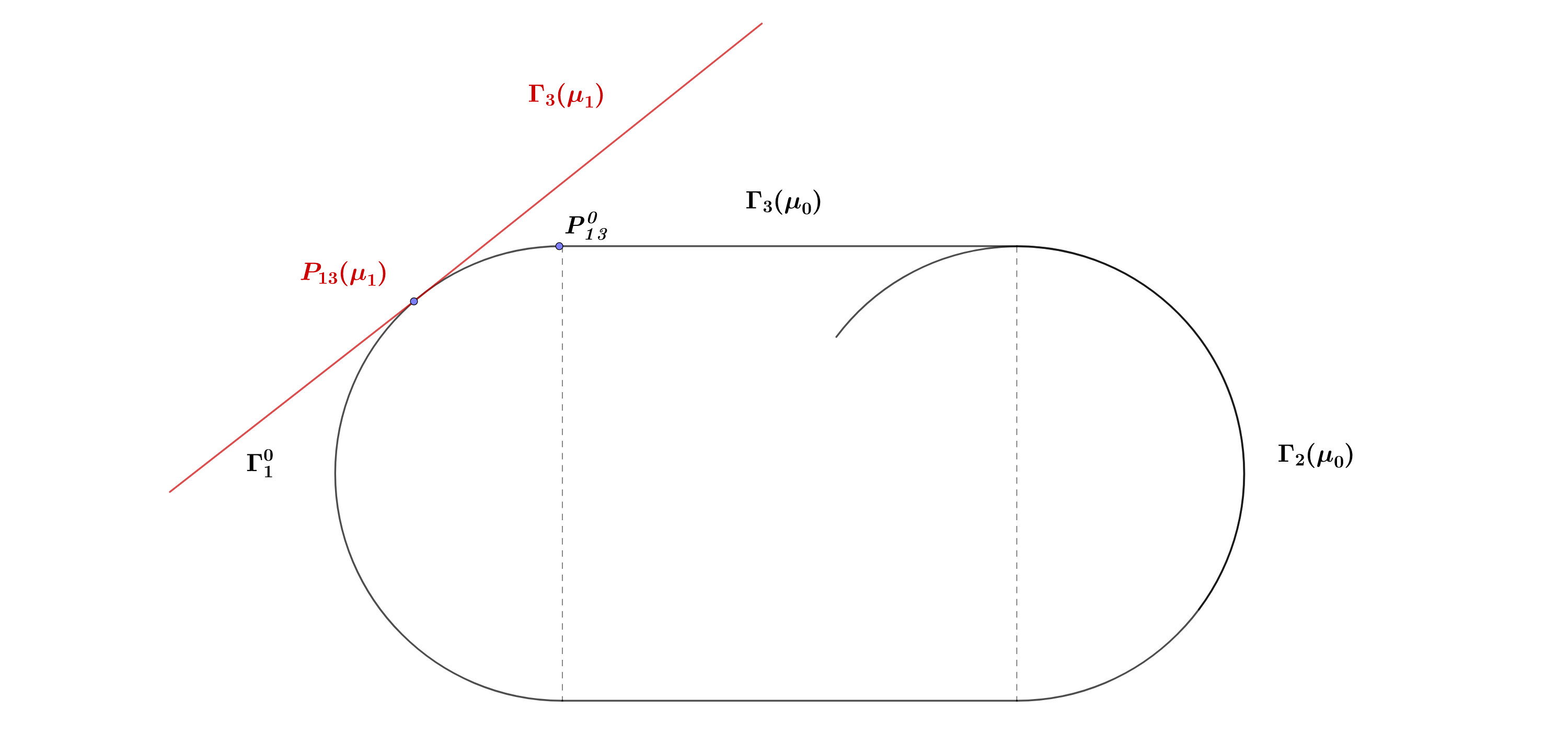
Figure 3: Proof of $P_{14}(\mu)=P_{14}^{0}$

It directly follows that $\Gamma_{i}(\mu)=\Gamma_{i}(0)$, $i=1,2,3,4$, for all $\mu\in[-1,1]$. Hence the normalized family $\left\{\Omega_{\mu}\right\}_{|\mu|\leq 1}$ is a constant family, that is, $\Omega_{\mu}=\Omega_{0}$. Therefore, $\widehat{\Omega}_{\mu}=\mathcal{T}_{\mu}^{-1}\Omega_{\mu}=\mathcal{T}_{\mu}^{-1}\Omega_{0}$, which implies that the original family $\left\{\widehat{\Omega}_{\mu}\right\}_{|\mu|\leq 1}$ is an isometric family. ∎

Let us recall the statement of Squash Rigidity Theorem: for any homothety ratio $\chi>0$, if a family $\left\{\widehat{\Omega}_{\mu}\right\}_{|\mu|\leq 1}$ of Bunimovich squash-type stadia in $\mathcal{M}^{\omega}_{ss}(\chi)$ is dynamically isospectral, then it is an isometric family. By Lemma 5.2, it is sufficient to show that the normalized family $\left\{\Omega_{\mu}\right\}_{|\mu|\leq 1}$ is a constant family, or equivalently, $\mathbf{n}\equiv 0$ on $J_{1}\cup J_{2}$. Note that if the original family $\left\{\widehat{\Omega}_{\mu}\right\}_{|\mu|\leq 1}$ is dynamically isospectral, so is the normalized family $\left\{\Omega_{\mu}\right\}_{|\mu|\leq 1}$ since isometries do not change length spectra. Moreover, the normalized family $\left\{\Omega_{\mu}\right\}_{|\mu|\leq 1}$ still belongs to the class $\mathcal{M}^{\omega}_{ss}(\chi)$. For the rest of this section and Section 6, we shall focus on the normalized family $\left\{\Omega_{\mu}\right\}_{|\mu|\leq 1}$.

5.2 Functionals related to Length Spectra

We first show the following basic fact for the length spectrum of a Bunimovich squash-type stadium.

Lemma 5.3.

For any Bunimovich squash-type stadium $\Omega$, its length spectrum $\mathcal{L}(\Omega)$ has zero Lebesgue measure.

Proof.

The proof is almost the same as that of Lemma 4.1 in [9], with the only difference that the parametrization $\Phi$ of the boundary $\partial\Omega$ is not $C^{2}$ at the four gluing points. Nevertheless, there are at most countably many periodic orbits through those points, and thus $\mathcal{L}(\Omega)$ has zero Lebesgue measure. ∎

By Lemma 5.3 and the intermediate value theorem, we immediately get

Lemma 5.4.

For any continuous function $\Delta:[-1,1]\to{\mathbb{R}}$, if Range$(\Delta)\subset\mathcal{L}(\Omega)$, then $\Delta\equiv$constant.

Now for any Bunimovich squash-type stadium $\Omega$ with boundary $\partial\Omega=\Gamma_{1}\cup\Gamma_{3}\cup\Gamma_{2}\cup\Gamma_{4}$, we would like to construct functionals corresponding to symbolic codes. For any $q\geq 2$, we introduce the length function associated to a symbolic code $\mathbf{i}=(i_{1},i_{2},\dots,i_{q})\in\{1,2,3,4\}^{q}$, that is,

$$L_{\mathbf{i}}(\gamma)=\sum_{k=1}^{q}\tau(r_{k},r_{k+1})$$

for $\gamma=(r_{1},r_{2},\dots,r_{q})$ such that $r_{k}\in\Gamma_{i_{k}}$ for $1\leq k\leq q$, where we set $r_{q+1}=r_{1}$ since $q+1\equiv 1\pmod{q}$. Similar to Lemma 3.1 and Lemma 4.1, we can show that the maximal points of $L_{\mathbf{i}}$ shall either give the maximal periodic orbits corresponding to $\mathbf{i}$, or a singular set containing some gluing points.

Let us now consider a $C^{1}$ one-parameter normalized family $\left\{\Omega_{\mu}\right\}_{|\mu|\leq 1}$ of the Bunimovich squash-type stadia in $\mathcal{M}^{m}_{ss}$, where $m\geq 3$. We say that a symbolic code $\mathbf{i}$ is good for the family $\left\{\Omega_{\mu}\right\}_{|\mu|\leq 1}$ if

• for every $\mu\in[-1,1]$, there exists a unique maximal periodic orbit $\gamma_{\mathbf{i}}(\mu)$ corresponding to $\mathbf{i}$;

• the dependence $\mu\mapsto\gamma_{\mathbf{i}}(\mu)$ is $C^{1}$ smooth.

Then we can define a $C^{1}$ function by

$$\Delta(\mu;\mathbf{i})=L^{\mu}_{\mathbf{i}}(\gamma_{\mathbf{i}}(\mu)),\ \ \text{for any}\ \mu\in[-1,1].$$

Moreover, let us define the function

$$G(\mu;z)=G(\mu;r,\varphi)=\mathbf{n}(\mu,r)\cos\varphi$$ (5.2)

for a collision point $z=(r,\varphi)$, where $\mathbf{n}$ is the deformation function given by (5.1). By Proposition 4.6 in [9], we obtain

$$\frac{1}{2}\Delta^{\prime}(\mu;\mathbf{i})=\frac{1}{2}\partial_{\mu}L^{\mu}_{\mathbf{i}}(\gamma_{\mathbf{i}}(\mu))=\sum_{z\in\gamma_{\mathbf{i}}(\mu)}G(\mu;z).$$ (5.3)

If the family $\left\{\Omega_{\mu}\right\}_{|\mu|\leq 1}$ is dynamically isospectral, that is, $\mathcal{L}(\Omega_{\mu})=\mathcal{L}(\Omega)$ for any $\mu\in[-1,1]$, then $\mu\mapsto\Delta(\mu;\mathbf{i})$ is constant by Lemma 5.4. Therefore, by (5.3),

$$\sum_{z\in\gamma_{\mathbf{i}}(\mu)}G(\mu;z)=0,\ \ \text{for any}\ \ \mu\in[-1,1].$$ (5.4)

We now investigate the unique maximal periodic orbits corresponding to special good codes that we have studied in earlier sections:

• Functionals related to the maximal period two orbit $\gamma^{*}(\mu)$: note that the corresponding symbolic code is $\overline{12}$. Since $\Delta(\mu;\overline{12})$ is constant in $\mu$, and the angles for $\gamma^{*}(\mu)$ are of zero degree, we have for any $\mu\in[-1,1]$,

  $$\frac{1}{2}\Delta^{\prime}(\mu;\overline{12})=\sum_{z\in\gamma^{*}(\mu)}G(\mu;z)=\mathbf{n}_{1}(\mu,0)+\mathbf{n}_{2}(\mu,0).$$ (5.5)

• Functionals related to the palindromic periodic orbits $\gamma_{n}(\mu)$, which are studied in Section 4 for the table $\Omega_{\mu}$. The symbolic codes $\mathbf{i}_{n}$ for $\gamma_{n}(\mu)$ are given by (4.1), and the corresponding functional is given by

  $$\frac{1}{2}\Delta^{\prime}(\mu;\mathbf{i}_{n})=\sum_{z\in\gamma_{n}(\mu)}G(\mu;z).$$

For notational simplicity, we shall omit $\mu$ and just write $\Gamma_{i}$, $\mathbf{n}(r)$, $\gamma^{*}$, $\gamma_{n}$, $G(z)$, instead of $\Gamma_{i}(\mu)$, $\mathbf{n}(\mu,r)$, $\gamma^{*}(\mu)$, $\gamma_{n}(\mu)$, $G(\mu;z)$ respectively. Also, we briefly write the summation $\sum_{z\in\gamma}G(z)$ by $\sum_{\gamma}G$.

5.3 Arclength Parameterization on $\Gamma_{1}$ and $\Gamma_{2}$

Recall that the deformation function $\mathbf{n}=\mathbf{n}_{\Phi}$ would have different formulas under different pararmetrizations $\Phi$. As we have explained in Remark 5.1, Lemma 3.3 in [9] shows that the vanishing property of $\mathbf{n}$ does not depend on the parametrizations at all. In order to apply the formulas that we previously obtained in Section 3 and 4, we shall introduce the parametrizations separately on $\Gamma_{1}(\mu)$ and $\Gamma_{2}(\mu)$ which are of arclength parametrization for some a priori fixed parameter $\mu_{0}$ as follows.

More precisely, we recall that the normalized family $\left\{\Omega_{\mu}\right\}_{|\mu|\leq 1}$ belongs to the class $\mathcal{M}^{m}_{ss}(\chi)$, where $m\geq 3$ and $\chi$ is an a priori fixed homothety ratio. Given a fixed $\mu_{0}\in[-1,1]$, we first introduce a parametrization $s\mapsto\Phi_{1}(\mu,s)$ with $s\in J_{1}$ on $\Gamma_{1}(\mu)$ such that $\Phi_{1}(\mu,0)=A$ for all $\mu\in[-1,1]$ and $\Phi_{1}(\mu_{0},s)$ is of arclength parametrization on $\Gamma_{1}(\mu_{0})$. Recall that the unique maximal period two orbit of $\Omega_{\mu}$ is given by $\gamma^{*}(\Omega_{\mu})=\overline{AB(\mu)}$, where $A$ is the origin of ${\mathbb{R}}^{2}$ and $B(\mu)$ lies on the positive horizontal semiaxis of ${\mathbb{R}}^{2}$. By Assumption (IV), there is an orientation preserving $\chi$-homothety $\mathcal{S}_{\mu}$ transforms a sub-curve of $\Gamma_{1}(\mu)$ near $A$ onto a sub-curve of $\Gamma_{2}(\mu)$ near $B(\mu)$. We note that the tangent (resp. normal) vector of both $\Gamma_{1}(\mu)$ at $A$ and $\Gamma_{2}(\mu)$ at $B(\mu)$ is vertical (resp. horizontal), and $\mathcal{S}_{\mu}$ transforms the tangent/normal vector of $\Gamma_{1}(\mu)$ at $A$ into the tangent/normal vector of $\Gamma_{2}(\mu)$ at $B(\mu)$. Therefore, if we set

$$\widetilde{\Phi}_{2}(\mu,t)=\mathcal{R}_{\mu}\left[\chi\Phi_{1}\left(\mu,t/\chi\right)\right]\ \ \text{for}\ t\ \text{close to}\ 0,$$

where $\mathcal{R}_{\mu}$ is the counter-clockwise rotation with center at the middle point of $\overline{AB(\mu)}$ by 180 degree, then the graph of $\widetilde{\Phi}_{2}(\mu,t)$ coincides with $\Gamma_{2}(\mu)$ near $B(\mu)$. Therefore, we can extend $t\mapsto\widetilde{\Phi}_{2}(\mu,t)$ to a parametrization $t\mapsto\Phi_{2}(\mu,t)$ with $t\in J_{2}$ on $\Gamma_{2}(\mu)$ for all $\mu\in[-1,1]$ such that

$$\Phi_{2}(\mu,t)=\mathcal{R}_{\mu}\left[\chi\Phi_{1}\left(\mu,t/\chi\right)\right]\ \ \text{for}\ t\ \text{close to}\ 0.$$ (5.6)

In particular, we have $\Phi_{2}(\mu,0)=B(\mu)$ for all $\mu\in[-1,1]$ and $\Phi_{2}(\mu_{0},t)$ is of arclength parametrization on $\Gamma_{2}(\mu_{0})$. Of course, the parametrizations $s\mapsto\Phi_{1}(\mu,s)$ and $t\mapsto\Phi_{2}(\mu,t)$ need not be of arclength for other parameters $\mu\neq\mu_{0}$. Under the new parametrizations, we denote the deformation function on $\Gamma_{1}(\mu)$ and $\Gamma_{2}(\mu)$ by $\mathbf{n}_{1}(\mu,s)$ and $\mathbf{n}_{2}(\mu,t)$ respectively. Below is an immediate consequence of the fact that the family $\{\Omega_{\mu}\}_{|\mu|\leq 1}$ is in the normalized position.

Lemma 5.5.

$\mathbf{n}_{1}(\mu,0)=\mathbf{n}_{1}^{\prime}(\mu,0)=0$ for any $\mu\in[-1,1]$.

Proof.

$\Phi_{1}(\mu,0)=A$ implies that $\partial_{\mu}\Phi_{1}(\mu,0)=0$, and hence

$$\mathbf{n}_{1}(\mu,0)=\langle\partial_{\mu}\Phi_{1}(\mu,0),\ N_{1}(\mu,0)\rangle=0.$$

Furthermore, for any $\mu\in[-1,1]$, the tangent vector of $\Gamma_{1}(\mu)$ at $A$, denoted by $\partial_{s}\Phi_{1}(\mu,0)$, is a downward vertical vector at $A$ in ${\mathbb{R}}^{2}$. Here we take the downward direction because $\partial\Omega_{\mu}$ is parametrized along the counter-clockwise direction. Therefore, $\partial_{\mu}\partial_{s}\Phi_{1}(\mu,0)$ is perpendicular to the out-going unit normal vector $N_{1}(\mu,0)$ and hence

$$\mathbf{n}_{1}^{\prime}(\mu,0)=\langle\partial_{\mu}\partial_{s}\Phi_{1}(\mu,0),\ N_{1}(\mu,0)\rangle+\langle\partial_{\mu}\Phi_{1}(\mu,0),\ \partial_{s}N_{1}(\mu,0)\rangle=0.$$

The proof of this lemma is completed. ∎

By Lemma 5.2, the Squash Rigidity Theorem is reduced to showing that $\mathbf{n}(\mu,\cdot)\equiv 0$ on $\Gamma_{1}\cup\Gamma_{2}$ for any $\mu\in[-1,1]$. Since the vanishing property of $\mathbf{n}$ does not depend on the parametrization and the choice of $\mu_{0}$ is arbitrary, it suffices to show that $\mathbf{n}_{1}(\mu_{0},s)=0$ and $\mathbf{n}_{2}(\mu_{0},t)=0$. For simplicity, we shall omit $\mu_{0}$ and simply write $\mathbf{n}_{1}(s)$ and $\mathbf{n}_{2}(t)$. Note that $\mathbf{n}_{1}$ and $\mathbf{n}_{2}$ are both $C^{m}$ smooth.

6 Proof of Squash Rigidity Theorem

6.1 Reduction of Squash Rigidity Theorem

For any homothety ratio $\chi>0$, let $\left\{\widehat{\Omega}_{\mu}\right\}_{|\mu|\leq 1}$ be a $C^{1}$ one-parameter family in $\mathcal{M}^{\omega}_{ss}(\chi)$, and $\left\{\Omega_{\mu}\right\}_{|\mu|\leq 1}$ be its normalized family. As introduced in the previous section, the deformation function is denoted by $\mathbf{n}_{1}(s)$ on $\Gamma_{1}$, and by $\mathbf{n}_{2}(t)$ on $\Gamma_{2}$. Note that both $\mathbf{n}_{1}(s)$ and $\mathbf{n}_{2}(t)$ are analytic. By Lemma 5.2, the Squash Rigidity Theorem is reduced to the following.

Proposition 6.1.

If the family $\left\{\Omega_{\mu}\right\}_{|\mu|\leq 1}$ is dynamically isospectral, then $\mathbf{n}_{1}\equiv 0$ and $\mathbf{n}_{2}\equiv 0$.

Note that the dynamically isospectral property implies (5.4), that is, the sum of $G$ vanishes over the unique maximal periodic orbit $\gamma_{\mathbf{i}}$ which corresponds to a good symbolic code $\mathbf{i}$. In the analytic class $\mathcal{M}^{\omega}_{ss}(\chi)$ of Bunimovich squash-type stadia, it turns out that Condition (5.4) over the period two orbit $\gamma^{*}$ and the palindromic orbits $\gamma_{n}$ are sufficient to establish the dynamical spectral rigidity. More precisely, we have

Proposition 6.2.

If $\sum_{\gamma^{*}}G=\sum_{\gamma_{n}}G=0$ for any $n\geq 1$, then

$$\mathbf{n}_{1}^{(d)}(0)=\mathbf{n}_{2}^{(d)}(0)=0,\ \ \text{for any}\ d\geq 0.$$

We remark that Proposition 6.2 also holds in the class $\mathcal{M}^{\infty}_{ss}(\chi)$. In the analytic class $\mathcal{M}^{\omega}_{ss}(\chi)$, it immediately follows that $\mathbf{n}_{1}$ and $\mathbf{n}_{2}$ both vanish since they are analytic, which proves Proposition 6.1 and thus Squash Rigidity Theorem. In the rest of this section, we prove Proposition 6.2.

6.2 Cancellations by Interpolations

6.2.1 Sums of $G$ over $\gamma_{n}$

Recall that $\gamma_{n}$ is the sequence of palindromic periodic orbits that we introduce in Section 4.1, with collision points

$$y_{n}(0^{-})\mapsto x_{n}(0)\mapsto y_{n}(0)\mapsto x_{n}(1)\mapsto y_{n}(1)\mapsto\dots\mapsto x_{n}(n)\mapsto y_{n}(n)\mapsto x_{n}(n+1).$$

Note that we have $y_{n}(0)=(t_{n}(0),\psi_{n}(0))$ and $y_{n}(0^{-})=(t_{n}(0),-\psi_{n}(0))$. Then
$G(y_{n}(0^{-}))=G(y_{n}(0))$, due to the special formula of $G$, i.e., cosine function for the angle variable. Moreover, the time-reversibility (4.3) implies that

$$\begin{split}G(x_{n}(n+2-k))=G(x_{n}(k)),\ \ &\ \ k=1,\dots,n+1,\\ G(y_{n}(n+1-k))=G(y_{n}(k)),\ \ &\ \ k=1,\dots,n.\end{split}$$ (6.1)

For a sufficiently large integer $\ell>0$ and for any integer $n\geq 2\ell$, we define the global sum and local sum of $G$ over $\gamma_{n}$ as follows.

• Global sum: we define the global sum of $G$ over the points of $\gamma_{n}$ (with minus signs) away from the period two orbit as

  $$\begin{split}S_{n}^{global}(\ell):=&-G(y_{n}(0^{-}))-G(x_{n}(0))-G(y_{n}(0))-\sum_{k=1}^{\ell}\left[G(x_{n}(k))+G(y_{n}(k))\right]\\ &-\sum_{k=1}^{\ell}\left[G(x_{n}(n+2-k))+G(y_{n}(n+1-k))\right]\end{split}$$

  This global sum contains $(4\ell+3)$ points. By (6.1) and the fact that $G(y_{n}(0^{-}))=G(y_{n}(0))$, we get

  $$S_{n}^{global}(\ell)=-G(x_{n}(0))-2G(y_{n}(0))-2\sum_{k=1}^{\ell}\left[G(x_{n}(k))+G(y_{n}(k))\right].$$

• Local sum: we define the local sum of $G$ over the points of $\gamma_{n}$ near the period two orbit as

  $$S_{n}^{local}(\ell):=\sum_{k=\ell+1}^{n-\ell+1}G(x_{n}(k))+\sum_{k=\ell+1}^{n-\ell}G(y_{n}(k)).$$

  Note that the local sum contains $(2n-4\ell+1)$ points. By convention, the above second sum is set to be zero if $n=2\ell$.

By the assumption of Proposition 6.2, i.e., $\sum_{\gamma_{n}}G=0$, we get $-S_{n}^{global}(\ell)+S_{n}^{local}(\ell)=0$. For simplicity, we further denote

$$S_{n}(\ell):=S_{n}^{global}(\ell)=S_{n}^{local}(\ell),$$

and thus $S_{n}(\ell)$ has two expressions:

$$S_{n}(\ell) = -G(x_{n}(0))-2G(y_{n}(0))-2\sum_{k=1}^{\ell}\left[G(x_{n}(k))+G(y_{n}(k))\right]$$ (6.2)

$$= \sum_{k=\ell+1}^{n-\ell+1}G(x_{n}(k))+\sum_{k=\ell+1}^{n-\ell}G(y_{n}(k)).$$ (6.3)

In the next two subsections, we shall introduce the (weighted) Lagrange interpolation method and use it to prove the cancellations for the global sum representation of $S_{n}(\ell)$. Then in Section 6.3, we shall use such cancellations to extract information about the derivatives $\mathbf{n}_{1}^{(d)}(0)$ and $\mathbf{n}_{2}^{(d)}(0)$ by applying the Taylor expansion for the local sum representation of $S_{n}(\ell)$.

6.2.2 Lagrange Polynomial Interpolation and Weighted Interpolation

In this subsection, we first recall the well known Lagrange polynomial interpolation for functions of one variable (see e.g. [24], §6.2). More precisely, for any integer $m\geq 2$ and real numbers $0\leq u_{m}<\dots<u_{1}\leq 1$, the fundamental Lagrange polynomials over the data set $\{u_{1},\dots,u_{m}\}$ are defined by

$$p_{j}(u)=p_{j}(u;u_{1},\dots,u_{m}):=\prod_{\begin{subarray}{c}1\leq i\leq m\\ i\neq j\end{subarray}}\frac{u-u_{i}}{u_{j}-u_{i}}$$ (6.4)

for $u\in{\mathbb{R}}$ and $j=1,\dots,m$. Note that these polynomials stasify the Lagrange basis property, i.e., $p_{j}(u_{j})=1$ and $p_{j}(u_{i})=0$ if $i\neq j$. The Lagrange polynomial interpolation provides an approximation of a $C^{m}$ smooth function in the space of degree $(m-1)$ polynomials, with a higher order error.

Lemma 6.3.

For any function $g\in C^{m}[0,1]$ and for any $u\in[0,1]$, there exists $\overline{u}$ in the smallest interval that contains $u_{1},\dots,u_{m}$ and $u$ such that

$$g(u)=\sum_{j=1}^{m}g(u_{j})p_{j}(u)+\frac{g^{(m)}(\overline{u})}{m!}\prod_{j=1}^{m}(u-u_{j}).$$

We also need the weighted Lagrange interpolation, which can be regarded as a variant of the standard Lagrange polynomial interpolation (see e.g. [2]). More precisely, let $w\in C^{m}[0,1]$ be a positive function, and define the fundamental weighted Lagrange interpolants over the data set $\{u_{1},\dots,u_{m}\}$ by

$$q_{j}(u)=q_{j}(u;u_{1},\dots,u_{m};w):=\frac{w(u_{j})}{w(u)}p_{j}(u;u_{1},\dots,u_{m}),$$ (6.5)

for $u\in{\mathbb{R}}$ and $j=1,\dots,m$, where $p_{j}(u;u_{1},\dots,u_{m})$ is the standard fundamental Lagrange polynomials given by (6.5). Note that we still have the basis property for $\{q_{j}(u)\}_{1\leq j\leq m}$. In particular case when $w\equiv 1$, we have that $q_{j}(u)=p_{j}(u)$.

Appying Lemma 6.3 for the function $w(u)g(u)$ and then dividing $w(u)$ on both sides, we obtain the weighted Lagrange interpolation as follows.

Lemma 6.4.

For any function $g\in C^{m}[0,1]$ and for any $u\in[0,1]$, there exists $\overline{u}$ in the smallest interval that contains $u_{1},\dots,u_{m}$ and $u$ such that

$$g(u)=\sum_{j=1}^{m}g(u_{j})q_{j}(u)+\frac{(wg)^{(m)}(\overline{u})}{m!w(u)}\prod_{j=1}^{m}(u-u_{j}).$$

Remark 6.5.

The Lagrange interpolation, either polynomial or weighted, heavily depends on the distributions of data points $u_{1},\dots,u_{m}$. For our purpose, we shall consider geometric data points, i.e., $u_{j}=\lambda^{-j}u_{0}$ for some $u_{0}\in(0,1]$. Putting $u=u_{0}$ in (6.4), we notice that $q_{j}(u_{0})$, $j=1,\dots,m$, are in fact constants (for our special choices of $w_{m}(u)$ in (6.6)), and hence we shall obtain a linear combination of the function values $g(u_{0}),g(u_{1}),\dots,g(u_{m})$ up to a higher order error.

6.2.3 Cancellations by Lagrange Interpolations

We now apply the weighted Lagrange interpolation to show the following cancellations for a linear combination of $\{S_{2\ell+j}(\ell)\}_{0\leq j\leq m}$. The key observation is from Lemma 4.6, which suggests that for each $1\leq k\leq\ell$, the points $\{x_{2\ell+j}(k)\}_{0\leq j\leq m}$ (resp. the points $\{y_{2\ell+j}(k)\}_{0\leq j\leq m}$ for each $k=0^{\pm},0,1,\dots$) are asymptotically lying on a line. In the following applications, we choose the weighted function to be

$$w_{m}(u)=1\text{ if $m$ is odd};\,\,\,\,\,w_{m}(u)=u\text{ if $m$ is even}.$$ (6.6)

Lemma 6.6.

For any integer $m\geq 2$ and sufficiently large $\ell\geq 1$, we have

$$\sum_{j=0}^{m}A_{m,j}w_{m}(\lambda^{-j})S_{2\ell+j}(\ell)=\mathcal{O}\left(\lambda^{-m\ell}\right),$$ (6.7)

where

$$A_{m,0}=-1,\ \text{and}\ A_{m,j}=\prod_{\begin{subarray}{c}1\leq i\leq m\\ i\neq j\end{subarray}}\frac{\lambda^{i}-1}{\lambda^{i-j}-1},\ \ \text{for}\ j=1,\dots,m.$$ (6.8)

Proof.

For any $\ell\geq 1$ and $1\leq k\leq\ell$, we set $u_{j}=u_{j}(k,\ell):=\lambda^{k-2\ell-j}$ for $j=0,1,\dots,m$. By Lemma 4.6, we have

$$x_{2\ell+j}(k)-x_{\infty}(k)=u_{j}\left[v_{\infty}(2k)+o(1)\right].$$

This expression means that the points $\{x_{2\ell+j}(k)\}_{0\leq j\leq m}$ asymptotically lie on the straight line which goes through $x_{\infty}(k)$ and has direction vector $v_{\infty}(2k)$. Recall that $M$ is the phase space defined in (1.2). We then define a piecewise linear curve $\sigma_{0}:[0,u_{0}]\to M$ by setting

$$\sigma_{0}(0)=x_{\infty}(k),\ \ \text{and}\ \ \sigma_{0}(u_{j})=x_{2\ell+j}(k),\ \text{for}\ j=0,1,\dots,m,$$

and connect two consecutive points by line segments. Then

$$|\sigma_{0}^{\prime}(u)|\leq 2\left\|v_{\infty}(2k)\right\|,\ \ \text{and}\ \ |\sigma_{0}^{(i)}(u)|=0\ \text{for}\ i\geq 2,$$

for all $u\in[0,u_{0}]$ except at possibly corner points $u_{j}$ for $j=1,\dots,m$. Moreover, for sufficiently large $\ell\geq 1$, the angle at each corner point can be made very obtuse and close to $180$ degree.

For any $\varepsilon>0$, we can obtain a $C^{\infty}$ smooth curve $\sigma_{\varepsilon}:[0,u_{0}]\to M$ by smoothening the curve $\sigma_{0}$ near these corner points, such that

• $\sigma_{\varepsilon}$ uniformly converges to $\sigma_{0}$ in the $C^{0}$ topology. In particular, $\sigma_{\varepsilon}(0)=x_{\infty}(k)$, $\sigma_{\varepsilon}(u_{0})=x_{2\ell}(k)$, and $\sigma_{\varepsilon}(u_{j})\to x_{2\ell+j}(k)$ as $\varepsilon\to 0$ for $1\leq j\leq m$.

• $\sigma_{\varepsilon}$ is $C^{\infty}$ flat at the point $u=0$, i.e., $\sigma_{\varepsilon}^{(n)}(0)$ vanishes for any $n\geq 1$.

• there is a constant $D_{m}>0$, which only depends on $m$, such that the derivatives of $\sigma_{\varepsilon}$ are uniformly bounded by $D_{m}$ up to order $m+1$.

Let $\{q_{j}(u)\}_{1\leq j\leq m}$ be the fundamental weighted Lagrange interpolants on the data set $\{u_{1},\dots,u_{m}\}$ given by (6.5), where the polynomials $\{p_{j}(u)\}_{1\leq j\leq m}$ are given by (6.4) and the weight function $w_{m}$ is defined as in (6.6). It is straightforward to verify that $p_{j}(u_{0})=A_{m,j}$, which are given by (6.8). Also, $\dfrac{w_{m}(u_{j})}{w_{m}(u_{0})}=w_{m}(\lambda^{-j})$ and thus $q_{j}(u_{0})=A_{m,j}w_{m}(\lambda^{-j})$.

We now consider the smooth function $g_{\varepsilon}:[0,u_{0}]\to{\mathbb{R}}$ given by $g_{\varepsilon}(u)=G\circ\sigma_{\varepsilon}(u).$ Applying Lemma 6.4 to this function with evaluation at $u=u_{0}$, there exists $\overline{u}\in[0,u_{0}]$ such that

$$g_{\varepsilon}(u_{0}) = \sum_{j=1}^{m}A_{m,j}w_{m}(\lambda^{-j})g_{\varepsilon}(u_{j})+\frac{(w_{m}g_{\varepsilon})^{(m)}(\overline{u})}{m!w_{m}(u_{0})}\prod_{j=1}^{m}(u_{0}-u_{j})$$ (6.9)

$$= \sum_{j=1}^{m}A_{m,j}w_{m}(\lambda^{-j})g_{\varepsilon}(u_{j})+\mathcal{O}\left(\lambda^{m(k-2\ell)}\right).$$

The above error estimate for the last term is due to the following facts:

• $|u_{0}-u_{j}|\leq u_{0}=\lambda^{k-2\ell}$ and thus $\left|\prod\limits_{j=1}^{m}(u_{0}-u_{j})\right|\leq m\lambda^{k-2\ell}$;

• if $m$ is odd, then $w_{m}(u)\equiv 1$ and thus

  $$\left|\frac{(w_{m}g_{\varepsilon})^{(m)}(\overline{u})}{m!w_{m}(u_{0})}\right|\leq\|(g_{\varepsilon})^{(m)}\|_{\infty}\leq\|G\|_{C^{m}}\cdot m^{m}\max\{1,\|\sigma_{\varepsilon}\|_{C^{m}}\}^{m}\leq m^{m}D_{m}^{m}\|G\|_{C^{m}};$$

  if $m$ is even, then $w_{m}(u)\equiv u$. We notice that $\overline{u}\leq u_{0}$, and
  $g_{\varepsilon}^{(m-1)}(0)=(G\circ\sigma_{\varepsilon})^{(m-1)}(0)=0$. Since $\sigma_{\varepsilon}$ is $C^{\infty}$ flat at $u=0$, then we have

  $$\left|\frac{(w_{m}g_{\varepsilon})^{(m)}(\overline{u})}{m!w_{m}(u_{0})}\right| = \left|\frac{\overline{u}g_{\varepsilon}^{(m)}(\overline{u})+mg_{\varepsilon}^{(m-1)}(\overline{u})}{m!u_{0}}\right|\leq\left|g_{\varepsilon}^{(m)}(\overline{u})\right|+\left|\frac{g_{\varepsilon}^{(m-1)}(\overline{u})}{\overline{u}}\right|$$

  $$\leq 2\|(g_{\varepsilon})^{(m)}\|_{\infty}\leq 2m^{m}D_{m}^{m}\|G\|_{C^{m}}.$$

Letting $\varepsilon\to 0$ in (6.9), we get

$$-G(x_{2\ell+j}(k))+\sum_{j=1}^{m}A_{m,j}w_{m}(\lambda^{-j})G(x_{2\ell+j}(k))=\mathcal{O}\left(\lambda^{m(k-2\ell)}\right).$$

In a similar fashion, we also have for any $k=0^{\pm},0,1,\dots,\ell$,

$$-G(y_{2\ell+j}(k))+\sum_{j=1}^{m}A_{m,j}w_{m}(\lambda^{-j})G(y_{2\ell+j}(k))=\mathcal{O}\left(\lambda^{m(k-2\ell)}\right).$$

Therefore, by the definition of $S_{2\ell+j}(\ell)$ given in (6.2), we obtain (6.7) by noticing that the error term is $2\sum_{k=0}^{\ell}\mathcal{O}\left(\lambda^{m(k-2\ell)}\right)=\mathcal{O}\left(\lambda^{-m\ell}\right)$. ∎

We shall need the following property for the coefficients $A_{m,j}$ given in (6.8).

Lemma 6.7.

The coefficients $\{A_{m,j}\}_{0\leq j\leq m}$ in (6.8) satisfy the following properties:

1. For any $0\leq k\leq m-1$,

   $$\sum_{j=0}^{m}A_{m,j}\lambda^{-kj}=0.$$ (6.10)

   Furthermore,

   $$\sum_{j=0}^{m}A_{m,j}\lambda^{-mj}\neq 0.$$ (6.11)

2. For any $0\leq k<m$,

   $$\sum_{j=0}^{m}\ jA_{m,j}\lambda^{-kj}\neq 0.$$ (6.12)

Proof.

Let $\{e_{j}(u)\}_{1\leq j\leq m}$ be the fundamental Lagrange polynomials over the data set $\{\lambda^{-1},\dots,\lambda^{-m}\}$, and notice that $A_{m,j}=e_{j}(1)$ for $j=1,\dots,m$. Recall that $A_{m,0}=-1$. Applying Lemma 6.3 for functions $g(u)=u^{k}$ for any $k\geq 0$, and evaluating at $u=1$, there is $\overline{u}\in[\lambda^{-1},1]$ such that

$$\sum_{j=0}^{m}A_{m,j}\lambda^{-kj} = -\frac{(u^{k})^{(m)}|_{u=\overline{u}}}{m!}\prod_{j=1}^{m}(1-\lambda^{-j})$$

$$= \begin{cases}0,\ &\ \mathrm{if}\ 1\leq k\leq m-1,\\ \prod\limits_{j=1}^{m}(1-\lambda^{-j})\neq 0,\ &\ \mathrm{if}\ k=m.\end{cases}$$

Therefore, (6.10) and (6.11) hold.

Similarly, applying Lemma 6.3 for the set of functions $g(u)=u^{k}\log u$ for any $k\geq 0$, and evaluating at $u=1$, there is $\overline{u}\in[\lambda^{-1},1]$ such that

$$\sum_{j=0}^{m}A_{m,j}\lambda^{-kj}\log\lambda^{-j} = -\frac{(u^{k}\log u)^{(m)}|_{u=\overline{u}}}{m!}\prod_{j=1}^{m}(1-\lambda^{-j})$$

$$= -\frac{(-1)^{m-k-1}k!(m-k-1)!\overline{u}^{k-m}}{m!}\prod_{j=1}^{m}(1-\lambda^{-j})\neq 0.$$

Dividing both sides by $-\log\lambda$, we get (6.12). ∎

6.3 Proof of Proposition 6.2

Recall that in the assumptions of Proposition 6.2, we are dealing with a normalized family $\left\{\Omega_{\mu}\right\}_{|\mu|\leq 1}$ of Bunimovich squash-type stadia in $\mathcal{M}_{ss}^{\omega}(\chi)$, which satisfies that $\sum_{\gamma^{*}}G=\sum_{\gamma_{n}}G=0$ for any $n\geq 1$. We have the following lemma.

Lemma 6.8.

$\mathbf{n}_{1}(0)=\mathbf{n}_{2}(0)=\mathbf{n}_{1}^{\prime}(0)=\mathbf{n}_{2}^{\prime}(0)=0.$

Proof.

We already get that $\mathbf{n}_{1}(0)=\mathbf{n}_{1}^{\prime}(0)=0$ by Lemma 5.5. The assumption that $\sum_{\gamma^{*}}G=0$ yields that $\mathbf{n}_{1}(0)+\mathbf{n}_{2}(0)=0$, and thus $\mathbf{n}_{2}(0)=0$. It also implies that the length function $\Delta(\mu;\overline{12})$ given by (5.5) is constant, which means that $B(\mu)=B$ for any $\mu\in[-1,1]$. Then applying the same arguments in the proof of Lemma 5.5, we get $\mathbf{n}_{2}^{\prime}(0)=0$. ∎

A by-product of the proof of Lemma 6.8 is that $B(\mu)=B$ for any $\mu\in[-1,1]$. Combining with Assumption (IV) with homothety ratio $\chi$, we have the following relation between the derivatives of $\mathbf{n}_{1}$ and $\mathbf{n}_{2}$ at zero.

Lemma 6.9.

$\mathbf{n}_{2}^{(d)}(0)=\chi^{1-d}\mathbf{n}_{1}^{(d)}(0)$ for any $d\geq 0$.

Proof.

In Subsection 5.3, we introduce the parametrizations $s\mapsto\Phi_{1}(\mu,s)$ on $\Gamma_{1}(\mu)$ and $t\mapsto\Phi_{2}(\mu,t)$ on $\Gamma_{2}(\mu)$. Since now $B(\mu)=B$ for any $\mu\in[-1,1]$, by (5.6), we have

$$\Phi_{2}(\mu,t)=\mathcal{R}\left[\chi\Phi_{1}\left(\mu,t/\chi\right)\right]\ \ \text{for}\ t\ \text{close to}\ 0,$$

where $\mathcal{R}$ is the counter-clockwise rotation with center at the middle point of $\overline{AB}$ by 180 degree. By the definition of the deformation function given in (5.1), for any $t$ close to $0$, we have

$$\mathbf{n}_{2}(\mu,t)=\langle\partial_{\mu}\Phi_{2}(\mu,t),\ N_{2}(\mu,t)\rangle=\langle\mathcal{R}\left[\chi\partial_{\mu}\Phi_{1}\left(\mu,t/\chi\right)\right],\mathcal{R}N_{1}(\mu,t/\chi)\rangle=\chi\mathbf{n}_{1}\left(\mu,t/\chi\right),$$

and hence $\mathbf{n}_{2}^{(d)}(0)=\chi^{1-d}\mathbf{n}_{1}^{(d)}(0)$ by taking the $d$-th order derivative at $t=0$. ∎

We are now ready to prove Proposition 6.2 by induction. Note that the base of the induction has already been proven in Lemma 6.8, that is,

$$\mathbf{n}_{1}(0)=\mathbf{n}_{2}(0)=\mathbf{n}_{1}^{\prime}(0)=\mathbf{n}_{2}^{\prime}(0)=0.$$

Suppose now $d\geq 2$ is an integer such that

$$\mathbf{n}_{1}^{(k)}(0)=0\ \text{ and }\ \mathbf{n}_{2}^{(k)}(0)=0,\ \ \text{for any}\ k=0,1,\dots,d-1.$$

We shall use the assumption that $\sum_{\gamma_{n}}G=0$ to show that $\mathbf{n}_{1}^{(d)}(0)=0$ and $\mathbf{n}_{2}^{(d)}(0)=0$.

Recall that the maximal period two orbit is denoted as $\gamma^{*}=\overline{xy}$. Also, $x=(0,0)$ in the $(s,\varphi)$-coordinate and $y=(0,0)$ in the $(t,\psi)$-coordinate. For $z=(s,\varphi)$ near $x=(0,0)$, we write the Taylor expansion of $\mathbf{n}_{1}(s)$ up to the $d$-th order, as well as that of $\cos\varphi$ up to the 1st order as

$$\mathbf{n}_{1}(s)=\frac{1}{d!}\,\mathbf{n}_{1}^{(d)}(0)\,s^{d}+\mathcal{O}\left(s^{d+1}\right),\ \ \cos\varphi=1+\mathcal{O}(\varphi^{2}).$$ (6.13)

Similarly, for $z=(t,\psi)$ near $y=(0,0)$,

$$\mathbf{n}_{2}(t)=\frac{1}{d!}\,\mathbf{n}_{2}^{(d)}(0)\,t^{d}+\mathcal{O}\left(t^{d+1}\right),\ \ \cos\psi=1+\mathcal{O}(\psi^{2}).$$ (6.14)

Given an fixed $j\geq 0$, by Lemma 4.4, we have that for any large $\ell$ and any $i=1,\dots,j+1$,

$$x_{2\ell+j}(\ell+i) =\lambda^{-\ell-i}(C_{s},C_{\varphi})+\lambda^{-\ell+i-j}(C_{s,\ell+i},C_{\varphi,\ell+i})$$

$$+\mathcal{O}\left(\max\left\{\lambda^{-1.5(\ell+i)},\lambda^{1.25(-\ell+i-j)}\right\}\right)$$

$$=\lambda^{-\ell}\left(C_{s}\left(\lambda^{-i}+\lambda^{i-j-2}\right),C_{\varphi}(\lambda^{-i}-\lambda^{i-j-2})\right)+\mathcal{O}(\lambda^{-1.25\ell}).$$

Note that the first term is of leading order $\lambda^{-\ell}$ (as $\ell\to\infty$). Then by (6.13),

$$\begin{split}G(x_{2\ell+j}(\ell+i))&=\mathbf{n}_{1}(s_{2\ell+j}(\ell+i))\cos\left(\varphi_{2\ell+j}(\ell+i)\right)\\ &=\frac{1}{d!}\mathbf{n}_{1}^{(d)}(0)\lambda^{-d\ell}C_{s}^{d}\left(\lambda^{-i}+\lambda^{i-j-2}\right)^{d}+\mathcal{O}\left(\lambda^{-\ell(d+0.25)}\right)\end{split}$$ (6.15)

Similarly, for any $j\geq 1$, $i=1,\dots,j$,

$$G(y_{2\ell+j}(\ell+i))=\frac{1}{d!}\mathbf{n}_{2}^{(d)}(0)\lambda^{-d\ell}C_{t}^{d}\left(\lambda^{-i}+\lambda^{i-j-1}\right)^{d}+\mathcal{O}\left(\lambda^{-\ell(d+0.25)}\right).$$ (6.16)

Applying Lemma 6.6 for $m=d+1$ and sufficiently large $\ell\geq 1$, we obtain

$$\sum_{j=0}^{d+1}A_{d+1,j}w_{d+1}(\lambda^{-j})S_{2\ell+j}(\ell)=\mathcal{O}(\lambda^{-\ell(d+1)}),$$ (6.17)

where $A_{d+1,j}$ are given by (6.8) and $w_{d+1}(\cdot)$ is given by (6.6). Under the assumption that $\sum_{\gamma_{n}}G=0$, we have an alternative formula for $S_{2\ell+j}(\ell)$ given by (6.3), that is,

$$S_{2\ell+j}(\ell)=\sum_{i=1}^{j+1}G(x_{2\ell+j}(\ell+i))+\sum_{i=1}^{j}G(y_{2\ell+j}(\ell+i)).$$

By (6.15) and (6.16), we rewrite the LHS of (6.17) as

$$\sum_{j=0}^{d+1}A_{d+1,j}S_{2\ell+j}(\ell)=\frac{\lambda^{-d\ell}}{d!}\left[\mathcal{A}_{1}C_{s}^{d}\mathbf{n}_{1}^{(d)}(0)+\mathcal{A}_{2}C_{t}^{d}\mathbf{n}_{2}^{(d)}(0)\right]+\mathcal{O}\left(\lambda^{-\ell(d+0.25)}\right),$$

where the coefficients $\mathcal{A}_{\sigma}=\mathcal{A}_{\sigma}(d,\lambda)$, $\sigma=1,2$, are given by

$$\mathcal{A}_{\sigma}=\sum_{j=0}^{d+1}A_{d+1,j}w_{d+1}(\lambda^{-j})\sum_{i=1}^{j+2-\sigma}\left(\lambda^{-i}+\lambda^{i-j-3+\sigma}\right)^{d}.$$ (6.18)

Therefore, multiplying both sides of (6.17) by $\lambda^{d\ell}$ and letting $\ell\to\infty$, we get

$$\mathcal{A}_{1}C_{s}^{d}\mathbf{n}_{1}^{(d)}(0)+\mathcal{A}_{2}C_{t}^{d}\mathbf{n}_{2}^{(d)}(0)=0.$$ (6.19)

The relation between $\mathcal{A}_{1}$ and $\mathcal{A}_{2}$ are given by the following lemma.

Lemma 6.10.

The coefficients $\mathcal{A}_{1}$ and $\mathcal{A}_{2}$ in (6.19) satisfy the following relation:

$$\mathcal{A}_{2}=\lambda^{d/2}\mathcal{A}_{1}\neq 0,\ \text{when}\ d\ \text{is even};\ \ \ \mathcal{A}_{2}=\lambda^{d}\mathcal{A}_{1}\neq 0,\ \text{when}\ d\ \text{is odd}.$$

Proof.

When $d$ is even, we note that $w_{d+1}\equiv 1$. By (6.10), (6.12) and (6.18), we get

$$\mathcal{A}_{\sigma} =\sum_{j=0}^{d+1}A_{d+1,j}\sum_{i=1}^{j+2-\sigma}\sum_{\nu=0}^{d}{d\choose\nu}\lambda^{-i(d-\nu)+\nu(i-j-3+\sigma)}$$

$$=\sum_{\nu=0}^{d}{d\choose\nu}\sum_{j=0}^{d+1}A_{d+1,j}\sum_{i=1}^{j+2-\sigma}\lambda^{-i(d-2\nu)-\nu(j+3-\sigma)}$$

$$=\sum_{\nu=0}^{d}{d\choose\nu}\sum_{j=0}^{d+1}A_{d+1,j}\cdot\begin{cases}\dfrac{\lambda^{-(d-2\nu)-\nu(j+3-\sigma)}-\lambda^{-(d-\nu)(j+3-\sigma)}}{1-\lambda^{-(d-2\nu)}},&\ \mathrm{if}\ \nu\neq d/2,\\ \\ (j+2-\sigma)\lambda^{-\nu(j+3-\sigma)},&\ \mathrm{if}\ \nu=d/2,\end{cases}$$

$$=\sum_{\nu=0}^{d}{d\choose\nu}\cdot\begin{cases}0,&\ \mathrm{if}\ \nu\neq d/2,\\ \\ \sum_{j=0}^{d+1}jA_{d+1,j}\lambda^{-\nu(j+3-\sigma)},&\ \mathrm{if}\ \nu=d/2,\end{cases}$$

$$=\lambda^{-d(3-\sigma)/2}{d\choose d/2}\sum_{j=0}^{d+1}jA_{d+1,j}\lambda^{-dj/2}\neq 0,$$

where the last term came from the only non-trivial term with $\nu=d/2$. Therefore, $\mathcal{A}_{2}=\lambda^{d/2}\mathcal{A}_{1}\neq 0$.

When $d$ is odd, we note that $w_{d+1}(u)=u$ and thus $w_{d+1}(\lambda^{-j})=\lambda^{-j}$. By (6.10), (6.11) and (6.18), we have

$$\mathcal{A}_{\sigma} = \sum_{j=0}^{d+1}A_{d+1,j}\lambda^{-j}\sum_{i=1}^{j+2-\sigma}\sum_{\nu=0}^{d}{d\choose\nu}\lambda^{-i(d-\nu)+\nu(i-j-3+\sigma)}$$

$$= \sum_{\nu=0}^{d}{d\choose\nu}\sum_{j=0}^{d+1}A_{d+1,j}\lambda^{-j}\sum_{i=1}^{j+2-\sigma}\lambda^{-i(d-2\nu)-\nu(j+3-\sigma)}$$

$$= \sum_{\nu=0}^{d}{d\choose\nu}\sum_{j=0}^{d+1}A_{d+1,j}\lambda^{-j}\cdot\dfrac{\lambda^{-(d-2\nu)-\nu(j+3-\sigma)}-\lambda^{-(d-\nu)(j+3-\sigma)}}{1-\lambda^{-(d-2\nu)}}$$

$$= \sum_{\nu=0}^{d}{d\choose\nu}\dfrac{\mathcal{A}_{\sigma}^{1}(\nu)-\mathcal{A}_{\sigma}^{2}(\nu)}{1-\lambda^{-(d-2\nu)}},$$

where

$$\mathcal{A}_{\sigma}^{1}(\nu) = \lambda^{-(d-2\nu)-\nu(3-\sigma)}\sum_{j=0}^{d+1}A_{d+1,j}\lambda^{-(\nu+1)j},$$

$$= \lambda^{-(d-2\nu)-\nu(3-\sigma)}\cdot\begin{cases}0,\ &\ \mathrm{if}\ 0\leq\nu<d,\\ \\ \sum\limits_{j=0}^{d+1}A_{d+1,j}\lambda^{-(d+1)j},\ &\ \mathrm{if}\ \nu=d,\end{cases}$$

and

$$\mathcal{A}_{\sigma}^{2}(\nu) = \lambda^{-(d-\nu)(3-\sigma)}\sum_{j=0}^{d+1}A_{d+1,j}\lambda^{-(d+1-\nu)j}$$

$$= \lambda^{-(d-\nu)(3-\sigma)}\cdot\begin{cases}0,\ &\ \mathrm{if}\ 1\leq\nu\leq d,\\ \\ \sum\limits_{j=0}^{d+1}A_{d+1,j}\lambda^{-(d+1)j},\ &\ \mathrm{if}\ \nu=0.\end{cases}$$

Therefore,

$$\mathcal{A}_{\sigma}=\dfrac{\mathcal{A}^{1}_{\sigma}(d)}{1-\lambda^{d}}-\dfrac{\mathcal{A}^{2}_{\sigma}(0)}{1-\lambda^{-d}} = \left(\dfrac{\lambda^{d(\sigma-2)}}{1-\lambda^{d}}-\dfrac{\lambda^{d(\sigma-3)}}{1-\lambda^{-d}}\right)\sum\limits_{j=0}^{d+1}A_{d+1,j}\lambda^{-(d+1)j}$$

$$= \dfrac{2\lambda^{d(\sigma-2)}}{1-\lambda^{d}}\sum\limits_{j=0}^{d+1}A_{d+1,j}\lambda^{-(d+1)j},$$

which implies that $\mathcal{A}_{2}=\lambda^{d}\mathcal{A}_{1}\neq 0$. ∎

By (6.19) and Lemma 6.10, we get that for any $d\geq 2$,

$$C_{s}^{d}\,\mathbf{n}_{1}^{(d)}(0)+\lambda^{d\beta(d)}\,C_{t}^{d}\,\mathbf{n}_{2}^{(d)}(0)=0,$$ (6.20)

where we set $\beta(d)=\frac{1}{2}$ when $d$ is even and $\beta(d)=1$ when $d$ is odd. By Lemma 6.9 which asserts that $\mathbf{n}_{2}^{(d)}(0)=\chi^{1-d}\mathbf{n}_{1}^{(d)}(0)$, we further get

$$C_{s}^{d}\left[1+\lambda^{d\beta(d)}\left(C_{t}/C_{s}\right)^{d}\chi^{1-d}\right]\cdot\mathbf{n}_{1}^{(d)}(0)=0.$$ (6.21)

Recall that $C_{s}$ and $C_{t}$ are computed in (4.6) of Lemma 4.4, then we have $C_{s}\neq 0$ and $C_{t}/C_{s}=-\frac{2a_{1}}{1+\lambda}>0$ since $a_{1}<-1$ and $\lambda>1$. Hence

$$C_{s}^{d}\left[1+\lambda^{d\beta(d)}\left(C_{t}/C_{s}\right)^{d}\chi^{1-d}\right]\neq 0,$$

which implies that $\mathbf{n}_{1}^{(d)}(0)=0$ and thus $\mathbf{n}_{2}^{(d)}(0)=\chi^{1-d}\mathbf{n}_{1}^{(d)}(0)=0$ as well.

Now that we have shown that no matter $d$ is even or odd, we always have that $\mathbf{n}_{1}^{(d)}(0)=\mathbf{n}_{2}^{(d)}(0)=0$, and so the proof of Proposition 6.2 is complete. As we are in the setting of the analytic class $\mathcal{M}^{\omega}_{ss}(\chi)$, Proposition 6.2 implies that $\mathbf{n}_{1}$ and $\mathbf{n}_{2}$ both vanish, which proves Proposition 6.1 and thus Squash Rigidity Theorem.

7 Proof of the Stadium Rigidity Theorem

Let $\{\Omega_{\mu}\}_{|\mu|\leq 1}$ be a $C^{1}$ family of Bunimovich stadia in $\mathcal{M}^{\omega}_{s,b}$, such that the flat boundaries $\Gamma_{3}$ and $\Gamma_{4}$ are two opposite sides of a fixed rectangle. We also denote the arcs by $\Gamma_{i}=\Gamma_{i}(\mu)$, $i=1,2$. As the flat boundaries are a priori fixed, the four gluing points do not depend on the parameter $\mu$, and thus we could denote the gluing points by

$$P_{ij}:=\Gamma_{i}(\mu)\cap\Gamma_{j},\ \ i=1,2,\ j=3,4.$$

The absolute curvature of $\Gamma_{i}=\Gamma_{i}(\mu)$ at the gluing point $P_{ij}$ is denoted by $\mathcal{K}_{ij}=\mathcal{K}_{ij}(\mu)$. Since $\Omega_{\mu}\in\mathcal{M}^{\omega}_{s,b}$, in particular, $\Omega_{\mu}$ satisfies Assumption (II), i.e., $\partial\Omega_{\mu}$ is not $C^{2}$ smooth at these gluing points, then we must have $\mathcal{K}_{ij}>0$.

Note that $\overline{P_{14}P_{13}P_{23}P_{24}}$ is a rectangle, and we denote

$$Q:=\frac{|\overline{P_{13}P_{23}}|}{|\overline{P_{14}P_{13}}|}.$$ (7.1)

The Stadium Rigidity Theorem concerns the dynamical spectral rigidity in the class $\mathcal{M}^{\omega}_{s,b}$. With careful arrangement, we choose a parametrization $\Phi:[-1,1]\times J\to{\mathbb{R}}^{2}$ for the family of stadia $\left\{\Omega_{\mu}\right\}_{|\mu|\leq 1}$ along the counter-clockwise direction, where

$$J=[0,|\partial\Omega_{0}|]:=J_{1}\cup J_{3}\cup J_{2}\cup J_{4},$$

such that

• For any $\mu\in[-1,1]$ and $i=1,2,3,4$, we have $\Phi(\mu,J_{i})=\Gamma_{i}(\mu)$. In particular, $\Gamma_{j}(\mu)=\Gamma_{j}$ for $j=3,4$. Also, $\Phi(\mu,0)=P_{14}$ and $\Phi(\mu,|J_{1}|+|J_{3}|)=P_{23}$;

• The mapping $\mu\mapsto\Phi(\mu,\cdot)$ is $C^{1}$ smooth;

• Set $\Phi_{i}=\Phi|_{J_{i}}$ for $i=1,2$. For any fixed $\mu\in[-1,1]$, the map $r\mapsto\Phi_{i}(\mu,r)$ is analytic.

• As the flat boundaries $\Gamma_{3}$ and $\Gamma_{4}$ are fixed, we could also assume that

  $$\Phi(\mu,r)=\Phi(0,r),\ \text{for any}\ \mu\in[-1,1]\ \text{and}\ r\in J_{3}\cup J_{4}.$$ (7.2)

We then define the deformation function $\mathbf{n}:[-1,1]\times J\to{\mathbb{R}}$ as in (5.1). It is obvious that $\mathbf{n}\equiv 0$ on $[-1,1]\times\left(J_{3}\cup J_{4}\right)$. Moreover, for any $\mu\in[-1,1]$, the function $r\to\mathbf{n}(\mu,r)$ is analytic on $J_{1}\cup J_{2}$.

For brevity, when the parameter $\mu$ is clear, we shall just write $\mathbf{n}(r)$ instead of $\mathbf{n}(\mu,r)$. From Section 5.2, we know that if the family of domains $\left\{\Omega_{\mu}\right\}_{|\mu|\leq 1}$ is dynamically isospectral, then

$$\sum_{z\in\gamma}G(z)=\sum_{(r,\varphi)\in\gamma}\mathbf{n}(r)\cos\varphi=0,$$ (7.3)

for any periodic billiard orbit $\gamma$. Since $\mathbf{n}\equiv 0$ on $J_{3}\cup J_{4}$, the equation (7.3) holds for any periodic trajectories of the induced billiard map on $\Gamma_{1}\cup\Gamma_{2}$.

Similar to what we have done in Section 5.3, for any fixed $\mu_{0}\in[-1,1]$, we may introduce a parametrization $s\mapsto\Phi_{1}(\mu,s)$ with $s\in J_{1}$ on $\Gamma_{1}(\mu)$ and $t\mapsto\Phi_{2}(\mu,t)$ with $t\in J_{2}$ on $\Gamma_{2}(\mu)$, such that $\Phi_{1}(\mu_{0},s)$ and $\Phi_{2}(\mu_{0},t)$ are of arclength parametrization on $\Gamma_{1}(\mu_{0})$ and $\Gamma_{2}(\mu_{0})$ respectively. Different from Section 5.3, we intend to study the local behavior near the gluing points $P_{14}$ and $P_{23}$, therefore, we further assume that $\Phi_{1}(\mu,0)=P_{14}$ and $\Phi_{2}(\mu,0)=P_{23}$.

As mentioned earlier in Remark 5.1, the vanishing property of $\mathbf{n}$ would not change under those reparametrizations. In this way, we rewrite $\mathbf{n}$ on $\Gamma_{1}$ and $\Gamma_{2}$ by $\mathbf{n}_{1}(s)$ and $\mathbf{n}_{2}(t)$ respectively, in which we omit the parameter $\mu$.

7.1 Induced Periodic Trajectories

Unfolding a stadium $\Omega\in\mathcal{M}^{\omega}_{s,b}$, we obtain a channel of consecutive cells isometric to $\Omega$. We denote the $k$-th cell by $\Omega^{k}$, whose below curve is $\Gamma_{1}^{k}$ with left endpoint $P_{14}^{k}$, and above curve is $\Gamma_{2}^{k}$ with right endpoint $P_{23}^{k}$. Using this unfolding technique, we first construct periodic billiard trajectories of induced period two.

Lemma 7.1.

For any sufficiently large $n\geq 1$, there exists a period two palindromic trajectory (see Fig. 4)

$$\overline{\gamma}_{n}=\overline{A_{n}B_{n}}=\overline{(\overline{s}_{n},0)(\overline{t}_{n},0)}$$

for the induced billiard map on $\Gamma_{1}\cup\Gamma_{2}$, such that $A_{n}\in\Gamma_{1}^{0}$ and $B_{n}\in\Gamma_{2}^{n}$. Moreover, as $n\to\infty$,

$$\overline{s}_{n}=\frac{Q}{n\mathcal{K}_{14}}+\mathcal{O}\left(\frac{1}{n^{2}}\right),\ \text{and}\ \ \overline{t}_{n}=\frac{Q}{n\mathcal{K}_{23}}+\mathcal{O}\left(\frac{1}{n^{2}}\right),$$ (7.4)

where $Q$ is the quotient given by (7.1), $\mathcal{K}_{14}$ is the absolute curvature of $\Gamma_{1}$ at $P_{14}$, and $\mathcal{K}_{23}$ is the absolute curvature of $\Gamma_{2}$ at $P_{23}$.

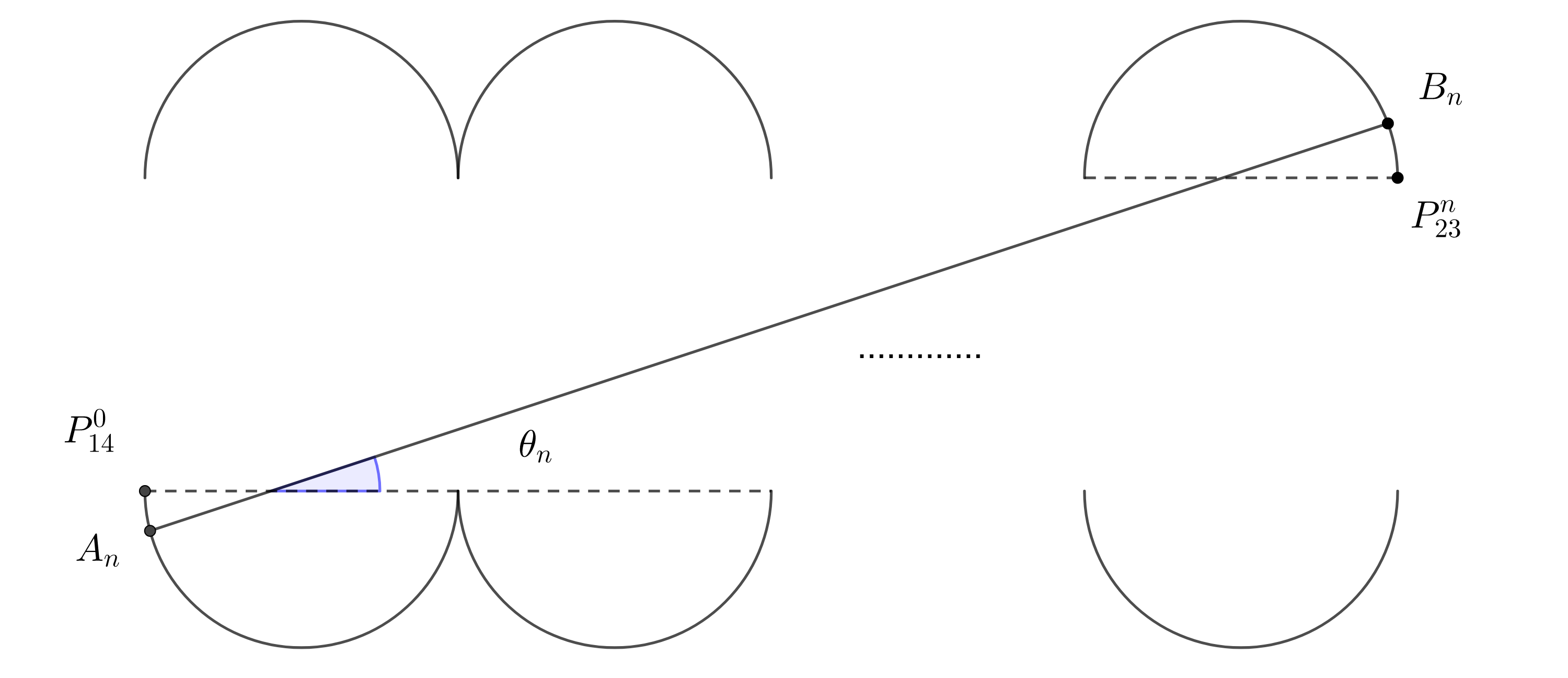
Figure 4: The period two orbit $\overline{\gamma}_{n}$ for the induced billiard map

Proof.

By strict concavity of $\Gamma_{1}^{0}$ and $\Gamma_{2}^{n}$, there is a unique pair of points $A_{n}\in\Gamma_{1}^{0}$ and $B_{n}\in\Gamma_{2}^{n}$, which achieve the maximum of

$$\left\{\left\|\overline{AB}\right\|:\ A\in\Gamma_{1}^{0},\ B\in\Gamma_{2}^{n}\right\}.$$

As a consequence, $\overline{A_{n}B_{n}}$ is perpendicular to $\Gamma_{1}^{0}$ at $A_{n}$, as well as to $\Gamma_{2}^{n}$ at $B_{n}$. Denote the coordinate of $A_{n}$ in $\Gamma_{1}^{0}$ by $\overline{s}_{n}$, and the coordinate of $B_{n}$ in $\Gamma_{2}^{n}$ by $\overline{t}_{n}$, then $\overline{\gamma}_{n}=\overline{A_{n}B_{n}}=\overline{(\overline{s}_{n},0)(\overline{t}_{n},0)}$ is a period two orbit for the induced billiard map on $\Gamma_{1}\cup\Gamma_{2}$.

Recall that $Q$ is the quotient given by (7.1). Let $\theta_{n}$ be the angle formed by the horizontal axis and $\overline{A_{n}B_{n}}$, then as $n\to\infty$,

$$\theta_{n}=\tan\theta_{n}+\mathcal{O}\left(\frac{1}{n^{2}}\right)=\frac{Q}{n}+\mathcal{O}\left(\frac{1}{n^{2}}\right).$$ (7.5)

On the other hand, as $n\to\infty$ and thus $\theta_{n}\to 0$, the point $A_{n}$ is more and more close to $P_{14}^{0}$, and the point $B_{n}$ is more and more close to $P_{23}^{n}$. We approximate $\Gamma_{1}^{0}$ by the osculating circle at $P_{14}^{0}$ with absolute curvature $\mathcal{K}_{14}$, and approximate $\Gamma_{2}^{n}$ by the osculating circle at $P_{23}^{n}$ with absolute curvature $\mathcal{K}_{23}$. Then there exist constants $c_{1},c_{2}\in{\mathbb{R}}$ such that as $n\to\infty$,

$$\theta_{n}=\mathcal{K}_{14}\overline{s}_{n}+c_{1}\overline{s}_{n}^{2}=\mathcal{K}_{23}\overline{t}_{n}+c_{2}\overline{t}_{n}^{2}.$$ (7.6)

Then the estimates in (7.4) directly follows from (7.5) and (7.6). ∎

We also consider periodic billiard trajectories of induced period 4.

Lemma 7.2.

For any fixed $\rho>1$ and any sufficiently large number $n\geq 1$, there exists a period four palindromic trajectory (see Fig. 5)

$$\overline{\gamma}_{n,\rho}=\ \overline{B_{n,\rho}^{\prime}A_{n,\rho}B_{n,\rho}^{\prime\prime}A_{n,\rho}}=\ \overline{(\overline{t}_{n,\rho}^{\prime},0)(\overline{s}_{n,\rho},\overline{\varphi}_{n,\rho})(\overline{t}_{n,\rho}^{\prime\prime},0)(\overline{s}_{n,\rho},-\overline{\varphi}_{n,\rho})},$$

for the induced billiard map on $\Gamma_{1}\cup\Gamma_{2}$, such that $A_{n,\rho}\in\Gamma_{1}^{0}$, $B_{n,\rho}^{\prime}\in\Gamma_{2}^{n}$ and $B_{n,\rho}^{\prime\prime}\in\Gamma_{2}^{\lfloor n\rho\rfloor}$. Moreover, as $n\to\infty$,

$$\begin{split}\overline{t}_{n,\rho}^{\prime}=\frac{Q}{n\mathcal{K}_{23}}+\mathcal{O}\left(\frac{1}{n^{2}}\right),\ \ \ \ \ \ \ \ \ \ &\ \ \ \overline{t}_{n,\rho}^{\prime\prime}=\frac{Q\rho^{-1}}{n\mathcal{K}_{23}}+\mathcal{O}\left(\frac{1}{n^{2}}\right),\\ \overline{s}_{n,\rho}=\frac{Q(1+\rho^{-1})}{2n\mathcal{K}_{14}}+\mathcal{O}\left(\frac{1}{n^{2}}\right),\ \ \ &\ \ \ \overline{\varphi}_{n,\rho}=\frac{Q(1-\rho^{-1})}{2n}+\mathcal{O}\left(\frac{1}{n^{2}}\right).\end{split}$$ (7.7)

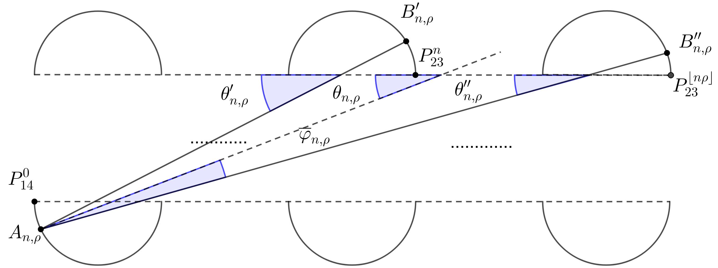
Figure 5: The period four palindromic orbit $\overline{\gamma}_{n,\rho}$ for the induced billiard map

Proof.

Similar to the proof of Lemma 4.1, there exist $A_{n,\rho}\in\Gamma_{1}^{0}$, $B_{n,\rho}^{\prime}\in\Gamma_{2}^{n}$ and $B_{n,\rho}^{\prime\prime}\in\Gamma_{2}^{\lfloor n\rho\rfloor}$, which achieve the maximum of

$$\left\{\left\|\overline{AB^{\prime}}\right\|+\left\|\overline{AB^{\prime\prime}}\right\|:\ A\in\Gamma_{1}^{0},\ B^{\prime}\in\Gamma_{2}^{n},\ B^{\prime\prime}\in\Gamma_{2}^{\lfloor n\rho\rfloor}\right\}.$$

Thus, $\overline{A_{n,\rho}B_{n,\rho}^{\prime}}$ is perpendicular to $\Gamma_{2}^{n}$ at $B_{n,\rho}^{\prime}$, and $\overline{A_{n,\rho}B_{n,\rho}^{\prime\prime}}$ is perpendicular to $\Gamma_{2}^{\lfloor n\rho\rfloor}$ at $B_{n,\rho}^{\prime\prime}$. Moreover, the angle $\angle(\overline{A_{n,\rho}B_{n,\rho}^{\prime}},\mathcal{N})$ is equal to the angle $\angle(\overline{A_{n,\rho}B_{n,\rho}^{\prime\prime}},,\mathcal{N})$, where $\mathcal{N}$ is the inner normal direction of $\Gamma_{1}^{0}$ at $A_{n,\rho}$. We denote this angle by $\overline{\varphi}_{n,\rho}$. We further denote the coordinate of $A_{n,\rho}$ in $\Gamma_{1}^{0}$ by $\overline{s}_{n,\rho}$, the coordinate of $B_{n,\rho}^{\prime}$ in $\Gamma_{2}^{n}$ by $\overline{t}_{n,\rho}^{\prime}$, and the coordinate of $B_{n,\rho}^{\prime\prime}$ in $\Gamma_{2}^{\lfloor n\rho\rfloor}$ by $\overline{t}_{n,\rho}$. Then it is clear that

$$\overline{\gamma}_{n,\rho}=\ \overline{B_{n,\rho}^{\prime}A_{n,\rho}B_{n,\rho}^{\prime\prime}A_{n,\rho}}=\ \overline{(\overline{t}_{n,\rho}^{\prime},0)(\overline{s}_{n,\rho},\overline{\varphi}_{n,\rho})(\overline{t}_{n,\rho}^{\prime\prime},0)(\overline{s}_{n,\rho},-\overline{\varphi}_{n,\rho})},$$

is a period four orbit for the induced billiard map on $\Gamma_{1}\cup\Gamma_{2}$.

Let $\theta_{n,\rho}^{\prime}$, $\theta_{n,\rho}^{\prime\prime}$ and $\theta_{n,\rho}$ be the angles formed by horizontal axis with $\overline{A_{n,\rho}B_{n,\rho}^{\prime}}$, $\overline{A_{n,\rho}B_{n,\rho}^{\prime}}$ and $\mathcal{N}$ respectively. Then we have

$$\overline{\varphi}_{n,\rho}=\theta_{n,\rho}^{\prime}-\theta_{n,\rho}=\theta_{n,\rho}-\theta_{n,\rho}^{\prime\prime}.$$

As $n\to\infty$,

$$\begin{split}\theta_{n,\rho}^{\prime}&=\tan\theta_{n,\rho}^{\prime}+\mathcal{O}\left(\frac{1}{n^{2}}\right)=\frac{Q}{n}+\mathcal{O}\left(\frac{1}{n^{2}}\right),\\ \theta_{n,\rho}^{\prime\prime}&=\tan\theta_{n,\rho}^{\prime\prime}+\mathcal{O}\left(\frac{1}{n^{2}}\right)=\frac{Q\rho^{-1}}{n}+\mathcal{O}\left(\frac{1}{n^{2}}\right),\end{split}$$ (7.8)

which implies that

$$\begin{split}\theta_{n,\rho}&=\frac{\theta_{n,\rho}^{\prime}+\theta_{n,\rho}^{\prime\prime}}{2}=\frac{Q(1+\rho^{-1})}{2n}+\mathcal{O}\left(\frac{1}{n^{2}}\right),\\ \overline{\varphi}_{n,\rho}&=\frac{\theta_{n,\rho}^{\prime}-\theta_{n,\rho}^{\prime\prime}}{2}=\frac{Q(1-\rho^{-1})}{2n}+\mathcal{O}\left(\frac{1}{n^{2}}\right).\end{split}$$ (7.9)

We again approximate $\Gamma_{1}^{0}$ by the osculating circle at $P_{14}^{0}$, approximate $\Gamma_{2}^{n}$ by the osculating circle at $P_{23}^{n}$, and approximate $\Gamma_{2}^{\lfloor n\rho\rfloor}$ by the osculating circle at $P_{23}^{\lfloor n\rho\rfloor}$, then there exist constants $c_{1},c_{2}\in{\mathbb{R}}$ such that

$$\theta_{n,\rho}=\mathcal{K}_{14}\overline{s}_{n,\rho}+c_{1}\overline{s}_{n,\rho}^{2},\ \ \text{and}\ \ \theta_{n,\rho}^{*}=\mathcal{K}_{23}\overline{t}_{n,\rho}^{*}+c_{2}\left(\overline{t}_{n,\rho}^{*}\right)^{2}\ \text{for}\ *=\prime,\ \prime\prime.$$ (7.10)

Then the estimate (7.7) directly follows from (7.8), (7.9) and (7.10). ∎

7.2 Flatness of $\mathbf{n}$ at $P_{14}$ and $P_{23}$

Recall that $\mathbf{n}\equiv 0$ on $J_{3}\cup J_{4}$. We introduce arclength parameter $s$ on $\Gamma_{1}$ such that $P_{14}$ corresponds to $s=0$, and arclength parameter $t$ on $\Gamma_{2}$ such that $P_{23}$ corresponds to $t=0$. Then we rewrite $\mathbf{n}$ as $\mathbf{n}_{1}(s)$ on $\Gamma_{1}$ and by $\mathbf{n}_{2}(t)$ on $\Gamma_{2}$. Note that $\mathbf{n}_{1}(0)=\mathbf{n}_{2}(0)=0$.

Under the assumption that (7.3) holds for the special orbits $\overline{\gamma}_{n}$ and $\overline{\gamma}_{n,\rho}$, we shall prove the flatness of the deformation function $\mathbf{n}$ at the two gluing points $P_{14}$ and $P_{23}$, that is,

Proposition 7.3.

If $\sum_{\overline{\gamma}_{n}}G=\sum_{\overline{\gamma}_{n,\rho}}G=0$ for any $n\geq 1$ and $\rho>1$, then

$$\mathbf{n}_{1}^{(d)}(0)=\mathbf{n}_{2}^{(d)}(0)=0,\ \ \text{for any}\ d\geq 1.$$ (7.11)

Stadium Rigidity Theorem immediately follows from Proposition 7.3, since $\mathbf{n}_{1}$ and $\mathbf{n}_{2}$ are constantly zero as they are both analytic. In the rest of this section, we prove Proposition 7.3.

Proof of Proposition 7.3.

If (7.11) does not hold, we can find a minimal integer $d_{i}\geq 1$ such that $c_{i}:=\mathbf{n}_{i}^{(d_{i})}(0)\neq 0$, $i=1,2$. Recall that $\mathbf{n}_{1}(0)=\mathbf{n}_{2}(0)=0$.

We then further find $u>0$ such that the Taylor expansion is valid for $\mathbf{n}_{1}(s)$ on $s\in[0,u]$ up to order $d_{1}$, and for $\mathbf{n}_{2}(t)$ on $t\in[0,u]$ up to order $d_{2}$. In this way, for any $s,t\in[0,u]$, we write

$$\mathbf{n}_{1}(s)=c_{1}s^{d_{1}}+\mathcal{O}(s^{d_{1}+1}),\ \ \text{and}\ \ \mathbf{n}_{2}(t)=c_{2}t^{d_{2}}+\mathcal{O}(t^{d_{2}+1}).$$ (7.12)

By Lemma 7.1, for sufficiently large $n\geq 1$, there is a period two trajectory $\overline{\gamma}_{n}=\overline{(\overline{s}_{n},0)(\overline{t}_{n},0)}$ for the induced billiard map, such that $\overline{s}_{n},\overline{t}_{n}\in[0,u]$. Then by the assumption $\sum_{\overline{\gamma}_{n}}G=0$, we immediately get

$$\mathbf{n}_{1}(\overline{s}_{n})+\mathbf{n}_{2}(\overline{t}_{n})=0.$$

By (7.4) and (7.12), we obtain

$$c_{1}\left(\frac{Q}{n\mathcal{K}_{14}}\right)^{d_{1}}+c_{2}\left(\frac{Q}{n\mathcal{K}_{23}}\right)^{d_{2}}+\mathcal{O}\left(\frac{1}{n^{\min\{d_{1},d_{2}\}+1}}\right)=0.$$ (7.13)

We claim that $d_{1}=d_{2}$. Otherwise, to fix ideas let us assume that $d_{2}>d_{1}=\min\{d_{1},d_{2}\}$. Multiplying $\left(\frac{Q}{n\mathcal{K}_{14}}\right)^{-d_{1}}$ on both sides of (7.13), and then letting $n\to\infty$, we immediately get $c_{1}=0$, which contradicts our choice of $d_{1}$.

Now we set $d_{1}=d_{2}=d$. We use the same trick again, that is, multiplying $\left(\frac{Q}{n}\right)^{-d}$ on both sides of (7.13), and then letting $n\to\infty$, we get

$$c_{1}\mathcal{K}_{14}^{-d}+c_{2}\mathcal{K}_{23}^{-d}=0.$$ (7.14)

By Lemma 7.2, for any fixed $\rho>1$ and any sufficiently large number $n\geq 1$, there is a period four trajectory

$$\overline{\gamma}_{n,\rho}=\overline{(\overline{t}_{n,\rho}^{\prime},0)(\overline{s}_{n,\rho},\overline{\varphi}_{n,\rho})(\overline{t}_{n,\rho}^{\prime\prime},0)(\overline{s}_{n,\rho},-\overline{\varphi}_{n,\rho})},$$

for the induced billiard map, such that $\overline{s}_{n,\rho},\overline{t}_{n,\rho}^{\prime},\overline{t}_{n,\rho}^{\prime\prime}\in[0,u]$ and the angle $\overline{\varphi}_{n,\rho}$ is very close to zero. By the assumption $\sum_{\overline{\gamma}_{n,\rho}}G=0$, we have

$$2\mathbf{n}_{1}(\overline{s}_{n,\rho})\cos\overline{\varphi}_{n,\rho}+\mathbf{n}_{2}(\overline{t}_{n,\rho}^{\prime})+\mathbf{n}_{2}(\overline{t}_{n,\rho}^{\prime\prime})=0.$$

By (7.7) and (7.12), as well as the fact that $\cos\overline{\varphi}_{n,\rho}=1+\mathcal{O}(\overline{\varphi}_{n,\rho}^{2})=1+\mathcal{O}(n^{-2})$ as $n\to\infty$, we obtain

$$2c_{1}\left(\frac{Q(1+\rho^{-1})}{2n\mathcal{K}_{14}}\right)^{d}+c_{2}\left(\frac{Q}{n\mathcal{K}_{23}}\right)^{d}+c_{2}\left(\frac{Q\rho^{-1}}{n\mathcal{K}_{23}}\right)^{d}+\mathcal{O}\left(\frac{1}{n^{d+1}}\right)=0.$$

Multiplying $\left(\frac{Q}{n}\right)^{-d}$ on both sides of the above, and letting $n\to\infty$, we get

$$c_{1}\cdot 2^{1-d}\mathcal{K}_{14}^{-d}\left(1+\rho^{-1}\right)^{d}+c_{2}\mathcal{K}_{23}^{-d}(1+\rho^{-d})=0.$$ (7.15)

Combining (7.14) and (7.15), we obtain a homogeneous system of linear equations with two variables $c_{1}$ and $c_{2}$, whose coefficient matrix has determinant

$$\det\begin{pmatrix}\mathcal{K}_{14}^{-d}&\mathcal{K}_{23}^{-d}\\ 2^{1-d}\mathcal{K}_{14}^{-d}\left(1+\rho^{-1}\right)^{d}&\mathcal{K}_{23}^{-d}(1+\rho^{-d})\end{pmatrix}=\frac{1+\rho^{-d}-2^{1-d}(1+\rho^{-1})^{d}}{\mathcal{K}_{14}^{d}\mathcal{K}_{23}^{d}}.$$

For any $d\geq 1$, it is easy to pick $\rho>1$ such that the above determinant is non-zero, and hence $c_{1}=c_{2}=0$, which is a contradiction. Therefore, we must have $\mathbf{n}_{1}^{(d)}(0)=\mathbf{n}_{2}^{(d)}(0)=0$ for any $d\geq 1$. ∎

8 Analysis of Periodic Orbits with Rotation Number $\pm\frac{n}{2n+1}$

8.1 Periodic Orbits with Rotation Number $\pm\frac{n}{2n+1}$

Let $\Omega$ be a Bunimovich squash-type stadium in $\mathcal{M}^{m}_{ss}$ for $m\geq 3$. We introduce all the possible periodic $(2n+1)$ orbits whose rotation number is either $\frac{n}{2n+1}$ or $-\frac{n}{2n+1}$. More precisely, for any integer $n\geq 1$, we consider the periodic orbit $\gamma_{n}^{i}$ associated with the symbolic code

$$(i\underbrace{12\cdots 12}_{2n}),$$ (8.1)

for $i=1,2,3,4$. The existence and uniqueness of the orbit $\gamma_{n}^{i}$ can be proven in a similar fashion as in Lemma 4.1, that is,

• the orbit $\gamma^{1}_{n}$ is the unique global maximum point of the length function

  $$L(r_{0},r_{1},\dots,r_{2n})=\sum_{k=0}^{2n}\tau(r_{k},r_{k+1}),\ \ \text{with}\ r_{2n+1}=r_{0},$$

  for $(r_{0},r_{1},\dots,r_{2n})\in\Gamma_{1}\times(\Gamma_{1}\times\Gamma_{2})^{n}$ with the restriction that $r_{0}\geq 0\geq r_{1}$. Such restriction makes $r_{0}$ and $r_{1}$ fall in different sides of $x$. Similarly, $\gamma^{2}_{n}$ is the global maximum point of the same length function but for $(r_{0},r_{1},\dots,r_{2n})\in\Gamma_{2}\times(\Gamma_{1}\times\Gamma_{2})^{n}$ with the restriction that $r_{0}\geq 0\geq r_{2n}$.

• the orbit $\gamma^{3}_{n}$ corresponds to unfolded orbit $\widetilde{\gamma}^{3}_{n}$, which is the unique global maximum point of the length function on the double cover table $\widetilde{\Omega}$ (see Fig. 1, right, which has a symmetric reflection line through $\Gamma_{3}$), given by

  $$L(r_{0},r_{1},\dots,r_{2n})=\sum_{k=0}^{2n-1}\widetilde{\tau}(r_{k},r_{k+1})$$

  for $(r_{0},r_{1},\dots,r_{2n})\in\widetilde{\Gamma}_{2}\times(\Gamma_{1}\times\Gamma_{2})^{n}$ with the restriction that $r_{0}^{*}=r_{2n}$, where $r_{0}^{*}\in\Gamma_{2}$ denotes the reflected point of $r_{0}\in\widetilde{\Gamma}_{2}$ by the symmetry line through $\Gamma_{3}$. The orbit $\gamma^{4}_{n}$ can be obtained in a similar fashion by considering the double cover table with symmetry line through $\Gamma_{4}$.

As the winding number of a periodic orbit is counted in the counter-clockwise direction, the rotation number of $\gamma_{n}^{i}$ equals to $(-1)^{i}\frac{n}{2n+1}$ for $i=1,2,3,4$. Switching the roles of $\Gamma_{1}$ and $\Gamma_{2}$, we could also consider the periodic orbit $\widehat{\gamma}_{n}^{i}$ associated with

$$(i\underbrace{21\cdots 21}_{2n}).$$

It is easy to see that $\widehat{\gamma}_{n}^{i}$ is the inverse orbit of $\gamma_{n}^{i}$. Therefore, $\widehat{\gamma}_{n}^{i}$ and $\gamma_{n}^{i}$ are of the same total length, and the rotation number of $\widehat{\gamma}_{n}^{i}$ equals to $(-1)^{i+1}\frac{n}{2n+1}$.

Along any of the above orbits, i.e., $\gamma^{i}_{n}$ and $\widehat{\gamma}^{i}_{n}$ with $i=1,2,3,4$, a billiard ball moves from an initial position on $\Gamma_{i}$, collides successively between $\Gamma_{1}$ and $\Gamma_{2}$ for $2n$ times, and then gets back to the initial position on $\Gamma_{i}$. It is easy to see that the first $n$ collisions approach the period two orbit $\gamma^{*}$, while the last $n$ collisions become away from $\gamma^{*}$. There are essentially two types:

• $\gamma^{i}_{n}$ and $\widehat{\gamma}^{i}_{n}$ are symmetric for $i=3,4$, i.e., the number of times that the billiard ball lies on $\Gamma_{1}$ is the same as that on $\Gamma_{2}$ in one period;

• $\gamma^{i}_{n}$ and $\widehat{\gamma}^{i}_{n}$ are asymmetric for $i=1,2$, i.e., the number of times that the billiard ball lies on $\Gamma_{1}$ is different from that on $\Gamma_{2}$ in one period.

It turns out that the trace of the above periodic orbits in the same type are similar. To illustrate the corresponding dynamics, we picture the following two sequence of periodic orbits $\gamma_{n}^{2}$ and $\gamma_{n}^{3}$. Recall that the period two orbit is denoted by $\gamma^{*}=\overline{AB}$. Along the asymmetric orbit $\gamma_{n}^{2}$ (see Fig. 6, upper), a billiard ball lies on the closest position near $A$ (or $B$) at the $n$-th and near $B$ (or $A$) at the $(n+1)$-th collision if $n$ is odd (if $n$ is even); along the symmetric orbit $\gamma_{n}^{3}$ (see Fig. 6, lower), every free path crosses $\overline{AB}$ except the middle path from the $n$-th collision to the $(n+1)$-th collision.

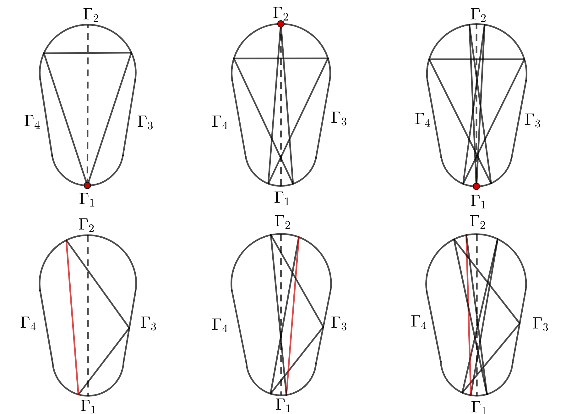
Figure 6: Upper: $\gamma_{n}^{2}$ with $n=1,2,3$;  Lower: $\gamma_{n}^{3}$ with $n=1,2,3$.

8.2 The Homoclinic Semi-orbits and the Shadowing Estimates

For $i=1,2,3$ or $4$, we denote the collision points of $\gamma_{n}^{i}$ by

$$y^{i}_{n}(0)\mapsto x^{i}_{n}(1)\mapsto y^{i}_{n}(1)\mapsto\dots\mapsto x^{i}_{n}(n)\mapsto y^{i}_{n}(n),$$

where

• at the initial stage, we denote by $y^{i}_{n}(0)=(t^{i}_{n}(0),\psi^{i}_{n}(0))$ the collision point on $\Gamma_{i}$;

• at the stage of $2n$ successive collisions between $\Gamma_{1}$ and $\Gamma_{2}$, we denote

  $$\text{on}\ \Gamma_{1}:\ x^{i}_{n}(k) =(s^{i}_{n}(k),\varphi^{i}_{n}(k)),\ k=1,2,\dots,n;$$

  $$\text{on}\ \Gamma_{2}:\ y^{i}_{n}(k) =(t^{i}_{n}(k),\psi^{i}_{n}(k)),\ k=1,2,\dots,n.$$

Similarly, we denote the collision points of the inverse orbit $\widehat{\gamma}_{n}^{i}$ by

$$\widehat{x}^{i}_{n}(0)\mapsto\widehat{y}^{i}_{n}(1)\mapsto\widehat{x}^{i}_{n}(1)\mapsto\dots\mapsto\widehat{y}^{i}_{n}(n)\mapsto\widehat{x}^{i}_{n}(n),$$

with coordinates $\widehat{x}^{i}_{n}(k)=(\widehat{s}^{i}_{n}(k),\widehat{\varphi}^{i}_{n}(k))$ for $k=0,1,\dots,n$ and $\widehat{y}^{i}_{n}(k)=(\widehat{t}^{i}_{n}(k),\widehat{\psi}^{i}_{n}(k))$ for $k=1,\dots,n$. Unlike the palindromic orbits $\gamma_{n}$, the time reversibility does not hold for $\gamma^{i}_{n}$ or $\widehat{\gamma}_{n}^{i}$ itself, but $\gamma_{n}^{i}$ and $\widehat{\gamma}_{n}^{i}$ form an involution pair, that is,

$$\begin{split}\widehat{s}_{n}^{i}(n+1-k)=s_{n}^{i}(k),\ \widehat{\varphi}_{n}^{i}(n+1-k)=-\varphi_{n}^{i}(k),\ k=1,2,\dots,n,\\ \widehat{t}_{n}^{i}(n+1-k)=t_{n}^{i}(k),\ \widehat{\psi}_{n}^{i}(n+1-k)=-\psi_{n}^{i}(k),\ k=1,2,\dots,n.\end{split}$$ (8.2)

Also, $\widehat{s}_{n}^{i}(0)=t_{n}^{i}(0)$ and $\widehat{\varphi}_{n}^{i}(0)=-\psi_{n}^{i}(0)$.

Using similar arguments as in Lemma 4.2 and Lemma 4.3, we can define a homoclinic semi-orbit of the period two orbit $\gamma^{*}=\overline{xy}$ by

$$\gamma^{i}_{\infty}:=(x^{i}_{\infty}(0)\ x^{i}_{\infty}(1)\ y^{i}_{\infty}(1)\ x^{i}_{\infty}(2)\ y^{i}_{\infty}(2)\dots),$$

which corresponds to the symbolic code $(i1212\cdots)$, where

$$\begin{split}x^{i}_{\infty}(k)&=\lim_{n\to\infty}x^{i}_{n}(k),\ k=1,2,\dots;\\ y^{i}_{\infty}(k)&=\lim_{n\to\infty}y^{i}_{n}(k),\ k=0,1,2,\dots.\end{split}$$

We write the coordinates $x^{i}_{\infty}(k)=(s^{i}_{\infty}(k),\varphi^{i}_{\infty}(k))$ for $k=1,2,\dots$, and $y^{i}_{\infty}(k)=(t^{i}_{\infty}(k),\psi^{i}_{\infty}(k))$ for $k=0,1,2,\dots$.

Similar to Lemma 4.4 and Lemma 4.6, we can provide estimates for the convergence of $\gamma^{i}_{\infty}$ to $\gamma^{*}$, and for the shadowing of $\gamma^{i}_{n}$ along $\gamma^{i}_{\infty}$ as follows.

Lemma 8.1.

Let $i=1,2,3$ or $4$.

• The following estimates hold for the homoclinic orbit $\gamma_{\infty}^{i}$:

  $$\begin{split}x^{i}_{\infty}(k)=\lambda^{-k}(C_{s}^{i},C_{\varphi}^{i})+\mathcal{O}(\lambda^{-1.5k}),&\ \ k=1,2,\dots,\\ y^{i}_{\infty}(k)=\lambda^{-k}(C_{t}^{i},C_{\psi}^{i})+\mathcal{O}(\lambda^{-1.5k}),&\ \ k=0,1,2,\dots,\end{split}$$ (8.3)

  where the constants $C^{i}_{s},C^{i}_{\varphi},C^{i}_{t}$ and $C_{\psi}^{i}$ satisfy the following relation:

  $$\dfrac{C_{\varphi}^{i}}{C_{s}^{i}}=\frac{\lambda^{-1}-\lambda}{4a_{2}\tau^{*}},\ \ \dfrac{C_{\psi}^{i}}{C_{t}^{i}}=\frac{\lambda^{-1}-\lambda}{4a_{1}\tau^{*}},\ \ \text{and}\ \ \dfrac{C_{t}^{i}}{C_{s}^{i}}=-\frac{1+\lambda^{-1}}{2a_{2}}=-\frac{2a_{1}}{1+\lambda}.$$ (8.4)

• The following estimates hold for the periodic orbit $\gamma_{n}^{i}$:

  $$\begin{split}x^{i}_{n}(k)-x^{i}_{\infty}(k)=\lambda^{k-n}(C^{i}_{s,k},C^{i}_{\varphi,k})+\mathcal{O}(\lambda^{0.5k-n}),&\ \ k=1,\dots,\left\lfloor\frac{n}{2}\right\rfloor+1,\\ y^{i}_{n}(k)-y^{i}_{\infty}(k)=\lambda^{k-n}(C^{i}_{t,k},C^{i}_{\psi,k})+\mathcal{O}(\lambda^{0.5k-n}),&\ \ k=0,1,\dots,\left\lfloor\frac{n}{2}\right\rfloor+1.\end{split}$$ (8.5)

  where the constants $C^{i}_{s,k},C^{i}_{\varphi,k},C^{i}_{t,k}$ and $C^{i}_{\psi,k}$ are given by

  $$\begin{split}C^{i}_{s,k}=C_{s}^{i}\lambda^{-1}(\lambda^{-2k}+\Theta_{i}),\ \ &\ \ C^{i}_{\varphi,k}=C^{i}_{\varphi}\lambda^{-1}(\lambda^{-2k}-\Theta_{i}),\\ C^{i}_{t,k}=C^{i}_{t}\lambda^{-1}(\lambda^{-2k}+\Theta_{i}),\ \ &\ \ C^{i}_{\psi,k}=C^{i}_{\psi}\lambda^{-1}(\lambda^{-2k}-\Theta_{i}).\end{split}$$ (8.6)

  Here $\Theta_{i}=-1$ if $i=1,2$, and $\Theta_{3}=\dfrac{\tan\theta_{1}+\mathcal{K}_{A}}{\tan\theta_{1}-\mathcal{K}_{A}}$, $\Theta_{4}=\dfrac{\tan\theta_{2}+\mathcal{K}_{B}}{\tan\theta_{2}-\mathcal{K}_{B}}$.

• Alternatively, the following estimates hold for the periodic orbit $\gamma_{n}^{i}$:

  $$\begin{split}x^{i}_{n}(k)-x^{i}_{\infty}(k)=\lambda^{k-n}\left[v^{i}_{\infty}(2k)+o(1)\right],\ \ \ \ \ \ &\ \ k=1,\dots,\left\lfloor{\frac{n}{2}}\right\rfloor+1,\\ y^{i}_{n}(k)-y^{i}_{\infty}(k)=\lambda^{k-n}\left[v^{i}_{\infty}(2k+1)+o(1)\right],\ &\ \ k=0,1,\dots,\left\lfloor{\frac{n}{2}}\right\rfloor+1,\end{split}$$ (8.7)

  where the vectors $v^{i}_{\infty}(m)\in{\mathbb{R}}^{2}$, $m=0^{\pm},0,1,2,\dots$, has uniformly bounded magnitudes.

The proof of Lemma 8.1 is similar to that of Lemma 4.4 and Lemma 4.6, and thus we leave it to the reader. The only difference between the proofs of Lemma 4.4 and Lemma 8.1 is on how to obtain the constant $\Theta_{i}$. That is, in Lemma 4.4 we obtain $\Theta=1$ using the self time-reversibility for the palindromic orbit $\gamma_{n}$, while in Lemma 8.1 we obtain the value of $\Theta_{i}$ by the fact that

• the middle collision point is close to $\gamma^{*}$ for $i=1,2$;

• the middle free path is almost parallel to $\gamma^{*}$ for $i=3,4$.

Similar to Lemma 8.1, corresponding estimates also hold for the inverse periodic orbit $\widehat{\gamma}^{i}_{n}$ and the corresponding homoclinic semi-orbit $\widehat{\gamma}^{i}_{\infty}$, where we simply put ‘hat’ on each term, i.e., $\widehat{x}^{i}_{n}$, $\widehat{x}^{i}_{\infty}$, $\widehat{C}^{i}_{s}$, $\widehat{\Theta}_{i}$, etc. By the above facts (i) and (ii), we shall have

$$\begin{split}&(\widehat{C}^{i}_{s},\widehat{C}^{i}_{\varphi})=(-C^{i}_{s},C^{i}_{\varphi})\ \text{and}\ (\widehat{C}^{i}_{t},\widehat{C}^{i}_{\psi})=(-C^{i}_{t},C^{i}_{\psi})\ \ \text{if}\ i=1,2;\\ &(\widehat{C}^{i}_{s},\widehat{C}^{i}_{\varphi})=(C^{i}_{s},-C^{i}_{\varphi})\ \text{and}\ (\widehat{C}^{i}_{t},\widehat{C}^{i}_{\psi})=(C^{i}_{t},-C^{i}_{\psi})\ \ \text{if}\ i=3,4.\end{split}$$ (8.8)

9 Proof of Theorem 3

9.1 The Length Growth of the Homoclinic Semi-orbit $\gamma_{\infty}^{i}$

In this subsection, we show that for $i=1,2,3$ or $4$, the length growth of the homoclinic semi-orbit $\gamma_{\infty}^{i}$ is exponentially asymptotic to that of the period two orbit $\gamma^{*}$. More precisely, we denote $l_{\infty}^{i}(0)=\tau(t_{\infty}^{i}(0),s_{\infty}^{i}(1))$ and

$$l_{\infty}^{i}(k)=\tau(s_{\infty}^{i}(k),t_{\infty}^{i}(k))+\tau(t_{\infty}^{i}(k),s_{\infty}^{i}(k+1))\ \ \text{for any}\ k\geq 1.$$ (9.1)

Lemma 9.1.

There exists a constant $\mathcal{Q}_{\infty}^{i}\in{\mathbb{R}}$ such that

$$l^{i}_{\infty}(k)-2\tau^{*}=\mathcal{Q}_{\infty}^{i}\lambda^{-2k}+\mathcal{O}\left(\lambda^{-2.5k}\right).$$ (9.2)

Proof.

Note that $\tau(s_{\infty}^{i}(k),t_{\infty}^{i}(k))-\tau^{*}$ is the difference of the free path travelled by moving from $(s,t)=(0,0)$ to

$$(s,t)=(s_{\infty}^{i}(k),t_{\infty}^{i}(k))=\lambda^{-k}(C_{s}^{i},C_{t}^{i})+\mathcal{O}(\lambda^{-1.5k}),$$

where the estimates are due to Lemma 8.1. By (3.4),

$$\tau(s_{\infty}^{i}(k),t_{\infty}^{i}(k))-\tau^{*}$$

$$= \frac{1}{2\tau^{*}}\left[a_{1}\left(s_{\infty}^{i}(k)\right)^{2}+2s_{\infty}^{i}(k)t^{i}_{\infty}(k)+a_{2}\left(t^{i}_{\infty}(k)\right)^{2}\right]+\mathcal{O}\left(\left(\left(s^{i}_{\infty}(k)\right)^{2}+\left(t^{i}_{\infty}(k)\right)^{2}\right)^{\frac{3}{2}}\right)$$

$$= \dfrac{a_{1}\left(C_{s}^{i}\right)^{2}+2C_{s}^{i}C_{t}^{i}+a_{2}\left(C_{t}^{i}\right)^{2}}{2\tau^{*}}\cdot\lambda^{-2k}+\mathcal{O}\left(\lambda^{-2.5k}\right)=:\mathcal{Q}(C_{s}^{i},C_{t}^{i})\cdot\lambda^{-2k}+\mathcal{O}\left(\lambda^{-2.5k}\right),$$

where $\mathcal{Q}(X,Y)$ is a quadratic form defined by

$$\mathcal{Q}(X,Y)=\dfrac{a_{1}X^{2}+2XY+a_{1}Y^{2}}{2\tau^{*}}.$$ (9.3)

In a similar fashion, we also get

$$\tau(t_{\infty}^{i}(k),s_{\infty}^{i}(k+1))-\tau^{*}=\mathcal{Q}(\lambda^{-1}C_{s}^{i},C_{t}^{i})\cdot\lambda^{-2k}+\mathcal{O}\left(\lambda^{-2.5k}\right).$$

Hence (9.2) is proven if we set $\mathcal{Q}_{\infty}^{i}:=\mathcal{Q}(C_{s}^{i},C_{t}^{i})+\mathcal{Q}(\lambda^{-1}C_{s}^{i},C_{t}^{i}).$ ∎

Similarly, we denote by $\widehat{\gamma}_{\infty}^{i}=(\widehat{x}^{i}_{n}(0)\widehat{y}^{i}_{n}(1)\widehat{x}^{i}_{n}(1)\dots)$ the homoclinic semi-orbit obtained by the limit of the inverse periodic orbits $\widehat{\gamma}_{n}^{i}$. Set $\hat{l}_{\infty}^{i}(0)=\tau(\hat{s}_{\infty}^{i}(0),\hat{t}_{\infty}^{i}(1))$ and

$$\hat{l}_{\infty}^{i}(k)=\tau(\hat{t}_{\infty}^{i}(k),\hat{s}_{\infty}^{i}(k))+\tau(\hat{s}_{\infty}^{i}(k),\hat{t}_{\infty}^{i}(k+1))\ \ \text{for any}\ k\geq 1.$$ (9.4)

Similar to Lemma 9.1, there exists a constant $\widehat{\mathcal{Q}}_{\infty}^{i}\in{\mathbb{R}}$ such that

$$\hat{l}^{\,i}_{\infty}(k)-2\tau^{*}=\widehat{\mathcal{Q}}_{\infty}^{i}\lambda^{-2k}+\mathcal{O}\left(\lambda^{-2.5k}\right).$$ (9.5)

Now we define $B^{i}=B^{i}_{0}+B^{i}_{+}+B^{i}_{-}$, where

$$B^{i}_{0}=2\tau^{*}-l^{i}_{\infty}(0)-\hat{l}^{\,i}_{\infty}(0),\ \ B^{i}_{+}=\sum_{k=1}^{\infty}\left(2\tau^{*}-l^{i}_{\infty}(k)\right),\ \ B^{i}_{-}=\sum_{k=1}^{\infty}\left(2\tau^{*}-\hat{l}^{\,i}_{\infty}(k)\right).$$ (9.6)

9.2 The Length Difference between $\gamma_{n}^{i}$ and $\gamma_{\infty}^{i}$

For the periodic orbit $\gamma_{n}^{i}$, we denote $l_{n}^{i}(0)=\tau(t_{n}^{i}(0),s_{n}^{i}(1))$ and

$$l_{n}^{i}(k)=\tau(s_{n}^{i}(k),t_{n}^{i}(k))+\tau(t_{n}^{i}(k),s_{n}^{i}(k+1))\ \ \text{for any}\ 1\leq k\leq n.$$ (9.7)

Similarly, for the inverse periodic orbit $\widehat{\gamma}_{n}^{i}$, we denote $\hat{l}_{n}^{i}(0)=\tau(\hat{s}_{n}^{i}(0),\hat{t}_{n}^{i}(1))$ and

$$\hat{l}_{n}^{i}(k)=\tau(\hat{t}_{n}^{i}(k),\hat{s}_{n}^{i}(k))+\tau(\hat{s}_{n}^{i}(k),\hat{t}_{n}^{i}(k+1))\ \ \text{for any}\ 1\leq k\leq n.$$ (9.8)

We shall compare the length difference between $(\gamma_{n}^{i}$, $\widehat{\gamma}_{n}^{i})$ and $(\gamma_{\infty}^{i}$, $\widehat{\gamma}_{\infty}^{i})$. More precisely, we set $\ell=\lfloor n/2\rfloor$, $\ell^{\prime}=n-1-\ell$. The total length of $\gamma_{n}^{i}$ (and $\widehat{\gamma}_{n}^{i}$) is given by

$$L\left(\gamma_{n}^{i}\right)=L\left(\widehat{\gamma}_{n}^{i}\right)=\sum_{k=0}^{\ell}l_{n}^{i}(k)+\sum_{k=0}^{\ell^{\prime}}\hat{l}_{n}^{i}(k)+\tau\left(s^{i}_{n}(\ell+1),\hat{t}^{i}_{n}(\ell^{\prime}+1)\right),$$ (9.9)

in which we notice that $\hat{t}^{i}_{n}(\ell^{\prime}+1)=t_{n}^{i}(\ell+1)$. Correspondingly, we define

$$L_{\infty}^{i}(n)=\sum_{k=0}^{\ell}l_{\infty}^{i}(k)+\sum_{k=0}^{\ell^{\prime}}\hat{l}_{\infty}^{i}(k)+\tau\left(s^{i}_{\infty}(\ell+1),\hat{t}^{i}_{\infty}(\ell^{\prime}+1)\right),$$ (9.10)

where $l_{\infty}^{i}(k)$ and $\hat{l}_{\infty}^{i}(k)$ are given by (9.1) and (9.4) respectively.

Lemma 9.2.

There exists a constant $\mathcal{C}_{\infty}^{i}\in{\mathbb{R}}$ such that

$$L\left(\gamma_{n}^{i}\right)-L_{\infty}^{i}(n)=\mathcal{C}_{\infty}^{i}\lambda^{-n}+\mathcal{O}\left(\lambda^{-1.5n}\right).$$ (9.11)

Proof.

By Lemma 2.1 and Lemma 8.1, for any $k=0,1,\dots,\ell+1$, we can write

$$\tau(s_{n}^{i}(k),t_{n}^{i}(k))-\tau(s_{\infty}^{i}(k),t_{\infty}^{i}(k))=I_{k}^{0}+J_{k}^{0}+\mathcal{O}\left(\lambda^{-1.5n}\right),$$

where

$$I_{k}^{0} = -\sin\varphi^{i}_{\infty}(k)\ (s_{n}^{i}(k)-s^{i}_{\infty}(k))+\sin\psi^{i}_{\infty}(k)\ (t_{n}^{i}(k)-t_{\infty}^{i}(k)),$$

$$J_{k}^{0} = \frac{1}{2\tau(s^{i}_{\infty}(k),t^{i}_{\infty}(k))}\left[\alpha(s^{i}_{\infty}(k))(s_{n}^{i}(k)-s^{i}_{\infty}(k))^{2}+\alpha(t^{i}_{\infty}(k))(t^{i}_{n}(k)-t^{i}_{\infty}(k))^{2}\right.$$

$$\ \ \ \ \ \ \ \ \ \ \ \ \ \ \ \ \ \ \left.+2\cos\varphi^{i}_{\infty}(k)\cos\psi^{i}_{\infty}(k)(s_{n}^{i}(k)-s^{i}_{\infty}(k))(t^{i}_{n}(k)-t^{i}_{\infty}(k))\right].$$

In a similar fashion, we can write

$$\begin{split}&\tau(t_{n}^{i}(k),s_{n}^{i}(k+1))-\tau(t_{\infty}^{i}(k),s_{\infty}^{i}(k+1))=I_{k}^{1}+J_{k}^{1}+\mathcal{O}\left(\lambda^{-1.5n}\right),\\ &\tau(\hat{t}_{n}^{\,i}(k),\hat{s}_{n}^{\,i}(k),)-\tau(\hat{t}_{\infty}^{\,i}(k),\hat{s}_{\infty}^{\,i}(k))=I_{k}^{2}+J_{k}^{2}+\mathcal{O}\left(\lambda^{-1.5n}\right),\\ &\tau(\hat{s}_{n}^{\,i}(k),\hat{t}_{n}^{\,i}(k+1))-\tau(\hat{s}_{\infty}^{\,i}(k),\hat{t}_{\infty}^{\,i}(k+1))=I_{k}^{3}+J_{k}^{3}+\mathcal{O}\left(\lambda^{-1.5n}\right),\end{split}$$

where $I_{k}^{j}$ (resp. $J_{k}^{j}$), $j=1,2,3$, are of similar form as $I_{k}^{0}$ (resp. $J_{k}^{0}$). Also,

$$\tau\left(s^{i}_{\infty}(\ell+1),\hat{t}^{i}_{\infty}(\ell^{\prime}+1)\right)-\tau\left(s^{i}_{\infty}(\ell+1),\hat{t}^{i}_{\infty}(\ell^{\prime}+1)\right)=I_{*}+J_{*}+\mathcal{O}\left(\lambda^{-1.5n}\right).$$

Therefore,

$$L\left(\gamma_{n}^{i}\right)-L_{\infty}^{i}(n)=I+J+\mathcal{O}\left(\lambda^{-1.5n}\right),$$

where the linear order summation $I$ is an telescopic sum, i.e.,

$$\begin{split}I&:=\sum_{k=0}^{\ell}(I^{0}_{k}+I^{1}_{k})+\sum_{k=0}^{\ell^{\prime}}(I^{2}_{k}+I^{3}_{k})+I_{*}\\ &=-\sin\varphi_{\infty}^{i}(\ell+1)s^{i}_{\infty}(\ell+1)-\sin\widehat{\varphi}_{\infty}^{\,i}(\ell+1)\hat{s}^{i}_{\infty}(\ell+1)=\mathcal{O}\left(\lambda^{-1.5n}\right),\end{split}$$

where the error estimate is due to Lemma 8.1, Part (a) and (8.8). Now we focus on the computation of the second order summation $J$, and by Lemma 8.1, Part (c), we have

$$J:=\sum_{k=0}^{\ell}(J^{0}_{k}+J^{1}_{k})+\sum_{k=0}^{\ell^{\prime}}(J^{2}_{k}+I^{3}_{k})+J_{*}=\sum_{k=\lfloor\ell/2\rfloor}^{\ell}(J^{0}_{k}+J^{1}_{k})+\sum_{k=\lfloor\ell/2\rfloor}^{\ell^{\prime}}(J^{2}_{k}+I^{3}_{k})+J_{*}+\mathcal{O}\left(\lambda^{-1.5n}\right).$$

For any $k\in[\ell/2,\ell]$, by Lemma 8.1, Part (a) again, we have

$$\cos\varphi^{i}_{\infty}(k)\approx 1,\ \ \cos\psi^{i}_{\infty}(k)\approx 1,\ \ \alpha(s^{i}_{\infty}(k))\approx a_{1},\ \ \alpha(s^{i}_{\infty}(k))\approx a_{2},\ \ \tau(s^{i}_{\infty}(k),t^{i}_{\infty}(k))\approx\tau^{*},$$

up to errors of order $\mathcal{O}(\lambda^{-2k})$. By Lemma 8.1, Part (b), we have

$$|s_{n}^{i}(k)-s_{\infty}^{i}(k)|\approx C_{s}^{i}\Theta_{i}\lambda^{k-n-1},\ \ |t_{n}^{i}(k)-t_{\infty}^{i}(k)|\approx C_{t}^{i}\Theta_{i}\lambda^{k-n-1}.$$

up to errors of order $\mathcal{O}(\lambda^{0.5k-n-1})$. Therefore, we have

$$J_{k}^{0}=\Theta_{i}^{2}\mathcal{Q}(C_{s}^{i},C_{t}^{i})\cdot\lambda^{2(k-n-1)}+\mathcal{O}\left(\lambda^{2(0.5k-n-1)}\right),$$

where $\mathcal{Q}(\cdot,\cdot)$ is the quadratic form $\mathcal{Q}(\cdot,\cdot)$ defined in (9.3). Hence

$$\sum_{k=0}^{\ell}J^{0}_{k}=\sum_{k=\lfloor\ell/2\rfloor}^{\ell}J^{0}_{k}+\mathcal{O}\left(\lambda^{-1.5n}\right)=\mathcal{C}_{\infty,0}^{i}\lambda^{-n}+\mathcal{O}\left(\lambda^{-1.5n}\right),$$

where we set $\mathcal{C}^{i}_{\infty,0}:=\begin{cases}\Theta_{i}^{2}\mathcal{Q}(C_{s}^{i},C_{t}^{i})/(\lambda^{2}-1),\ &\text{if}\ n=2\ell,\\ \lambda^{-1}\Theta_{i}^{2}\mathcal{Q}(C_{s}^{i},C_{t}^{i})/(\lambda^{2}-1),\ &\text{if}\ n=2\ell+1.\end{cases}$ In a similar fashion, we can show that there are constants $\mathcal{C}^{i}_{\infty,j}$, $j=1,2,3,*$, such that sums of $J^{j}_{k}$, $j=1,2,3$, and $J_{*}$ satisfy similar estimates as in (9.2). Hence (9.11) holds if we take $\mathcal{C}^{i}_{\infty}=\sum_{j=0}^{3}\mathcal{C}^{i}_{\infty,j}+\mathcal{C}^{i}_{\infty,*}$. ∎

9.3 Proof of Theorem 3

Recall the definitions of $B_{i}$ and $L_{\infty}^{i}(n)$ in (9.6) and (9.10) respectively. Note that

$$\begin{split}&L_{\infty}^{i}(n)-(2n+1)\tau^{*}+B_{i}\\ =&\sum_{k>\ell}\left(l^{i}_{\infty}(k)-2\tau^{*}\right)+\sum_{k>\ell^{\prime}}\left(\hat{l}^{\,i}_{\infty}(k)-2\tau^{*}\right)+\left[\tau\left(s^{i}_{\infty}(\ell+1),\hat{t}^{i}_{\infty}(\ell^{\prime}+1)\right)-\tau^{*}\right].\end{split}$$

Recall that $\ell=\lfloor n/2\rfloor$ and $\ell^{\prime}=n-1-\ell$. By Lemma (9.10) and also apply its proof to the last term in the above, it is easy to show that there is a constant $\mathcal{E}^{i}_{\infty}$ such that

$$L_{\infty}^{i}(n)-(2n+1)\tau^{*}+B_{i}=\mathcal{E}^{i}_{\infty}\lambda^{-n}+\mathcal{O}\left(\lambda^{-1.5n}\right).$$

By Lemma 9.2, we set $\mathcal{D}_{i}=\mathcal{C}^{i}_{\infty}+\mathcal{E}^{i}_{\infty}$, then

$$L\left(\gamma^{i}_{n}\right)-(2n+1)\tau^{*}+B_{i}=\mathcal{D}_{i}\lambda^{-n}+\mathcal{O}\left(\lambda^{-1.5n}\right).$$

Now we choose $j\in\{1,2,3,4\}$ such that $B_{j}>B_{i}$ for all $i\neq j$. If it happens that $B_{j}=B_{i}$ for distinct $j,i$, we pick $j$ such that $D_{j}>D_{i}$. By such choice, we have

$$\mathcal{ML}^{\max}_{\Omega}\left(\frac{2n}{2n+1}\right)=L\left(\gamma^{j}_{n}\right)$$

for sufficiently large $n$. Then the proof of Theorem 3 is complete if we set $B_{\frac{1}{2}}=B_{j}$ and $D_{\frac{1}{2}}=B_{j}$.

References

- [1] Peter Balint, Jacopo de Simoi, Vadim Kaloshin, and Martin Leguil. Marked Length Spectrum, homoclinic orbits and the geometry of open dispersing billiards. Communications in Mathematical Physics volume 374, 1531–1575 (2020).
- [2] Jesus Carnicer. Weighted interpolation for equidistant nodes. Numer. Algorithms 55 (2010), no. 2-3, 223–232.
- [3] Jianyu Chen, Fang Wang, Hong-Kun Zhang. Markov partition and Thermodynamic Formalism for Hyperbolic Systems with Singularities. Preprint, 49pp, 2017.
- [4] Nikolai Chernov and Roberto Markarian. Chaotic billiards, volume 127 of Mathematical Surveys and Monographs. American Mathematical Society, Providence, RI, 2006.
- [5] Colin de Verdière, Y. Sur les longueurs des trajectoires périodiques d’un billard. South Rhone seminar on geometry, III (Lyon, 1983), 122–139, Travaux en Cours, Hermann, Paris, 1984.
- [6] Christopher B. Croke. Rigidity for surfaces of nonpositive curvature. Comment. Math. Helv., 65(1):150–169, 1990.
- [7] Christopher B. Croke and Vladimir A. Sharafutdinov. Spectral rigidity of a compact negatively curved manifold. Topology 37 (1998), no. 6, 1265–1273.
- [8] Jacopo de Simoi, Vadim Kaloshin, and Martin Leguil. Marked Length Spectral determination of analytic chaotic billiards with axial symmetries. Preprint, 57pp, 2019.
- [9] Jacopo de Simoi, Vadim Kaloshin, and Qiaoling Wei. Dynamical spectral rigidity among Z2-symmetric strictly convex domains close to a circle. Ann. of Math. (2), 186(1):277–314, 2017. Appendix B coauthored with H. Hezari.
- [10] C. Gordon, D. L. Webb, and S. Wolpert. One cannot hear the shape of a drum, Bull. Amer. Math. Soc. 27(1992), 134–138.
- [11] Colin Guillarmou and Thibault Lefeuvre. The marked length spectrum of Anosov manifolds. Ann. of Math. (2) 190 (2019), no. 1, 321–344.
- [12] V. Guillemin and D. Kazhdan. Some inverse spectral results for negatively curved 2-manifolds. Topology, 19(3):301–312, 1980.
- [13] V. Guillemin, Victor and R. Melrose. A cohomological invariant of discrete dynamical systems, E. B. Christoffel (Aachen/Monschau, 1979) Birkhäuser, Basel-Boston, Mass. 1981, 672–679.
- [14] Hamid Hezari. Robin spectral rigidity of nearly circular domains with a reflectional symmetry. Comm. Partial Differential Equations, 42(9):1343–1358, 2017.
- [15] Hamid Hezari and Steve Zelditch. Inverse spectral problem for analytic symmetric domains in , Geom. Funct. Anal. 20 (2010), no. 1, pp. 160–191.
- [16] Hamid Hezari and Steve Zelditch. spectral rigidity of the ellipse. Anal. PDE, 5(5):1105–1132, 2012.
- [17] Hamid Hezari and Steve Zelditch. One can hear the shape of ellipses of small eccentricity, preprint.
- [18] Guan Huang, Vadim Kaloshin, and Alfonso Sorrentino. On the marked length spectrum of generic strictly convex billiard tables. Duke Math. J., 167(1):175–209, 2018.
- [19] Mark Kac. Can one hear the shape of a drum? Amer. Math. Monthly, 73(4, partII):1–23, 1966.
- [20] John Mather and Giovanni Forni. Action minimizing orbits in Hamiltonian systems ,Transition to chaos in classical and quantum mechanics (Montecatini Terme, 1991), Springer, Berlin, 1994 (1589) 92–186.
- [21] Jean-Pierre Otal. Le spectre marque des longueurs des surfaces courbure negative. Ann. of Math. (2), 131(1):151–162, 1990.
- [22] Vesselin Petkov, Luchezar Stoyanov. Geometry of reflecting rays and inverse spectral problems, John Wiley & Sons, Ltd., Chichester, 1992, and Geometry of the generalized geodesic flow and inverse spectral problems, 2nd ed., John Wiley & Sons, Ltd., Chichester, 2017.
- [23] Karl Friedrich Siburg. The principle of least action in geometry and dynamics, volume 1844 of Lecture Notes in Mathematics. Springer-Verlag, Berlin, 2004.
- [24] Endre Suli and David F. Mayers. An introduction to numerical analysis. Cambridge University Press, Cambridge, 2003.
- [25] T. Sunada. Riemannian coverings and isospectral manifolds, Ann.of Math.121(1985), 169–186.
- [26] Dennis Stowe. Linearization in two dimensions. J. Differential Equations, 63(2):183–226, 1986.
- [27] Luchezar Stoyanov. A sharp asymptotic for the lengths of certain scattering rays in the exterior of two convex domains, Asymptotic Analysis, 35(3, 4), 235–255.
- [28] Steve Zelditch. Spectral determination of analytic bi-axisymmetric plane domains, Geom. Funct. Anal. 10 (2000), no. 3, pp. 628–677.
- [29] Steve Zelditch. Inverse spectral problem for analytic domains, I. Balian- Bloch trace formula, Comm. Math. Phys. 248 (2004), no. 2, 357–407.
- [30] Steve Zelditch. Inverse spectral problem for analytic domains II: domains with one symmetry, Annals of Mathematics (2) 170 (2009), no. 1, 205–269.
- [31] Wenmeng Zhang and Weinian Zhang. Sharpness for linearization of planar hyperbolic diffeomorphisms. J. Differential Equations, 257(12):4470–4502, 2014.