A comparative study of bi-directional Whitham systems

Abstract.

In 1967, Whitham proposed a simplified surface water-wave model which combined the full linear dispersion relation of the full Euler equations with a weakly linear approximation. The equation he postulated which is now called the Whitham equation has recently been extended to a system of equations allowing for bi-directional propagation of surface waves. A number of different two-way systems have been put forward, and even though they are similar from a modeling point of view, these systems have very different mathematical properties.

In the current work, we review some of the existing fully dispersive systems, such as found in [1, 3, 8, 17, 23, 24]. We use state-of-the-art numerical tools to try to understand existence and stability of solutions to the initial-value problem associated to these systems. We also put forward a new system which is Hamiltonian and semi-linear. The new system is shown to perform well both with regard to approximating the full Euler system, and with regard to well posedness properties.

1. Introduction

Consideration is given to the two-dimensional water-wave problem for an inviscid incompressible fluid with a free surface over an even bottom. As this problem has not been completely resolved mathematically, there is still interest in developing new simplified models which yield an approximate description of the waves at the free surface in the case when the waves have distinctive properties, such as small amplitude or large wave period. In particular, there is the Boussinesq scaling regime which gives a good approximate description of long waves of small-amplitude. Recently, there has been interest in full-dispersion model which aim to give an exact description of “linear” waves while still being weakly nonlinear, and therefore accommodating some nonlinear processes such as wave steepening. The idea of representing the linear dynamics exactly goes back to the work of Whitham [28] who conceived the equation (now called Whitham equation)

$$\eta_{t}+g\mathcal{W}\eta_{x}+{\textstyle{\frac{3}{2}}}{\textstyle{\frac{c_{0}}{H}}}\eta\eta_{x}=0,$$ (1.1)

where $\mathcal{W}=w(-i\partial_{x})={\mathcal{F}}^{-1}w\mathcal{F}$ is a Fourier multiplier operator defined by the dispersive function

$$w(\xi)=\sqrt{{\textstyle{\frac{\tanh(H\xi)}{g\xi}}}},$$ (1.2)

and $c_{0}=\sqrt{gH}$ is the limiting long-wave speed, defined in terms of the undisturbed fluid depth $H$ and the gravitational acceleration $g$. The Fourier transform $\mathcal{F}$ and inverse transform $\mathcal{F}^{-1}$ are defined in the standard way, such as for example in [29]. It is clear that since the operator $\mathcal{W}$ reduces to the identity for very long waves ($\xi\rightarrow 0$), the Whitham equation reduces to the inviscid Burgers equation for very long waves.

Recently, Whitham’s idea has been extended to the study of systems of evolution equation which allow for bi-directional wave propagation. In particular, in [1], Aceves-Sánchez, Minzoni and Panayotaros, found the Whitham system

$$\eta_{t} =-H\mathcal{K}u_{x}-(\eta u)_{x},$$ (1.3)

$$u_{t} =-g\eta_{x}-uu_{x},$$ (1.4)

and in [24], it was shown how this system arises as a Hamiltonian system from the Zakharov-Craig-Sulem formulation of the water-wave problem using an exponential long-wave scaling. The operator $\mathcal{K}$ is defined by the Fourier symbol $\frac{\tanh(H\xi)}{H\xi}$, so that we have the relation $H\mathcal{K}=g\mathcal{W}^{2}$. It can be seen that since the operator $\mathcal{K}$ reduces to the identity operator for very long waves ($\xi\rightarrow 0)$, this Whitham system reduces to the classical shallow-water system for very long waves. In the remainder of this article, we will refer to the system (1.3), (1.4) as the ASMP system.

The system (1.3), (1.4) has been studied in a number of works. In particular, it was shown in [9] that it admits periodic traveling-wave solutions and features a highest cusped wave on the bifurcation branch. The modulational stability of its periodic traveling-wave solutions has been investigated numerically in [3], and the system has been studied numerically in the presence of an uneven bottom in [26]. Moreover, it was shown in [14] that the initial-value problem on the real line is well posed locally-in-time for data that are strictly positive and bounded away from zero.

On the other hand, the system

$$\eta_{t} =-Hv_{x}-(\eta v)_{x},$$ (1.5)

$$v_{t} =-g\mathcal{K}\eta_{x}-vv_{x}$$ (1.6)

was put forward by Hur and Pandey in [17], and it was shown to behave somewhat more favorably than (1.3), (1.4) with regard to modulational instability and local well posedness (see also [3]. We will call this system the HP system.

In the current work, it is shown how the ASMP system (1.3), (1.4) and the HP system (1.5), (1.6) can be related by an asymptotic change of variables. Using the new variables, it is also possible to obtain a Hamiltonian system which is much less sensitive to instabilities than either the ASMP or HP system. We also show that the new system yields better approximations to the full water-wave problem than any of the other bi-directional Whitham system in use so far. We also present two other Hamiltonian systems, the right-left system, where dependent variables are chosen to represent wave propagating mainly to the left or to the right, and the essentially right-going system For the sake of completeness, we also include the Matsuno system in our study since it is easily obtained using the Hamiltonian theory.

2. The Hamiltonian formalism

A two-dimensional water-wave problem with the gravity $g$ and the mean depth $H$ is under consideration. The fluid is supposed to be inviscid and incompressible with irrotational flow. The unknowns are the surface elevation $\eta(x,t)$ and the velocity potential $\phi(x,z,t)$. The fluid domain is the set $\left\{(x,z)\in\mathbb{R}^{2}|-H<z<\eta(x,t)\right\}$ extending to infinity in the positive and negative horizontal $x$-direction. Liquid motion is governed by the Euler system consisting of the Laplace’s equation in this domain

$$\phi_{xx}+\phi_{zz}=0\quad\mbox{for}\quad x\in\mathbb{R},\quad-H<z<\eta(x,t),$$ (2.1)

the Neumann boundary condition at the flat bottom

$$\phi_{z}=0\quad\mbox{at}\quad z=-H,$$ (2.2)

the kinematic condition at the free surface

$$\eta_{t}+\phi_{x}\eta_{x}-\phi_{z}=0\quad\mbox{for}\quad x\in\mathbb{R},\quad z=\eta(x,t),$$ (2.3)

and the Bernoulli equation

$$\phi_{t}+\frac{1}{2}\big{(}\phi^{2}_{x}+\phi^{2}_{z}\big{)}+g\eta=0\quad\mbox{for}\quad x\in\mathbb{R},\quad z=\eta(x,t).$$ (2.4)

The total energy of the fluid motion consists of potential and kinematic energy:

$$\mathcal{H}=\int_{\mathbb{R}}\int_{0}^{\eta}gz\,dzdx+\frac{1}{2}\int_{\mathbb{R}}\int_{-H}^{\eta}|\nabla\phi|^{2}\,dzdx.$$ (2.5)

It is known that the system (2.1)-(2.4) is equivalent to a certain Hamiltonian system. Indeed, with the trace $\Phi(x,t)=\phi(x,\eta(x,t),t)$ of the potential at the free surface and the Dirichlet–Neumann operator $G(\eta)$ the total energy (2.5) takes the form

$$\mathcal{H}=\frac{1}{2}\int_{\mathbb{R}}g\eta^{2}dx+\frac{1}{2}\int_{\mathbb{R}}\Phi G(\eta)\Phi dx.$$ (2.6)

We regard $\mathcal{H}(\eta,\Phi)$ as a functional on a dense subspace of $L^{2}(\mathbb{R})\times L^{2}(\mathbb{R})$. We do not wish to specify smoothness of functions $\eta$, $\Phi$ and the exact domain of the functional $\mathcal{H}$ at this point, but we assume its variational derivatives lie in $L^{2}(\mathbb{R})$. The pair $(\eta,\Phi)$ represents the canonical variables for the Hamiltonian functional (2.6) with the structure map

$$J_{\eta,\Phi}=\begin{pmatrix}0&1\\ -1&0\end{pmatrix}$$

and so the Hamiltonian equations have the form

$$\eta_{t}=\frac{\delta\mathcal{H}}{\delta\Phi},\qquad\Phi_{t}=-\frac{\delta\mathcal{H}}{\delta\eta}.$$ (2.7)

This evolutionary system in $L^{2}(\mathbb{R})$ is known to be equivalent to the Euler system (2.1)-(2.4). However, it does not simplify the problem since in general there is no explicit expression for the operator $G(\eta)$.

3. Weakly nonlinear approximations

In this section several approximations to Hamiltonian (2.6) will be presented. Each one will give rise to a system that can be considered as an approximate model to (2.7). The analysis is mainly heuristic consisting of arguments represented in [6, 8], for example.

Regarding the self-adjoint operator $D=-i\partial_{x}$ in $L^{2}(\mathbb{R})$ we assume that the Dirichlet–Neumann operator appearing in (2.6) may be approximated by the sum $G(\eta)=G_{0}+G_{1}(\eta)$ where

$$G_{0}(\eta)=D\tanh(HD),\qquad G_{1}(\eta)=D\eta D-G_{0}\eta G_{0}.$$

Such substitution should not change the Hamiltonian significantly since the remaining terms in the truncated operator $G(\eta)$ are of at least quadratic order in $\eta$ and its derivatives. After integration by parts (Lemma 2.1 in [8]) it leads to

$$\mathcal{H}=\frac{1}{2}\int_{\mathbb{R}}\left(g\eta^{2}+\Phi G_{0}\Phi-\eta(D\Phi)^{2}-\eta(G_{0}\Phi)^{2}\right)dx.$$ (3.1)

One may notice the relative advantage of this approximation immediately. Instead of integrating the system (2.1)-(2.4), the much simpler system (2.7) with Hamiltonian (3.1) is to be solved.

In works on the surface water-wave problem, it has been common to use unknowns other than the potential $\Phi$. Here, we use the variable $u=\Phi_{x}=\phi_{x}+\eta_{x}\phi_{z}=\phi_{\tau}\sqrt{1+\eta_{x}^{2}},$ which is proportional to the velocity component of the fluid $\varphi_{\tau}$ which is tangent to the surface. This change of variables transforms the Hamiltonian (3.1) to

$$\mathcal{H}=\frac{1}{2}\int_{\mathbb{R}}\left(g\eta^{2}+u\frac{\tanh HD}{D}u+\eta u^{2}+\eta(\tanh HDu)^{2}\right)dx.$$ (3.2)

From now on, we will refer to the pair $(\eta,u)$ as Boussinesq variables. Note that unlike $(\eta,\Phi)$ these new variables are not canonical. The corresponding structure map has the form

$$J_{\eta,u}=\begin{pmatrix}0&-\partial_{x}\\ -\partial_{x}&0\end{pmatrix}$$

and the Hamiltonian system (2.7) transforms to

$$\eta_{t}=-\partial_{x}\frac{\delta\mathcal{H}}{\delta u},\qquad u_{t}=-\partial_{x}\frac{\delta\mathcal{H}}{\delta\eta}.$$ (3.3)

It will become clear later that it is convenient to introduce yet another change of dependent variables. We define the new velocity variable $v=\mathcal{K}u$, where the transformation $\mathcal{K}$ is defined by the expression

$$\mathcal{K}=\frac{\tanh HD}{HD},$$ (3.4)

which shows that it is an invertible and bounded Fourier multiplier operator. While the physical meaning of the new velocity variable $v=\mathcal{K}\partial_{x}\Phi=i\tanh(HD)\Phi/H$ is not clear, it will be shown later that it can be used to find a new system of equations which has desirable mathematical properties. In these new variables the Hamiltonian functional $\mathcal{H}(\eta,v)$ has the form

$$\mathcal{H}=\frac{1}{2}\int_{\mathbb{R}}\left(g\eta^{2}+Hv\mathcal{K}^{-1}v+\eta(\mathcal{K}^{-1}v)^{2}+\eta(HDv)^{2}\right)dx$$ (3.5)

with the structure map

$$J_{\eta,v}=\begin{pmatrix}0&-\mathcal{K}\partial_{x}\\ -\mathcal{K}\partial_{x}&0\end{pmatrix}$$

and the Hamiltonian system (2.7) transforming to

$$\eta_{t}=-\mathcal{K}\partial_{x}\frac{\delta\mathcal{H}}{\delta v},\qquad v_{t}=-\mathcal{K}\partial_{x}\frac{\delta\mathcal{H}}{\delta\eta}.$$ (3.6)

In physical problems a question often arises if there is a way to split waves on right- and left-going components. One possible way of doing this splitting is to regard the linearization of the problem given in elevation-velocity variables and then change variables [24]. Namely, regard the following transformation

$$r=\frac{1}{2}(\eta+\mathcal{W}u),\qquad s=\frac{1}{2}(\eta-\mathcal{W}u)$$ (3.7)

where $\mathcal{W}$ is supposed to be an invertible function of the differential operator $D$. The inverse transformation has the form

$$\eta=r+s,\qquad u=\mathcal{W}^{-1}(r-s).$$ (3.8)

Omitting the details provided in [8] we notice that to split the linearized system into two independent equations one needs to take

$$\mathcal{W}=\sqrt{\frac{H}{g}\mathcal{K}}=\sqrt{\frac{\tanh HD}{gD}}.$$ (3.9)

The new variables $r$ and $s$ correspond to right- and left-going waves, respectively. Returning to the nonlinear theory we want to obtain a new Hamiltonian system with respect to unknown functions (3.7). Using the variables $r$ and $s$ and integrating by parts puts the Hamiltonian (3.2) into the form

$$\mathcal{H}=\frac{1}{2}\int_{\mathbb{R}}\left(2g(r^{2}+s^{2})+(r+s)(\mathcal{W}^{-1}(r-s))^{2}+(r+s)(\sqrt{gG_{0}}(r-s))^{2}\right)dx,$$ (3.10)

with the structure map

$$J_{r,s}=\begin{pmatrix}-\mathcal{W}\partial_{x}/2&0\\ 0&\mathcal{W}\partial_{x}/2,\end{pmatrix}$$

and the Hamiltonian system (2.7) transforming to

$$r_{t}=-\frac{1}{2}\mathcal{W}\partial_{x}\frac{\delta\mathcal{H}}{\delta r},\qquad s_{t}=\frac{1}{2}\mathcal{W}\partial_{x}\frac{\delta\mathcal{H}}{\delta s}.$$ (3.11)

In what follows we perform a Hamiltonian perturbation analysis based on the assumption of smallness of wave gradients. Regard a wave-field with a characteristic non-dimensional wavelength $\lambda=l/H$, amplitude $\alpha=a/H$ and velocity $\beta=b/\sqrt{gH}$ where $l$, $a$ and $b$ are typical dimensional parameters. Define the small parameter $\mu=1/\lambda$. Usually $\alpha$ and $\beta$ are identified and regarded as functions of wave-number $\mu$. For justification of the models derived below there is no need for this identification or concretization of the dependence $\alpha$, $\beta$ on $\mu$. The meaning of the scaling is of course that $\eta=H\mathcal{O}(\alpha)$, $u=\sqrt{gH}\mathcal{O}(\beta)$ and $HD=-iH\partial_{x}=\mathcal{O}(\mu)$. During our derivations, omission of higher-order terms is applied only to the Hamiltonian expressions (3.2), (3.5). The main idea is that high-order dispersive effects have little effect on the energy of the motion. Moreover, this approach guarantees that the obtained systems are Hamiltonian.

3.1. Matsuno model.

The first useful system can be obtained if we take Hamiltonian (3.2) as it is and find the corresponding variational derivatives. Taking any real-valued square integrable smooth function $h$ and using the definition

$$\int_{\mathbb{R}}\frac{\delta\mathcal{H}}{\delta u}(x)h(x)dx=\left.\frac{d}{d\tau}\right|_{\tau=0}\mathcal{H}(u+\tau h,\eta)=\\ =\frac{1}{2}\int_{\mathbb{R}}\left(Hh\mathcal{K}u+Hu\mathcal{K}h+2\eta uh+2\eta(\tanh HDu)\tanh HDh\right)dx$$

one arrives after integration by parts to

$$\frac{\delta\mathcal{H}}{\delta u}=H\mathcal{K}u+\eta u-\tanh{HD}(\eta\tanh{HD}u)$$

and in the same way to

$$\frac{\delta\mathcal{H}}{\delta\eta}=g\eta+\frac{1}{2}u^{2}+\frac{1}{2}(\tanh{HD}u)^{2}.$$

Thus System (3.3) transforms to

$$\eta_{t} =-H\mathcal{K}u_{x}-(\eta u)_{x}+\tanh{HD}(\eta\tanh{HD}u)_{x},$$ (3.12)

$$u_{t} =-g\eta_{x}-uu_{x}-(\tanh{HD}u)\tanh{HD}u_{x}$$ (3.13)

which appeared in [19], and is similar to the systems found in [4] and [23]. It is not known so far if the system is well posed, but from a modeling point of view, it is sometimes regarded as the most exact model of all the so called bidirectional Whitham systems. Even though this system conserves the Hamiltonian (3.2), it turns out that this system is very sensitive to aliasing due to spatial discretization.

3.2. ASMP model.

Simplifying the Hamiltonian through and appropriate scaling such as $\alpha=O(\mu^{N})$ and thus discarding the last integrand in (3.2), one arrives at the system

$$\eta_{t} =-H\mathcal{K}u_{x}-(\eta u)_{x},$$

$$u_{t} =-g\eta_{x}-uu_{x}.$$

This is the system (1.3), (1.4) mentioned in the introduction. The corresponding Hamiltonian is

$$\mathcal{H}=\frac{1}{2}\int_{\mathbb{R}}\left(g\eta^{2}+Hu\mathcal{K}u+\eta u^{2}\right)dx.$$ (3.14)

This is also a Hamiltonian system with respect to the same Boussinesq variables $\eta$, $u$ in the same sense as (3.3). This model started to attract attention after it appeared in [1] and [24]. The local well-posedness of the system (1.3)-(1.4) is proved [14] by imposing the additional condition $\inf\eta(x,0)>0$ on the initial surface elevation. It should be remarked that this condition may mean that the system is not useful from a physical point of view since all surface water wave models should have the property that the mean elevation be zero. However strictly positive solutions, like solitons for example, have always featured prominently in the analysis of such systems. In a recent paper by Claassen and Johnson [3] the well-posedness for more general initial data was questioned. In fact the authors showed numerically that the ASMP system is probably ill-posed in $L^{2}(\mathbb{T})$. However, our computations suggest to assume this is not the case in $L^{2}(\mathbb{R})$ and so that the system is probably well-posed on the real line. We also show that periodic discretization affects numerical computations significantly.

3.3. Hamiltonian version of the Hur–Pandey model.

Regarding the Hamiltonian (3.5) given in the new variables defined above, one may discard the last integral in the expression and simplify the next one staying in the same framework of accuracy up to $\mathcal{O}(\mu^{2}\alpha\beta^{2})$. This results in the Hamiltonian

$$\mathcal{H}=\frac{1}{2}\int_{\mathbb{R}}\left(g\eta^{2}+Hv\mathcal{K}^{-1}v+\eta v^{2}\right)dx$$ (3.15)

with the Gâteaux derivatives

$$\frac{\delta\mathcal{H}}{\delta v}=H\mathcal{K}^{-1}v+\eta v,$$

$$\frac{\delta\mathcal{H}}{\delta\eta}=g\eta+\frac{1}{2}v^{2}.$$

Thus for the Hamiltonian (3.15), the system (3.6) has the form

$$\eta_{t} =-Hv_{x}-\mathcal{K}(\eta v)_{x},$$ (3.16)

$$v_{t} =-g\mathcal{K}\eta_{x}-\mathcal{K}(vv_{x}).$$ (3.17)

To the best of our knowledge this system is completely new. One may notice that the nonlinear part of System (3.16)-(3.17) contains only the bounded operator $\mathcal{K}\partial_{x}$, which could mean that it is at least a locally well-posed system. Moreover we shall see later that among all bidirectional Whitham systems this is numerically the most stable one.

If one formally substitutes the operator $\mathcal{K}$ into the nonlinear part of (3.16)-(3.17) by unity according to the long wave approximation $\mathcal{K}=1+\mathcal{O}(\mu^{2})$ then one arrives at the system

$$\eta_{t} =-Hv_{x}-(\eta v)_{x},$$

$$v_{t} =-g\mathcal{K}\eta_{x}-vv_{x},$$

i.e. system (1.5), (1.6) which was introduced by Hur & Pandey [17]. This system does well in the sense of numerical stability comparing with ASMP model but not as well as its Hamiltonian relative (3.16)-(3.17). Unlike the system (3.16)-(3.17) one cannot say for certain if the Hur–Pandey system is Hamiltonian with the same structure map as the original water-wave problem.

3.4. Right-left waves model.

Again simplifying the Hamiltonian (3.10) up to $\mathcal{O}(\mu^{2}\alpha\beta^{2})$ we obtain

$$\mathcal{H}=g\int_{\mathbb{R}}\left(r^{2}+s^{2}+\frac{1}{2H}(r+s)(r-s)^{2}\right)dx$$ (3.18)

with the Gâteaux derivatives

$$\frac{\delta\mathcal{H}}{\delta r}=2gr+\frac{g}{2H}(3r+s)(r-s),$$

$$\frac{\delta\mathcal{H}}{\delta s}=2gs-\frac{g}{2H}(3s+r)(r-s).$$

Hence for the Hamiltonian functional (3.18) the bi-directional Whitham system has the form

$$r_{t} =-g\mathcal{W}r_{x}-\frac{g}{4H}\mathcal{W}\partial_{x}(3r+s)(r-s),$$ (3.19)

$$s_{t} =g\mathcal{W}s_{x}-\frac{g}{4H}\mathcal{W}\partial_{x}(3s+r)(r-s).$$ (3.20)

This system is also new even though it has implicitly appeared in a recently submitted paper [10], where it was not investigated further. Here we emphasize its usefulness and demonstrate that this system also outperforms the system (1.5)-(1.6) in the sense of numerical stability. Moreover, the variables $r$, $s$ have a clear physical meaning and in particular initial data are easier to obtain. This means that sometimes the initial elevations $r(x,0)$ and $s(x,0)$ can be measured directly as opposed to velocity variables. We do not know if the system is well-posed. It deserves note that the symbol of the unbounded operator $\mathcal{W}\partial_{x}$ behaves like a square root at infinity. This fact might be enough to obtain well posedness. In any case, as shown later, the system has favorable numerical stability properties.

3.5. Uncoupled twin-unidirectional model.

One may notice that in the system (3.19)-(3.20), the coupling between the dependent variables is due to the following part of Hamiltonian (3.18):

$$\mathcal{H}_{\text{coupling}}=-\frac{g}{2H}\int_{\mathbb{R}}rs(r+s)dx.$$ (3.21)

This part may sometimes be neglected. Then we arrive to the Hamiltonian

$$\mathcal{H}=g\int_{\mathbb{R}}\left(r^{2}+s^{2}+\frac{1}{2H}(r^{3}+s^{3})\right)dx$$ (3.22)

and the corresponding Hamiltonian system consisting of the two independent equations

$$r_{t} =-g\mathcal{W}r_{x}-\frac{3g}{2H}\mathcal{W}rr_{x},$$ (3.23)

$$s_{t} =g\mathcal{W}s_{x}+\frac{3g}{2H}\mathcal{W}ss_{x}.$$ (3.24)

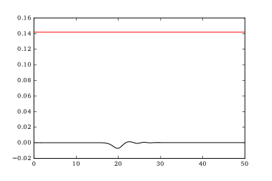
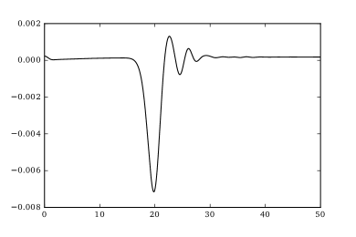
Figure 2. Left panel: Development of the Hamiltonian for total initial energy $\mathcal{H}=0.1420$, and the coupling term $\mathcal{H}_{\text{coupling}}$ for Experiment (A). Right panel: close-up of the graph of $\mathcal{H}_{\text{coupling}}$.

The first equation is a modification of the equation proposed by Whitham [28, 29]. The second one is its analogue for left-going waves. It is not known if they are well-posed even though for a large class of similar equations the answer is affirmative [13]. We shall see below that it is quite often the case that colliding waves almost do not affect each other and one may admit independence and regard basically just the equation (3.23). Up to small terms, the final result is obtained by linear superposition (3.8). Indeed in Figure 2 the dependence on time of interaction energy (3.21) for the Right-left system (3.19), (3.19) is represented. One can see that the interaction is going on for a short time and is of negligible order. This results in a small residual of solution after the interaction.

4. The numerical approach

All the models discussed in the project are solved by treating the linear part $\mathcal{L}$ and the nonlinear part $\mathcal{N}$ separately using a split-step scheme. In other words we solve a system of the form

$$z_{t}=\mathcal{L}(z)+\mathcal{N}(z)$$ (4.1)

which is treated by solving the systems $z_{t}=\mathcal{L}(z)$ and $z_{t}=\mathcal{N}(z)$. Denote by $\exp(t\mathcal{L})$ an integrator of the first one and $\exp(t\mathcal{N})$ an integrator of the the second one. We make use of a symplectic integrator of 6th order introduced by Yoshida [30]. The main advantage of such an integrator is that the time step can be made relatively large which can accelerate calculations greatly. Yoshida developed his numerical scheme for separable finite Hamiltonian systems, however, it proved to be efficient also in water wave problems [2]. Below we describe the method in application to the models derived. Following Yoshida a one step integrator for the whole system (4.1) is approximated by the product

$$\exp[\delta t(\mathcal{L}+\mathcal{N}))]=\exp(c_{1}\delta t\mathcal{L})\exp(d_{1}\delta t\mathcal{N})\exp(c_{2}\delta t\mathcal{L})\cdot\ldots\cdot\exp(d_{7}\delta t\mathcal{N})\exp(c_{8}\delta t\mathcal{L})$$

where $\delta t$ is the time step and $c_{i}$, $d_{i}$ are constants given by

$$c_{1}=c_{8}=w_{3}/2,\quad c_{2}=c_{7}=(w_{3}+w_{2})/2,\quad c_{3}=c_{6}=(w_{2}+w_{1})/2,\quad c_{4}=c_{5}=(w_{1}+w_{0})/2$$

and

$$d_{1}=d_{7}=w_{3},\quad d_{2}=d_{6}=w_{2},\quad d_{3}=d_{5}=w_{1},\quad d_{4}=w_{0}.$$

Here we take the following set of weights

$$w_{3}=0.784513610477560,\quad w_{2}=0.235573213359357,$$

$$w_{1}=-1.17767998417887,\quad w_{0}=1.315186320683906.$$

One can notice that the integrator is symmetric. The meaning of the product is that each time step is divided into substeps.

The systems $z_{t}=\mathcal{L}(z)$ and $z_{t}=\mathcal{N}(z)$ are solved using spectral methods. Moreover, the first one for each model can be solved exactly. For example, the linearization of the system (3.16)-(3.17) has the following solution

$$\eta(t)=\cos Ut\eta_{0}-iHD\frac{\sin Ut}{U}v_{0},$$

$$v(t)=-ig/H\tanh HD\frac{\sin Ut}{U}\eta_{0}+\cos Utv_{0},$$

with the initial data $\eta_{0}$, $v_{0}$. The operator $U$ has the form

$$U=\sqrt{gG_{0}}=\sqrt{gD\tanh HD}.$$ (4.2)

These formulas represent the integrator $\exp(t\mathcal{L})$ for the systems (3.16)-(3.17) and (1.5)-(1.6) since the linear part $\mathcal{L}$ is the same for those two.

For the systems (1.3)-(1.4) and (3.12)-(3.13) the integrator $\exp(t\mathcal{L})$ has the form

$$\eta(t)=\cos Ut\eta_{0}-i\tanh HD\frac{\sin Ut}{U}u_{0},$$

$$u(t)=-igD\frac{\sin Ut}{U}\eta_{0}+\cos Utu_{0},$$

with the initial data $\eta_{0}$, $u_{0}$.

For the system (3.19)-(3.20), the operator $\exp(t\mathcal{L})$ is diagonal,

$$g\mathcal{W}\partial_{x}=ig\mathcal{W}D=i\sqrt{gG_{0}}\operatorname{sgn}D,$$

and the linearized problem has the solution

$$r(t)=\exp(-itU\operatorname{sgn}D)r_{0},$$

$$s(t)=\exp(itU\operatorname{sgn}D)s_{0},$$

where $r_{0}$, $s_{0}$ are initial right- and left-going waves, respectively, and $U$ is defined by (4.2).

For all models discussed here, we use the standard Runge-Kutta scheme of 4th order as the nonlinear integrator $\exp(t\mathcal{N})$. It is explicit but not symplectic. One might argue that it makes the whole integrator $\exp(t\mathcal{L}+t\mathcal{N})$ not symplectic any more.

As an alternative we also ran all computations with a symplectic Euler scheme, such as described in [15]. This scheme turns out to be explicit for most of the models discussed here. Indeed, for example, for the ASMP model (1.3)-(1.4) one step of the semi-implicit Euler method has the form

$$\eta_{n+1} =\eta_{n}-\delta t\partial_{x}(H\mathcal{K}u_{n}+\eta_{n+1}u_{n}),$$

$$u_{n+1} =u_{n}-\delta t\partial_{x}(g\eta_{n+1}+\frac{1}{2}u_{n}^{2})$$

that can be resolved with respect to $\eta_{n+1}$ as follows. On the space $l_{2}^{N}$ define operator $B_{n}f=-\delta t\partial_{x}(u_{n}f)$ that is bounded $\lVert B_{n}\rVert\leqslant\delta tN\max u_{n}.$ Expecting uniform boundedness of solution $u$ one can choose the time step $\delta t=O(1/N)$ so that $\lVert B_{n}\rVert\leqslant C<1.$ Thus

$$(1-B_{n})\eta_{n+1}=\eta_{n}-\delta t\partial_{x}H\mathcal{K}u_{n}$$

is resolved as

$$\eta_{n+1}=(1+B_{n}+B_{n}^{2}+\ldots)(\eta_{n}-\delta t\partial_{x}H\mathcal{K}u_{n}).$$

Hence $\eta_{n+1}$, $u_{n+1}$ are resolved via $\eta_{n}$, $u_{n}$ and the scheme is explicit and symplectic at the same time.

The numerical scheme of the free-surface problem for the Euler equations is based on a time-dependent conformal mapping of the fluid domain into a strip. A complete description of the method can be found in [21, 27].

5. Numerical experiments

The model systems described above are now characterized with respect to numerical instability due to spatial discretization. For the numerical experiments we make the problem nondimensional by setting $H=1$ and $g=1$. The computational domain is $-L\leq x\leq L$, with $L=70$. Initial conditions are imposed by means of

$$\eta_{0}(x;x_{0},a,\lambda)=a\cdot\operatorname{sech}^{2}(f(x-x_{0}))-C,$$ (5.1)

where

$$f(\lambda)=\frac{2}{\lambda}\log\left(1+\sqrt{2}\right),\qquad C(\lambda)=\frac{a}{2fL}\left(\tanh f(L-x_{0})+\tanh f(L+x_{0})\right).$$

Here $C(\lambda)$ and $f(\lambda)$ are chosen so that $\int_{-L}^{L}\eta_{0}(x)dx=0$, and the wave-length $\lambda$ is the distance between the two points $x_{1}$ and $x_{2}$ at which $\eta_{0}(x_{1})=\eta_{0}(x_{2})=a/2$. Below we always take the wave-length $\lambda=\sqrt{5}$.

In all problems below we are interested in time evolution from $t_{0}=0$ to $t_{max}=50$. In cases of collision of two waves we send them towards each other. So first of all we simulate problems that cannot be described by unidirectional models like KdV or Whitham equations. Secondly, one can see that all the models introduced are in line with the effect of quasi-elastic interaction of waves. So after collision waves behave as independent with slight tails. In all experiments below we provide initial data $\eta(x,0)$ and $\Phi(x,0)$ for the Euler system. Initial data for the approximate models can easily be obtained by applying transformations of variables $u(x,0)=\partial_{x}\Phi(x,0)$, (3.4) and (3.7). According to (3.8) one can make quasi-right moving waves taking the surface velocity $u(x,0)=\mathcal{W}^{-1}\eta(x,0)$.

As was already said the splitting method we are making use of allows us to take relatively large time steps. So we take $\delta t=0.05$ when the number of Fourier harmonics is either $N=512$ or $N=1024$. This choice is dictated by the stiffness of the ASMP model (1.3)-(1.4) since the scheme becomes unstable for large $N$ and might need filtering due to the probable ill-posedness of the model. In comparative experiments, on the other hand, we do not want to use any filtration.

Experiment 5.1 (A).

Consider a collision of two approaching positive waves. Let $a=0.2$ and $x_{0}=20$. Impose initial surface

$$\eta(x,0)=\eta_{0}(x;x_{0})+\eta_{0}(x;-x_{0})$$

and initial potential

$$\Phi(x,0)=-\int_{0}^{x}\mathcal{W}^{-1}\eta_{0}(\xi;x_{0})d\xi+\int_{0}^{x}\mathcal{W}^{-1}\eta_{0}(\xi;-x_{0})d\xi.$$

All approximate systems in Experiment (A) are solved on the grid with $N=1024$.

Experiment 5.2 (B).

Consider a collision of a trough and a convex wave. Let $a=0.1$ and $x_{0}=20$. Impose initial surface

$$\eta(x,0)=\eta_{0}(x;x_{0})-\eta_{0}(x;-x_{0})$$

and initial potential

$$\Phi(x,0)=-\int_{0}^{x}\mathcal{W}^{-1}\eta_{0}(\xi;x_{0})d\xi-\int_{0}^{x}\mathcal{W}^{-1}\eta_{0}(\xi;-x_{0})d\xi.$$

All approximate systems in Experiment (B) are solved on the grid with $N=512$.

Experiment 5.3 (C).

Consider a collision of two troughs. Let $a=0.1$ and $x_{0}=20$. Impose initial surface

$$\eta(x,0)=-\eta_{0}(x;x_{0})-\eta_{0}(x;-x_{0})$$

and initial potential

$$\Phi(x,0)=\int_{0}^{x}\mathcal{W}^{-1}\eta_{0}(\xi;x_{0})d\xi-\int_{0}^{x}\mathcal{W}^{-1}\eta_{0}(\xi;-x_{0})d\xi.$$

All approximate systems in Experiment (C) are solved on the grid with $N=512$.

Experiment 5.4 (E1-E3).

Consider the evolution of waves with the initial surface elevation

$$\eta(x,0)=\eta_{0}(x;x_{0}=0)$$

where $a=0.3$ and $x_{0}=0$. Impose firstly (E1) initial potential

$$\Phi(x,0)=\int_{0}^{x}\mathcal{W}^{-1}\eta_{0}(\xi)d\xi,$$

than secondly (E2) initial potential

$$\Phi(x,0)=\int_{0}^{x}\eta_{0}(\xi)d\xi,$$

and finely (E3) initial potential

$$\Phi(x,0)=0.$$

All approximate systems in Experiments (E1-E3) are solved on the grid with $N=1024$. Note that the initial potential of Experiment (E2) creates only approximately a right-going wave according to the linear long wave theory. Anyway neither the conditions of Experiment (E1) or of Experiment (E2) induce completely one way propagation as numerical results shows. Surprisingly, initial potentials of the type as in Experiment (E3) lead to better correspondence between approximate models and the Euler system then initial potentials of the type as in Experiment (E2). And moreover, of the type as in Experiment (E2) lead to the better correspondence then of the type as in Experiment (E1). We believe it is mainly a technical feature since the initial error of evaluation surface potential via $\mathcal{W}^{-1}$ and integration normally increases with the time.

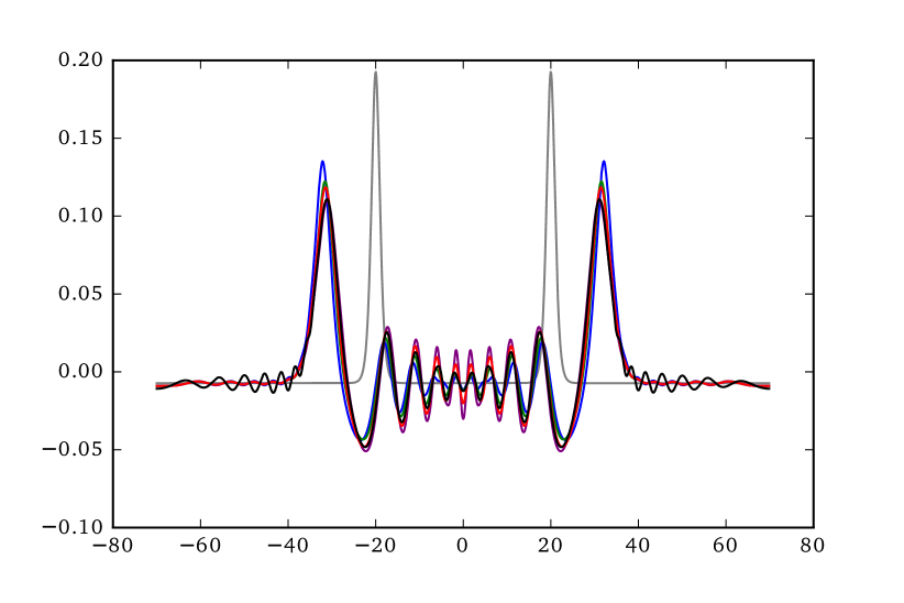
Figure 1. Experiment (A). The thin grey curve represents the initial data. The black curve is the approximate solution of the full Euler system at $t=50$. The color coding is as follows: purple – Hamiltonian HP system; red – right-left system; blue – ASMP system; green – HP system.

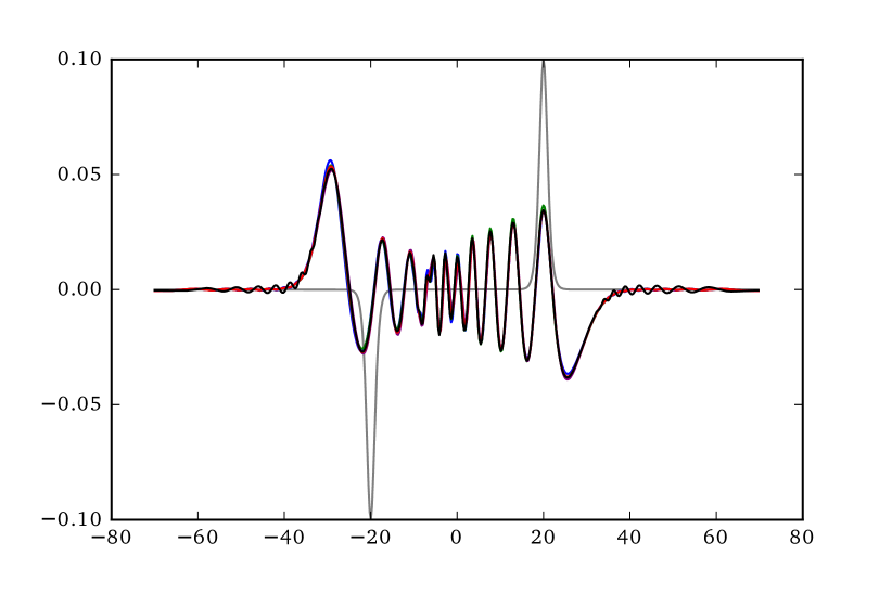
Figure 3. Experiment (B). The thin grey curve represents the initial data. The black curve is the approximate solution of the full Euler system at $t=50$. The color coding is as follows: purple – Hamiltonian HP system; red – right-left system; blue – ASMP system; green – HP system.

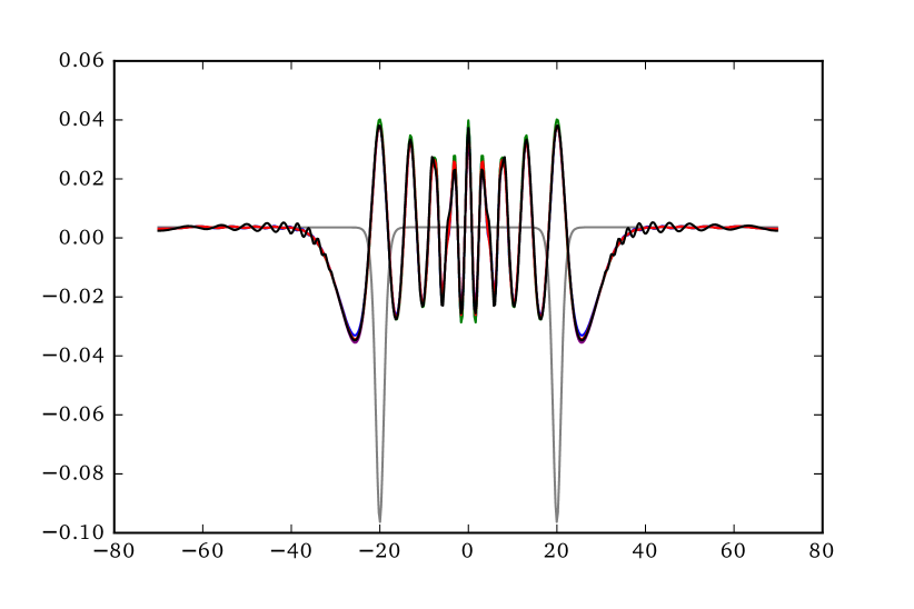
Figure 4. Experiment (C). The thin grey curve represents the initial data. The black curve is the approximate solution of the full Euler system at $t=50$. The color coding is as follows: purple – Hamiltonian HP system; red – right-left system; blue – ASMP system; green – HP system.

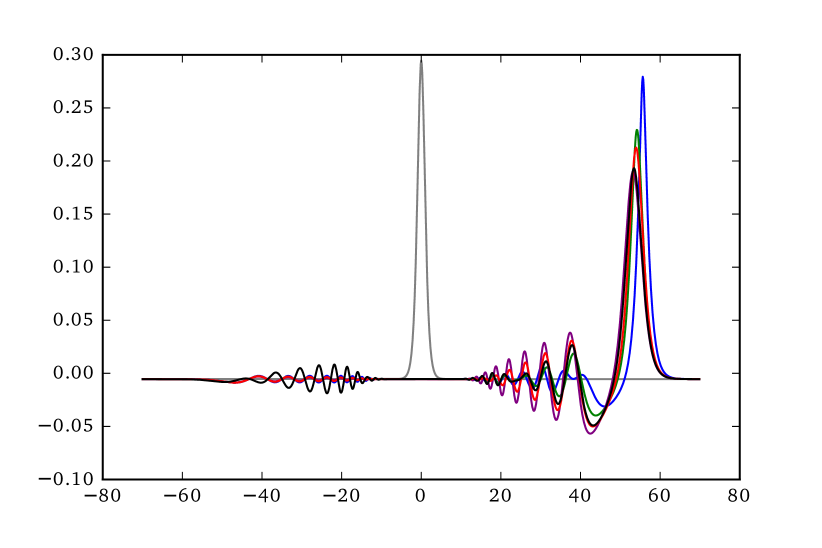
Figure 5. Experiment (E1). The thin grey curve represents the initial data. The black curve is the approximate solution of the full Euler system at $t=50$. The color coding is as follows: purple – Hamiltonian HP system; red – right-left system; blue – ASMP system; green – HP system.

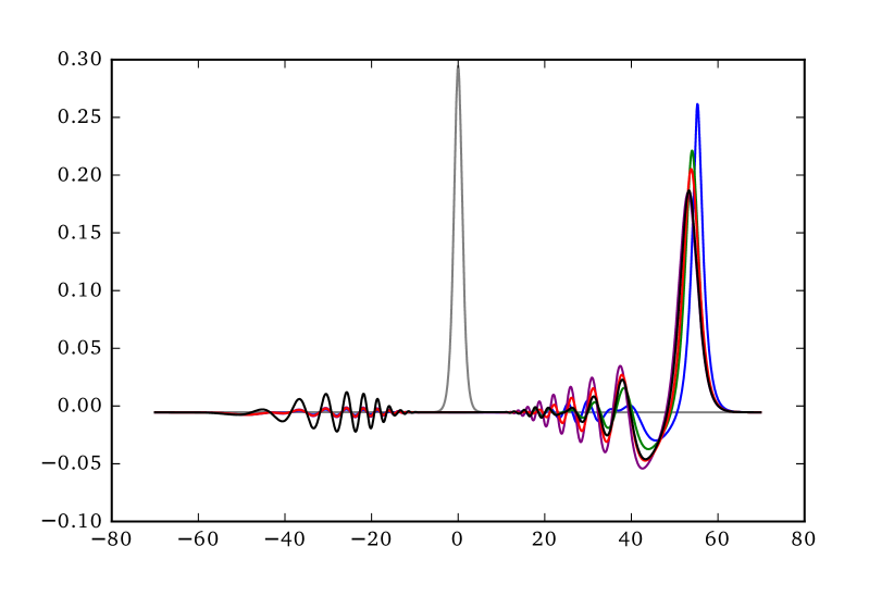
Figure 6. Experiment (E2). The thin grey curve represents the initial data. The black curve is the approximate solution of the full Euler system at $t=50$. The color coding is as follows: purple – Hamiltonian HP system; red – right-left system; blue – ASMP system; green – HP system.

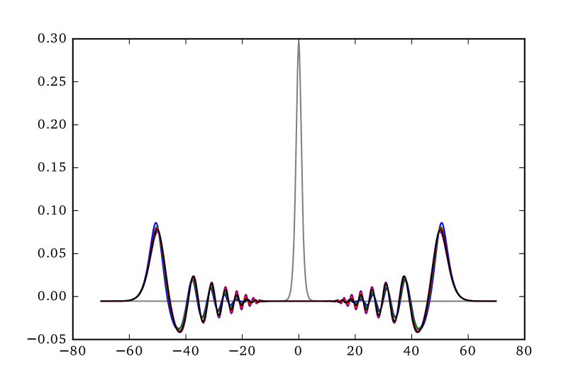
Figure 7. Experiment (E3). The thin grey curve represents the initial data. The black curve is the approximate solution of the full Euler system at $t=50$. The color coding is as follows: purple – Hamiltonian HP system; red – right-left system; blue – ASMP system; green – HP system.

In all presented figures initial elevation profiles are marked by grey lines. Solutions of the Euler system (2.1)-(2.4) are black, of the ASMP system (1.3)-(1.4) are blue, of the Hur–Pandey system (1.5)-(1.6) are green, of the Hamiltonian Hur–Pandey system (3.16)-(3.17) are purple, and of the right-left system (3.19)-(3.20) are red.

Experiment	A	B	C	E1	E2	E3
Euler	0.1316	0.0329075955585	0.03291	0.1481	0.1398	0.0740610317118
ASMP	0.1440	0.0329075170851	0.03136	0.1686	0.1569	0.0740419134333
Hamiltonian HP	0.1405	0.0329075170854	0.03180	0.1626	0.1524	0.0740419134422
Right–Left	0.1420	0.0329075170854	0.03162	0.1651	0.1543	0.0740419134422

Table 1. Hamiltonians $\mathcal{H}$ for various systems, evaluated at $t=50$.

Experiment	A	B	C	E1	E2	E3
ASMP	0.488	0.109	0.149	0.883	0.768	0.153
Hur–Pandey	0.253	0.085	0.126	0.339	0.315	0.082
Hamiltonian HP	0.167	0.130	0.106	0.231	0.207	0.061
Right–Left	0.167	0.089	0.128	0.240	0.218	0.048

Table 2. Errors $\mathcal{E}$, evaluated at $t=50$.

In order to quantitatively compare the accuracy of each approximate model we calculate the differences between Euler solutions and solutions of each system correspondingly. These errors are measured in the integral $L^{2}$-norm normalized by initial condition as follows

$$\mathcal{E}=\frac{\lVert\eta_{Euler}-\eta_{model}\rVert}{\lVert\eta_{initial}\rVert}$$

where

$$\lVert\eta_{Euler}-\eta_{model}\rVert=\max_{t}\sqrt{\int(\eta_{Euler}(x,t)-\eta_{model}(x,t))^{2}dx}$$

and

$$\lVert\eta_{initial}\rVert=\sqrt{\int\eta(x,0)^{2}dx}.$$

Here $\eta_{Euler}(x,t)$ is the solution for the Euler system and $\eta_{model}(x,t)$ corresponds either to ASMP, Hur–Pandey, Hamiltonian Hur–Pandey or Right–Left system. The corresponding results are represented in Table 2.

As was stated above some models work better in the sense of numerical stability. There were many discussions about ill-posedness of ASMP model [3]. In the next experiment we provide an example with initial data satisfying the condition for local well posedness. One can see that the initial data is lifted over the real axis so the mean value is approximately 0.35. It is known from Ehrnström, Pei, Wang [14] that we are in a locally well posed situation, however, the obtained solution seems very unstable as one can see in Figure 8. This experiment was repeated with different time integrators, including the symplectic first-order Euler method described in Section 4. The results were always the same, pointing to doubts about the long-time well posedness of the ASMP system.

In order to systematize our experiments regarding the well posedness and stability of the Whitham systems, we used the following initial data:

Experiment 5.5.

Suppose we have a trough with amplitude $a=0.3$. Let $x_{0}=0$. Solve System (1.3)-(1.4) with the initial surface

$$\eta(x,0)=-\eta_{0}(x)+0.35$$

and the initial velocity

$$u(x,0)=\mathcal{W}^{-1}\eta(x,0).$$

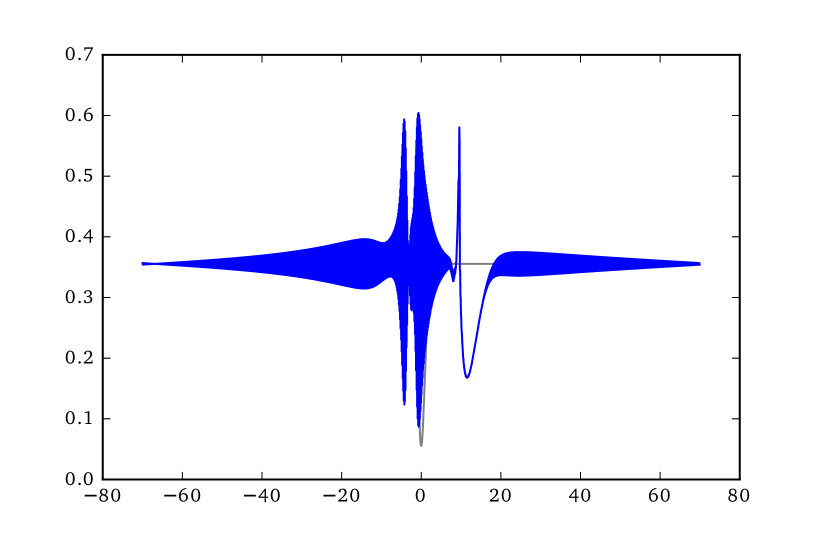
Figure 8. Approximate solution of the ASMP Whitham system with initial data satisfying the condition $\inf{\eta_{0}}>0$.

Problems with the HP system (1.5)-(1.6) may occur if an initial trough is deep enough. In the example shown on Figure 9 we have to filter half of the high Fourier modes to make computations stable. The resulting noisy solution continues its propagation and one can notice that all the oscillations happen around some reasonable mean curve that can be obtained easily by solving either the system (3.16)-(3.17) or the system (3.19)-(3.20) without any filtration. The results are represented on Figure 9.

Experiment 5.6.

Suppose $a=0.6$ and $x_{0}=0$. Solve System (1.5)-(1.6) with initial surface

$$\eta(x,0)=-\eta_{0}(x)$$

and initial velocity

$$v(x,0)=\mathcal{K}\mathcal{W}^{-1}\eta(x,0).$$

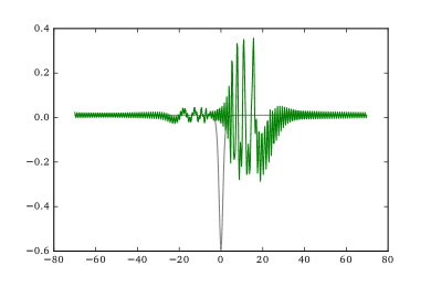
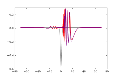
Figure 9. Left panel: De-aliased solution of the HP system with N = 512 and time step = 0.05. Snapshot is taken at $t=25$. Right panel: The same for Hamiltonian version of the HP system and the Right–Left system.

As to numerical stability of the Right–Left system (3.19)-(3.20), we can notice that this system encountered problems only in extreme non-physical situations, as for example, with an initial deep trough of amplitude $a=1.2$ and increasing number of harmonics up to $N=2^{15}$. The Hamiltonian version of the Hur–Pandey system (3.16)–(3.17) is numerically stable even in such a physically absurd problem.

Finally, let us look at the development of the Hamiltonian in two cases. First, an example of self-stabilization in the Matsuno system:

Experiment 5.7.

Suppose $a=0.2$ and $x_{0}=0$. Solve Matsuno System (3.12)-(3.13) with initial surface $\eta(x,0)=\eta_{0}(x)$ and initial velocity $u(x,0)=\mathcal{K}\mathcal{W}^{-1}\eta(x,0).$ We take the time step $\delta t=0.1$ and the number of grid points $N=512$.

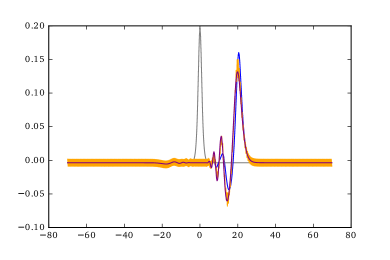
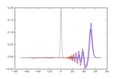
Figure 10. Self-stabilized solution of Matsuno system with $N=512$ and time step $\delta t=0.1$. Left panel: $t=20$, right panel: $t=50$.

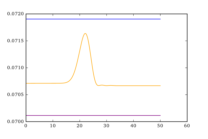
Figure 11. Total energy of the self-stabilized solution of Matsuno system as a function of time $t$, with $N=512$ and time step $\delta t=0.1$.

One might think that a numerical method conserving the total energy could remove the instabilities in the solution. Unfortunately this is not the case. We applied a simple projection method [15] to obtain a conservative method. With this method, energy was indeed conserved, and we managed to get a constant instead of the time-varying energy shown in Figure 11. However, the solutions itself remained noisy such as in Figure 10, and the computational cost is substantially higher than in the nonconservative method.

6. Acknowledgments

This research was supported in part by the Research Council of Norway through grants 213474/F20 and 239033/F20.

References

- [1] Aceves-Sánchez, P., Minzoni, A.A. and Panayotaros, P. Numerical study of a nonlocal model for water-waves with variable depth, Wave Motion 50 (2013), 80–93.
- [2] Carter, J.D. Bidirectional Whitham equations as models of waves on shallow water, arXiv:1705.06503 (2017).
- [3] Claassen, K.M. and Johnson, M.A. Numerical bifurcation and spectral stability of wavetrains in bidirectional Whitham models, arXiv:1710.09950 (2017).
- [4] Choi, W. Nonlinear evolution equations for two-dimensional surface waves in a fluid of finite depth, J. Fluid Mech. 295 (1995), 381–394.
- [5] Craig, W. and Sulem, C. Numerical simulation of gravity waves. J. Comp. Phys. 108 (1993), 73–83.
- [6] Craig, W. and Groves, M.D. Hamiltonian long-wave approximations to the water-wave problem. Wave Motion 19 (1994), 367–389.
- [7] Craig, W., Guyenne, P. and Kalisch, H. Hamiltonian long-wave expansions for free surfaces and interfaces. Comm. Pure Appl. Math. 58 (2005), 1587–1641.
- [8] Dinvay, E., Moldabayev, D., Dutykh, D., Kalisch, H. The Whitham equation with surface tension. Nonlinear Dyn (2017). doi:10.1007/s11071-016-3299-7
- [9] M. Ehrnström, M.A. Johnson and K.M. Claassen, Existence of a highest wave in a fully dispersive two-way shallow water model, arXiv preprint arXiv:1610.02603
- [10] Dinvay, E., Kalisch, H., Moldabayev, D., Parau, E., The Whitham equation for hydroelastic waves, submitted.
- [11] Ehrnström, M., Kalisch, H. Traveling waves for the Whitham equation. Diff. Int. Eq. 22 (2009), 1193–1210
- [12] Ehrnström, M., Kalisch, H. Global bifurcation for the Whitham equation. Math. Modelling Natural Phenomena 8 (2013), 13–30.
- [13] M. Ehrnström, L. Pei. Classical well-posedness in dispersive equations with nonlinearities of mild regularity, and a composition theorem in Besov spaces, arXiv e-prints, September 2017.
- [14] M. Ehrnström, L. Pei, and Y. Wang. A conditional well-posedness result for the bidirectional Whitham equation, arXiv e-prints, August 2017.
- [15] Ernst Hairer, Gerhard Wanner, Christian Lubich. Geometric Numerical Integration. Structure-Preserving Algorithms for Ordinary Differential Equations (Springer, 2006).
- [16] Hur, V.M. and Johnson, M. Modulational instability in the Whitham equation of water waves. Studies in Applied Mathematics 134 (2015), 120–143.
- [17] Hur, V.M. and Pandey, A.K. Modulational instability in a full-dispersion shallow water model. arXiv:1608.04685 (2016).
- [18] Lannes, D. The Water Waves Problem. Mathematical Surveys and Monographs, vol. 188 (Amer. Math. Soc., Providence, 2013).
- [19] Lannes, D. and Bonneton, P. Derivation of asymptotic two-dimensional time-dependent equations for surface water wave propagation Phys. Fluids 21 (2009), 016601.
- [20] Lannes, D. and Saut, J.-C. Remarks on the full dispersion Kadomtsev-Petviashvili equation. Kinet. Relat. Models 6 (2013), 989–1009.
- [21] Li, Y. A., Hyman, J. M. and Choi, W. A Numerical Study of the Exact Evolution Equations for Surface Waves in Water of Finite Depth. Stud. Appl. Math. 113 (2004), 303–324.
- [22] Linares, F., Pilod, D. and Saut, J.-C. Dispersive perturbations of Burgers and hyperbolic equations I: local theory. SIAM J. Math. Anal. 46 (2014), 1505–1537.
- [23] Matsuno, Y. Two-dimensional evolution of surface gravity waves on a fluid of arbitrary depth, Phys. Rev. E 47 (1993), 5493-5496.
- [24] Moldabayev, D., Kalisch, H. and Dutykh, D. The Whitham Equation as a model for surface water waves, Phys. D 309 (2015), 99–107.
- [25] Sanford, N., Kodama, K., Carter, J.D. and Kalisch, H. Stability of traveling wave solutions to the Whitham equation. Phys. Lett. A 378 (2014), 2100–2107.
- [26] Vargas-Magana, R.M. and Panayotaros, P. A Whitham-Boussinesq long-wave model for variable topography, Wave Motion 65 (2016), 156–174.
- [27] Viotti, C., Dutykh, D., & Dias, F. (2013). The conformal-mapping method for surface gravity waves in the presence of variable bathymetry and mean current. In Procedia IUTAM (Vol. 11, pp. 110–118). https://doi.org/10.1016/j.piutam.2014.01.053
- [28] Whitham, G. B. Variational methods and applications to water waves. Proc. Roy. Soc. London A 299 (1967), 6–25.
- [29] Whitham, G. B. Linear and Nonlinear Waves (Wiley, New York, 1974).
- [30] H. Yoshida, Construction of higher order symplectic integrators, Physics Letters A 150 (1990) 262–268.
- [31] Zakharov, V.E. Stability of periodic waves of finite amplitude on the surface of a deep fluid. J. Appl. Mech. Tech. Phys. 9 (1968), 190–194.