A multifiltering study of turbulence in a large sample of simulated galaxy clusters

Abstract

We present results from a large set of N-body/SPH hydrodynamical cluster simulations aimed at studying the statistical properties of turbulence in the ICM. The numerical hydrodynamical scheme employs a SPH formulation in which gradient errors are strongly reduced by using an integral approach. We consider both adiabatic and radiative simulations. We construct clusters subsamples according to the cluster dynamical status or gas physical modeling, from which we extract small-scale turbulent velocities obtained by applying to cluster velocities different multiscale filtering methods. The velocity power spectra of non-radiative relaxed clusters are mostly solenoidal and exhibit a peak at wavenumbers set by the injection scales $\simeq r_{200}/10$, at higher wavenumbers the spectra are steeper than Kolgomorov. Cooling runs are distinguished by much shallower spectra, a feature which we interpret as the injection of turbulence at small scales due to the interaction of compact cool gas cores with the ICM. Turbulence in galaxy clusters is then characterized by multiple injection scales, with the small scale driving source acting in addition to the large scale injection mechanisms. Cooling runs of relaxed clusters exhibit enstrophy profiles with a power-law behavior over more than two decades in radius, and a turbulent-to-thermal energy ratio $\lower 2.15277pt\hbox{$\;\buildrel<\over{\sim}\;$}1\%$. In accord with Hitomi observations, in the core of a highly relaxed cluster we find low level of gas motions. In addition, the estimated cluster radial profile of the sloshing oscillation period is in very good agreement with recent Fornax measurements, with the associated Froude number satisfying $Fr\lower 2.15277pt\hbox{$\;\buildrel<\over{\sim}\;$}0.1$ within $r/r_{200}\lower 2.15277pt\hbox{$\;\buildrel<\over{\sim}\;$}0.1$. Our findings suggest that in cluster cores ICM turbulence approaches a stratified anisotropic regime, with weak stirring motions dominated by gravity buoyancy forces and strongly suppressed along the radial direction. We conclude that turbulent heating cannot be considered the main heating source in cluster cores.

1 Introduction

In the standard hierarchical scenario galaxy clusters are the most recent and massive virialized objects formed in the Universe. Gas falling into the dark matter potential during the formation processes will be heated to virial temperatures ($\sim 10^{7}-10^{8}\kern 2.0pt{}^{\circ}{\kern-2.0ptK}$) and at equilibrium will reside in the form of a fully ionized X-ray emitting intracluster medium (ICM). During the process of cluster formation, large scale motions driven by merging and accretion processes will generate hydrodynamic instabilities which will inject turbulence into the ICM. Large eddies at the injection scale will form smaller eddies which will transfer energy down to the dissipative scale, thus heating the ICM. This scenario is supported both observationally and numerically (Brüggen & Vazza, 2015, and references cited therein).

Turbulence in the ICM can be detected either directly using high resolution X-ray spectroscopy to measure emission-line broadening and thus turbulent velocities, or indirectly through a number of effects influencing the physics of the ICM. Indirect evidence for the presence of turbulence in the ICM has been obtained by measuring the fluctuation spectra of X-ray surface brightness maps (Schuecker et al., 2004; Gaspari & Churazov, 2013), resonant scattering effects (Churazov et al., 2004; Ogorzalek et al., 2017), Sunyaev-Zeldovich (SZ) fluctuations (Battaglia at al., 2012), and through the diffusion of metals in the ICM (Rebusco et al., 2006). The first direct detection of turbulence in the ICM has been provided recently by the Hitomi collaboration et al. (2016, hereafter H16), who measured turbulent velocities of the order of $150~{}kms^{-1}$ in the core of the Perseus cluster.

Observational support for the presence of turbulence in the ICM favors a low-viscosity or inviscid ICM. This is confirmed by the presence (Ichinohe et al., 2017; Su et al., 2017a) of Kelvin-Helmholtz instabilities (KHI) at sloshing cold fronts (Markevitch & Vikhlinin, 2007). These KHI would otherwise be suppressed in a viscous ICM (ZuHone et al., 2011; Roediger et al., 2013). However, these conclusions may be too simplistic. Constraints on ICM viscosity may be affected by projection effects in the case of Perseus (ZuHone et al., 2018), or by the presence of magnetic fields which impact on the small-scale transport properties of the plasma (Schmidt et al., 2017; Bambic et al., 2018; Barnes et al., 2018).

However, additional support for a low-viscosity ICM comes from measurements of ICM density fluctuation amplitudes (Gaspari & Churazov, 2013; Eckert et al., 2017), which indicate an ICM with strongly suppressed conduction with respect to the Spitzer value.

Turbulent motions are expected to affect ICM properties in a variety of ways. For instance, the accuracy of cosmological constraints extracted from galaxy clusters relies on accurate measurements of their gravitating mass. X-ray estimates of cluster masses are based on the assumption of spherical symmetry and hydrostatic equilibrium (Rasia et al., 2006; Nagai et al., 2007a; Piffaretti & Valdarnini, 2008; Lau et al., 2009; Biffi et al., 2016). However, turbulent motions will provide additional non-thermal pressure support which will bias the hydrostatic equilibrium assumption.

Additionally, non-thermal pressure support also has a significant effect on the shape and amplitude of the thermal SZ power spectrum (Shaw et al, 2010), The SZ effect is due to inverse Compton scattering from CMB photons. Because of its linear dependency on gas density, it can be used to derive independent cosmological constraints from SZ cluster surveys (Shaw et al, 2010; Battaglia at al., 2012).

Other physical processes in the ICM for which the role of turbulence is important are the amplification of magnetic fields (Dolag et al., 2002; Beresnyak & Miniati, 2016; Vazza et al, 2018), cosmic ray re-acceleration (Eckert et al., 2017), and transport of metals (Rebusco et al., 2006).

Finally, turbulence in the ICM has been also proposed as a possible heating source to solve the so-called cooling flow problem. The center of relaxed clusters is often characterized by the presence of cool dense cores with cooling times $\lower 2.15277pt\hbox{$\;\buildrel<\over{\sim}\;$}1Gyr$, shorter than the age of the Universe. This implies radiative losses which will lead to an inward motion producing a ‘cooling flow’ (Fabian, 1994) and large mass accretion rates. This is not observed (Peterson et al., 2003; Sanders et al., 2008), and some heating sources must be operating in the cluster cores to regulate the cooling flows.

Various heating models have been proposed in the literature to balance radiative cooling in cluster cores and to solve the cooling flow problem. Possible physical mechanisms include thermal conduction (Yang & Reynolds, 2016a), dynamical friction due to galaxy motions (El-Zant et al., 2004; Kim, 2007) or turbulent diffusion (Ruszkowski & Oh, 2011), turbulent heating (Fujita et al., 2004; Dennis & Chandran, 2005; Zhuravleva et al., 2014a), sound wave dissipation (Zweibel et al., 2018), and feedback from active galactic nuclei (AGN).

In the latter scenario, the ICM is heated by interaction with buoyantly rising bubbles due to the injection of jets launched from the central AGN. This heating model appears to be very promising, since it is energetically viable and is supported by X-ray observations of bubbles or cavities (Fabian, 2012). However, the physical processes for which the jet mechanical energy is transferred to the ICM thermal energy are not yet well understood and considerable effort has gone into investigating (Socker, 2016, and references cited therein) how the ICM is thermalized in the proposed scenario.

Numerical simulations are a necessary tool for investigating self-consistently the hydrodynamical flows that take place during merging and accretion processes driving the ICM evolution and, in turn, the generation of turbulence. The role of turbulence in hydrodynamical simulations of galaxy clusters has been investigated by many authors (Fujita et al., 2004; Dolag et al., 2005; Iapichino & Niemeyer, 2008; Maier et al., 2009; Vazza et al., 2009a; Valdarnini, 2011; Iapichino et al., 2011; Vazza et al., 2012; Miniati, 2014, 2015; Schmidt et al., 2016; Iapichino et al., 2017; Schmidt et al., 2017; Vazza et al., 2017; Wittor et al., 2017).

A critical issue when analyzing simulation results is the separation of small-scale chaotic turbulent motion from large scale coherent bulk flows. In this context several strategies have been proposed based on the use of low-pass filters (Dolag et al., 2005; Valdarnini, 2011; Vazza et al., 2012, 2017), subgrid modeling (Maier et al., 2009), adaptive Kalman filtering (Schmidt et al., 2016), and wavelets (Shi et al., 2018). In particular, Vazza et al. (2012) developed an iterative multi-scale filtering approach to extract turbulent motions from cluster velocities. We will later discuss their method in detail, since it will be applied, with some modifications, to the simulations presented here.

All of the simulation papers previously cited have used codes based on Eulerian schemes (Stone & Norman, 1992; Stone et al., 2008; Fryxell et al., 2000; Teyssier, 2002; Norman, 2005; Bryan et al., 2014), with the exceptions of Dolag et al. (2005) and Valdarnini (2011) who employed a Lagrangian smoothed particle hydrodynamics (SPH) code (Gingold & Monaghan, 1977; Lucy, 1977; Hernquist & Katz, 1989)

The SPH code has several advantages, which are very useful in astrophysics problems. Because of its Lagrangian nature, SPH can naturally follow the development of large matter concentrations. Moreover, the method is Galilean invariant and naturally conserves linear and angular momentum.

However, it is well known that in its standard formulation SPH suffers from several difficulties (see, for example, Valdarnini, 2016, and references cited therein). A first problem of standard SPH is the difficulty in dealing with steep density gradients present at the interface of contact discontinuities; this is the so-called local mixing instability (LMI: Price, 2008; Read et al., 2010).

Several variants have been proposed for solving this problem; here we follow the approach of Price (2008), who incorporated an artificial conductivity term into the SPH thermal equation. This term is aimed at smoothing thermal energy at the borders of contact discontinuities, which is equivalent to adding a heat diffusion term to the SPH equations. By introducing this term, it is found (Wadsley et al., 2008; Valdarnini, 2012) that in non-radiative simulations of galaxy clusters, the levels of core entropies are then in agreement with those produced using grid codes.

The second problem is related to sampling effects. Because a finite number of particles is used to model the fluid, the discretization implies the presence of zeroth-order errors in the momentum equation (Read et al., 2010). To overcome this problem, among other approaches, García-Senz et al. (2012) proposed estimating SPH gradients by evaluating integrals and performing a matrix inversion. This tensor approach has been tested in in a variety of hydrodynamical test cases (García-Senz et al., 2012; Rosswog, 2015; Valdarnini, 2016; Cabezón, et al., 2017), with good results.

In particular, it has been found that the scheme greatly improves the numerical modeling of subsonic turbulence (Valdarnini, 2016). This is a crucial issue, since it implies that the new SPH formulation can be profitably used in simulations of galaxy clusters aimed at studying turbulence.

We have incorporated this scheme into our SPH code, which has been used to construct large samples of simulated galaxy clusters. The cluster simulations were constructed according to the zoom-in method in which initial conditions for the individual SPH hydrodynamical runs were extracted from cosmological dark matter simulations of different box sizes. Our final samples comprise $\simeq 200$ clusters, with a virial mass range spanning about two orders in magnitude, from $\simeq 10^{13}\rm{\,M_{\odot}}$ up to $\simeq 10^{15}\rm{\,M_{\odot}}$.

For each cluster we ran an adiabatic gas dynamical simulation as well as a radiative run in which the physical modeling of the gas includes radiative cooling, star formation, and energy feedback from supernovae. Finally, we have used the cluster dynamical status to construct two cluster subsamples, which are identified by including the most relaxed and unrelaxed sample clusters.

The simulation suites are then used to study the statistical properties of ICM turbulence by applying a variety of multifiltering algorithms to the gas velocities of the simulation samples. The comparison between different results is also aimed at identifying the optimal filtering strategy, when in the presence of clusters with very different dynamical histories. Additionally, we also studied the turbulent profiles of an individual highly relaxed cluster which we identify as a cool-core cluster.

The paper is structured as follows. In Sect. 2 we present the numerical method. The construction of the set of simulated clusters is described in Sect. 3. In Sect. 4 we describe the methods we use to quantify the statistical properties of turbulence, together with the multifiltering strategies used to identify turbulent motions. The results are presented in Sect. 5 and our conclusions are summarized in Sect. 6.

2 Code description

This section describes the main features of the adopted hydrodynamical numerical scheme, for a general review of the SPH method see Price (2012a).

2.1 Basic equations

In SPH, the hydrodynamic fluid equations are derived from a set of point particles with mass $m_{i}$, velocity $\vec{v}_{i}$, density $\rho_{i}$, and specific entropy $A_{i}$ . We integrate here the entropy per particle, this is connected to the thermal energy per unit mass $u_{i}$ via the the particle pressure : $P_{i}=A_{i}\rho_{i}^{\gamma}=(\gamma-1)\rho_{i}u_{i}$, where $\gamma=5/3$ for a mono-atomic gas. The SPH density estimator evaluates the density at the particle position $\vec{r}_{i}$ by summing over neighboring particles $j$

$$\rho_{i}=\sum_{j}m_{j}W(|\vec{r}_{ij}|,h_{i}),$$ (1)

where $W(|\vec{r}_{i}-\vec{r}_{j}|,h_{i})$ is a kernel with compact support which is zero for $|\vec{r}_{i}-\vec{r}_{j}|\geq\zeta h_{i}$ (Price, 2012a). Throughout this paper, we will present simulation results obtained using the cubic B-spline $M_{4}$ kernel, for which $\zeta=2$.

The smoothing length $h_{i}$ is determined by the implicit equation

$$h_{i}=\eta(m_{i}/\rho_{i})^{1/3}~{},$$ (2)

so that $N_{nn}={4\pi(2\eta)^{3}}/{3}$ is the number of neighbors within a radius $2h_{i}$. Here we solve numerically the equation for the $h_{i}$ with $N_{nn}=32$.

The Euler equations can then be derived from a Lagrangian (Price, 2012a); and the momentum equation is

$$\frac{d\vec{v}_{i}}{dt}=-\sum_{j}m_{j}\left[\frac{P_{i}}{\Omega_{i}\rho_{i}^{2}}\vec{\nabla}_{i}W_{ij}(h_{i})+\frac{P_{j}}{\Omega_{j}\rho_{j}^{2}}\vec{\nabla}_{i}W_{ij}(h_{j})\right]~{},$$ (3)

where $\Omega_{i}$ is defined as

$$\Omega_{i}=\left[1-\frac{\partial h_{i}}{\partial\rho_{i}}\sum_{k}m_{k}\frac{\partial W_{ik}(h_{i})}{\partial h_{i}}\right]~{}.$$ (4)

In the next section we will present the integral method and show how this equation needs to be modified.

2.2 The Integral method

A long standing problem of classic SPH has been the presence of zeroth-order errors in gradient estimates due to sampling effects (Read et al., 2010). These errors impact on the momentum equation and degrade code performances in subsonic flows (Valdarnini, 2016). This has led many authors to propose variants of standard SPH, see, e.g., Hopkins (2015) for an introduction to several of them.

Here we will follow the approach originally proposed by García-Senz et al. (2012), in which SPH first-order derivatives are estimated through the use of integrals. It has been shown that this approach greatly improves gradient estimates (García-Senz et al., 2012; Rosswog, 2015; Valdarnini, 2016; Cabezón, et al., 2017), thus strongly reducing the noise present in the standard formulation. We briefly outline here the essential features of the method.

The gradient of a continuous function $f(\vec{r})$ can be evaluated by first defining the integral

$${I(\vec{r})}=\int_{V}\left[f(\vec{r}^{\prime})-f(\vec{r})\right]\vec{\Delta}W(|\vec{r}^{\prime}-\vec{r}|,h)d^{3}r^{\prime}~{},$$ (5)

where $\vec{\Delta}\equiv(\vec{r}^{\prime}-\vec{r})$ and $W$ is a generic spherically symmetric kernel. A Taylor expansion of $f(\vec{r}^{\prime})$ to first order can be inverted to give

$$\vec{\nabla}_{\alpha}f=\left[\tau\right]^{-1}_{\alpha\beta}I_{\beta}~{},$$ (6)

where

$$\tau_{\alpha\beta}=\tau_{\beta\alpha}=\int\Delta_{\alpha}\Delta_{\beta}Wd^{3}r^{\prime}~{}$$ (7)

are the elements of the matrix $\mathcal{T}=\{\tau\}_{\alpha\beta}$.

We must now translate the continuous version of these equations into their SPH discrete counterparts. The integral (5) becomes

$${I}_{\beta}(i)=\sum_{j}\frac{m_{j}}{\rho_{j}}f_{j}\Delta_{\beta}^{ji}W(r_{ij},h_{i})~{},$$ (8)

and for the matrix $\mathcal{T}$ of particle $i$ one has

$$\tau_{\alpha\beta}(i)=\sum_{j}\frac{m_{j}}{\rho_{j}}\Delta_{\alpha}^{ji}\Delta_{\beta}^{ji}W(r_{ij},h_{i})~{}.$$ (9)

A key step is the use of expression (8) to evaluate the integral (5), this is a valid approximation as long as the condition

$$\sum_{j}\frac{m_{j}}{\rho_{j}}(\vec{r}_{j}-\vec{r}_{i})W_{ij}\simeq 0$$ (10)

is satisfied with a certain degree of accuracy. This is crucial because it is easily shown (García-Senz et al., 2012) that the gradient approximation (6) is now antisymmetric in the exchange of the pairs $ij$, so that the new scheme maintains exact conservation properties.

The validity of the approximations involving the integral methods has been tested in a variety of hydrodynamical problems (García-Senz et al., 2012; Rosswog, 2015; Valdarnini, 2016), showing a strong decrease of errors in gradient estimates and leading to a significant improvement in code performance.

To summarize, the adoption of the integral scheme requires the evaluation of the $3\times 3$ matrix (9 ) and its inversion. This is in order to substitute in the SPH equations the scalars $\left[\vec{\nabla}_{i}W_{ik}\right]_{\alpha}$ with the following prescriptions:

$$\left[\nabla_{i}W_{ik}(h_{i})\right]_{\alpha}\rightarrow\sum_{\beta}C_{\alpha\beta}(i)\Delta_{\beta}^{ki}W(r_{ik},h_{i})\equiv{\mathcal{A}}_{\alpha,ik}(h_{i})~{},$$ (11)

and

$$\left[\nabla_{i}W_{ik}(h_{k})\right]_{\alpha}\rightarrow\sum_{\beta}C_{\alpha\beta}(k)\Delta_{\beta}^{ki}W(r_{ik},h_{k})\equiv{\mathcal{\tilde{A}}}_{\alpha,ik}(h_{k}).$$ (12)

where $\mathcal{C}=\mathcal{T}^{-1}$. The momentum equation (3 ) then becomes

$$\frac{d\vec{v}_{i,\alpha}}{dt}=-\sum_{j}m_{j}\left[\frac{P_{i}}{\Omega_{i}\rho_{i}^{2}}{\mathcal{A}}_{\alpha,ij}(h_{i})+\frac{P_{j}}{\Omega_{j}\rho_{j}^{2}}{\mathcal{\tilde{A}}}_{\alpha,ij}(h_{j})\right]~{}.$$ (13)

From now on, we will refer to the new SPH formulation as integral SPH (ISPH). Results from simulations obtained using the classical gradient formulation will be referred to as standard SPH. Throughout this paper the velocity divergence and curl of particles will be consistently evaluated using their SPH estimators, but with the gradients now computed according to the new scheme:

$$(\vec{\nabla}\cdot\vec{v})_{i}\equiv\theta_{i}=\frac{1}{\rho_{i}}\sum_{j}\sum_{\alpha}m_{j}\left[(\vec{v}_{j}-\vec{v}_{i})_{\alpha}{\mathcal{A}}_{\alpha,ij}(h_{i})\right]~{},$$ (14)

and

$$(\vec{\nabla}\times\vec{v})_{i,\alpha}=\frac{1}{\rho_{i}}\sum_{j}\sum_{\beta,\gamma}m_{j}\left[\varepsilon_{\alpha\beta\gamma}(\vec{v}_{i}-\vec{v}_{j})_{\beta}{\mathcal{A}}_{\gamma,ij}(h_{i})\right]~{},$$ (15)

where $\varepsilon_{\alpha\beta\gamma}$ is the Levi-Civita tensor.

Finally, note that it is now common practice (Beck et al., 2016a, and references cited therein) to use Wendland kernels (Dehnen & Aly, 2012) in SPH simulations with a large number of neighbors, say $N_{nn}\lower 2.15277pt\hbox{$\;\buildrel>\over{\sim}\;$}300$.

This choice of this kernel function is motivated by the need to avoid pairing instability, which is absent in the case of the Wendland functions, when using a large neighbor number. The latter regime is necessary in order to suppress errors in gradient estimates, which, as previously outlined, is a shortcoming of standard SPH.

However, in a battery of hydrodynamical tests (Valdarnini, 2016) it has been found that ISPH by far outperforms standard SPH. The zeroth-order errors in the momentum equations being reduced by many orders of magnitude, with the accuracy of the results in the regime of subsonic flows which is found comparable to that of mesh-based codes. These results then demonstrate that with the new method it is not necessary to use a large neighbor number, and justify our choice of using a cubic spline with $N_{nn}=32$.

2.3 Shocks and artificial viscosity

An artificial viscosity (AV) term must be incorporated into the SPH momentum equation to prevent particle streaming and convert kinetic energy into thermal energy at shocks. We adopt here the commonly employed formulation (Monaghan, 1997) based on Riemann solvers:

$$\frac{d\vec{v}_{i,\alpha}}{dt}=-\sum_{j}m_{j}\Pi_{ij}{\mathcal{\bar{A}}}_{\alpha,ij}~{},$$ (16)

where

$${\mathcal{\bar{A}}}_{\alpha,ij}=\frac{1}{2}\left[{\mathcal{A}}_{\alpha,ij}(h_{i})+{\mathcal{\tilde{A}}}_{\alpha,ij}(h_{j})\right]$$ (17)

and $\Pi_{ij}$ is the AV tensor. This takes the form

$$\Pi_{ij}=-\frac{\alpha_{ij}}{2}\frac{v^{AV}_{ij}\mu_{ij}}{\rho_{ij}}f_{ij}~{},$$ (18)

here $\rho_{ij}=(\rho_{i}+\rho_{j})/2$ is the average density, $\mu_{ij}=\vec{v}_{ij}\cdot\vec{r}_{ij}/|r_{ij}|$ if $\vec{v}_{ij}\cdot\vec{r}_{ij}<0$ but zero otherwise, $\vec{v}_{ij}=\vec{v}_{i}-\vec{v}_{j}$ and $\alpha_{ij}=(\alpha_{i}+\alpha_{j})/2$ is the symmetrized AV parameter. The signal velocity $v^{AV}_{ij}$ is estimated as

$$v^{AV}_{ij}=c_{i}+c_{j}-3\mu_{ij}~{},$$ (19)

with $c_{i}$ being the sound velocity. The factor $f_{ij}=(f_{i}+f_{j})/2$, where

$$f_{i}=\frac{|\vec{\nabla}\cdot\vec{v}|_{i}}{|\vec{\nabla}\cdot\vec{v}|_{i}+|\vec{\nabla}\times\vec{v}|_{i}}~{},$$ (20)

is introduced in order to limit the AV in the presence of shear flows (Balsara, 1995).

In modern SPH formulations, in order to reduce the amount of AV away from shocks , the parameter $\alpha_{i}$ is allowed to change with time. This approach was first proposed by Morris & Monaghan (1997); in their scheme $\alpha_{i}$ can increase, up to a maximum value $\alpha_{max}$, only in the presence of a converging flow ($\theta_{i}<0$) and quickly decays to a minimum value $\alpha_{min}$ afterwards.

Here will follow the Cullen & Dehnen (2010) scheme, which uses the time derivative of the velocity divergence (${\dot{\theta}}_{i}$) to discriminate between pre- and post-shock regions. The former are identified by the condition $\dot{\theta}_{i}<0$, where $\dot{\theta}_{i}$ is evaluated here by interpolating $\theta_{i}$ between timesteps. We refer to Cullen & Dehnen (2010) for a detailed description of the method.

Finally, in the implementation of this AV scheme within ISPH, two considerations are worth noting. The first is that, as demonstrated by Cullen & Dehnen (2010), it is crucial to use higher order velocity gradients to prevent false shock detection. This requirement is naturally fulfilled by ISPH, for which the velocity divergence and curl are calculated using Equations (14) and (15).

The other issue concerns the setting of a floor value for the $\alpha_{i}$’s. A minimum value $\alpha_{min}$ for the viscosity parameters is required in order to maintain particle order away from shocks (Morris & Monaghan, 1997). From their tests Cullen & Dehnen (2010) argue that post-shock particle reordering is not prevented even when $\alpha_{min}=0$. This makes the scheme fully inviscid away from shocks, but we prefer here to limit velocity noise by setting $\alpha_{min}=0.1$ (see also Wadsley et al., 2017). Note that in previous hydrodynamical tests (Valdarnini, 2016) we already used this AV scheme with $\alpha_{min}=0.1$, with good results

2.4 Dissipative terms

The entropy production rate due to dissipative processes, both numerical and physical, is given by

$$\frac{dA_{i}}{dt}=\frac{\gamma-1}{\rho_{i}^{\gamma-1}}\{Q_{AV}+Q_{AC}+Q_{R}\}~{},$$ (21)

where $Q_{AV}$ is the source term due to numerical viscosity (Valdarnini, 2016), and the term $Q_{AC}$ is an artificial conduction (AC) term introduced in standard SPH (Price, 2008) to avoid inconsistencies at contact discontinuities. This term can be written as

$$\left(\frac{du_{i}}{dt}\right)_{AC}=\sum_{j}\sum_{\alpha}\frac{m_{j}v^{AC}_{ij}}{\rho_{ij}}\left[\alpha^{C}_{ij}(u_{i}-u_{j})\right]\Delta^{ij}_{\alpha}{\mathcal{\bar{A}}}_{\alpha,ij}/r_{ij}~{},$$ (22)

where $v^{AC}_{ij}$ is the AC signal velocity, and $\alpha^{C}_{i}$ is an AC parameter of order unity. The setting of the AC parameter is detailed in Valdarnini (2012), for the the signal velocity we adopt the expression (Wadsley et al., 2008; Valdarnini, 2012)

$$v^{AC}_{ij}=|(\vec{v}_{i}-\vec{v}_{j})\cdot\vec{r}_{ij}|/r_{ij}~{}.$$ (23)

This choice works well in the presence of gravity (Valdarnini, 2012), where otherwise thermal diffusion can otherwise arise in an equilibrium configuration.

Finally, it is important to stress that this term is important in modeling diffusion processes which are absent in standard SPH, the code being purely Lagrangian. In fact , when the AC term is present in the SPH equations, it is shown that the galaxy cluster entropy profiles agree well with those found using mesh codes (Wadsley et al., 2008; Valdarnini, 2012).

For the cooling runs, the modeling of the gas incorporates radiative cooling, star formation and energy feedback from supernovae. For these simulations the term $Q_{R}=-\Gamma_{c}(\rho_{i},T_{i})/\rho_{i}$ accounts for radiative losses. We refer to Piffaretti & Valdarnini (2008) and Valdarnini (2006) for a detailed description of the recipes implemented.

3 Sample construction of simulated clusters

The ensemble of hydrodynamical cluster simulations has been constructed by performing a set of individual runs, with initial conditions for each cluster extracted from a cosmological N-body simulation with only dark matter.

For the background cosmological model, we assume a flat geometry with the present matter density $\Omega_{\mathrm{m}}=0.3$, cosmological constant density $\Omega_{\mathrm{\Lambda}}=0.7$, $\Omega_{\mathrm{b}}=0.0486$, and Hubble constant $H_{0}=70\equiv 100h$ km s^-1 Mpc^-1. The scale-invariant power spectrum is normalized to $\sigma_{\mathrm{8}}=0.9$ on an $8\,h^{-1}$ Mpc scale at the present epoch.

For a given cosmological run, with box size $L_{m}$, we identify dark haloes at $z=0$ using a friends-of-friends algorithm, so as to detect overdensities in excess of $\sim 200\Omega_{\mathrm{m}}^{-0.6}$ within a radius $R_{200}$. The corresponding mass is defined as $M_{200}$, where

$$M_{\Delta}=(4\pi/3)\,\Delta\,\rho_{\mathrm{c}}\,R_{\Delta}^{3}$$ (24)

denotes the mass contained in a sphere of radius $R_{\Delta}$ with mean density $\Delta$ times the critical density $\rho_{\mathrm{c}}(z)=3H(z)^{2}/8\pi G$ and $H(z)=H_{0}\left[\Omega_{m}(1+z)^{3}+\Omega_{\Lambda}\right]^{1/2}\equiv H_{0}E(z)$.

Dark matter haloes identified in this way are then sorted in mass according to their value of $M_{200}$, and the $N_{m}$ most massive are then selected for the hydro runs. The corresponding set is denoted as $S_{m}$.

We repeat this procedure four times to generate four samples $S_{m}$, which are combined to construct the final cluster sample $S_{all}$. We first run an N-body cosmological simulation with a comoving box of size $L_{16}=1600h^{-1}$Mpc, to generate a sample $S_{16}$ with $N_{16}$ clusters. We iterate the whole procedure by halving the box size , $L_{m/2}=L_{m}/2$, down to $L_{2}=200h^{-1}$Mpc. The final sample $S_{all}$ consists of the four samples $S_{m}=\{S_{16},~{}S_{8},~{}S_{4},~{}S_{2}\}$, with $N_{m}=\{N_{16},~{}N_{8},~{}N_{4},~{}N_{2}\}$ clusters.

The number of clusters $N_{m}$ of sample $S_{m}$ is usually chosen (Biffi & Valdarnini, 2015) such that the mass $M_{200}$ of the least massive cluster of sample $S_{m}$ is greater than the mass $M_{200}$ of the most massive cluster of sample $S_{m/2}$ . This choice is made so that the final cluster sample $S_{all}$, of a set of cluster masses, reproduces the cosmological cluster mass function.

However, our paper here is aimed at the study of ICM turbulence when using different filtering methods. Therefore, our sample construction is not constrained by cosmological studies and we choose the set of values $N_{m}$ such that we have, for statistical purposes, a fair number of massive clusters.

The values $N_{m}$ are then $N_{m}=\{N_{16},~{}N_{8},~{}N_{4},~{}N_{2}\}=\{28,~{}10,~{}33,~{}120\}$ , for a total of $N_{all}=191$ clusters. At $z=0$ the most massive cluster has $M_{200}\simeq 1.7\cdot 10^{15}h^{-1}\rm{\,M_{\odot}}$ and the least massive $M_{200}\simeq 1.8\cdot 10^{13}h^{-1}\rm{\,M_{\odot}}$; there are about $\simeq 35$ clusters with $M_{200}\lower 2.15277pt\hbox{$\;\buildrel>\over{\sim}\;$}5\cdot 10^{14}h^{-1}\rm{\,M_{\odot}}$.

The cluster initial conditions for the hydrodinamic simulations are found according to the following zoom-in procedure, see Valdarnini (2011, hereafter V11) for more details. For each cluster the dark matter particles which at $z=0$ are within $r_{200}$ are located back in the original simulation box at the initial redshift $z_{in}=49$. A cube of size $L_{c}\propto M_{200}^{1/3}$ enclosing all of these particles is then placed at the cluster center. A lattice of $N_{L}=74^{3}$ grid point is set inside the cube, with a gas and a dark matter particle associated to each grid node. Particle positions are then perturbed, using the same random realization as for the cosmological simulation. Those particles whose positions lie inside a sphere of radius $L_{c}/2$ from the cube center are kept for the hydrodynamic simulation. To model the effect of tidal forces, the sphere is surrounded out to a radius $L_{c}$ by a shell of dark matter particles. These particles were extracted from a cube of size $2L_{c}$ consisting of $N_{L}=74^{3}$ points and centered as the original cube.

Initially, each cluster is composed of $\sim 220,000$ gas and dark matter particles within a sphere of comoving radius $\propto R_{200}$. The mass of the gas particles lies in the range between $\sim 2\cdot 10^{8}\rm{\,M_{\odot}}$ to $\sim 3\cdot 10^{9}\rm{\,M_{\odot}}$. The gravitational softening parameter of the particles $i$ scales with the particle mass $m_{i}$ as $\varepsilon_{i}\propto m_{i}^{1/3}$. The relation is normalized by setting $\varepsilon_{i}=15~{}(m_{i}/6.2\cdot 10^{8}\rm{\,M_{\odot}})^{1/3}$ kpc.

A crucial part of our study is a proper identification of the cluster dynamical state, in order to disentangle the impact on ICM turbulence of the level of relaxation. We quantify the cluster dynamical state by using, as a morphological indicator, the power ratio method (Buote & Tsai, 1995). The power ratios are defined as $P_{r}/P_{0}$, the quantity $P_{r}$ is proportional to the square of the $r$-th moments of the projected X-ray surface brightness $\Sigma_{X}(x,y)$, in the plane orthogonal to the line of sight. Here $\Sigma$ is measured within a circular aperture of radius $R_{ap}$.

A useful quantity is $\Pi_{3}(R_{\mathrm{ap}})=\log_{10}(P_{3}/P_{0})$, which is the first moment giving an unambiguous detection of asymmetric structure. For a fully relaxed configuration, $\Pi_{\mathrm{3}}\rightarrow-\infty$. We define $\bar{P}_{r}$ as the rms plane average of the moments $P_{r}$ along the three orthogonal lines of sight. We then evaluate $\bar{\Pi}_{3}(r_{500})$ at $z=0$ as a cluster dynamical indicator and sort the clusters of sample $S_{all}$ according to their values of $\bar{\Pi}_{3}(r_{500})$.

We finally identify as dynamically relaxed (RX), or quiescent, those clusters for which their values of $\bar{\Pi}_{3}(r_{500})$ are below the threshold value defining the $25\%$ of the cumulative distribution. Similarly, those clusters for which $\bar{\Pi}_{3}(r_{500})$ falls among the top $25\%$ of the cumulative distribution are tagged as dynamically perturbed (PT). For the subsample RX, the values of $\bar{\Pi}_{3}(r_{500})$ lie in the range $\simeq\left[-9.4,-8\right]$, whereas for the perturbed clusters of the PT subsample $\bar{\Pi}_{3}(r_{500})\simeq\left[-6,-4\right]$.

4 Statistical measures

In this section we describe the implementation of several analysis methods which will be used to study the statistical properties of the simulated cluster turbulent velocity fields.

4.1 Power spectrum

A standard tool used to quantify the properties of homogeneous isotropic turbulence is the velocity power spectrum $E(k)$. This is evaluated by computing the discrete Fourier transform $\vec{\tilde{u}_{w}}^{d}(\vec{k})$ of the weighted velocity field $\vec{u}_{w}(\vec{x})\equiv w(\vec{x})\vec{u}(\vec{x})$, where $w(\vec{x})$ is a weighting function which can take the values $w=1$ or $w(\vec{x})\propto\sqrt{\rho(x)}$, the latter being a natural choice in the case of compressible turbulence (Kitsionas et al., 2009).

The vector $\vec{\tilde{u}_{w}}^{d}(\vec{k})$ is obtained as follows. A cube of size $L_{sp}$ with $N_{g}^{3}$ grid points is placed at the cluster center, and in accordance with the SPH prescription the velocity field $\vec{u}_{w}(\vec{x}_{p})$ is then evaluated at the grid points $\vec{x}_{p}$. The discrete transforms $\vec{\tilde{u}_{w}}^{d}(\vec{k})$ are then computed using fast Fourier transforms and used to evaluate the spherically averaged discrete power spectrum $\mathcal{P}^{d}(k)=<|\vec{\tilde{u}_{w}}^{d}(\vec{k})|^{2}>$, where $k=|\vec{k}|$.

Table 1: Summary of the filtering functions used to calculate the local mean velocities. The first column indicates the kind of kernel, see text for more details. The second column gives the kernel width, as calculated by Equation (34), and $D$ is the kernel dimensionality.

kernel	$\sigma^{2}/H^{2}$	D
$M_{4}$	$3/40$	3
TH	$1/12$	1
TSC	$1/9$	1

Finally, a dimensionless velocity power spectrum is defined as

$$E_{v}(k)=\frac{1}{L_{sp}\sigma^{2}_{v}}\left[2\pi k^{2}\mathcal{P}^{d}(k)\left(\frac{L_{sp}}{2\pi}\right)^{3}\right],$$ (25)

where $\sigma_{v}\equiv\sigma_{200}=\sqrt{GM_{200}/r_{200}}$ and the normalization has been introduced to consistently compare, as a function of ${\tilde{k}}_{r}\equiv|k|L_{sp}/2\pi$, spectra extracted from different clusters and boxes.

Moreover, we also study separately the longitudinal and solenoidal components of the power spectrum (Kitsionas et al., 2009), $E_{v}(k)=E_{s}(k)+E_{c}(k)$. For doing this , we decompose the Fourier transformed velocity into its shear and compressive parts in $\vec{k}-$space:

$$\vec{\tilde{u}}(\vec{k})_{shear} = \frac{\vec{k}\times\vec{\tilde{u}}(\vec{k})}{|\vec{k}|}~{},$$ (26)

$$\vec{\tilde{u}}(\vec{k})_{comp} = \frac{\vec{k}\cdot\vec{\tilde{u}}(\vec{k})}{|\vec{k}|}\,.$$ (27)

The choice of the cube side length $L_{sp}$ and the number of grid points $N_{g}^{3}$ is dictated by several arguments which limit the possible choices (V11). For a Lagrangian code, such as SPH, about half of the cluster mass at $z=0$ is located within a radius of $\sim r_{200}/3$. To reduce resolution effects, the size of the cube should then ideally be chosen as small as possible, but this would miss most of the large-scale modes which drive the cluster merging and accretion processes. We therefore set $L_{sp}=r_{200}$ as a compromise between these two opposing needs, the scaling $L_{sp}\propto r_{200}$ allowing consistent comparison of velocity spectra extracted from different clusters.

Similarly, the grid spacing $L_{sp}/N_{g}$ scales inversely with the 1D number of grid points $N_{g}$ and its value is bounded by the smallest values of the gas smoothing lengths $h_{i}$. These are smaller in the cluster core regions, where the cluster density is highest, and for the simulation parameters adopted here their values in these regions lie in the range $h_{i}\sim 5-20$ kpc. The constraint on the grid spacing is then satisfied by setting $N_{g}=128$, with higher values leading to undersampling effects in the estimate of SPH variables at the grid points. Generally, the optimal choice is $N_{g}\sim 2N_{p}^{1/3}$, with $N_{p}$ being the number of SPH particles.

Finally, the procedure described here implicitly assumes periodic boundary conditions for the velocity field within the cube domain. To compensate for spurious effects due to non-periodicity one should adopt a zero-padding technique (Vazza et al., 2009a). However, previous results (V11) showed velocity power spectra, extracted following the above procedure, in line with those obtained taking into account non-periodicity effects (Vazza et al., 2009a). Moreover, tests performed using non-periodic fields showed that errors due to the periodicity assumption can be considered negligible (Vazza et al., 2017).

Additionally, we also investigate the scaling behavior of the second order velocity correlation function:

$$\mathcal{S}_{2}(\vec{r})\equiv<|u(\vec{x}+\vec{r})-\vec{u}(\vec{x})|^{2}>.$$ (28)

In principle, the function $S_{2}(r)$ should be evaluated by computing velocity differences for all particle pairs of the sample. In practice, we evaluate $S_{2}(r)$ by randomly chopping a subsample of $N_{s}(\simeq N_{gas}/10)$ particles. For each particle $s$ of the subsample, we compute the velocity difference $\Delta\vec{u}=\vec{u}(\vec{x}_{i}+\vec{r}_{si})-\vec{u}(\vec{x}_{s})$ for all particles $i$ of the sample which satisfy $r_{si}\leq r_{200}$. We then bin the quantity $|\Delta\vec{u}|^{2}$ in the corresponding radial bin and perform final averages at the end.

We consider separately both the transverse and longitudinal component structure functions. These are accordingly defined as $\Delta u_{\perp}=\Delta\vec{u}\times\vec{r}_{si}/|\vec{r}_{si}|$ and $\Delta u_{\parallel}=\Delta\vec{u}\cdot\vec{r}_{si}/|\vec{r}_{si}|$. We also define density-weighted velocity structure functions by weighting velocities in the same way as in the case of the power spectrum.

Table 2: Main parameters characterizing the sets of filtered velocities. From left to the right: the filter function, the label used in the text to indicate the set of roots $\{H_{i}\}$ which for the procedure under consideration is found to satisfy Equation (33), the main feature of the root finding method (see text). In the first column the notations TH and SPH stand for a top-hat and B-spline filter function, respectively. ^a For the TSC kernel we use a fixed filtering length $H_{fix}=r_{200}/10$; ^b Non-shocks filtering lengths $H_{ns}$ are obtained by applying to the set of gas velocities the shock masking procedure described in Sect. 4.3; ^c The TH filtering procedure is applied to the set of gas velocities extracted from standard SPH runs; ^d Filtering lengths $H^{\Delta}_{B}(mw)$ are obtained by applying a B-spline mass-weighted filtering.

filtering	kernel	root
TSCa	$H_{fix}$	$H=r_{200}/10$
TH	$H^{2}_{th}$	$n_{f}=2$
TH	$H^{1}_{th}$	$n_{f}=1$
SPH	$H^{\Delta}_{B}$	$\Delta=r_{200}/200$
SPH	$H^{\eta}_{B}$	$\Delta=0.05H_{i}$
THb	$H_{ns}$	$n_{f}=1,2$
THc	$H_{th}(STD)$	$n_{f}=1$
SPHd	$H^{\Delta}_{B}(mw)$	$\Delta=r_{200}/200$

4.2 Filtering

By their very nature, turbulent flows exhibit a complex pattern of velocity structures, characterized by the presence of a small-scale fluctuating velocity component over a wide range of scales. A useful approach for analyzing the turbulent velocity field consists of introducing a filtering procedure aimed at decomposing the fluid velocity into a large-scale component and a small-scale part (Breraton & Kodal, 1994; Adrian et al., 2000):

$$<\vec{u}(\vec{x},t)>=\int_{D}G(\vec{x}-\vec{x}^{\prime},H)\vec{u}(\vec{x}^{\prime},t)d^{3}\vec{x}^{\prime}~{},$$ (29)

where $G(\vec{x}-\vec{x}^{\prime},H)$ is a low-pass filtering function and $H$ a filtering scale. A local small-scale turbulent velocity field $\tilde{\vec{u}}(\vec{x})$ is then defined as

$$\tilde{\vec{u}}(\vec{x})=\vec{u}(\vec{x})-<\vec{u}(\vec{x})>.$$ (30)

This decomposition method is commonly referred to as Reynolds decomposition (Adrian et al., 2000), and constitutes the framework on which large eddy simulations of turbulence are based (Schmidt, 2015).

This filtering approach was first applied to the study of turbulence in galaxy clusters by Dolag et al. (2005), who used a fixed filtering length in the range $H\simeq 50-100~{}kpc$. However this method can fail in the presence of a cluster with a complex dynamical status, in which uncorrelated velocity flows can coexists with large-scale streaming motions.

These difficulties led Vazza et al. (2012) to propose the use of a multifilter approach, in which mean velocities are estimated locally using an adaptive filtering scheme with a varying filter length $H$. The local lengths so found then provide an estimate of the local coherence scales of the fluid motion.

This approach is not unique, for instance Schmidt et al. (2016) have recently implemented an adaptive temporal Kalman filter in order to extract the random component from the local velocity (see also Schmidt et al., 2014; Shi et al., 2018). The use of different algorithms follows because turbulence is a non-linear multi scale phenomenon, and in the presence of complex flows the definition of a mean velocity (Adrian et al., 2000; Kareem, 2014) is inherently ambiguous. A discussion of this topic is beyond the scope of this paper, and we will limit ourselves to the study of turbulence in galaxy clusters using the algorithm of Vazza et al. (2012).

In their paper, the authors applied the algorithm to the velocity fields extracted from a set of galaxy clusters simulated using the ENZO code. We now describe the iterative filtering algorithm in our case, where galaxy clusters were simulated using a Lagrangian SPH code in which fluid elements are represented using gas particles.

To derive a local mean velocity $\bar{\vec{v}}$ around each particle with position $\vec{x}_{i}$, at each iteration $n$, a mean velocity $\bar{\vec{v}_{i}}^{n}$, characterized by a filtering scale $H_{i}^{n}$, is computed as

$$\bar{\vec{v}_{i}}^{n}=\frac{\sum_{j}G(|\vec{x}_{i}-\vec{x}_{j}|,H_{i}^{n})\vec{v}_{j}}{\sum_{j}G(|\vec{x}_{i}-\vec{x}_{j}|,H_{i}^{n})}~{},$$ (31)

where, because of the Lagrangian nature of our hydrodynamical simulations, the subscript $i$ is added to indicate the eventual dependency of the filtering scale $H_{i}^{n}$ and mean velocity $\bar{\vec{v}_{i}}^{n}$ on the particle position $\vec{x}_{i}$. The sum is intended over all the particles $j$ for which $|\vec{x}_{i}-\vec{x}_{j}|\leq H_{i}^{n}$.

After having computed $\bar{\vec{v}_{i}}^{n}$ we define a small-scale velocity field as

$$\delta v^{n}_{i}=v_{i}-\bar{v_{i}}^{n}~{}.$$ (32)

If this velocity $\delta v^{n}_{i}$ satisfies the convergence criterion

$$\frac{\delta v^{n}_{i}-\delta v^{n-1}_{i}}{\delta v^{n-1}_{i}}\leq\varepsilon~{},$$ (33)

where $\varepsilon$ is a tolerance parameter, the filtering length $H_{i}^{n}$ is then the local length scale and $\delta v^{n}_{i}$ is identified as the local turbulent velocity field.

In all of the considered cases we initially set $\delta v^{0}_{i}$ to an arbitrary large value, the tolerance parameter to $\varepsilon=0.05$ and apply the filtering procedures only to those gas particles which lie within a cube of side $6r_{200}$ placed at the cluster center. This choice of the tolerance parameter is justified by the findings of Vazza et al. (2012), who found convergence in the filtering of velocities for $\varepsilon\lower 2.15277pt\hbox{$\;\buildrel<\over{\sim}\;$}0.1$.

We considered a suite of filtering procedures, which differs in the choice of the filter function $G$ and in the way in which the root length $H_{i}^{n}$ is reached. For the filtering functions, three different shapes have been considered : a top-hat function, the B-spline $M_{4}$ and the triangular-shaped cloud function (TSC) (Hockney & Eastwood, 1988).

The top-hat function is the one previously used in studies based on the multifilter approach (Vazza et al., 2012, 2017), whereas the $M_{4}$ kernel is the B-spline commonly employed in SPH (Price, 2012a). Finally, the TSC kernel has been used for the sake of comparability with previous works (Dolag et al., 2005, V11). In Equation (31) we set $G(|\vec{x}_{i}-\vec{x}_{j}|,H_{i}^{n})=m_{j}$ for the top-hat and TSC functions, and $G(|\vec{x}_{i}-\vec{x}_{j}|,H_{i}^{n})=m_{j}W_{ij}(H^{n}_{i}/\zeta)$ for the B-spline filter, the latter being the SPH density weighting of particle $j$ at point $\vec{x}_{i}$.

In order to properly compare the spectral properties of the filtered velocity fields, we must introduce some comparison criterion between the smoothing properties of the different filters. For doing this (Dehnen & Aly, 2012), we compute the kernel standard deviation

$$\sigma^{2}=\frac{1}{D}\int\vec{x}^{2}G(\vec{x},H)d^{D}\vec{x}~{},$$ (34)

where $D$ indicates the dimensionality of the filter under consideration. The ratio $\sigma/H$ then provides a measure of the filter width, which can be used to compare the spectral properties of the different kernels.

Table 1 summarizes the filtering kernels which we use, together with their $\sigma/H$ ratios. From these we can see that the standard deviation of the different kernels will be approximately the same if the kernel-support radii satisfy the equalities

$$H_{B}\simeq H_{TH}\simeq H_{TSC}~{},$$ (35)

where $H_{B}$ refers the B-spline kernel-support radius. It is also useful to relate these kernel radii to the equivalent width of a Gaussian kernel:

$$G(\vec{x})=\frac{1}{(2\pi\sigma^{2})^{D/2}}\exp(-\vec{x}^{2}/2\sigma^{2})\equiv{\mathcal{N}(0,\sigma^{2})}~{}.$$ (36)

This connection can be established by means of the B-splines, which for large n approach the Gaussian (Dehnen & Aly, 2012). For the $M_{4}$ kernel one has $M_{4}\rightarrow{\mathcal{N}(0,H_{B}^{2}/12)}$.

The filtering schemes which we used, also differ in the way in which the root $H_{i}^{n}$ is reached. For the top-hat function, for which from now on we will refer to as TH, we initially subdivide the original cube of size $L_{c}=6r_{200}$ into cells with mesh spacing $H^{0}=\zeta h_{i}^{MIN}$, where $h_{i}^{MIN}$ is the minimum value of the gas smoothing lengths $h_{i}$.

At the $n-th$ iteration the cube is subdivided into $(L_{c}/H^{n})^{3}$ cells and particles lying in these cells are then easily identified and tagged using a Head-Of-Chain algorithm (HOC, Hockney & Eastwood, 1988). For each particle $i$, a mean velocity $\bar{\vec{v}_{i}}^{n}$ is then computed by summing over all the particles $j$ which satisfy $|\vec{x}_{i}-\vec{x}_{j}|<H^{n}$ and lie inside the cell $\vec{q}$ of particle $i$ or in one of the $26=3^{3}-1$ neighboring cells. We denote by $\{\vec{q}\}_{i}^{n}$ this set of cells. If the new mean velocity $\bar{\vec{v}_{i}}^{n}$ does not satisfy Equation (33), the whole procedure is then repeated, increasing the filtering length : $H^{n}\rightarrow H^{n+1}+\Delta H$, where $\Delta H=f_{H}r_{200}$ , and $f_{H}$ is a free parameter. Note that we have dropped the dependency of the filtering lengths $H^{n}$ on the particle $i$, because $H^{n}$ is the mesh spacing of the cells at the $n-th$ iteration, and is common to all the subset of particles $i$ which have not yet reached convergence.

This is the SPH version of the original multifilter algorithm devised by Vazza et al. (2012). However, some minor modifications have been introduced in order to exploit the fact that we are using particles instead of cells. At the step $n$, because of the space partition performed by the HOC algorithm, there are two different filtering scales which can be defined for particle $i$. These are given by the condition

$$|\vec{x}_{i}-\vec{x}_{j}|<n_{filter}H^{n}/2~{},$$ (37)

where $n_{filter}$ is an integer which can take the values $1$ or $2$. We will indicate as $H^{1}_{th}$ and $H^{2}_{th}$, respectively, the set of root filtering lengths $\{H_{i}\}$ obtained for different values of $n_{filter}$. When using a $TSC$ filtering function, we do not iterate the computation of the velocities $\bar{\vec{v}_{i}}^{n}$ and we use a fixed grid with $H_{fix}=r_{200}/10$.

Additionally, we also consider two sets of filtered velocities constructed using the B-spline kernel. The iterative procedure is similar to the TH cases, but here at each iteration we locate neighboring particles using a tree-search method. Initially, we set $H_{i}^{0}=\zeta h_{i}$; the sets differ due to the way in which the filtering length $H_{i}^{n}$ is searched. For those particles which at the step $n-1$ fail to satisfy Equation (33), we increment $H_{i}^{n-1}$ according to two possible rules: either $H_{i}^{n-1}$ is incremented by a constant quantity or by a relative amount:

$$H_{i}^{n-1}\mapsto H_{i}^{n}=\left\{\begin{array}[]{lc}H_{i}^{n-1}+\Delta H^{n}&{\it constant}\\ H_{i}^{n-1}(1+\eta)&\it{relative}~{},\end{array}\right.$$ (38)

where for the constant case we set $\Delta H^{n}=f_{H}r_{200}$. Hereafter, the sets of filtering lengths $\{H_{i}\}$ obtained by these procedures will be indicated by $H^{\Delta}_{B}$ and $H^{\eta}_{B}$, respectively. The choice of the root-finding parameters $f_{H}$ and $\eta$ is a critical issue, particularly in those clusters with a complex dynamical status. It has been found that if the values of these parameters are chosen too large, then the root finding algorithm could lead to filtering lengths $H_{i}$ biased toward high values. For this reason we set $f_{H}=5\cdot 10^{-3}$ and in the relative case $\eta=0.05$.

Finally, note that all of the root-finding procedures have been performed by expressing the filtering lengths in units of $r_{200}$. This is in order to consistently compare statistical measures extracted from different clusters. The main features of the different sets of filtered velocities are listed in Table 2.

4.3 Shock identifier

The generation of turbulence in galaxy clusters is a process driven by accretion flows, falling into the cluster potential well, and inner merger events. Both of these processes produce shocks which in turn generate turbulence. However, in order to properly study the statistics of turbulent energies it is necessary to separate the small-scale random parts of the velocity flows from the shock components.

This requires the adoption of a shock finding algorithm, and for Eulerian methods several schemes have been applied (Skillman et al., 2008; Schaal and Springel, 2015; Vazza et al., 2009b, 2012). The situation is different for SPH simulations, for which sampling noise generically affects shock identification and Mach number estimates.

There have been various methods aimed at detecting shock fronts in SPH simulations. Algorithms based on entropy changes were introduced by Pfrommer et al. (2006) and Hoeft et al. (2008). Recently, Beck et al. (2016b) presented a geometrical on-the-fly shock detector which is shown to work well in a variety of test cases. Here, we will adopt their method together with some minor modifications. A full derivation of the method is described in Appendix A.

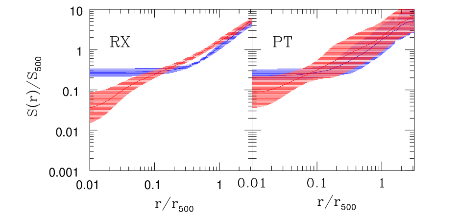
Figure 1: Ensemble averaged final radial entropy profiles are shown for the relaxed (perturbed) subsample in the left (right) panel. In each panel the entropy profile of the adiabatic (cooling) runs is shown in blue (red). The solid lines are the medians and the shaded areas represent the limit of the $1\sigma$ dispersion. The gas entropy is defined as $S(r)=k_{B}T(r)/n_{e}^{2/3}$ and is plotted in units of $S_{500}\simeq 1963\left[M_{500}/(10^{15}h^{-1}\rm{\,M_{\odot}})\right]^{2/3}keVcm^{2}$.

Application of the Beck et al. (2016b) SPH shock finder to the simulations leads to the identifications of shocks and to the assignement of individual Mach number $M_{i}$ to SPH particles. Shocks identified in this way will be used in some cases to apply a shock limiting procedure to the TH multifilter algorithm described in Sect. 4.2. The procedure is implemented as follows. For a given particle $i$ and filtering scale $H^{n}$ at the iteration level $n$, we stop the iteration if there are within the set of cells $\{\vec{q}\}_{i}^{n}$ some particles $s$ for which their Mach number $M_{s}$ is above a certain threshold value $M_{thr}$. We remove these particles, together with their neighbors, from the cells and define the filtering length $H_{i}^{n}$ as the minimum distance between $\vec{x}_{i}$ and the remaining particles $j$ in the cells: $H_{i}=\underset{j\in\vec{q}}{MIN}|\vec{x}_{i}-\vec{x}_{j}|$.

This shock limiting procedure leads to non-shocks filtering lengths $H_{i}^{\{ns\}}$ which are then smaller than their counterparts $H_{i}$, obtained without shock masking.

The choice of the threshold parameter $M_{thr}$ is a critical issue since the amount of reduction in the filtering lengths $H_{i}^{\{ns\}}$, due to the shock limiting procedure, depends on the value of $M_{thr}$. One has to distinguish between weak shocks ( say $M\sim 1$), which can be present in turbulent motions, and strong shocks ($M\lower 2.15277pt\hbox{$\;\buildrel>\over{\sim}\;$}1$) which occur in cluster outskirts, or during merging events, and act as sources of turbulence. As a compromise, and also for comparative purposes, as in Vazza et al. (2017) we set here $M_{thr}=1.2$.

5 Results

We now apply the statistical methods presented in Sect. 4 to the ICM velocity fields extracted from subsamples of simulated galaxy clusters, the analyses being aimed at studying their turbulent statistical properties. For each subsample we extract statistical results arising from considering velocity fields obtained by applying different filtering methods.

5.1 Global turbulence statistic from cluster subsamples

As outlined in Sect. 3, we perform our statistical analyses by constructing two subsamples out of the ensemble of simulated clusters, the subsample membership criterion for the simulated clusters being their dynamical status. This is identified through the value of the power ratio $\bar{\Pi}_{3}(r_{500})$ at $r=r_{500}$. Other choices of dynamical indicators are clearly possible (Rasia et al., 2013), but the power ratios are a commonly employed reliable and robust method (Weißmann et al., 2013).

The relaxed subsample (RX) is defined by those clusters for which their $\bar{\Pi}_{3}$ values are below the threshold value $\bar{\Pi}^{th}_{3}\simeq-8$, representing the $25\%$ of the cumulative distribution $N_{cl}(<\bar{\Pi}_{3})$. Similarly, for the perturbed clusters the subsample PT is defined by those clusters filling the top $25\%$ ($\bar{\Pi}_{3}>\bar{\Pi}^{th}_{3}\simeq-6$) of the $N_{cl}(<\bar{\Pi}_{3})$ distribution.

The threshold values $\bar{\Pi}^{th}_{3}$ are chosen with the compromise criteria of having subsample clusters with a well defined cluster dynamical status and, at the same time, subsample sizes ($N_{cl}\simeq 50)$ large enough to allow statistically meaningful comparisons.

In order to assess how realistic the simulations are which we use, for the two subsamples we show in Figure 1 the averaged radial entropy profiles. In each panel we show separately the profiles from adiabatic and radiative simulations. The shaded areas delimit one standard deviation of the subsamples.

We define as entropy the commonly employed related quantity $S\equiv k_{B}T/n_{e}^{2/3}$, where $T$ is the gas temperature and $n_{e}$ the electron density. To allow comparisons with previous results, in the plots we show $S(r)$ normalized to $S_{500}$. The latter is generically defined according to the self-similar model as (Nagai et al., 2007b)

$$S_{\Delta} \simeq 3070keVcm^{2}\left(\frac{M_{\Delta}}{10^{15}\rm{\,M_{\odot}}h^{-1}}\right)^{2/3}$$

$$(\Delta f_{b}^{2})^{-1/3}E(z)^{-2/3}h^{-4/3},$$ (39)

where $\Delta=500$, $f_{b}=\Omega_{b}/\Omega_{m}=0.162$ is here the cosmological baryon fraction, and for the mean molecular weights we assume $\mu=0.59~{},\mu_{e}=1.14$.

These entropy profiles can be compared with previous findings (Rasia et al., 2015; Barnes et al., 2017; Hahn et al., 2017). For instance, a comparison with Figure 1 of Rasia et al. (2015) shows substantial agreement with the radiative entropy profiles shown here. In their paper, the authors subdivide the sample of simulated clusters into cool-core (CC) and non-cool-core (NCC) clusters. Observationally, CC clusters are characterized by a dense, cold, compact core with a cooling time $t_{cr}$ shorter than $H_{0}^{-1}$. A key feature of these clusters is that of being associated with a regular X-ray morphology. On the contrary, for NCC clusters a specific feature is an high level of central entropy and a nearly flat core entropy profile. These are often associated with a disturbed morphology.

Various criteria have been proposed to classify CC clusters (Cavagnolo et al., 2009; McDonald et al., 2013); among these there is the requirement of having a central entropy $S_{0}$ below a threshold value: $S_{0}<60KeVcm^{2}$. This criterion is also used in Rasia et al. (2015) to identify simulated CC clusters. For the cooling runs of the RX subsample, only $4$ clusters out of $\simeq 50$ have a central entropy $S_{0}$ above the threshold value. These results confirm the use of a morphological criterion as a CC indicator, as well as the validity of the simulations presented here.

5.1.1 Filtering lengths

We have applied the multifiltering methods described in Sect. 4.2 to the ensemble of simulated clusters, in order to extract different sets of filtered velocity fields. For each filtering procedure, the radial behavior at the final epoch of the averaged root filtering lengths $<H(r)>$ is shown separately in Figure 2 for each cluster subsample. We show there only averages extracted from adiabatic simulations, the $<H(r)>$ profiles of the cooling runs being quite similar. All of the averaged lengths have been rescaled in units of $r_{200}$; the different curves are labeled according to Table 2. The ensemble average power spectra of the corresponding filtered velocity fields are shown in Figs. 3 to 5.

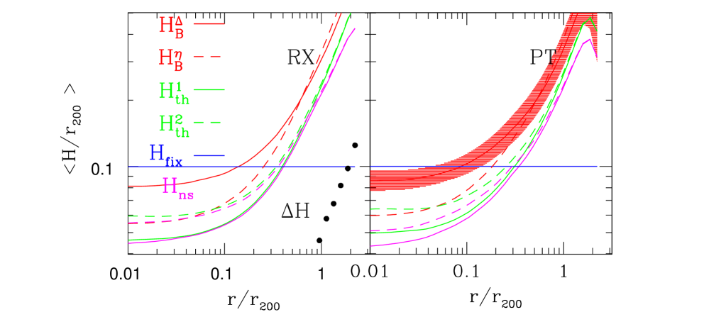
Figure 2: Average radial profiles of the turbulent filtering scales $H(r)$ are shown at $z=0$ as a function of $r$ in units of $r_{200}$. The left panel refers to averaged lengths extracted from the relaxed (RX) subsample of adiabatic simulations, the right panel to the perturbed (PT) one. Different color-codings and line styles indicate curves obtained according to the different procedures described in Sect. 4.2. The line in blue (${H_{fix}}$) refers to the TSC filtering, for which we use a fixed filtering length ${{H_{fix}}}=r_{200}/10$. The curves in magenta ($H_{ns}$) refer to the corresponding $H_{th}$ curves in green, but are obtained by applying the shock-masking procedure of Sect. 4.3. For illustrative purposes, in the right panel the shaded area indicates the limit of the $1\sigma$ dispersion of the $H^{\Delta}_{B}$ curve. The black circles in the left panel show the relative difference $\Delta H/r_{200}=(H_{th}-H_{th}$(HR)$)/r_{200}$ between two TH profiles extracted from the same test cluster. The profile $H_{th}$ refers to the baseline run and $H_{th}$(HR) to a high resolution run (see text).

The radial dependence of the different $<H(r)>$ profiles depends on a number of issues related to the adopted procedure. In the case of B-spline filtering the behavior of $<H^{\Delta}_{B}(r)>$ is different from that of $<H^{\eta}_{B}(r)>$. Specifically, from the left panel of Figure 2 one sees that the ratio $<H^{\Delta}_{B}(r)>/<H^{\eta}_{B}(r)>$ is $\lower 2.15277pt\hbox{$\;\buildrel>\over{\sim}\;$}1$ for $r/r_{200}\lower 2.15277pt\hbox{$\;\buildrel<\over{\sim}\;$}0.8$ and becomes smaller than unity at larger radii.

This behavior can be understood in terms of the different root finding methods adopted by the two procedures. In both methods the $H^{0}_{i}$ are initially set to $\zeta h_{i}$, however their increment $\Delta H$ at each iteration is different. The increment ratio between the $\Delta H$ of the two methods is given by $r_{H}(r)=\Delta H^{\Delta}_{B}/\Delta H^{\eta}_{B}=f_{H}r_{200}/(\eta\zeta h_{i}(r))\propto\rho^{1/3}$, so that it tends to higher values with decreasing radii. For the chosen root finding parameters, $r_{H}(0)\simeq 4$, with $r_{H}(r)\lower 2.15277pt\hbox{$\;\buildrel<\over{\sim}\;$}1$ at large radii because of the drop in density. The corresponding ratio between the root lengths is $H^{\Delta}_{B}/H^{\eta}_{B}\simeq(1+\eta r_{H})/(1+\eta)$, so that $H^{\Delta}_{B}$ is about $30\%$ higher than $H^{\eta}_{B}$ in the cluster cores.

These results show how the set of root values $\{H_{i}\}$ found using the multifilter method depends critically on the set of chosen initial values $H_{i}^{0}$ as well as on the step lengths $\Delta H$. In the $H_{B}$ cases, both methods start by setting $H^{0}=\zeta h_{i}$, and because in cluster cores the velocity field is very regular, the root values $\{H_{i}\}$ are found at the second iteration. The difference between the roots is then given by the different increments $\Delta H$ used in the two procedures.

We now examine the radial behavior of the TH filtering lengths. At variance with B-spline filtering, here we set the initial grid spacing to a very small value $H^{0}=\zeta h_{i}^{MIN}$. This guarantees that root finding starts from mesh values $H$ safely below those of the generic root. For the same reason we set the grid increment to very small values : $\Delta H=f_{H}r_{200}$ , with $f_{H}=1/200$. From Figure 2 one can see that the average value of the root set $H^{1}_{th}$ is very close to that of $H^{\eta}_{B}$ for $r/r_{200}\lower 2.15277pt\hbox{$\;\buildrel<\over{\sim}\;$}0.1$. This occurs because the small increments in grid spacing ensure that the root values are bracketed without overstepping, whilst for the same reason the $H^{\Delta}_{B}$ are found biased toward high values.

Note that in Figure 2 the $H_{B}$ profiles have been rescaled by a factor of two with respect the corresponding root values; this is because according to the definitions of Sect. 4.2 the $H_{B}$ root is a radius, while for TH filtering the root length is the grid size.

The averaged profile of the $H^{2}_{th}$ roots is quite similar to that of $H^{1}_{th}$. This is not surprising since for the filtering procedure of $H^{2}_{th}$ the search radius is twice that of $H^{1}_{th}$, but the very small value of $\Delta H$ implies that the two procedures converge to the same root. In the following parts of this paper, this filtering case will not be discussed any more, and we will refer only to $H^{1}_{th}$.

For the TH filtering, we have also applied the shock limiting procedure described in Sect. 4.3 to extract from the simulated samples a set of roots $H^{(ns)}_{th}$. As discussed in Sect. 4.3, the application of a shock limiter leads to filtering lengths $H^{(ns)}_{th}$ smaller than or equal to their counterpart $H_{th}$. The average radial profile $H^{(ns)}_{th}$ depicted in Figure 2 shows at small radii ($r\lower 2.15277pt\hbox{$\;\buildrel<\over{\sim}\;$}r_{200}$) a behavior very close to that of the unmasked filtering lengths $H_{th}$. Beyond $r_{200}$ the $H^{(ns)}_{th}$ begins to drop low, because of accretion shocks present in the cluster outskirts. We thus expect for relaxed clusters at late epochs the effects of masking to be negligible for $r\lower 2.15277pt\hbox{$\;\buildrel<\over{\sim}\;$}r_{200}$.

For the perturbed clusters the average radial profiles are displayed in the right panel of Figure 2. These profiles have been extracted by applying the same filter procedures used for relaxed clusters. The radial dependence of the profiles is the same as for the RX subsample, but the dispersion is higher. For the sake of clarity in one case ($H^{\Delta}_{B}$), we show the area delimiting the one sigma dispersion.

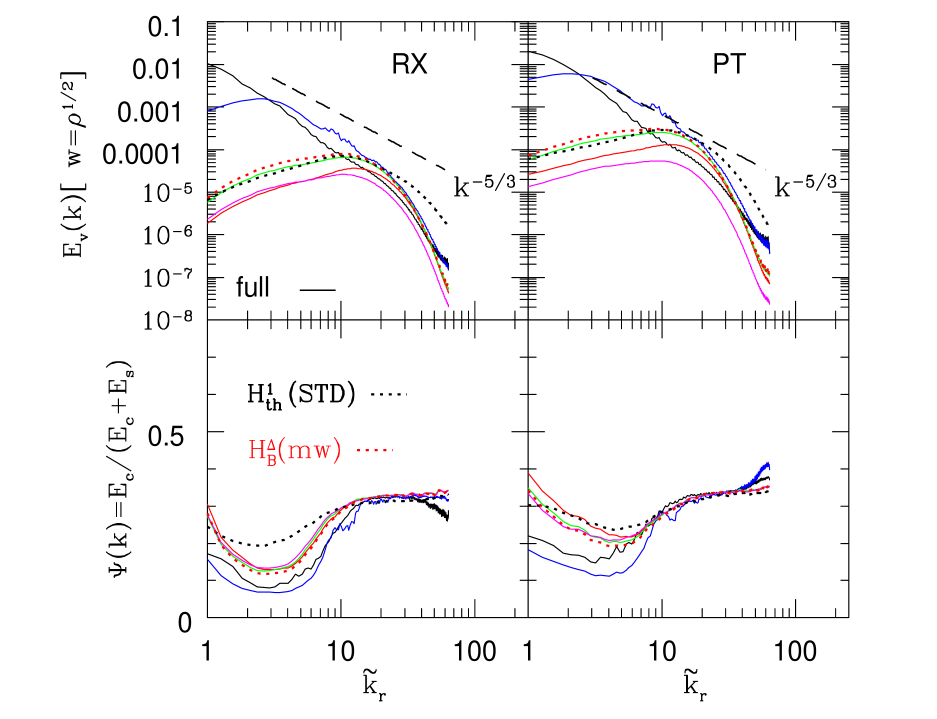
Figure 3: The ensemble averaged density-weighted velocity power spectra $E_{v}=E_{s}(k)+E_{c}(k)$ are shown in the top panels as functions of the dimensionless wavenumber ${\tilde{k}}_{r}\equiv kL_{sp}/2\pi$, where $k=|\vec{k}|$. The spectra are extracted from the adiabatic cluster simulations at $z=0$ using a cube of size $L_{sp}=r_{200}$ with $N_{g}^{3}=128^{3}$ grid points and are shown up to the wavenumber ${\tilde{k}}=N_{g}/2$. The left (right) panel refers to averages obtained from the relaxed (perturbed) subsample RX (PT), see text. In each panel the line style and color-coding is the same as in Figure 2. The spectra are normalized according to Equation (25). The solid black line shows the spectrum of the full (unfiltered) velocity field, whilst the dashed black line indicates the Kolgomorov scaling. The black dotted line $H_{th}(STD)$ refers to the spectra filtered according to $H^{1}_{th}$, but extracted from standard SPH runs. The red dotted line is for spectra extracted from velocities filtered using the $H_{B}^{\Delta}$ prescription, but mass-weighted (see text). The bottom panels show the ratio of the longitudinal to total velocity power spectra for the same spectra shown in the bottom panels.

At $r\lower 2.15277pt\hbox{$\;\buildrel>\over{\sim}\;$}r_{200}$, the filtering lengths show evidence of some degree of decrease as the radius increases. This indicates that the outskirts of some clusters of the PT subsample are dynamically unrelaxed, with perturbed velocity flows.

To demonstrate that the $H(r)$ profiles presented here are not affected by numerical resolution, for a single test cluster we show in the left panel of Figure 2 the relative difference $\Delta H/r_{200}$ between two distinct TH profiles $H_{th}$. This is a highly relaxed cluster whose properties are discussed in great detail in Sect. 5.2. To assess the effects of numerical resolution, for this test cluster we extracted the profile $H_{th}$(HR) from a high resolution run (HR). This was performed by running a simulation with about twice the number of particles of the baseline run. We then contrast in Figure 2 (black circles) the difference $\Delta H=H_{th}-H_{th}$(HR) between the baseline and HR profile. The results indicate a relative difference $\Delta H/r_{200}\lower 2.15277pt\hbox{$\;\buildrel<\over{\sim}\;$}4\cdot 10^{-2}$ at radii $r\lower 2.15277pt\hbox{$\;\buildrel<\over{\sim}\;$}r_{200}$, thus validating the effectiveness of the adopted numerical resolution for the baseline runs.

For the same test cluster, we obtain in Sect. 5.2 similar results when discussing the dependency of the velocity power spectrum on numerical resolution. We argue in Sect. 5.2 that the weak resolution dependency of the ISPH scheme, when compared against standard SPH, is a consequence of its ability to suppress gradient errors. In the standard SPH formulation these errors are strongly affected by numerical resolution, so that in the new scheme resolution dependency is now subdominant (Valdarnini, 2016).

Finally, it is important to emphasize that the applicability of the multifilter method requires a well defined separation between the coherence scale of bulk flows and that of small-scale motions. This in order to allow a proper definition of a local mean field. This condition might not be fulfilled in the case of cluster mergers, for which the largest injection scales of turbulence could approach that of large scale motions.

To validate their method, Vazza et al. (2012) analysed turbulent velocity fields extracted from a set of idealized test cases. In particular, for cluster mergers the spectral behavior of the ICM velocity field is found to be dominated by turbulent motions at spatial scales $r\lower 2.15277pt\hbox{$\;\buildrel<\over{\sim}\;$}0.1-0.3r_{200}$. At larger scales the motion is mostly laminar. This is in accord with the results presented in the next Section and supports the use of the multifiltering approach to detect turbulent motions in the ICM.

5.1.2 Power spectra and velocity structures (adiabatic simulations)

Velocity power spectra obtained by applying the different filtering procedures to the simulated cluster velocities are shown in Figures 3-5. Their behavior exhibits differences which can be interpreted in terms of the variations among the $<H(r)>$ profiles discussed in the previous Section. Additionally, we also show (solid black line) the power spectra of the unfiltered velocity fields.

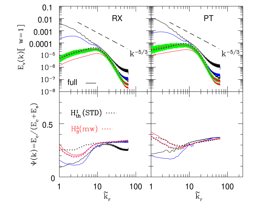
Figure 4: As in Figure 3, but spectra are volume weighted. The green areas in the top panels represent the $1\sigma$ dispersion range of the averaged power spectra, filtered according to the $H^{1}_{th}$ procedure.

The density-weighted spectra of the adiabatic simulations (Figure 3) are characterized by a peak at ${\tilde{k}}\sim 10-20$ and a power-law behavior $E(k)\propto k^{\alpha}$ at higher wavenumbers, with a slope $\alpha\simeq-2$, steeper than Kolgomorov scaling ($E(k)\propto k^{-5/3}$). These results are in agreement with previous findings (Vazza et al., 2012, V11), and indicate how ICM motion becomes turbulent at spatial scales $r\lower 2.15277pt\hbox{$\;\buildrel<\over{\sim}\;$}0.1-0.3r_{200}$.

The slope $\alpha$ shows some evidence of being steeper than in the unweighted case (Figure 4). This difference is interpreted as being due to the excess power detected at ${\tilde{k}}\sim 10$ by the density weighting scheme. The peaks in the power spectra are common both to relaxed and unrelaxed clusters, with a higher amplitude in the PT case due to a greater occurrence of merger events.

These features of the power spectra of adiabatic runs are shared also by the unweighted spectra of Figure 4 and can be considered statistically robust, given the size of the subsamples, suggesting the following scenario. At cluster scales ${\tilde{k}}\lower 2.15277pt\hbox{$\;\buildrel<\over{\sim}\;$}1-2$, the ICM motion is dominated by accretion flows from large scales, whereas at small scales turbulent motion is driven by hydrodynamic instabilities generated by substructure motion and merging events (Takizawa, 2005; Subramanian et al., 2006).

The spectral behavior of the filtered spectra exhibits differences which are worth investigating in order to assess the advantages and shortcomings of the adopted filtering methods. For a constant filtering scale, application of the filtering procedure (31) removes from the small-scale velocity field $\tilde{\vec{u}}_{k}$ the spectral components defined by the condition $kH\lower 2.15277pt\hbox{$\;\buildrel<\over{\sim}\;$}1$. One thus expects the spectral content of $\tilde{\vec{u}}_{k}$ at small wavenumbers to be further reduced as $H\rightarrow 0$.

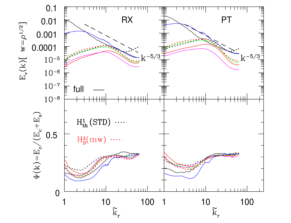
Figure 5: As in Figure 3, but for the cooling runs.

At large scales the power spectra ${E_{fix}}(k)$ extracted from the fixed filtering length set, show a decrease as $\tilde{k}\lower 2.15277pt\hbox{$\;\buildrel<\over{\sim}\;$}3$. This is consistent with simple analytical estimates, for which the condition $k{H_{fix}}\lower 2.15277pt\hbox{$\;\buildrel<\over{\sim}\;$}1$ is equivalent to $\tilde{k}\lower 2.15277pt\hbox{$\;\buildrel<\over{\sim}\;$}10/2\pi$.

Similarly, at large scales the spectra ${E_{fix}}$ are well above the spectra of all of the other filtering methods which we use. This is clearly a failure of the fixed length approach, as can be seen from Figure 2: at $r\lower 2.15277pt\hbox{$\;\buildrel<\over{\sim}\;$}0.2-0.5r_{200}$ one has either ${H_{fix}}>H_{th}$ or ${H_{fix}}>H_{B}$ which leads the corresponding spectra to approach the unfiltered case. This was already noticed by Vazza et al. (2012), for whom the agreement between the fixed filtering length and multifiltering becomes worse at cluster scales. This discrepancy is due to the coexistence at large scales of both laminar infall and chaotic motion, with the fixed filtering method missing the velocity correlations.

As one can see from Figure 2, application of the shock masking procedure to the $H^{1}_{th}$ filtering leads to profiles $H^{(ns)}_{th}(r)$ which are quite close to the unmasked one : $H^{(ns)}_{th}(r)\sim H^{1}_{th}(r)$ , at least for $r\lower 2.15277pt\hbox{$\;\buildrel<\over{\sim}\;$}r_{200}$. This is at odds with what seen in Figure 3, where the amplitude of the corresponding power spectra $E_{th}^{ns}(k)$ (solid magenta) is systematically smaller than that of the unmasked case $E_{th}(k)$ (solid green).

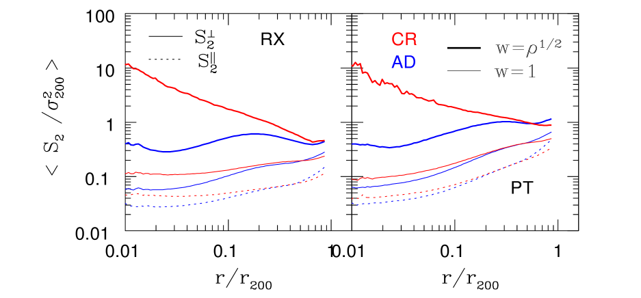
Figure 6: The ensemble averaged second-order longitudinal and transverse velocity structure functions are shown at $z=0$ as a function of $r/r_{200}$. The left (right) panel refers to the relaxed (perturbed) subsample. In each panel the profiles extracted from adiabatic (cooling) runs are shown in blue (red). The thick solid lines show the transverse density-weighted velocity structure functions.

This difference in power spectra is due to the weighting scheme used to evaluate $E(k)$. If the spectra are density-weighted as in Figure 3, then application of a shock limiter preferentially removes from filtering averages the high density particles. This is confirmed by Figure 4, where the spectra are volume-weighted and the two power spectra $E_{th}^{ns}(k)$ and $E_{th}(k)$ sit on top of each other.

Similarly, differences between spectra $E_{B}(k)$ extracted from $H_{B}$ filtering must be interpreted as being due to a weighting effect. From Equation (36) we have seen that evaluation of the filtered velocity (29) is equivalent to a convolution with a Gaussian, with similar half-width if the smoothing kernel radii satisfy the equalities (35).

From Figure 2, one has $H_{B}(r)\lower 2.15277pt\hbox{$\;\buildrel>\over{\sim}\;$}H_{th}(r)$ and for the corresponding spectra in Figure 3 (solid red) this would imply $E_{B}(k)\lower 2.15277pt\hbox{$\;\buildrel>\over{\sim}\;$}E_{th}(k)$. This is not verified, in fact Figure 3 shows spectra derived from $H_{B}$ filtering that are below those extracted from the TH filters. We argue that this behavior can be explained by differences in the adopted weighting scheme.

In the TH case, we set the filter function to $G(|\vec{x}_{i}-\vec{x}_{j}|,H_{i}^{n})=m_{j}$, so that the velocity $\bar{\vec{v}_{i}}^{n}$ in Equation (31) is a mass-weighted average. In the B-spline filtering procedure $G(|\vec{x}_{i}-\vec{x}_{j}|,H_{i}^{n})=m_{j}W_{ij}(H^{n}_{i}/\zeta)$, which is the SPH density estimate of particle $j$ at point $\vec{x}_{i}$. In this case velocity averages are density-weighted and the particles $j$ nearest to particle $i$ are weighted more.

One can regard this smoothing procedure as equivalent to a TH smoothing but with an effective radius $<H_{B}$ which, accordingly, leads to final spectra $E_{B}(k)$ smaller than in the mass-weighted case. To verify this conclusion, we constructed a set of filtering lengths $H_{B}(mw)$ by setting $G=m_{j}$ and computed the corresponding power spectra. These are shown in Figures 3 to 5 ( red dots) and consistently follow the spectra $E_{th}(k)$.

In order to assess the accuracy of the numerical method which we use, we have applied the TH filtering to an ensemble of clusters simulated using a standard SPH code. The corresponding power spectra are shown in Figures 3 to 5 and are indicated as $H_{th}(STD)$ (black dots). Their spectral behavior demonstrates that the use of a higher-order method, such as ISPH, is crucial at small-scales in order to ensure an accurate modeling of turbulence.

The density-weighted spectra of Figure 3, for standard SPH show excess power at high wavenumbers which is absent in the ISPH runs. This power arises from zeroth-order errors which are intrinsic to standard SPH, and in turn impact the modeling of vorticity. Similarly, at small wavenumbers, the longitudinal-to-total ratio $\Psi(k)\equiv E_{c}(k)/(E_{c}(k)+E_{s}(k))$ (Figure 3, bottom left) is higher than in the ISPH runs. This shows that the problem of properly accounting for the solenoidal part of the spectrum is not a resolution issue. In a previous paper (V11), it was argued that numerical resolution is critical when describing the solenoidal part $E_{s}(k)$ of the velocity power spectrum. The results presented here demonstrate that another key role is played by the numerical method adopted.

These discussions on the behavior of power spectra can be considered of general nature provided that the wavenumber dependency of an averaged spectrum is common to the corresponding power spectra of all the subsample clusters. This in turn implies that at each wavenumber the variance of an averaged power spectrum must be sufficient small. Here, the term sufficient is intended to mean that the area enclosing the $1\sigma$ power spectrum dispersion should retain the same spectral behavior exhibited by the averaged spectrum.

To confirm the correctness of our conclusions, for the volume-weighted power spectra $E_{th}(k)$ we then show in the top panels of Figure 4 the areas enclosing the one sigma dispersion around the means. As can be seen from the Figure, at each wavenumber the depicted range of power spectrum values is relatively small. This justifies the general character of our conclusions on the spectral behavior of the considered power spectra.

The wavenumber dependency of the ratio $\Psi(k)$ shows that ICM turbulent velocities are mostly solenoidal at large scales $\tilde{k}\lower 2.15277pt\hbox{$\;\buildrel<\over{\sim}\;$}10$, whilst at smaller wavenumbers the compressive component rises to $\Psi(k)\simeq 0.3-0.4$. We interpret this as a genuine feature of the measured spectra, and not as being due to a resolution effect (V11). The bending in $\Psi(k)$ occurs at approximately the same wavenumbers which characterize the maxima of the filtered power spectra. This is indicative of how turbulent motion at small scales is sourced by substructure motion and merging events, with small-scale shocks raising the compressive component of the velocity power spectrum.

Differences among the $\Psi(k)$ referring to different filtering methods, can be interpreted in terms of the differences between the corresponding power spectra. In particular, for TH filtering the behavior of $\Psi(k)$ is in agreement with previous results (see, Figure 8 of Vazza et al., 2017).

To summarize, the identification of the correct filtering strategy to be applied to the ICM velocity field depends critically on a number of issues. Numerically, the starting root $H^{0}$, as well as the search step $\Delta H$, should be chosen to be as small as possible in order to avoid possible biases in the final root values when in the presence of velocity fields with complex patterns.

Finally, the results presented here show that another critical feature is in the way in which the velocities in Equation (31) are weighted, rather than in the choice of the filtering function itself. This ambiguity is somewhat characteristic of turbulence and the choice of velocity weighting contains a degree of arbitrariness, which depends on the problem under consideration. As we will see in the next Sections, the top-hat filtering with mass-weighted velocities ($H^{1}_{th}$) seems to produce the most robust and unambiguous results.

In addition to spectral analysis, the second-order velocity structure function $\mathcal{S}_{2}(\vec{r})\propto r^{\gamma}$ provides information in physical space about the small-scale velocity field self-correlation. For homogeneous isotropic turbulence one has $\mathcal{S}_{2}(\vec{r})\propto r^{\zeta_{2}}$, with $\zeta_{2}=2/3$.

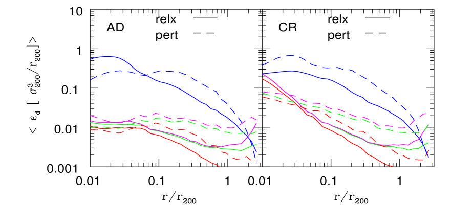
Figure 7: Average radial profiles of the turbulent dissipation rates $\varepsilon_{d}=\delta v^{3}/l$ , are shown at $z=0$ for adiabatic ( radiative) simulations in the left (right) panel. Solid (dashed) lines are for the relaxed ( perturbed) subsample. The color-coding indicates the adopted filtering as in Figure 2 : $H_{B}^{\Delta}$ (red), $H_{th}^{1}$ (green), ${H_{fix}}$ (blue), $H_{th}^{1}(ns)$ (magenta). The rates are in units of $\sigma^{3}_{200}/r_{200}$.

For the two cluster subsamples we show separately in Figure 6 the parallel and transverse second-order velocity structure functions. These are computed by using both volume-weighted and density-weighted velocities. All of the volume-weighted functions increase with increasing radii following a power-law behavior, with a slope significantly shallower than $\zeta_{2}$ for relaxed clusters and approaching $\zeta_{2}$ if one considers perturbed clusters. Similarly, the amplitude ratio of the transverse to longitudinal structure functions ( $S_{2}^{\perp}\simeq 2S_{2}^{\|}$) is almost constant in radii over two decades and higher ( $1+\zeta_{2}/2=4/3$) than that expected in the case of homogeneous isotropic turbulence.

The radial behavior of the structure functions can be compared with previous works (Miniati, 2014, 2015; Vazza et al., 2017). There is a general agreement, see for example Figure 7 of Vazza et al. (2017), but with some differences. Specifically, for the RX subsample we do not find any indication of a steepening at large scales in the longitudinal component. This is not verified for PT clusters, for which there is a hint for such a trend at radii approaching $r_{200}$. We interpret this as a consequence of the presence of shocks in the outskirts of unrelaxed clusters, which are absent form relaxed ones.

However we stress that making a proper comparison of statistical properties is difficult because the results presented here refer to sample averages performed over a large ($\simeq 50$) number of clusters, while in previous papers results were extracted by analyzing individual clusters.

Density-weighted structure functions exhibit a much shallower radial behavior than the volume-weighted functions. This was already noticed (V11) and it is a consequence of a selection effect. By using a density-weighted scheme, most of the contribution to the evaluation of the structure functions comes from high-density particles, which are located in the inner regions of the cluster. Because SPH is a Lagrangian code, these are the regions where the bulk of the particles are located.

5.1.3 Power spectra and velocity structures (radiative simulations)

We now repeat the analysis of the previous Section by applying the filtering methods to cluster velocities extracted from the ensemble of radiative simulations. As outlined in Section 2.4, the physical modeling of the gas then includes radiative cooling and star formation, as well as energy and metal feedback from supernovae (Piffaretti & Valdarnini, 2008).

We show in Figure 5 the density-weighted power spectra for the cooling runs. From a comparison with the corresponding spectra of Figure 3 for the adiabatic runs, it emerges that the spectral behavior of these spectra is characterized by a power excess at small scales. This feature was already noticed in V11, but the size of the samples allows it to be put now on a more robust footing.

This increase at small scales in the amplitude of the velocity power spectra is common both to relaxed and unrelaxed clusters, so that it can be assumed to be a general feature of realistic simulations of galaxy clusters which incorporate radiative cooling.

The differences in the spectra extracted using different filtering methods mirror those seen in the adiabatic case and will not be discussed further here. Similarly, we do not show here the volume-weighted spectra. These have a spectral behavior similar to the density-weighted ones, but with less exacerbated features. For these spectra, the slope at ${\tilde{k}}\lower 2.15277pt\hbox{$\;\buildrel>\over{\sim}\;$}10-20$ is close to ${\alpha}\lower 2.15277pt\hbox{$\;\buildrel<\over{\sim}\;$}-2$.

It is interesting to note how, for cooling runs, standard SPH badly fails to properly describe the velocity power spectra at high wavenumbers ($\tilde{k}\lower 2.15277pt\hbox{$\;\buildrel>\over{\sim}\;$}40$). These are characterized by a much higher amplitude ( $\sim 5$) than their ISPH counterparts. This is a clear shortcoming of the standard method, for which the magnitude of gradient errors translates into a difficulty in modeling turbulent motion at small scales and, in turn, produces noisier spectra. These discrepancies between the two methods will be further discussed in Sect. 5.2, and strengthen the view that the use of ISPH is crucial in order to ensure a proper modeling of turbulence in SPH simulations of galaxy clusters.

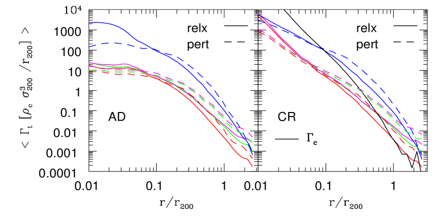
Figure 8: Normalized radial profiles of the turbulent heating rates $\Gamma_{t}=\rho_{g}\delta v^{3}/l$ are shown for the same filtering procedures and simulations as displayed in Figure 7. In the right panel, the solid black line indicates the average cooling rate profile $\Gamma_{c}=n_{e}n_{I}\Lambda(T)$ of the relaxed clusters.

We interpret (V11) the power excess seen at small scales in the spectra of Figure 5 as originating from the development of a dense, compact, gas core in the central region of the cluster. For cooling clusters, central gas densities are as high as $\rho/\rho_{c}\sim 10^{4}$, and are about a factor $\sim 10$ higher than in the corresponding adiabatic runs.

Interaction of compact cores with local gas motion triggers instabilities (Fujita et al., 2004; Dennis & Chandran, 2005; ZuHone et al., 2010; Banerjee & Sharma, 2014), which in turn generate turbulence. That the source of the power excess is due to the presence of a dense core is confirmed by the radial behavior of the density-weighted velocity structure functions $\mathcal{S}_{2}(\vec{r})$ (Figure 6), which for both relaxed and unrelaxed cooling clusters display a radial dependence decreasing with radius. Volume-weighted structure functions exhibit a very shallow slope $\gamma$, consistent with spectral findings ($\gamma\sim-(\alpha+2)$, ZuHone et al., 2016)

These results present a scenario in which turbulence in galaxy clusters is a multiscale phenomenon. The velocity power spectrum has a peak at wavenumbers corresponding to length scales $r_{200}/10\sim 100-300~{}kpc$, and this is the injection scale which drives turbulence through merging and substructure motion. The turbulent motion at large scales is mostly solenoidal.

At small scales there is the second injection mechanism, in which gas is stirred through the interaction of the medium with the core. This is the gas sloshing scenario, in which turbulent heating of the ICM has been proposed as a viable mechanism to offset radiative cooling (Fujita et al., 2004; Dennis & Chandran, 2005; ZuHone et al., 2010). Between these two scales one has subsonic turbulence in a compressible medium, but with a power spectrum having a slope which is found to be close to or steeper than that of Burgers turbulence ($\alpha=-2$).

To study the physics of turbulence in galaxy clusters, several authors (Yoo & Cho, 2014; ZuHone et al., 2016) have constructed mock observations of second order structure functions in the presence of multiple energy injection scales. Yoo & Cho (2014) argue that the ability to distinguish the injection scales in the projected functions depends critically on the relative heights of the peaks, as well as on the spatial separation between the injection scales.

The construction of mock X-ray maps of gas velocities and related 2D structure functions is a non trivial task, which is beyond the scope of this paper. Here we just note that the volume-weighted structure functions displayed in Figure 6 can be considered as being a realistic expectation of what can be measured from observations. See, for example, the similarity with the projected structure functions for the two-injection scale model shown in Figure 13b of ZuHone et al. (2016).

5.1.4 Turbulence related profiles

We now investigate the radial behavior of some ensemble averaged quantities which can be useful metric indicators for turbulence.

For the same filtering procedures previously considered, we first evaluate the turbulent dissipation rates $<\varepsilon_{d}(r)>$. Sample averages are computed by constructing individual cluster profiles $\varepsilon_{d}(r)\simeq\delta v^{3}/l$. These are obtained at each test radius by introducing a spherical shell with $40\times 40$ grid points $\vec{x}_{g}$, uniformly spaced in $\cos\theta,\phi$. We then compute at each grid point $\vec{x}_{g}$ the small-scale velocity field $\delta\vec{v}(\vec{x}_{g})$ and filtering lengths $l(\vec{x}_{g})$, estimated from individual particle values according to SPH prescriptions. Spherical averaged quantities $\delta v(r)$ and $l(r)$ are then defined by averaging over the grid points. The average radial profiles of other quantities are constructed according to the same procedure.

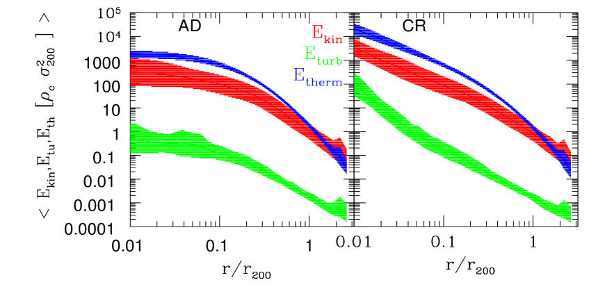
Figure 9: Final energy density radial profiles extracted from the relaxed subsample.The left panel is for adiabatic runs and the right panel is for cooling runs. In each panel are shown: the profile of the thermal energy density $E_{th}={3k_{B}T(r)\rho_{g}(r)}/{2\mu m_{p}}$, the kinetic energy density profile $E_{kin}=\rho_{g}\vec{v}^{2}/2$ and the turbulent one $E_{turb}=\rho_{g}{\delta v}^{2}/2$; the turbulent velocity field refers to TH filtering. The profiles have been rescaled in units of $\rho_{c}\sigma_{200}^{2}$, shaded areas represent the $1\sigma$ dispersion range.

The turbulent dissipation rate $\varepsilon_{d}(r)\simeq\delta v^{3}/l$, and subsequently the turbulent heating rate $\Gamma_{t}(r)\simeq\rho_{g}(r)\varepsilon_{d}(r)$, can be considered as being robust indicators of turbulence (Vazza et al., 2017). In the Kolgomorov scaling regime one has $\delta v\propto l^{1/3}$, so that $\varepsilon_{d}$ should be scale independent. We have seen in the previous Section that estimated power spectra do not follow Kolgomorov scaling in the inertial range. ($\propto k^{-5/3}$). Nevertheless, $\varepsilon_{d}(r)$ is still a very useful quantity, since its radial behavior provides spatial informations about the energy budget of turbulence, as well as about its deviation from the Kolgomorov regime.

For some of the adopted filtering strategies, we show the corresponding averaged profiles $<\varepsilon_{d}(r)>$ in Figure 7. The left panel is for adiabatic simulations and the right panel is for cooling runs. Within each panel, solid ( dashed) lines are for the $\varepsilon_{d}(r)$’s referring to relaxed (perturbed) subsamples. To consistently perform averages between clusters , the cluster values of $\varepsilon_{d}(r)$ have been rescaled to dimensionless units: $\varepsilon_{d}\rightarrow\varepsilon_{d}r_{200}/\sigma_{200}^{3}$. A first result to be inferred from Figure 7 is that the fixed length scale method grossly overestimates the dissipation rates. This is not surprising, given the spectral results already discussed.

For adiabatic simulations, there is some hint of Kolgomorov scaling only in the case of unrelaxed clusters. For these clusters $<\varepsilon_{d}>$ stays nearly constant over a radial range of about two orders of magnitude. This is verified only for the $\varepsilon_{d}$’s extracted from $H^{1}_{th}$ filtering, and with the related shock-limiting procedure $H^{1}_{th}(ns)$. Over the same range of scales, the condition $\varepsilon_{d}\simeq const$ is not sustained by the rates corresponding to the $H^{\Delta}_{B}$ procedure. This is a failure of this filtering method, and illustrates how root finding and weighting schemes can introduce biases in the final root filtering length values.

For relaxed clusters the condition $\varepsilon_{d}\simeq const$ holds to a lesser extent, with $\varepsilon_{d}(H^{1}_{th})$ dropping from $\varepsilon_{d}\simeq 8\cdot 10^{-3}$ at $r=10^{-2}r_{200}$ down to $\varepsilon_{d}\simeq 2\cdot 10^{-3}$ at $r\simeq r_{200}$. This deviation from Kolgomorov scaling arises because the corresponding power spectra are steeper than in the unrelaxed case. We suggest that this is a natural condition for turbulence in a steady-state ICM, with the excess power sourced by merging activity bringing the spectra to approach the Kolgomorov scaling.

The dissipative rates $\varepsilon_{d}[H_{th}(ns)]$, obtained by applying shock masking to the filtering procedure, begin to deviate and become higher than in the unmasked case at $r\lower 2.15277pt\hbox{$\;\buildrel>\over{\sim}\;$}r_{200}$. This result holds for both relaxed and unrelaxed cases, independently of weather one is considering adiabatic or radiative simulations. We have verified that it is not due to a resolution effect, by running a high resolution simulation for a individual cluster (Sect. 5.2). The dissipative rates extracted from the simulated clusters were compared with the corresponding ones from the standard run, obtaining very similar values.

Our results then indicate that at large radii $r\lower 2.15277pt\hbox{$\;\buildrel>\over{\sim}\;$}r_{200}$, dissipative rates tend to be underestimated if the filtering estimator is applied without a shock limiter. At these radii, application of a shock limiter is mostly effective, since the presence of supersonic inflows due to accretion shocks is significative, and leads to filtering lengths $H_{ns}$ smaller than $H_{th}$ (Sect. 5.1.1). From previous results concerning velocity structure functions (Sect. 5.1.2), we have seen that $\delta v\propto l^{\beta}$, with $\beta>0$ being some value less than unity. Therefore, this implies $\varepsilon_{d}[H_{th}(ns)]>\varepsilon_{d}[H_{th}]$ as $l_{ns}<l_{th}$.

The dissipative rates of the cooling runs are shown in the right panel of Figure 7. In contrast to the profiles extracted from adiabatic simulations, here the profiles exhibit a steady rise when approaching the cluster center. This raise is particularly steep in the case of relaxed clusters, and is consistent with the findings of Sect. 5.1.3. Accordingly, in the inner regions of cluster cooling runs, turbulence is sourced by the interaction of the ICM with high density cores, the latter being due to radiative cooling and the subsequent star formation.

To assess in a more quantitative way the impact of radiative cooling on turbulence, we look at the turbulent heating rate profiles $\Gamma_{t}=\rho_{g}\delta v^{3}/l$. These are constructed in the same way as the dissipation rates, we show in Figure 8 the profiles $\Gamma_{t}(r)$ corresponding to the rates of Figure 7.

For adiabatic simulations, the profiles $\Gamma_{t}(r)$ tend to approach constant values at small radii, when $r\rightarrow 0$. This is in contrast with the behavior of the corresponding profiles $\Gamma_{t}(r)$ extracted from the cooling runs. The profiles exhibit an approximate power-law dependency $\Gamma_{t}(r)\propto r^{-\gamma}$, with $\gamma>0$, spanning almost two orders of magnitude in radius, from $r\simeq 0.01r_{200}$ up to $r\simeq r_{200}$. The profiles are steeper for relaxed clusters than for unrelaxed ones, with $\gamma\simeq 3$ in the former case.

A crucial issue is to determine whether or not dissipation by turbulent heating can balance radiative losses in cluster cores. This possibility has been proposed by a number of authors (Fujita et al., 2004; Dennis & Chandran, 2005; ZuHone et al., 2010; Banerjee & Sharma, 2014; Zhuravleva et al., 2014a) as a viable mechanism to solve the cooling flow problem. For comparative purposes, we have evaluated for the simulated clusters of the relaxed subsample, the average radial profile of the gas cooling rate: $\Gamma_{c}=n_{e}n_{I}\Lambda(Z,T)$, where $\Lambda(Z,T)$ is the gas cooling function (Voit, 2005). These are evaluated at the radial bin from those of the individual particle temperatures and metallicities: $T_{i},~{}Z_{i}$.

The results indicate that the cooling rate $\Gamma_{c}$ is systematically higher than the turbulent heating rate $\Gamma_{t}$ at all radii for which $r\lower 2.15277pt\hbox{$\;\buildrel<\over{\sim}\;$}0.5r_{200}$. Basically, this is a consequence of the smallness of the turbulent velocity field $\delta v(l)$ in comparison to the other quantities which enter into the thermal energy budget of the cluster cores. This is confirmed by looking at the energy density radial profiles. These have been computed for the relaxed subsamples of the adiabatic and radiative simulations, the corresponding averages are shown in Figure 9.

Figure 10: Average final radial profile of the vorticity volume filling factor $f_{\omega}$ is shown in the right panel for the relaxed subsample of the cooling simulations. The shaded area represents the limit of the $1\sigma$ dispersion. The right panel shows the averaged final radial profiles of the enstrophy $\epsilon=\omega^{2}/2$ for the relaxed subsamples of the adiabiatic (blue) and cooling (red) simulations. For clarity, the shaded area representing the $1\sigma$ dispersion is shown only for the cooling runs.

In each panel are plotted the radial profiles of the the kinetic energy density $E_{kin}=\rho_{g}\vec{v}^{2}/2$, the thermal energy density $E_{th}={3k_{B}T(r)\rho_{g}(r)}/{2\mu m_{p}}$, and the turbulent energy density $E_{turb}=\rho_{g}{\delta v}^{2}/2$. For the thermal energy $T(r)$ is the mass-weighted gas temperature, $k_{B}$ is the Boltzmann constant and $m_{p}$ is the proton mass; the turbulent velocity field $\delta v$ refers to the TH filtering.

From the profiles, one sees that the ratio $E_{turb}/E_{th}$ is always $\lower 2.15277pt\hbox{$\;\buildrel<\over{\sim}\;$}1\%$ across all the cluster radius. For the cooling runs, at $r\simeq 0.1r_{200}$ one even has $E_{turb}/E_{th}\simeq 10^{-4}$. This is in contrast with previous findings, see for example Figure 16 of V11. For the test clusters considered there, $E_{turb}/E_{th}\simeq 2-5\%$. This discrepancy is clearly due to the use of a multifiltering approach; in V11 a fixed filtering length was used for which we have seen (Sect. 5.1.2) that turbulent velocities can be significantly overestimated.

Given the importance of the topic, we defer discussion on this to the next Section. There, for a single highly-relaxed cluster we will study in detail the profiles of some turbulence related quantities.

From previous results on power spectra we have seen that turbulence in the ICM is dominated by solenoidal motion, which is characterized by the vorticity $\vec{\omega}=\vec{\nabla}\times\vec{v}$. A useful quantity used to quantify solenoidal turbulence is the vorticity magnitude, or enstrophy:

$$\epsilon=\frac{1}{2}\omega^{2}~{}.$$ (40)

In accord with previous studies (Miniati, 2014; Porter et al., 2015; Schmidt et al., 2016; Vazza et al., 2017; Iapichino et al., 2017; Wittor et al., 2017), we will use this quantity to obtain spatial information about the nature of ICM turbulence.

A complementary measure used to characterize turbulence is the volume filling factor. In mesh based codes, this is the volume fraction of the cells which satisfy the conditions $\omega_{i}>N/t_{age}(z)$, where $N$ is the number of eddy turnovers and is set to $N=10$ (Miniati, 2014; Iapichino et al., 2017). At the present epoch the condition becomes $\omega_{i}>NH_{0}$. In the SPH framework we then define the volume fraction $f_{\omega}$ as

$$f_{\omega}=\frac{\sum_{i}f_{i}V_{i}}{\sum_{i}V_{i}}$$ (41)

where $f_{i}=1$ if $\omega_{i}>NH_{0}$ and zero otherwise, $V_{i}={m_{i}}/\rho_{i}$ and $\omega_{i}$ is given by Equation 15. As for the dissipation rates, we obtain radial profiles $f_{\omega}(r)$ by doing spherical averages of (41) for the same set of radial bins.

We show $f_{\omega}(r)$ for the relaxed subsample of the cooling clusters in the left panel of Figure 10. We do not show the corresponding profile for unrelaxed clusters since its quite similar, but with a larger dispersion. The right panel of the Figure for the RX subsample shows the radial enstrophy profiles $\epsilon(r)$ extracted from adiabatic and radiative simulated clusters. Averages were performed by rescaling cluster enstrophies to dimensionless units : $\epsilon\rightarrow{\tilde{\epsilon}}=\epsilon(r_{200}/\sigma_{200})^{2}$.

We can see from Figure 10 that the volume filling factor of ICM turbulence is very high in the cluster inner regions, with $f_{\omega}(r)\lower 2.15277pt\hbox{$\;\buildrel>\over{\sim}\;$}95\%$ for $r\lower 2.15277pt\hbox{$\;\buildrel<\over{\sim}\;$}0.5r_{200}$. Beyond this radius $f_{\omega}(r)$ begins to steadily decrease, with $f_{\omega}(r)\simeq 80\%$ $r\simeq r_{200}$ and smaller values at larger radii.

These findings are in qualitative agreement with previous results (Miniati, 2014; Iapichino et al., 2017), see for example Figure 8 of Iapichino et al. (2017). However, we stress that making a quantitative comparison is difficult because we are presenting here averages extracted from cluster samples, whereas previous papers showed results from a single individual cluster.

As seen in the right panel of Figure 10, at small radii there are significant differences between the enstrophy profile $\epsilon(r)$ of cooling cluster simulations and the corresponding adiabatic one. This shows a flat profile for $r\lower 2.15277pt\hbox{$\;\buildrel<\over{\sim}\;$}0.1r_{200}$, while for the cooling runs, $\epsilon(r)$ exhibits a well defined power-law behavior over more than two decades in radius. This is clearly correlated with the presence of a much denser core in cooling clusters and is consistent with the findings of Sect. 5.1.3.

For relaxed cooling clusters, the power-law dependency of $\epsilon(r)$ is suggestive of some sort of self-similarity at work. From Kolgomorov scaling one has $\omega(l)\propto l^{-2/3}$, but we have seen from the analysis of Sect. 5.1.3 that velocity power spectra are steeper than $5/3$. We thus expect $\omega(l)$ to have a steeper dependency on the eddy size $l$. Nonetheless, it is still reasonable to assume a dependency of the kind $\omega(l)\propto l^{-\beta}$ with $\beta>0$. This then implies a regulating mechanism for $l$ which sets the eddy size at radius $r$; we argue that buoyancy forces due to the strength of gravity can be this mechanism. We will discuss this point in more detail in Sect. 5.2.

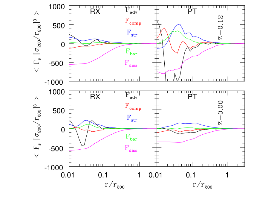
Figure 11: Averaged radial profiles of the different source and sink terms present in the enstrophy evolution equation are shown for the relaxed ( perturbed) subsample of the adiabatic runs in the left (right) panels. The top panels refer to averages evaluated at $z=0.12$ and bottom panels to $z=0$.

To investigate the different processes leading to the generation and diffusion of solenoidal turbulence, it is also useful to look at the enstrophy time evolution equation, this can be written as follows (Porter et al., 2015)

$$\frac{d\epsilon}{dt}=F_{adv}+F_{stretch}+F_{comp}+F_{baroc}+F_{diss}~{},$$ (42)

with the source and sink terms on the rhs of the equation given by

$$\left\{\begin{aligned} F_{adv}&=&-\vec{\nabla}\cdot(\vec{u}\epsilon)=-(\epsilon\cdot\vec{\nabla}\vec{u}+\vec{u}\cdot\vec{\nabla}\epsilon)~{},\\ F_{stretch}&=&\vec{\omega}\cdot(\vec{\omega}\cdot\vec{\nabla})\vec{u}=2\epsilon(\vec{\hat{\omega}}\cdot\vec{\nabla})\vec{u}\cdot\vec{\hat{\omega}}~{},\\ F_{comp}&=&-\epsilon\vec{\nabla}\cdot\vec{u}=-\vec{\nabla}\cdot(\vec{u}\epsilon)+\vec{u}\cdot\vec{\nabla}\epsilon~{},\\ F_{baroc}&=&\frac{\vec{\omega}}{\rho^{2}}\cdot(\vec{\nabla}\rho\times\vec{\nabla}P)~{},\\ F_{diss}&=&\nu\vec{\omega}\cdot(\nabla^{2}\vec{\omega}+\vec{\nabla}\times\vec{G})~{},\end{aligned}\right.$$ (43)

where $\vec{G}=\frac{1}{\rho}\vec{\nabla}\rho\cdot\vec{S}$, with $\vec{S}$ being the traceless strain tensor (Porter et al., 2015); a hat denotes a unit vector and $\nu$ is the numerical kinematic viscosity. For the latter we adopt the SPH estimate $\nu_{i}\simeq\alpha_{i}c_{i}h_{i}/10$ (Price, 2012a). The only source term able to generate vorticity is the baroclinic term, aside from dissipative effects, the other terms describing the processes of advection, compression and stretching. SPH estimates of the different terms (43) are computed at a given test point $\vec{x}_{g}$ from individual particle values. Radial profiles are then obtained according to the same procedure as previously described.

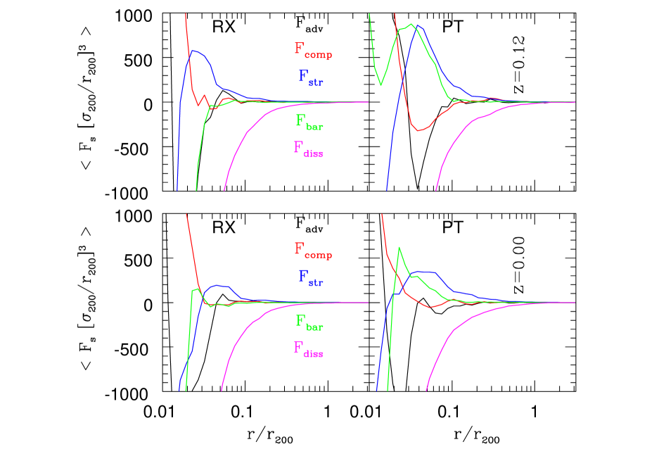
Figure 12: As in Figure 11, but for the cooling runs.

Previous studies (Porter et al., 2015; Vazza et al., 2017; Wittor et al., 2017) have investigated, for individual clusters, the time evolution of the volume averages of the source and sink terms present in Equation (42). Here we present ensemble average radial profiles at two different time slices. Figure 11 shows, for adiabatic simulations, the mean profiles of the terms (43), obtained by averaging individual cluster profiles, at the times $z=0.12$ (upper panels) and $z=0$ (bottom panels). The left panels refer to profiles extracted from the RX subsample, the right panels are for the PT subsample.

Profiles extracted from the PT subsample show the impact of the baroclinic, stretching and compression terms as enstrophy generators, with the baroclinic term being the primary source. All of these terms make a non-negligible contribution to enstrophy production, see for example Figure 11 of Wittor et al. (2017). Relaxed clusters are instead characterized, as expected, by smaller amplitudes than the PT profiles.

The most important aspects of the impact of the driving terms (43) on enstrophy evolution have already been investigated in some detail (Vazza et al., 2017; Wittor et al., 2017). We focus here on the differences between the profiles extracted from adiabatic simulations and the corresponding profiles computed from radiative runs; these are depicted in Figure 12.

Source term profiles of the cooling runs are characterized by higher amplitudes, however the most pronounced differences are seen at small radii $r\lower 2.15277pt\hbox{$\;\buildrel<\over{\sim}\;$}0.1r_{200}$. Whilst at $z=0$ adiabatic profiles of the different terms (43) exhibit the tendency to approach zero or small values (with the exception of $F_{diss}$, but see later); in the same radial range, cooling run profiles tend to increase/decrease to large values.

This is clearly a consequence for the cooling runs of the development of large gas densities in gas cores, which in turn imply a steep rise of the compressive term $F_{comp}$ towards the cluster center, with the other terms now acting as sink terms. To assess the robustness of the results against numerical resolution, for a single individual cluster we ran a high resolution simulation (Sect. 5.2) with an higher number of particles. We found the final enstrophy profile to be almost identical to that of the standard resolution run (Figure 13), and so conclude that the profiles depicted in Figures 11 and 12 are not adversely affected by resolution effects.

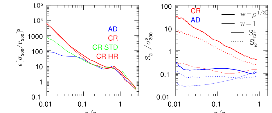
Figure 13: The final enstrophy profiles of the highly relaxed cluster with sample index $cl=133$ are shown in the left panel for several simulations: adiabatic (AD, blue), cooling (CR, red), with cooling but the simulation run using standard SPH (CR STD, green), with cooling but with a simulation performed using an higher resolution ( $N^{HR}_{p}\simeq 2N_{p}$, CR HR magenta). For the same cluster, the right panel shows the radial behavior of the second-order longitudinal and transverse velocity structure functions. Results from the adiabatic (cooling) run are shown in blue (red). The thick lines show the density-weighted velocity structure functions. For clarity, in the unweighted case, only the transverse velocity structure functions are shown.

We have verified that the average profile $\epsilon(r)$ of relaxed clusters is nearly stationary since $z\lower 2.15277pt\hbox{$\;\buildrel<\over{\sim}\;$}0.5$. This suggests that, at least for relaxed clusters, at late times a condition of equilibrium is reached with the different terms (43) balancing each other and giving $d\epsilon/dt\simeq 0$.

The very large (negative) values of the dissipative term $F_{diss}$ require some explanation. This term accounts for numerical viscosity effects and in Eulerian codes it is difficult to estimate its impact (Wittor et al., 2017), since there is no explicit expression for the viscosity $\nu$. Here, for particle $i$ we estimate $F_{diss}(i)$ by setting the viscosity parameter to $\nu_{i}\simeq\alpha_{i}c_{i}h_{i}/10$ (Price, 2012a). This choice is commonly used to estimate the amount of numerical viscosity in SPH simulations (see, for example, Price, 2012b).

However, it is worth noting that the contribution of particle $j$ to the AV tensor (18) of particle $i$ is applied only when the two particles are approaching. This means that by setting $\nu_{i}\simeq\alpha_{i}c_{i}h_{i}/10$ one puts an upper limit to the effective AV viscosity of particle $i$. We thus conclude that using this estimator in an equilibrium configuration, such as that present in cluster inner regions, leads to a dissipative term $F_{diss}$ which is likely to be overestimated. The stationarity of the profile $\epsilon(r)$ appears then to be driven by the physical terms present in Equation (42).

5.2 An individual study of a very relaxed cluster

To better investigate the impact of turbulence on the properties of cool-core clusters, we have decided to look carefully at the behavior of some turbulence related quantities for a single individual cluster extracted from the relaxed subsample of the cooling runs, the cluster selection criterion being that of having at $z=0$ the lowest subsample value of $\bar{\Pi}_{3}(r_{500})$. This is $\bar{\Pi}_{3}(r_{500})\simeq-9.4$ and the cluster has sample index $cl=133$. By definition this is also the most relaxed cluster of the whole sample.

The smallness of the moment $P_{3}$ indicates that this cluster, for all practical purposes, can be considered perfectly spherical. We thus expect to gain some insights about the impact of turbulence in cluster cores, the cluster being in a well defined highly relaxed state. Note that it would not have been possible to identify such a cluster without a very large sample size ($\simeq 200$ clusters). For $\Delta=200$, the cluster mass (24) is $M_{200}\simeq 1.04\cdot 10^{14}\rm{\,M_{\odot}}h^{-1}$, so that $r_{200}\simeq 1.1Mpc$ and $\sigma_{200}\simeq 770kmsec^{-1}$.

We first show in Figure 13 the profiles of the final enstrophy (left panel) and the velocity structure function (right panel) of the chosen cluster. To check the validity of the simulation results, in the left panel of Figure 13 we show the enstrophy profiles extracted from several additional runs. In particular, we tested the numerical convergence of the $\epsilon^{cr}(r)$ profile by running a simulation with a higher number of particles (HR), about as twice as many as in the baseline run, with the other simulation parameters being rescaled accordingly. We indicate the corresponding enstrophy profile as $\epsilon^{HR}(r)$. We also show the profile $\epsilon^{ad}(r)$ extracted from the adiabatic simulation, and the $\epsilon^{STD}(r)$ profile of the standard SPH run.

There are several conclusions to be drawn from the radial behavior of the profiles depicted in the left panel of Figure 13. The first is that $\epsilon^{HR}(r)\simeq\epsilon^{cr}(r)$ throughout all of the radial range probed by the plots. This confirms that the numerical resolution which we use is adequate to properly describe the properties of turbulence in the ICM of galaxy clusters.

Secondly, the profile of $\epsilon^{STD}(r)$ begins to deviate from $\epsilon^{cr}(r)$ at radii $r\lower 2.15277pt\hbox{$\;\buildrel<\over{\sim}\;$}0.1r_{200}$ and at $r\simeq 0.01r_{200}$ it is smaller than $\epsilon^{cr}(r)$ by almost one order of magnitude. This is consistent with previous findings (Sect. 5.1.2) and happens because the impact of gradient errors is much larger in standard SPH than in ISPH. This in turn implies, for the standard code, a noisier description of vorticity and smaller amplitudes of $\omega(r)$ at small scales. This clearly demonstrates for SPH simulations of galaxy clusters, the importance of using ISPH in the modeling of turbulence.

The adiabatic profile $\epsilon^{ad}(r)$ is depicted for comparative purposes, from a comparison with the profiles in the right panel of Figure 10, we see that the central value of $\epsilon^{ad}(r)$ is close to the ensemble average value ($\simeq 10^{2}$). This is in contrast with the cooling run profile $\epsilon^{cr}(r)$, which has a central value higher by a factor $\simeq 10$ than the corresponding ensemble average. This suggests that the large value of the central density ($\rho_{g}/\rho_{c}\simeq 10^{5}$) is closely linked to the highly relaxed state of the cluster. It is also consistent with the proposed scenario, in which vorticity in the cluster inner regions is driven by the interaction of the ICM with the dense compact cores.

Similarly, for the cooling runs, the profiles of the second-order velocity structure functions (right panel of Figure 13) exhibit the same differences with respect the ensemble average profiles of Figure 6.

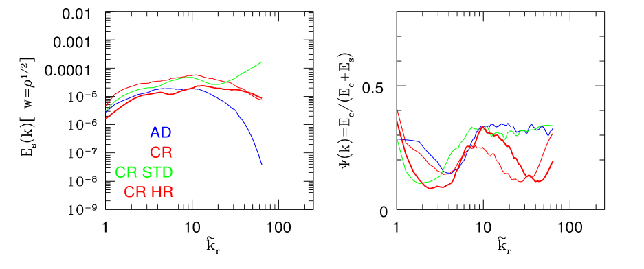
Figure 14: The left panel shows the wavenumber dependency of the shearing components of the density-weighted velocity power spectra for the same cluster simulations shown in the left panel of Figure 13. In the right panel are shown the corresponding ratios of the longitudinal to total velocity power spectra.

For the same test runs, we show in Figure 14 the density-weighted solenoidal velocity power spectra, together with the ratios $\Psi(k)\equiv E_{c}(k)/(E_{c}(k)+E_{s}(k))$. The spectral behavior of the spectra displayed in the left panel of Figure 14 is consistent with the findings about enstrophy profiles. The solenoidal spectra $E_{s}(k)$ and $E^{HR}_{s}(k)$ are nearly identical across all of the wavenumber range, whilst $E^{STD}_{s}(k)$ is characterized by a power excess at high wavenumbers ($\tilde{k}\lower 2.15277pt\hbox{$\;\buildrel>\over{\sim}\;$}40$). This is similar to what was already seen in the spectral behavior of the ensemble average spectra (Sect. 5.1.3).

The longitudinal-to-total ratio $\Psi(k)$ exhibits several features which are in contrast with the behavior of the corresponding ensemble averaged profile. The bottom-left panel of Figure 5 shows the ensemble averaged quantity $\Psi(k)\simeq 0.3$ at all the wavenumbers $\tilde{k}\lower 2.15277pt\hbox{$\;\buildrel>\over{\sim}\;$}10$.

On the contrary, from the right panel of Figure 14 we see that the longitudinal component is sub dominant ( $\Psi(k)\simeq 0.1$) in the range between $\tilde{k}\simeq 10$ and the highest wavenumber. This is also valid for the ratio $\Psi(k)$ of the high-resolution run. We interpret this discrepancy at high wavenumbers along the same line as the difference between the central value of the cluster cooling run enstrophy profile $\epsilon^{cr}(r)$ and the corresponding sample average value. For highly relaxed clusters, the large values of central densities act as drivers for the generation of vorticity, so that the solenoidal component of the power spectrum is dominant.

In order to assess the effects of numerical resolution on the results presented in this paper, for the test cluster considered here we show in Figures 13 and 14 profiles extracted form a high resolution (HR) run. The simulation was performed by running again the ISPH cluster simulation, but with a number of particles increased by a factor $\sim$ two. The profiles of the HR run are indicated in the Figures with CR HR, whereas the profiles corresponding to the standard resolution run are labeled as CR. From Figure 14 it can be seen that at all the wavenumbers the power spectrum extracted from the HR run almost coincides with the corresponding standard resolution one.

It is also worth noticing that this result is in stark contrast with previous findings ( see, e.g., Figure 9 of V11). In that paper it was argued that to properly describe velocity power spectra over a decade in wavenumbers, at least $N\lower 2.15277pt\hbox{$\;\buildrel>\over{\sim}\;$}256^{3}$ gas particles are necessary in standard SPH simulation of galaxy clusters.

As already noticed in Valdarnini (2016), this discrepancy follows because the ISPH scheme is highly effective in removing gradient errors, which are dominant at small scales. This in turn implies that ISPH simulations of subsonic turbulence exhibit at high wavenumbers velocity power spectra with a much weaker dependency on numerical resolution.

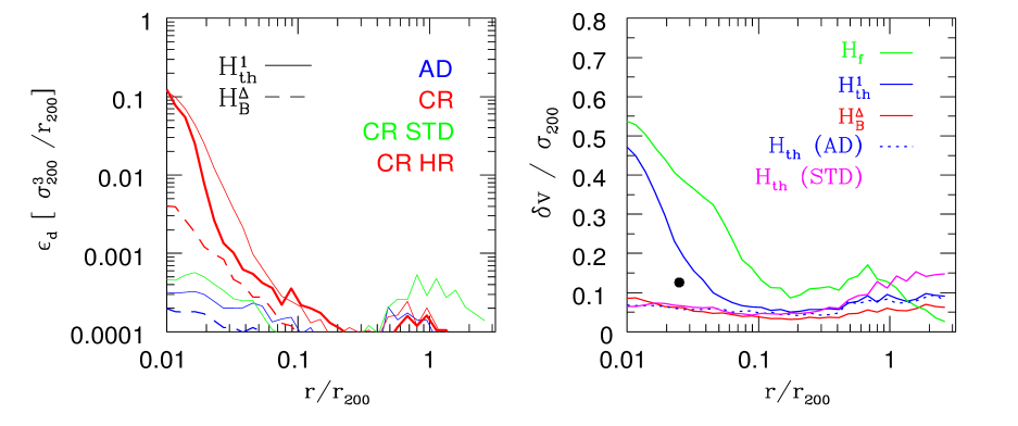
Figure 15: For the same set of cluster simulations depicted in Figure 13, turbulent dissipation rates $\epsilon_{d}$ are shown in the left panel. Different line styles indicate different filtering methods: solid ( dashed) lines refer to $H_{th}^{1}$ ($H_{B}^{\Delta}$). The radial behavior of different local turbulent velocity fields $\delta v$ (Equation 32) are shown in the right panel as obtained by applying different multifiltering procedures to the same cluster simulations as in Figure 13, the color coding of the curves is referenced by the corresponding labels. The black dot refers to the Hitomi velocity measurement in the Perseus core, rescaled in dimensionless units.

Finally the turbulent dissipation rates, extracted from the suite of simulations analyzed here, are shown in the left panel of Figure 15. We consider profiles obtained by applying to cluster velocities the $H_{th}$ and $H^{\Delta}_{B}$ filtering.

For TH filtering, the $\varepsilon_{d}(r)$ profile extracted from the high resolution run is very similar to the baseline profile. This again confirms the view that the results presented here can be considered numerically robust. Instead, the shortcomings of standard SPH previously discussed now translate into a failure to estimate the dissipation rates at small scales.

At small radii ($r\lower 2.15277pt\hbox{$\;\buildrel<\over{\sim}\;$}0.2r_{200}$), the rates obtained by applying $H^{\Delta}_{B}$ filtering severely underestimate the dissipation rates in cluster cores. This is a deficiency of the filtering strategy already discussed in Sect. 5.1.1, and indicates the $H_{th}$ filtering procedure as the optimal choice among the tested filtering methods.

The turbulent velocity profiles $\delta v(r)$ are shown in units of $\sigma_{200}$ in the right panel of Figure 15. The profile $\delta v^{(th)}(r)$ extracted from TH filtering exhibits a steep raise as one approaches small radial distances, with a central value as high as $\delta v^{(th)}/\sigma_{200}\simeq 0.5$. This behavior is shared by the small-scale velocity field $\delta v^{(f)}$ corresponding to the fixed length filtering, but with a higher amplitude. This is not surprising given the biases inherent in this approach.

Both profiles $\delta v(r)$ obtained either by applying $H^{\Delta}_{B}$ filtering or from the standard SPH run, are almost flat as a function of radius. This is in line with previous findings and the profiles of these runs will not be discussed further.

It is interesting to note that the profile $\delta v(r)$ of the adiabatic run, extracted by using TH filtering, is also characterized by a very flat behavior. This demonstrates that a realistic description of turbulence in cluster cores cannot be obtained without incorporating at least radiative cooling, and subsequently star formation and feedback processes, in the physical modeling of the gas. In summary, among the profiles depicted in the right panel of Figure 15, $\delta v^{(th)}(r)$ should represent most faithfully the radial behavior of turbulent velocities in a relaxed cluster.

To assess whether the turbulent velocity profile $\delta v^{(th)}(r)$ is realistic, we can compare it with observations. To this end we use the first direct detection of gas motion in galaxy clusters (H16). The observations measured, in the core of the Perseus cluster, a line-of-sight velocity dispersion of $164\pm 10~{}kms^{-1}$ in the region $30-60~{}kpc$ , and a gradient of $150\pm 70~{}kms^{-1}$ across the $60~{}kpc$ central region.

The Perseus cluster is a nearby ($z\simeq 0.0179$), relaxed massive object. Simionescu et al. (2011) report a cluster mass at $\Delta=200$ of $M_{200}\simeq 7\cdot 10^{14}\rm{\,M_{\odot}}$, with $r_{200}\simeq 1.8Mpc$. This implies $\sigma_{200}\simeq 1300kmsec^{-1}$. By rescaling the measured velocities one thus obtains $\delta v/\sigma_{200}\simeq 0.126$ at the midpoint radius $r/r_{200}\simeq 0.025$.

This value is smaller than the simulation value of $\delta v^{(th)}$ at the same radius: $\delta v^{(th)}/\sigma_{200}\simeq 0.2$, but is not grossly inconsistent with it, given the uncertainties involved in the comparison. In particular, our sample cluster is very relaxed but less massive ($M_{200}\simeq 1.04\cdot 10^{14}\rm{\,M_{\odot}}h^{-1}$) than Perseus. Our findings suggest that the presence of turbulence in cluster cores is closely linked to the impact of cooling and to the development of large core densities. Therefore, at a given radius one expects to measure a relative increase in the strength of turbulence as the cluster mass decreases.

Another quantity to be compared with simulation results is the ratio of kinetic to thermal energy density in the core. From measured velocities (H16) this ratio is found to lie in the range $\simeq 5-10\%$. This value is not in contrast with that obtained from the energy density profiles depicted in the right panel of Figure 9. At $r/r_{200}\simeq 0.05$ the ratio is estimated to be $E_{kin}/E_{th}\simeq 10\%$, broadly consistent with observations.

However, a critical issue to be kept in mind is that the simulations presented here are purely hydrodynamical, and do not include several physical processes which can impact on the modeling of turbulence in cluster cores. In particular, we do not incorporate AGN feedback. This is a severe limitation in the case of Perseus, because the cluster is observed to host a powerful AGN activity (Fabian et al., 2011) which is expected to drive turbulence in the cluster core (Zhuravleva et al., 2016).

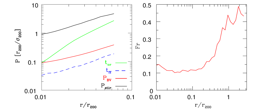
Figure 16: Left: For the cooling run of the highly relaxed cluster $cl=133$, several timescales are shown as a function of radius. The sloshing oscillation period $P_{BV}=2\pi/\omega_{BV}$, where $\omega_{BV}$ is the Brunt-Väisälä frequency, (solid red line); the stirring period $P_{stir}=2\pi/\omega_{stir}$, where $\omega_{stir}=\delta v/l$ , (solid black line); the cooling time $t_{cr}\simeq(3/2)nk_{B}T/Q_{R}$ (solid green line); the free -fall time $t_{ff}\simeq 1/\sqrt{\rho}$ (dashed blue line). Right: the radial behavior of the Froude number $Fr\simeq\delta v/(\omega_{BV}l)$.

Recently, a number of authors (Hiller & Socker, 2017; Lau et al., 2017; Bourne & Sijacki, 2017; ZuHone et al., 2018) have investigated the consistency of the low level of gas motion observed in the Perseus core with the presence of an on-going AGN activity. Simulation results have reached conflicting conclusions, in particular ZuHone et al. (2018) argue that gas sloshing alone is sufficient to reach the observed level of gas velocities. We will return on this topic in the Conclusions.

We now investigate the radial behavior of some characteristic timescales which regulate gas motion in the cluster center. In a medium at equilibrium having ${dlnS}/{dlnr}>0$, a fluid element displaced at the radius $r$ from its equilibrium position will be driven back by a restoring force and will oscillate at the the buoyancy or Brunt-Väisälä frequency (Cox, 1980)

$$\omega_{BV}=\Omega_{K}\sqrt{\frac{1}{\gamma}\frac{dlnS}{dlnr}}~{},$$ (44)

where $\Omega_{K}=\sqrt{GM/r^{3}}$ is the Keplerian frequency.

The ICM of a relaxed cluster exhibits density variations by more than three orders of magnitude across the whole cluster, and in a strongly stratified stable medium the impact of buoyancy forces on turbulence is significant. This hydrodynamical regime is well known in geophysical fluid mechanics (Riley & Lelong, 2000) and is commonly referred to as stratified turbulence.

To quantify the impact of gravity on turbulence it is convenient to introduce the Froude number (Riley & Lelong, 2000)

$$Fr\simeq\frac{\delta v}{\omega_{BV}l}~{},$$ (45)

which measures the relative importance of buoyancy forces in comparison to stirring motion. If $\it Fr\lower 2.15277pt\hbox{$\;\buildrel>\over{\sim}\;$}1$ inertial forces are dominant, while when $\it Fr\lower 2.15277pt\hbox{$\;\buildrel<\over{\sim}\;$}1$ the effect of stratification is significant.

In this regime the gas motion is preferentially tangential, being suppressed along the radial direction by buoyancy restoring forces. This follows because the stirring frequency is lower than the Brunt-Väisälä frequency : $\delta v/l\lower 2.15277pt\hbox{$\;\buildrel<\over{\sim}\;$}\omega_{BV}$ and gas motion excites gravity waves which are trapped inside the radius given by the condition ${\it Fr}\simeq 1$ (Ruszkowski & Oh, 2010; Zhuravleva et al., 2014b). The nature of these gravity waves, or g-modes, is found to be preferentially tangential (Cox, 1980; Lufkin et al., 1995; Riley & Lelong, 2000), and the regime $\it Fr\lower 2.15277pt\hbox{$\;\buildrel<\over{\sim}\;$}1$ is then characterized by anisotropic turbulence.

We have evaluated the radial profile of the gas sloshing period $P_{BV}(r)=2\pi/\omega_{BV}$ up to the maximum radius $r_{max}(S)\simeq 0.08r_{200}$ for which ${dlnS}/{dlnr}>0$. Note that, for the clusters of the relaxed subsample, the test cluster $cl=133$ is the one with the maximum value of $r_{max}(S)$. To construct the radial profile we have estimated $\alpha_{S}={dlnS}/{dlnr}$ by setting $\alpha_{S}=1.1$.

Additionally, we also evaluate the stirring motion timescale $P_{stir}=2\pi/\omega_{stir}\simeq 2\pi l/\delta v$, the cooling time scale $t_{cr}\simeq(3/2)nk_{B}T/Q_{R}$, and the the free -fall time $t_{ff}\simeq 1/\sqrt{\rho}$. All of these profiles are shown in the left panel of Figure 16; the Froude number $\it Fr(r)=P_{BV}(r)/P_{stir}(r)$ is depicted in the right panel.

A clear result which emerges from the plots is that in the probed radial range

$$t_{ff}<P_{BV}\lower 2.15277pt\hbox{$\;\buildrel<\over{\sim}\;$}t_{cr}<P_{stir}~{},$$ (46)

and there is a very weak stirring motion with a strongly stratified turbulence having $\it Fr\lower 2.15277pt\hbox{$\;\buildrel<\over{\sim}\;$}0.1$ up to $r\simeq 0.1r_{200}$.

This result is particularly important since it indicates that, in the inner regions of relaxed clusters, turbulence is dominated by buoyancy forces and regulated by the Brunt-Väisälä frequency. Recently Shi et al. (2018), from an adiabatic simulation of a single cluster, obtained similar values for the Froude number in the cluster inner high density region. Turbulent velocities were extracted by applying a wavelet analysis, so that their result provides an independent confirmation of our values for the Froude number.

The profiles of Figure 16 can be compared with recent measurements of the Fornax cluster (Su et al., 2017b). Fornax is a very close by $z\simeq 0.00475$ low mass cool core cluster, with approximately $r_{200}\simeq 750~{}kpc$ (Su et al., 2017a). Chandra observations reveal that the cluster morphology is typical of a sloshing cluster, with discontinuities in the X-ray surface brightness and multiple sloshing cold fronts (Su et al., 2017a).

From a combined Chandra and XMM-Newton analysis Su et al. (2017b) derive ICM density and temperature profiles. Under the assumption of hydrostatic equilibrium, these profiles were used to calculate the Brunt-Väisälä frequency and the sloshing period $P_{BV}$ at the radius $r$. In addition, they derived also the free-fall and cooling time scales. The radial behavior of these profiles in the cluster core are shown in their Figure 8, along the x-axis the radial distance $R=10~{}kpc$ corresponds to $r/r_{200}\simeq 0.01$.

A comparison with the corresponding profiles depicted here in the left panel of Figure 16 shows a remarkable agreement. The ratio $P_{BV}/t_{ff}$ is of the order of $P_{BV}/t_{ff}\simeq 5$ up to $r/r_{200}\simeq 0.04$.

From their Figure 8 for the dimensionless period at $R=10~{}kpc$ we obtain $P_{BV}/t_{200}\simeq 2\cdot 10^{2}/1.3\cdot 10^{3}\simeq 0.15$, where we have estimated for the Fornax cluster $t_{200}=r_{200}/\sigma_{200}\simeq 1.3\cdot 10^{3}Myr$. This is close to the value of $P_{BV}/t_{200}\simeq 0.1$ found here at $r/r_{200}\simeq 0.01$

The ratio $t_{cr}/P_{BV}$ is found here to decrease from the range $t_{cr}/P_{BV}\simeq 5-10$ above $r/r_{200}\lower 2.15277pt\hbox{$\;\buildrel>\over{\sim}\;$}0.02$ down to unity at $r/r_{200}=0.01$. This is in contrast with the measured ratio, for which $t_{cr}/P_{BV}\simeq 5-10$. This divergent behavior at small distances is not unexpected, given the absence in the simulations of AGN heating.

From the X-ray analysis of the Fornax cluster, Su et al. (2017b) argue that gas sloshing contributes to the heating of the core. Their conclusions are based on the smallness of the measured sloshing timescale with respect $t_{cr}$. The agreement between the timescale radial profiles extracted from our simulations, and the corresponding profiles shown in their Figure 8 supports this view. However, it is worth noting that over the probed radial range, the profiles of Figure 16 never violate the condition $t_{stir}>t_{cr}$. This implies a condition of negligible turbulent mixing and , in agreement with the findings of Sect. 5.1.3, that the contribution of sloshing motions to core heating is sub-dominant.

In the sloshing scenario, core heating proceeds via entropy mixing driven by the presence of KHI. The latter is identified in X-ray maps by the presence of KH eddies at the cold front interfaces (Markevitch & Vikhlinin, 2007). Since the growth of KHI is suppressed in the presence of a viscosity or an aligned magnetic field (ZuHone et al., 2011; Roediger et al., 2013), observational support for the presence of KH eddies (Su et al., 2017b, a) can then be used to put constraints on the ICM physical properties. The derived upper limits on the ICM Spitzer viscosity (Su et al., 2017b) favor an almost inviscid, weakly magnetized, ICM. This adds credibility to the use of the hydrodynamical simulations presented here in the modeling of ICM turbulence.

6 Summary and Conclusions

In this paper we have presented results concerning the properties of turbulent motions in the ICM. These have been identified by the application to cluster velocities of different multifiltering strategies, so as to separate bulk flows from small-scale motions. We have then applied these filtering procedures to gas velocities extracted from large sets of simulated clusters. The velocity power spectra and radial profiles of turbulence related quantities have then been contrasted to identify the optimal filtering strategy and to provide physical insights into the role of turbulence in the ICM. The application of different filtering methods to the same gas velocity sets, demonstrate that the root filtering lengths depends critically on a number of issues.

Numerically, it has been found that the values of the final root lengths $H_{i}^{n}$ are quite sensitive to the chosen initial values $H_{i}^{0}$ as well as to the step lengths $\Delta H$. This follows because the algorithm terminates the root search when Equation 33 is satisfied, thus the root values can be biased to high values if the interval bracketing the root is too large. This occurs in the presence of velocity fields with complex patterns, having short range correlations.

Similarly, the final root values $H_{i}^{n}$ are also determined by the choice of the filtering function $G(|\vec{x}|,H)$. We have adopted different smoothing functions to construct different sets of filtered velocities. The results of Sect. 5.1.1 and 5.1.2 demonstrate that differences in the corresponding velocity power spectra can be consistently interpreted in terms of the adopted smoothing procedures.

In particular, in comparison to TH filtering, B-spline smoothing tends to give more weight to close by particles. This in turn implies higher values for the root filtering lengths and lower amplitudes for the velocity power spectra. From the results presented in Sect.s 5.1.2 to 5.2, we argue that TH filtering represents, with the search parameters used here, the optimal choice to extract turbulent velocities in a variety of cluster dynamical states. In addition, note also that the fixed filtering length approach clearly fails in the presence of complex velocity flows.

Results extracted from subsamples of the adiabatic cluster simulation ensemble, delineate the following scenario for the generation and evolution of turbulence in the ICM. Power spectra of the small-scale filtered velocities exhibit a maximum at ${\tilde{k}}\sim 10-20$ and a power-law behavior $E(k)\propto k^{\alpha}$ at higher wavenumbers. The wavenumbers ${\tilde{k}}\sim 10-20$ correspond to the injection scales $r_{200}/10\sim 100-300~{}kpc$, with turbulence being driven by merging and substructure motion.

The slope ${\alpha}$ lies in the range ${\alpha}\simeq[-3,-2]$, with density weighted spectra being shallower than volume weighted ones. The turbulent motion at large scales is mostly solenoidal, with the fraction of longitudinal spectrum rising to $\simeq 0.3$ at small scales. Perturbed clusters are characterized by a power excess at small scales due to a higher merging rate. In fact, the slopes of their velocity power spectra are closer to Kolgomorov ($\alpha\simeq-5/3$), and the estimated dissipation rate $\varepsilon_{d}\simeq\delta v^{3}/l$ is nearly constant over the whole cluster radial range tested by the simulations ($\sim 0.01r_{200}$ to $\sim 2r_{200}$).

In this scenario the generation of vorticity proceeds initially through the baroclinic term, and is sustained by the compression and stretching terms present in the dissipative enstrophy Equation 43. These results are essentially in agreement with previous studies (Vazza et al., 2012, 2017; Iapichino et al., 2017; Wittor et al., 2017), the only substantial difference being the robustness of our findings given the size of the samples which we use.

For the cooling runs, the results of Sect. 5.1.3 to 5.2 demonstrate that ICM turbulence properties undergo a drastic change with respect those found in adiabatic simulations. This is due to the development of dense compact gas cores, as a consequence of radiative losses. These cores interact with the local gas motions triggering instability, and in turn leading to the development of turbulence (Fujita et al., 2004; ZuHone et al., 2010; Banerjee & Sharma, 2014).

When contrasted with adiabatic spectra, velocity power spectra of radiative runs are characterized by a much flatter wavenumber dependency. We interpret this as being due a consequence of the injection of turbulence at two different scales. The first injection is at scales $r_{200}/10\sim 100-300~{}kpc$, which drives turbulence through the usual mechanism. The second occurs at small scales and is due to the stirring of gas motions through interaction of the ambient medium with the core. This spectral behavior was already noticed in a previous paper (V11), but it is now statistically significant. The impact of these physical effects is important in several aspects.

The estimated dissipation rates $\varepsilon_{d}$ increase as $r$ decreases, with a very steep radial dependency in comparison to the adiabatic rates. In fact, the central values of $\varepsilon_{d}$ are higher by almost an order of magnitude. Nonetheless, the corresponding turbulent heating rates $\Gamma_{t}(r)=\rho_{g}\varepsilon_{d}$ are found to be unable to balance the cooling rates $\Gamma_{c}(r)$ in the cluster inner parts ($r\lower 2.15277pt\hbox{$\;\buildrel<\over{\sim}\;$}0.5r_{200}$ ). This calls into question the viability of the turbulent heating model (Zhuravleva et al., 2014a) for solving the cooling flow problem. This has already been noticed (Banerjee & Sharma, 2014), and is a consequence of the smallness of turbulent velocities in cluster cores.

Another striking feature that emerges from the analyses of the cooling runs is the behavior of the average radial enstrophy profile $\epsilon(r)=\omega^{2}/2$. For relaxed clusters the profile is stationary since $z\simeq 0.5$. and exhibits a power law dependency $\epsilon(r)\propto r^{-\beta}$, with $\beta\simeq 3/2$, over more than two decades in radius. Analysis of the enstrophy dissipation equation shows that the only source of enstrophy is the compression term, which is dominant as $r\rightarrow 0$ because of the large gas densities now present in cluster cores.

The power-law behavior of $\epsilon(r)$ implies a dependency of the vorticity amplitude on cluster radius $r$, which suggests that the eddy size $l$ also depends on radius: $l=l(r)$. To better clarify this issue we have investigated in detail the turbulence properties of a single, highly relaxed, cluster. In fact, the cluster has been chosen as being the most relaxed of the $\simeq 200$ sample clusters.

The cluster has sample index $cl=133$ and from the profiles displayed in Figure 15 we see that the turbulent dissipation rate and velocity profile have a very steep decline with radius. We have compared the turbulent velocity profile with the only available direct detection of gas motion in a galaxy cluster (H16). By rescaling the velocities measured in the core of the Perseus cluster we obtain at the estimated radius a dimensionless velocity which is $\sim 50\%$ smaller than the simulation value.

We do not consider this discrepancy as problematic, given the mass difference between Perseus and the simulated cluster as well as the non-linearities induced by cooling effects. However, the comparison confirms the low level of turbulent motions which we obtain in cluster cores. Note that, as previously outlined, it is the smoothing given by TH filtering which produces the velocity profile in best agreement with observational data.

We have also constructed the sloshing timescale profile and contrasted it with recent measurements presented for the Fornax cluster (Su et al., 2017b). In the probed radial range, from $0.01$ up to $0.05r_{200}$, we find that the sloshing oscillation period $P_{BV}(r)$ and other timescale profiles are in very good agreement with the measured timescales. Additionally, we used the profile $P_{BV}(r)$ to evaluate the Froude number, which is found to be $Fr\simeq\delta v/(\omega_{BV}l)\simeq 0.1$ up to $r\simeq 0.1r_{200}$.

We use this result, and the agreement with the Fornax cluster profiles, to draw several conclusions about the properties of turbulence in the cores of relaxed clusters. The smallness of the Froude number indicates that turbulent motion in cluster cores is dominated by gravitational buoyancy forces, with stirring motion strongly suppressed along the radial direction. In this regime of stratified turbulence, 2D stirring motions are very weak, and the energy injected is unable to sustain the cooling rate. We consider these findings as the main result of our paper.

The simulations presented here have a number of limitations which we discuss now. We have contrasted power spectra and turbulence related profiles against the corresponding ones extracted from clusters simulated using standard SPH. The results demonstrate the superiority of ISPH in the numerical modeling of subsonic turbulence. This is because it is crucial to keep gradient errors very small in order to ensure a correct description of vorticity (Valdarnini, 2016).

In particular, a previous paper (V11) argued for a strong dependence of solenoidal velocity spectra on numerical resolution and particle number. For the test cluster $cl=133$ we found numerical convergence (Figure 14) between the solenoidal velocity power spectra extracted from the baseline sample, and a high resolution run with about twice the number of particles. This demonstrates that the numerical resolution used here is adequate to describe velocity power spectra over more than a decade in wavenumber.

Whilst the numerical scheme which we use can be considered adequate to simulate ICM hydrodynamics, our physical modeling of the ICM is incomplete. Our baryonic physics incorporates radiative cooling, star formation and supernova feedback, but assumes an inviscid, unmagnetized, ICM. We consider these assumptions realistic, since X-ray observations of KHI (Su et al., 2017a, b) favor a low viscosity plasma with low values of ordered magnetic fields.

However, we do not include ICM heating due to AGN feedback. This model is widely supported both observationally and theoretically (see, for example, Zweibel et al., 2018, and references cited therein). In this scenario the ICM is thermalized by means of the interaction with buoyantly rising bubbles created from AGN jet activities. A variety of mechanisms have been proposed to transfer the feedback energy to the ICM (Zweibel et al., 2018), but it is still unclear which are the dominant processes driving the heat transport. In particular, Yang & Reynolds (2016b) argued, on the basis of purely hydrodynamical simulations, that turbulent heating from AGN feedback is negligible.

We conclude that our simulation results, which are consistent with available data, seem to rule out the turbulent heating model as the sole solution for the cooling flow problem. Similar conclusions have been recently reached by Mohapatra & Sharma (2018). From a set of homogenous isotropic turbulence simulations, which incorporate radiative cooling, the authors conclude that consistency with Hitomi results rules out turbulent heating models as the dominant source of heating in cool core clusters.

It then appears that the solution to this problem is highly non trivial, and will require galaxy cluster simulations of increasing physical complexity. In a Lagrangian framework, the adoption of ISPH is undoubtedly a step in the right direction.

Appendix A The shock detection algorithm

Following Beck et al. (2016b), shocks in SPH simulations are found as follows. When a shock front develops the local velocity exceeds the sound velocity, and the shock front separates the pre-shock (upstream) from the post-shock (downstream) regimes. The implementation of an SPH shock-finder requires first the identification of the shock direction and then the evaluation for particle $i$ of the hydrodynamic variables in the two regimes.

We identify for particle $i$ the direction of the shock normal $\vec{n}$ as given by the pressure gradient: $\vec{n}_{i}=-\vec{\nabla}P_{i}/P_{i}$, where

$$\vec{\nabla}P_{i}=\frac{1}{\rho_{i}}\sum_{j}m_{j}(P_{j}-P_{i})\vec{\nabla}W_{ij}$$ (A1)

is the SPH estimator for the pressure gradient (Price, 2012a). The normal $\vec{n}_{i}$ points in the downstream direction and the distances of the two regimes from particle $i$ are then $\vec{x}^{d,u}_{i}=\vec{x}_{i}\pm\zeta h_{i}\vec{n}_{i}$, where one is assuming that the shock extends throughout the kernel domain. Setting $\vec{x}_{i}-\vec{x}_{j}\equiv\vec{x}_{ij}$ downstream particles are identified by the condition $\vec{n}_{i}\cdot\vec{x}_{ij}>0$, whereas particles in the upstream regime satisfy $\vec{n}_{i}\cdot\vec{x}_{ij}<0$.

Hydrodynamic variables in the two states are evaluated by summing the contribution of the neighboring particles to the up- and downstream regimes. This is done by adopting a twofold weighting scheme. The first $(F)$ weights the particle $j$ according to its projected distance from the up- and downstream positions:

$$U^{F}_{ij}=\zeta-|\vec{n}_{i}\cdot\vec{x}_{ij}|/h_{i}~{}.$$ (A2)

The second $(S)$ weights the contribution of particle $j$ inversely with its distance from the shock normal:

$$U^{S}_{ij}=\sqrt{\vec{x}_{ij}^{2}-(\vec{n}_{i}\cdot\vec{x}_{ij})^{2}}/h_{i}~{}.$$ (A3)

An estimator of the hydrodynamic variables $Z=\{\rho,~{}P,~{}c_{s},~{}\vec{v}\}$ is then given by

$$Z^{s}_{i}=\frac{\sum_{j\in s}w_{ij}Z_{j}}{\sum_{j\in s}w_{ij}}~{},$$ (A4)

where $s=\{u,d\}$ is just a shorthand notation to indicate the two possible states and

$$w_{ij}=m^{2}_{j}W(U_{ij}^{F})W(U_{ij}^{S})$$ (A5)

is the total weight.

In order to compute the shock Mach number we must now apply the flux conservation laws between the up- and downstream hydrodynamic variables. However, unlike in Beck et al. (2016b), we allow here for the presence of bulk motions, such as those present in the cluster ICM.

We define the shock velocity in the lab frame to be $\vec{V}^{lab}_{sh}=V_{sh}\vec{n}_{sh}$, and in the shock rest frame the shock mass flux conservation is

$$\rho_{u}(\vec{V}_{u}\cdot\vec{n}_{sh})\equiv\rho_{u}V_{u}=\rho_{d}(\vec{V}_{d}\cdot\vec{n}_{sh})\equiv\rho_{d}V_{d}~{},$$ (A6)

where upstream and downstream velocities are measured in the shock rest frame. This equation in the lab frame is (Schwartz, 2000)

$$\rho_{u}(\vec{V}^{lab}_{u}-V^{lab}_{sh}\vec{n}_{sh})\cdot\vec{n}_{sh}=\rho_{d}(\vec{V}^{lab}_{d}-V^{lab}_{sh}\vec{n}_{sh})\cdot\vec{n}_{sh}~{},$$ (A7)

and the shock velocity in the lab frame is then the given by

$$V^{lab}_{sh}=\frac{\vec{n}_{sh}\cdot\Delta({\rho\vec{V}^{lab})}}{\Delta{\rho}}=\frac{(\rho_{d}V^{lab}_{d}-\rho_{u}V^{lab}_{u})}{\rho_{d}-\rho_{u}}~{}.$$ (A8)

We now define the particle Mach number $M_{i}$ as

$$M_{i}=\{V^{lab}_{sh}/c^{u}_{s}\}_{i},$$ (A9)

where we have used for particle $i$ the quantities previously derived from Equation (A4).

Finally, as in Beck et al. (2016b) , we apply a set of filterings criteria to avoid false detections and to reduce particle noise. We first require $P_{i}^{d}>(1+\epsilon)P_{i}^{u}$ and $\rho_{i}^{d}>(1+\epsilon)\rho_{i}^{u}$, where $\epsilon=0.05$. Moreover, the velocity divergence

$$\Delta v_{i}=\vec{n}_{sh}\cdot(\vec{V}_{d}-\vec{V}_{u})=V_{d}-V_{u}~{},$$ (A10)

must satisfy $\Delta v_{i}<0$ , since the shock compression ratio $r=\rho_{d}/\rho_{u}$ is greater than unity and from Equation (A6) one has $V_{d}<V_{u}$. Additionally, for the viscosity limiter $f_{i}={|\vec{\nabla}\cdot\vec{v}|_{i}}/{(|\vec{\nabla}\cdot\vec{v}|_{i}+|\vec{\nabla}\times\vec{v}|_{i})}$ we set a threshold value for $f_{i}>0.6$ to avoid false detections in shear flows. For all the gas particles we initialize $M_{i}$ to zero, so that only those particles which satisfy the filtering criteria have a non-zero Mach number.

References

- Adrian et al. (2000) Adrian, R.J., Christensen, K.T. & Liu, Z.C., 2000, Experiments in fluids, 29, 275
- Balsara (1995) Balsara, D., 1995, J. Comp. Phys., 121, 357
- Bambic et al. (2018) Bambic, C. J., Morsony, B. J. & Reynolds, C. S., 2018, ApJ, 857, 84
- Banerjee & Sharma (2014) Banerjee, N. & Sharma, P., 2014, MNRAS, 443, 687
- Barnes et al. (2017) Barnes, D. J., et al., 2017, MNRAS, 471, 1088
- Barnes et al. (2018) Barnes, D. J., et al., 2018, arXiv:1805.04109
- Battaglia at al. (2012) Battaglia, N., Bond, J. R., Pfrommer, C., & Sievers, J. L., 2012, ApJ, 758, 74
- Beck et al. (2016a) Beck, A. M., Murante, G., Arth, A., Remus, R.-S., Teklu, A. F., Donnert, J. M. F., Planelles, S., Beck, M. C., Förster, P., Imgrund, M., Dolag, K. & Borgani, S., 2016a, MNRAS, 455, 2110
- Beck et al. (2016b) Beck, A. M., Dolag, K. & Donnert, J. M. F., 2016b, MNRAS, 458, 2080
- Beresnyak & Miniati (2016) Beresnyak, A. & Miniati, F., 2016, ApJ, 817, 127
- Biffi & Valdarnini (2015) Biffi, V. & Valdarnini, R., 2015, MNRAS, 446, 2802
- Biffi et al. (2016) Biffi, V. et al., 2016, ApJ, 827 , 112
- Bourne & Sijacki (2017) Bourne, M. A. & Sijacki, D., 2017, MNRAS, 472, 4707
- Breraton & Kodal (1994) Breraton, G. J. & Kodal, A., 1994, Phys. Fluids, 6, 1775
- Brüggen & Vazza (2015) Brüggen, M. & Vazza, F., 2015, Astrophysics and Space Science Library, 407, 599, A. Lazarian et al. (eds.), Springer-Verlag
- Bryan et al. (2014) Bryan, G. L. ,Norman, M. L., O’Shea, B. W., Abel, T., Wise, J. H., Turk, M. J., Reynolds, D. R., Collins, D. C., 2014, ApJS, 211, 19
- Buote & Tsai (1995) Buote, D. A. & Tsai, J.C., 1995, ApJ, 452, 522
- Cabezón, et al. (2017) Cabezón, R. M., García-Senz, D. & Figueira, J., 2017, A&A, 606, A78
- Cavagnolo et al. (2009) Cavagnolo, K. W., Donahue, M., Voit, G. M. & Sun, M., 2009, ApJS, 182, 12
- Churazov et al. (2004) Churazov, E., Forman, W., Jones, C., Sunyaev, R. & Böhringer, H., 2004 , MNRAS, 347, 29
- Cox (1980) Cox, J. P., 1980, Theory of Stellar Pulsations (Princeton, NJ: Princeton Univ. Press)
- Cullen & Dehnen (2010) Cullen, L. & Dehnen, W., 2010, MNRAS, 408, 669
- Dehnen & Aly (2012) Dehnen, W. & Aly, H., 2012, MNRAS, 425, 1068
- Dennis & Chandran (2005) Dennis, T.J. & Chandran, B.D.G., 2005, ApJ, 622, 205
- Dolag et al. (2002) Dolag, K., Bartelmann, M. & Lesch, H., 2002, A&A, 387, 383
- Dolag et al. (2005) Dolag, K., Vazza, F., Brunetti, G. & Tormen, G., 2005, MNRAS, 364, 753
- Eckert et al. (2017) Eckert, D., et al., 2017, ApJ, 843, L29
- El-Zant et al. (2004) El-Zant, A. A., Kim, W.-T. & Kamionkowski, M., 2004, MNRAS, 354, 169
- Fabian (1994) Fabian, A. C., 1994, ARA&A, 32, 277
- Fabian et al. (2011) Fabian, A. C., et al. 2011, MNRAS, 418, 2154
- Fabian (2012) Fabian, A. C., 2012, ARA&A, 50, 455
- Fryxell et al. (2000) Fryxell, B., Olson, K., Ricker, P., Timmes, F. X., Zingale, M., Lamb, D. Q., MacNeice, P., Rosner, R., Truran, J. W. & Tufo, H., 2000 ApJS, 131, 273
- Fujita et al. (2004) Fujita, Y., Matsumoto, T. & Wada, K., 2004, ApJ, 612, L9
- García-Senz et al. (2012) García-Senz, D., Cabezón, R. M. & Escartín, J. A., 2012, A&A, 538, A9
- Gaspari & Churazov (2013) Gaspari, M. & Churazov, E., 2013, A&A, 559, A78
- Gingold & Monaghan (1977) Gingold, R. A. & Monaghan, J. J., 1977, MNRAS, 181, 375
- Hahn et al. (2017) Hahn, O., et al. (2017), MNRAS, 470, 166
- Hernquist & Katz (1989) Hernquist, L. & Katz, N., 1989 ApJS, 70, 419
- Hiller & Socker (2017) Hiller, S. & Socker, N., 2017, ApJ, 845, 91
- Hitomi collaboration et al. (2016) Hitomi Collaboration, Aharonian, F., Akamatsu, H., et al. 2016, Natur, 535, 117 (H16)
- Hoeft et al. (2008) Hoeft, M., Brüggen, M., Yepes, G., Gottlöber, S. & Schwope, A., 2008, MNRAS, 391, 1511
- Hockney & Eastwood (1988) Hockney, R. W. & Eastwood, J. W., 1988, ”Computer simulation using particles”, Bristol: Hilger
- Hopkins (2015) Hopkins, P. F., 2015, MNRAS, 450, 53
- Ichinohe et al. (2017) Ichinohe, Y., Simionescu, A., Werner, N., & Takahashi, T., 2017, MNRAS, 467, 3662
- Kareem (2014) Kareem, W. ,A., 2014, Computers and Math. with Appl., 68, 1963
- Kim (2007) Kim, W.-T., 2007, ApJ, 667, L5
- Kitsionas et al. (2009) Kitsionas, S., Federrath, C., Klessen, R. S., Schmidt, W., Price, D. J., Dursi, L. J., Gritschneder, M., Walch, S., Piontek, R., Kim, J., Jappsen, A.-K., Ciecielag, P. & Mac Low, M.-M., 2009, A&A, 508, 541
- Iapichino & Niemeyer (2008) Iapichino, L. & Niemeyer, J.C. , 2008, MNRAS, 368, 1089
- Iapichino et al. (2011) Iapichino, L., Schmidt, W., Niemeyer, J. C. & Merklein, J., 2011, MNRAS, 414, 2297
- Iapichino et al. (2017) Iapichino, L., Federrath, C. & Klessen, R. S., 2017, MNRAS, 469, 3641
- Lau et al. (2009) Lau, E., Kravtsov, A. V., & Nagai, D., 2009, ApJ, 705, 1129
- Lau et al. (2017) Lau, E. T., Gaspari, M., Nagai, D. & Coppi, P., 2017, ApJ, 849, 54
- Lucy (1977) Lucy, L. B., 1977 , Astr. Journal, 82, 1013
- Lufkin et al. (1995) Lufkin, E. A., Balbus, S. A. & Hawley, J. F., 1995, ApJ, 446, 529
- Maier et al. (2009) Maier, A., Iapichino, L., Schmidt, W. & Niemeyer, J. C., 2009, ApJ, 707, 40
- Markevitch & Vikhlinin (2007) Markevitch , M. & Vikhlinin, A., 2007 , Phys. Rep., 443, 1
- McDonald et al. (2013) McDonald, M., et al, 2013, ApJ, 774, 23
- Miniati (2014) Miniati, F., 2014, ApJ, 782, 21
- Miniati (2015) Miniati, F., 2015, ApJ, 800, 60
- Mohapatra & Sharma (2018) Mohapatra, R. & Sharma, P., 2018, arXiv:1810.00018
- Monaghan (1997) Monaghan, J. J., 1997, J. Comput. Physics, 136, 298
- Morris & Monaghan (1997) Morris, J. P. & Monaghan, J. J., 1997, J. Comp. Physics, 136, 41
- Nagai et al. (2007a) Nagai, D., Vikhlinin, A., & Kravtsov, A. V., 2007, ApJ, 655, 98
- Nagai et al. (2007b) Nagai, D., Kravtsov, A. V., & Vikhlinin, A. 2007, ApJ, 668, 1
- Norman (2005) Norman, M. L., 2005, The Impact of AMR in Numerical Astrophysics and Cosmology, in Adaptive Mesh Refinement – Theory and Applications. Springer, Berlin, New York, vol. 41 of Plewa T., Linde T., Weirs V.G, eds, Lecture Notes in Computational Science and Engineering, p. 413.
- Ogorzalek et al. (2017) Ogorzalek, A. et al, 2017, MNRAS, 472, 1659
- Peterson et al. (2003) Peterson, J. R., Kahn, S. M., Paerels, F. B. S., Ferrigno, C. & Jernigan, J. G., 2003, ApJ, 590, 207
- Piffaretti & Valdarnini (2008) Piffaretti, R. & Valdarnini, R. , 2008, A&A, 491 ,71
- Pfrommer et al. (2006) Pfrommer, C., Springel, V., Enßlin, T. A. & Jubelgas, M., 2006, MNRAS, 367, 113
- Porter et al. (2015) Porter, D. H., Jones, T. W. & Ryu, D., 2015, ApJ, 810, 93
- Price (2008) Price, D.J., 2008, J. Comp. Phys. , 227, 10040
- Price (2012a) Price, D. J., 2012a, J. Comp. Phys., 231, 759
- Price (2012b) Price, D. J., 2012b, MNRAS, 402, L33
- Rasia et al. (2006) Rasia, E., Ettori, S., Moscardini, L., et al. 2006, MNRAS, 369, 2013
- Rasia et al. (2013) Rasia, E., Meneghetti, M. & Ettori, S., 2013, The Astronomical Review , 8, 40
- Rasia et al. (2015) Rasia, E., et al., 2015, ApJ, 813, L17
- Read et al. (2010) Read, J. I., Hayfield, T. & Agertz, O., 2010, MNRAS, 405, 1513
- Rebusco et al. (2006) Rebusco, P., Churazov, E., Böhringer, H. & Forman, W., 2006, MNRAS, 372, 1840
- Riley & Lelong (2000) Riley, J. J., & Lelong, M., 2000, Ann. Rev. Fluid Mech, 32, 613
- Roediger et al. (2013) Roediger, E., Kraft, R. P., Forman, W. R., Nulsen, P. E. J. & Churazov, E., 2013, ApJ, 764, 60
- Roncarelli et al. (2018) Roncarelli, M., Gaspari, M., Ettori, S., Biffi, V., Brighenti, F., Bulbul, E., Clerc, N., Cucchetti, E., Pointecouteau, E. & Rasia, E., 2018, arXiv:1805.02577
- Rosswog (2015) Rosswog, S., 2015, MNRAS, 448, 3628
- Ruszkowski & Oh (2010) Ruszkowski, M. & Oh, S. P., 2010, ApJ, 713, 1332
- Ruszkowski & Oh (2011) Ruszkowski, M. & Oh, S. P., 2011, MNRAS, 414, 1493
- Sanders et al. (2008) Sanders, J. S., Fabian, A. C., Allen, S. W., Morris, R. G., Graham, J. & Johnstone, R. M., 2008, MNRAS, 385, 1186
- Schaal and Springel (2015) Schaal, K. & Springel, V., 2015, MNRAS, 446, 3992
- Shaw et al (2010) Shaw, L. D., Nagai, D., Bhattacharya, S. & Lau, E. T., 2010, ApJ, 725, 1452
- Schmidt et al. (2014) Schmidt, W., Almgren, A. S., Braun, H., Engels, J. F., Niemeyer, J. C., Schulz, J., Mekuria, R. R., Aspden, A. J. & Bell, J. B., 2014, MNRAS, 440, 3051
- Schmidt (2015) Schmidt, W., 2015, Living Rev. Comp. Astrophy., 1:2
- Schmidt et al. (2016) Schmidt, W., Engels, J. F., Niemeyer, J. C. & Almgren, A. S., 2016, MNRAS, 459, 701
- Schmidt et al. (2017) Schmidt, W., Byrohl, C., Engels, J. F., Behrens, C. & Niemeyer, J. C., 2017, MNRAS, 470, 142
- Schuecker et al. (2004) Schuecker, P., Finoguenov, A., Miniati, F., Böhringer, H. & Briel, U. G., 2004, A&A, 426, 387
- Schwartz (2000) Schwartz, S. J., 2000, in Proc. Cluster-II Workshop , Ed.s Paschmann, G. & Daly, P.W., ( ESA 11, 496 SP-449; Noordwijk: ESA), 99
- Shi et al. (2018) Shi, X., Nagai, D. & Lau, E., 2018, MNRAS, 481, 1075
- Skillman et al. (2008) Skillman, S. W., O’Shea, B. W., Hallman, E. J., Burns, J. O. & Norman, M. L., 2008, ApJ, 689, 1063
- Simionescu et al. (2011) Simionescu, A., Allen, S. W., Mantz, A., Werner, N., Takei, Y., Morris, R. G., Fabian, A. C., Sanders, J. S., Nulsen, P. E. J., George, M. R. & Taylor, G. B., 2011, Science, 331, 1576
- Socker (2016) Socker, N., 2016, NewAR, 75, 1
- Stone & Norman (1992) Stone, J. M. & Norman, M. L., 1992, ApJS, 80, 753
- Stone et al. (2008) Stone, J. M., Gardiner, T. A., Teuben, P., Hawley, J. F. & Simon, J. B., 2008, ApJS, 178, 137
- Su et al. (2017a) Su, Y., Kraft, R. P., Nulsen, P. E. J., Roediger, E., Forman, W. R., Churazov, E., Randall, S. W., Jones, C. & Machacek, M. E., 2017a, ApJ, 835, 19
- Su et al. (2017b) Su, Y., Nulsen, P. E. J., Kraft, R. P., Roediger, E., ZuHone, J. A., Jones, C., Forman, W. R., Sheardown, A., Irwin, J. A. & Randall, S. W., 2017b, ApJ, 851, 69
- Subramanian et al. (2006) Subramanian, K., Shukurov, A. & Haugen, N. E. L., 2006 , MNRAS, 366, 1437
- Takizawa (2005) Takizawa, M., 2005, ApJ, 629, 791
- Teyssier (2002) Teyssier, R., 2002, A&A, 385, 337
- Valdarnini (2006) Valdarnini, R., 2006, New A, 12, 71
- Valdarnini (2011) Valdarnini, R., 2011, A&A, 526, A158
- Valdarnini (2012) Valdarnini, R., 2012, A&A, 546, A45
- Valdarnini (2016) Valdarnini, R., 2016, ApJ, 831, 103
- Vazza et al. (2009a) Vazza, F., Brunetti, G., Kritsuk, A., Wagner, R., Gheller, C. & Norman, M., 2009, A&A, 504, 33
- Vazza et al. (2009b) Vazza, F., Brunetti, G. & Gheller, C., 2009, MNRAS, 395,1333
- Vazza et al. (2012) Vazza, F., Roediger, E. & Brüggen, M., 2012, A&A, 544, A103
- Vazza et al. (2017) Vazza, F., Jones, T. W., Brüggen, M., Brunetti, G., Gheller, C., Porter, D. & Ryu, D., 2017, MNRAS, 464, 210
- Vazza et al (2018) Vazza, F., Brunetti, G., Brüggen, M. & Bonafede, A., 2018, MNRAS, 474, 1672
- Voit (2005) Voit, G.M. 2005, RMP, 77, 207
- Wadsley et al. (2008) Wadsley, J. W., Veeravalli, G. & Couchman, H. M. P., 2008 , MNRAS, 387, 427
- Wadsley et al. (2017) Wadsley, J. W., Keller, B. W. & Quinn, T. R., 2017, MNRAS, 471, 2357
- Weißmann et al. (2013) Weißmann, A., Böhringer, H., Šuhada, R. & Ameglio, S., 2013, A&A, 549, 9, A19
- Wittor et al. (2017) Wittor, D., Jones, T., Vazza, F. & Brüggen, M., 2017, MNRAS, 471, 3212
- Yang & Reynolds (2016a) Yang, H.-Y. K. & Reynolds, C.S., 2016a, ApJ, 818, 181
- Yang & Reynolds (2016b) Yang, H.-Y. K. & Reynolds, C.S., 2016b, ApJ, 829, 90
- Yoo & Cho (2014) Yoo, H. & Cho, J., 2014, ApJ, 780, 99
- Zhuravleva et al. (2014a) Zhuravleva, I., Churazov, E., Schekochihin, A. A. et al., 2014a, Nature, 515, 85
- Zhuravleva et al. (2014b) Zhuravleva, I., Churazov, E. M., Schekochihin, A. A. et al., 2014b, ApJ, 788, L13
- Zhuravleva et al. (2016) Zhuravleva, I., et al., 2016, MNRAS, 458, 2902
- ZuHone et al. (2010) ZuHone, J. A., Markevitch, M. & Johnson, R. E., 2010, ApJ, 717, 908
- ZuHone et al. (2011) ZuHone, J. A., Markevitch, M. & Lee, D., 2011, ApJ, 743, 16
- ZuHone et al. (2016) ZuHone, J. A., Markevitch, M. & Zhuravleva, I., 2016, ApJ, 817, 110
- ZuHone et al. (2018) ZuHone, J. A., Miller, E. D., Bulbul, E. & Zhuravleva, I., 2018, ApJ, 853, 180
- Zweibel et al. (2018) Zweibel, E. G., Mirnov, V. V., Ruszkowski, M., Reynolds, C. S., Yang, H.-Y. K. & Fabian, A. C., 2018, ApJ, 858, 5