Scalable Thompson Sampling via Optimal Transport

Abstract

Thompson sampling (TS) is a class of algorithms for sequential decision-making, which requires maintaining a posterior distribution over a model. However, calculating exact posterior distributions is intractable for all but the simplest models. Consequently, efficient computation of an approximate posterior distribution is a crucial problem for scalable TS with complex models, such as neural networks. In this paper, we use distribution optimization techniques to approximate the posterior distribution, solved via Wasserstein gradient flows. Based on the framework, a principled particle-optimization algorithm is developed for TS to approximate the posterior efficiently. Our approach is scalable and does not make explicit distribution assumptions on posterior approximations. Extensive experiments on both synthetic data and real large-scale data demonstrate the superior performance of the proposed methods.

1 Introduction

In many online sequential decision-making problems, such as contextual bandits [8] and reinforcement learning [24], an agent needs to learn to take a sequence of actions to maximize its expected cumulative reward, while repeatedly interacting with an unknown environment. Moreover, since in such problems the agent’s actions affect both its rewards and its observations, it faces the well-known exploration-exploitation dilemma. Consequently, the exploration strategy is crucial for a learning algorithm: typically, under-exploration will make the algorithm stick at a sub-optimal strategy, while over-exploration tends to incur a huge exploration cost.

Various exploration strategies have been proposed, including $\epsilon$-greedy (EG), Boltzmann exploration [23, 10], upper-confidence bound (UCB) [1, 5] type exploration, and Thompson sampling (TS). Among them, TS [25, 22], which is also known as posterior sampling or probability matching, is a widely used exploration strategy with good practical performance [15, 11] and theoretical guarantees [21, 2, 22]. The vanilla TS is computationally efficient when there is a closed-form posterior, such as with Bernoulli or Gaussian rewards. For cases without a closed-form posterior, other variants of TS have also been developed [3, 11]. However, most such TS algorithms cannot be extended to cases with complex generalization models, such as neural networks, in a computationally efficient manner.

In this paper, adopting ideas from Wasserstein-gradient-flow literature, we propose a general particle-based distribution optimization framework for Thompson sampling. Our framework improves the recently proposed particle-based framework for TS [17]. Specifically, our framework employs a set of particles interacting with each other to approximate the posterior distribution (thus it is called particle-interactive Thompson sampling, or $\pi$-TS), while [17] treats particles independently. Specifically, we optimize the posterior distribution in TS based on the Wasserstein-gradient-flow framework. In this setting, Bayesian sampling in TS becomes a convex optimization problem on the space of probability measures, thus the optimality of the learned distribution could be guaranteed. For tractability, the posterior distribution in TS is approximated by a set of particles (a.k.a.​ samples). We test our framework on a number of applications, first in a simulated dynamic scenario and then on large-scale real-world datasets. In all cases, our proposed particle-interactive Thompson sampling significantly outperforms other baselines.

2 Background

2.1 Contextual Bandits and Thompson Sampling

We consider a contextual bandit characterized by a triple $\left(\mathcal{X},\mathcal{A},P\right)$, where $\mathcal{X}\subseteq\Re^{d}$ is a context (state) space with dimension $d$, $\mathcal{A}=\{1,2,\dots,K\}$ is a finite action space, and $P$ encodes the reward distributions at all the context-action pairs. The agent is assumed to know $\mathcal{X}$ and $\mathcal{A}$, but not $P$. The agent repeatedly interacts with the contextual bandit for $T$ rounds. At each round $t=1,\ldots,T$, the agent first observes a context $\operatorname{\mathbf{x}}_{t}\in\mathcal{X}$, which is independently chosen by the environment. Then, the agent adaptively chooses an action $\operatorname{\mathbf{a}}_{t}\in\mathcal{A}$, based on the current context $\operatorname{\mathbf{x}}_{t}$ and the agent’s past observations. Finally, the agent observes and receives a reward $r_{t}$, which is conditionally independently drawn from the reward distribution $P_{\operatorname{\mathbf{x}}_{t},\operatorname{\mathbf{a}}_{t}}$. The agent’s objective is to learn to minimize its expected cumulative regret in the first $T$ rounds, i.e., $R(T)=\sum_{t=1}^{T}\mathbb{E}\left[\max_{\operatorname{\mathbf{a}}\in\mathcal{A}}[{r}(\operatorname{\mathbf{x}}_{t},\operatorname{\mathbf{a}})]-r_{t}\right]$.

Many practical online decision-making problems that fit into the framework of contextual bandit have intractably large scale. Specifically, in such problems, at least one of $\mathcal{X}$ and $\mathcal{A}$ has unmanageably large cardinality (if it is discrete) or dimension (if it is continuous). One standard approach to develop scalable learning algorithms for such large-scale problems is to exploit generalization models. Specifically, in this paper, we assume that the learning agent has access to a generalization model $m(\operatorname{\mathbf{x}},\operatorname{\mathbf{a}};{\bm{\mathchar 28946\relax}})$ for the mean reward function $\bar{r}(\operatorname{\mathbf{x}},\operatorname{\mathbf{a}})$, where ${\bm{\mathchar 28946\relax}}$ is the model parameters. We assume that the generalization model $m$ is “accurate” in the sense that there exists a specific model parameter vector ${\bm{\mathchar 28946\relax}}^{*}$, with $m(\operatorname{\mathbf{x}},\operatorname{\mathbf{a}};{\bm{\mathchar 28946\relax}}^{*})\approx\bar{r}(\operatorname{\mathbf{x}},\operatorname{\mathbf{a}}),~{}\forall(\operatorname{\mathbf{x}},\operatorname{\mathbf{a}})\in\mathcal{X}\times\mathcal{A}.$ Note that $m$ is a function of the context-action pair $(\operatorname{\mathbf{x}},\operatorname{\mathbf{a}})$ and the parameter vector ${\bm{\mathchar 28946\relax}}$. One example of the above-mentioned generalization model is neural network and simpler generalization models, such as linear regression models and logistic regression models, can be viewed as special cases of it.

Thompson sampling (TS) [25] is a widely used class of algorithms for sequential decision-making. For the contextual bandits with reward generalization, assuming the reward generalization is perfect, the vanilla version of TS proceeds as follows: Given a prior distribution $p_{0}(\bm{\mathchar 28946\relax})$ on the model parameters $\bm{\mathchar 28946\relax}$ and the set of past observations $\mathcal{D}_{t}\triangleq\{(\mathbf{x}_{i},\operatorname{\mathbf{a}}_{i},r_{i})\}_{i=1}^{t-1}$, Thompson sampling [25] maintains a posterior distribution over ${\bm{\mathchar 28946\relax}}$ as $p_{t-1}\triangleq p({\bm{\mathchar 28946\relax}}|\operatorname{\mathcal{D}}_{t-1})$. Then, at each time $t$, it first samples a parameter vector $\hat{{\bm{\mathchar 28946\relax}}}_{t}$ from the current posterior $p_{t-1}$; then, it chooses action $\operatorname{\mathbf{a}}_{t}\in\operatorname*{\mathop{\mathrm{argmax}}}_{\operatorname{\mathbf{a}}}m(\operatorname{\mathbf{x}}_{t},\operatorname{\mathbf{a}};\hat{{\bm{\mathchar 28946\relax}}}_{t})$, and receives the reward $r_{t}$; finally it updates the posterior. The pseudocode is provided in Algorithm 2.

2.2 Wasserstein Gradient Flows

Wasserstein gradient flows (WGF) is a generalization of gradient flows on Euclidean space (reviewed in Section B.2), by lifting the differential equation above onto the space of probability measures, denoted $\mathcal{P}(\Omega)$ with $\Omega\subset\mathbb{R}^{d}$. Formally, we first endow a Riemannian geometry [9] on $\mathcal{P}(\Omega)$. The geometry is characterized by the length between two elements (two distributions), defined by the second-order Wasserstein distance: $W_{2}^{2}(\mu,\nu)\triangleq\inf_{\gamma}\left\{\int_{\Omega\times\Omega}\|{\bm{\mathchar 28946\relax}}-{\bm{\mathchar 28946\relax}}^{\prime}\|_{2}^{2}\mathrm{d}\gamma({\bm{\mathchar 28946\relax}},{\bm{\mathchar 28946\relax}}^{\prime}):\gamma\in\Gamma(\mu,\nu)\right\}$, where $\Gamma(\mu,\nu)$ is the set of joint distributions over $({\bm{\mathchar 28946\relax}},{\bm{\mathchar 28946\relax}}^{\prime})$ such that the two marginals equal $\mu$ and $\nu$, respectively. If $\mu$ is absolutely continuous w.r.t.​ the Lebesgue measure, there is a unique optimal transport plan from $\mu$ to $\nu$, i.e., a mapping $T:\mathbb{R}^{d}\rightarrow\mathbb{R}^{d}$ pushing $\mu$ onto $\nu$ satisfying $T_{\#}\mu=\nu$. Here $T_{\#}\mu$ denotes the pushforward measure [27] of $\mu$. The Wasserstein distance thus can be equivalently reformulated as $W_{2}^{2}(\mu,\nu)\triangleq\inf_{T}\left\{\int_{\Omega}\|{\bm{\mathchar 28946\relax}}-T({\bm{\mathchar 28946\relax}})\|^{2}_{2}\mathrm{d}\mu({\bm{\mathchar 28946\relax}})\right\}$.

Consider $\mathcal{P}(\Omega)$ with a Riemannian geometry endowed by the second-order Wasserstein metric. Let $\{\mu_{\tau}\}_{\tau\in[0,1]}$ be an absolutely continuous curve in $\mathcal{P}(\Omega)$ with distance between $\mu_{\tau}$ and $\mu_{\tau+h}$ measured by $W_{2}^{2}(\mu_{\tau},\mu_{\tau+h})$. We overload the definition of $T$ to denote the underlying transformation from $\mu_{\tau}$ to $\mu_{\tau+h}$ as ${\bm{\mathchar 28946\relax}}_{\tau+h}=T_{h}({\bm{\mathchar 28946\relax}}_{\tau})$. Motivated by the Euclidean-space case, if we define $\operatorname{\mathbf{v}}_{\tau}({\bm{\mathchar 28946\relax}})\triangleq\lim_{h\rightarrow 0}\frac{T_{h}({\bm{\mathchar 28946\relax}}_{\tau})-{\bm{\mathchar 28946\relax}}_{\tau}}{h}$ as the velocity of the particle, a gradient flow can be defined on $\mathcal{P}(\Omega)$ correspondingly in Lemma 1 [4].

Lemma 1

Let $\{\mu_{\tau}\}_{\tau\in[0,1]}$ be an absolutely-continuous curve in $\mathcal{P}(\Omega)$ with finite second-order moments. Then for a.e.​ $\tau\in[0,1]$, the above vector field $\operatorname{\mathbf{v}}_{\tau}$ defines a gradient flow on $\mathcal{P}(\Omega)$ as $\partial_{\tau}\mu_{\tau}+\nabla_{{\bm{\mathchar 28946\relax}}}\cdot(\operatorname{\mathbf{v}}_{\tau}\mu_{\tau})=0$, where $\nabla_{{\bm{\mathchar 28946\relax}}}\cdot\operatorname{\mathbf{a}}\triangleq\nabla_{{\bm{\mathchar 28946\relax}}}^{\top}\operatorname{\mathbf{a}}$ for a vector $\operatorname{\mathbf{a}}$.

Function $F$ is in the space of probability measures $\mathcal{P}(\Omega)$, mapping a probability measure $\mu$ to a real value, i.e., $F:\mathcal{P}(\Omega)\rightarrow\mathbb{R}$. Consequently, it can be shown that $\operatorname{\mathbf{v}}_{\tau}$ in Lemma 1 has the form $\operatorname{\mathbf{v}}_{\tau}=-\nabla_{\operatorname{\mathbf{x}}}\frac{\delta F}{\delta\mu_{\tau}}(\mu_{\tau})$ [4], where $\frac{\delta F}{\delta\mu_{\tau}}$ is called the first variation of functional $F$ at $\mu_{\tau}$ [13]. Based on this, gradient flows on $\mathcal{P}(\Omega)$ can be written in a form of partial differential equation (PDE) as

$$\partial_{\tau}\mu_{\tau}=-\nabla_{{\bm{\mathchar 28946\relax}}}\cdot(\operatorname{\mathbf{v}}_{\tau}\mu_{\tau})=\nabla_{{\bm{\mathchar 28946\relax}}}\cdot\left(\mu_{\tau}\nabla_{{\bm{\mathchar 28946\relax}}}(\frac{\delta F}{\delta\mu_{\tau}}(\mu_{\tau}))\right)~{}.$$ (1)

3 Thompson Sampling via Optimal Transport

This section describes our proposed Particle-Interactive Thompson sampling ($\pi$-TS) framework. We first interpret Thompson sampling as a WGF problem, then propose an energy function to design a specific WGF, and finally propose particle-approximation methods to solve the $\pi$-TS problem. The posterior distribution of ${\bm{\mathchar 28946\relax}}$ in Thompson sampling is defined as $p_{t-1}\triangleq p({\bm{\mathchar 28946\relax}}|\operatorname{\mathcal{D}}_{t-1})\propto e^{U({\bm{\mathchar 28946\relax}})}$, where the potential energy is defined as

$$U({\bm{\mathchar 28946\relax}})\triangleq\log p(\mathcal{D}|{\bm{\mathchar 28946\relax}})+\log p_{0}({\bm{\mathchar 28946\relax}})=\sum_{i=1}^{t}\left(\log p(r_{i}|\operatorname{\mathbf{x}}_{i},\operatorname{\mathbf{a}}_{i},{\bm{\mathchar 28946\relax}})+\frac{1}{t}\log p_{0}({\bm{\mathchar 28946\relax}})\right)=\sum_{i=1}^{N}U_{i}({\bm{\mathchar 28946\relax}}).$$ (2)

​​To apply WGFs for posterior approximation in Thompson sampling, a variational (posterior) distribution for ${\bm{\mathchar 28946\relax}}$, denoted as $\mu({\bm{\mathchar 28946\relax}})$, is learned by solving an appropriate gradient-flow problem. To make the stationary distribution of the WGF consistent with the target posterior distribution, we define an energy functional characterizing the similarity between the current variational distribution and the true distribution $p_{t}$ induced by the rewards as:

$$F(\mu)\triangleq-{\int U({\bm{\mathchar 28946\relax}})\mu({\bm{\mathchar 28946\relax}})\mathrm{d}{\bm{\mathchar 28946\relax}}}+{\int\mu({\bm{\mathchar 28946\relax}})\log\mu({\bm{\mathchar 28946\relax}})\mathrm{d}{\bm{\mathchar 28946\relax}}}=\textsf{KL}\left(\mu\|p_{t}\right)~{}.$$ (3)

The energy functional $F(\mu)$ defines a landscape determined by the rewards, whose minimum is obtained at $\mu=p_{t}$. We investigate the discrete-gradient-flow (DGF) method to solve (1).

Algorithm 1 Particle-Interactive TS ($\pi$-TS)

0:  $\mathcal{D}_{0}=\emptyset$; initialize particles $\mathchar 28930\relax_{0}=\{{\bm{\mathchar 28946\relax}}_{0}^{i}\}_{i=1}^{M}$;

1:  for $t=1,2,\ldots,T$ do

2:     Observe context $\operatorname{\mathbf{x}}_{t}$

3:     Draw $\hat{{\bm{\mathchar 28946\relax}}}_{t}$ uniformly from $\mathchar 28930\relax_{t}$

4:     Select $a_{t}\in\arg\max_{\operatorname{\mathbf{a}}}m(\operatorname{\mathbf{x}}_{t},\operatorname{\mathbf{a}};\hat{{\bm{\mathchar 28946\relax}}}_{t})$

5:     Observe and receive reward $r_{t}$

6:     $D_{t+1}=D_{t}\cup(\mathbf{x}_{t},\mathbf{a}_{t},r_{t})$

7:     Update $\mathchar 28930\relax_{t+1}$, according to (5)

8:  end for

Discrete gradient flows (DGFs) approximate (1) by discretizing the continuous curve $\mu_{t}$ into a piece-wise linear curve, leading to an iterative optimization problem to solve the intermediate points denoted as $\{\mu_{k}^{h}\}_{k}$, where $k$ denotes the discrete points, and $h$ is refered to as the stepsize parameter. The iterative optimization problem is also known as Jordan-Kinderleher-Otto (JKO) scheme [14], where for iteration $k$, $\mu_{k+1}^{(h)}$ is obtained by solving the following optimization problem:

$$\mu_{k+1}^{(h)}=\arg\min_{\mu}\textsf{KL}\left(\mu\|p_{\bm{\mathchar 28946\relax}}\right)+\frac{W_{2}^{2}(\mu,\mu_{k}^{(h)})}{2h}~{}.$$ (4)

​​Following methods such as those in [12], we proposed to use particle approximation to approximate $\mu$ with $M$ particles $\{{\bm{\mathchar 28946\relax}}^{i}\}_{i=1}^{M}$ as $\mu^{(h)}\approx\frac{1}{M}\sum_{i=1}^{M}\delta_{{\bm{\mathchar 28946\relax}}^{i}}$, where $\delta_{{\bm{\mathchar 28946\relax}}_{k}}$ is a delta function with a spike at ${\bm{\mathchar 28946\relax}}_{k}$. Consequently, the evolution of distributions described by (1) can be approximated with gradient ascent on particles. Specifically, (4) can be decomposed as $F_{1}\triangleq-\mathbb{E}_{\mu}[\log p({\bm{\mathchar 28946\relax}}|\mathcal{D})]+\lambda_{1}\mathbb{E}_{\mu}[\log\mu],F_{2}\triangleq\lambda_{2}\mathbb{E}_{\mu}[\log\mu]+\frac{1}{2h}W_{2}^{2}(\mu,\mu_{k}^{(h)})$. According to [16], the gradient of the first term can be easily approximated as, ${{\partial{F_{1}}}/{\partial{{\bm{\mathchar 28946\relax}}^{i}_{k}}}=\sum_{j=1}^{M}\left[-\kappa({{\bm{\mathchar 28946\relax}}}_{k}^{j},{{\bm{\mathchar 28946\relax}}}_{k}^{i})\nabla_{{\bm{\mathchar 28946\relax}}_{k}^{j}}U({{\bm{\mathchar 28946\relax}}}_{k}^{i})+\nabla_{{{\bm{\mathchar 28946\relax}}}_{k}^{j}}\kappa({{\bm{\mathchar 28946\relax}}}_{k}^{j},{{\bm{\mathchar 28946\relax}}}_{k}^{i})\right]}$, where $\kappa$ is the kernel function, which typically is the RBF kernel defined as $\kappa({\bm{\mathchar 28946\relax}},{\bm{\mathchar 28946\relax}}^{\prime})=\exp(-\|{\bm{\mathchar 28946\relax}}-{\bm{\mathchar 28946\relax}}^{\prime}\|^{2}_{2}/h)$. For the second term $F_{2}$, we can solve the entropy-regularized Wasserstein distance by introducing Lagrangian multipliers as: ${\partial{F_{2}}}/{\partial{{\bm{\mathchar 28946\relax}}^{i}_{k}}}\approx-\frac{\sum_{j}u_{i}v_{j}c_{ij}e^{-\frac{c_{ij}}{\lambda_{2}}}}{\partial{\bm{\mathchar 28946\relax}}^{i}_{k}}=\sum_{j}2u_{i}v_{j}\left(\frac{c_{ij}}{\lambda_{2}}-1\right)\exp^{-\frac{c_{ij}}{\lambda_{2}}}({\bm{\mathchar 28946\relax}}^{i}_{k}-{\bm{\mathchar 28946\relax}}^{j}_{k-1})$. where $c_{ij}\triangleq\|{\bm{\mathchar 28946\relax}}^{i}-{\bm{\mathchar 28946\relax}}^{j}\|_{2}^{2}$. Theoretically, we need to adaptively update Lagrangian multipliers $\{u_{i},v_{j}\}$ as well to ensure the constraints in (3). In practice, however, we use a fixed scaling factor $\gamma$ to approximate $u_{i}v_{j}$ for the sake of simplicity. The entropy-regularized Wasserstein term $F_{2}$ works as a complex force between particles in two ways: $\textup{\it i})$ When $\frac{c_{ij}}{\lambda}>1$, ${\bm{\mathchar 28946\relax}}_{k}^{i}$ is pulled close to previous particles $\{{\bm{\mathchar 28946\relax}}_{k-1}^{j}\}$, with force proportional to $(\frac{c_{ij}}{\lambda}-1)e^{-c_{ij}/\lambda}$; $\textup{\it ii})$ when ${\bm{\mathchar 28946\relax}}^{i}$ is close enough to a previous particle ${\bm{\mathchar 28946\relax}}_{k}^{j}$, i.e., $\frac{c_{ij}}{\lambda}<1$, ${\bm{\mathchar 28946\relax}}_{k}^{i}$ is pushed away, preventing it from collapsing to ${\bm{\mathchar 28946\relax}}_{k}^{j}$. Formally, in the $k$-th iteration, the particles are updated with:

$${{\bm{\mathchar 28946\relax}}}_{k+1}^{i}={{\bm{\mathchar 28946\relax}}}_{k}^{i}+\dfrac{h}{M}\sum_{j=1}^{M}\left[-\kappa({{\bm{\mathchar 28946\relax}}}_{k}^{j},{{\bm{\mathchar 28946\relax}}}_{k}^{i})\nabla_{{{\bm{\mathchar 28946\relax}}}_{k}^{i}}U({{\bm{\mathchar 28946\relax}}}_{k}^{i})+\nabla_{{{\bm{\mathchar 28946\relax}}}_{k}^{j}}\kappa({{\bm{\mathchar 28946\relax}}}_{k}^{j},{{\bm{\mathchar 28946\relax}}}_{k}^{i})+\left(\frac{c_{ij}}{\lambda_{2}}-1\right)\exp^{-\frac{c_{ij}}{\lambda_{2}}}({\bm{\mathchar 28946\relax}}^{i}_{k}-{\bm{\mathchar 28946\relax}}^{j}_{k-1})\right]$$ (5)

By applying the methods above to solve the WGF for Thompson sampling, we arrive at the Particle-Interactive Thompson Sampling ($\pi$-TS) framework. The pseudocode of $\pi$-TS is described in Algorithm 1. In $\pi$-TS, the initial particles are drawn from the model prior $p_{0}({\bm{\mathchar 28946\relax}})$, which are maintained updated iteratively via discrete gradient flow to approximate the posterior distributions. Different from vanilla Thompson sampling, one approximate posterior sample is randomly selected from the particle set $\mathchar 28930\relax_{t-1}$ in each iteration of $\pi$-TS to make decisions at time t.

4 Experiments

We conduct experiments to verify the performance of our proposed $\pi$-TS framework in both static scenarios and contextual-bandit problems. Our implementation is in TensorFlow and will be released upon publication. All computations were run on a single Tesla P100 GPU and all results are averaged over 50 realizations.

4.1 Linear and Sparse Linear Contextual Bandits

We consider a contextual bandit scenario where uncertainty estimation is driven by sequential decision making. This is more challenging because in this case the observations $\mathcal{D}$ are no longer i.i.d., leading to larger accumulative error as time goes on. We test the proposed method in the linear setting [19]. We can see from the figure that the proposed method, $\pi$-TS-DGF, performs almost as well as Lin-TS, the exact model; whereas other methods such as Neural-Linear and VI-TS receive much larger regrets. The gap is mostly caused by the approximation error between the exact posterior and approximate posterior. Especially, VI-TS shows a higher regret variance.

4.2 Deep Contextual Bandits

Following the settings of [19], we evaluate the algorithms on a range of bandit problems created from real-world data: Statlog, Covertype, Adult, Census, Financial, and Mushroom datasets. We normalize the cumulative regrets relative to that of the Uniform action selection, and plot the box-plot of the final normalized regrets in Figure 1. In Figure 2 are shown the mean (dark curves) and standard derivation (light areas) of regrets, along with number of pulls over 50 realizations.

To conclude, $\pi$-TS outperforms other methods; the performance of Lin-TS is not as good due to its poor representation. With more data observed, it becomes increasingly difficult to approximate the exact posterior with the Lin-TS. With feature extracted by a neural network, the Neural Linear improves the performance and generally outperforms Lin-TS. Nevertheless, there are some cases where valid features cannot be well extracted by neural networks, leading to poor performance of Neural Linear. Furthermore, VI-TS consistently performs poorly with very high variances. The main cause might be that the underestimated uncertainty would lead to poor exploration. Our proposed $\pi$-TS outperforms other methods, since it can provide better uncertainty estimation than VI-TS, and endows more representation power than Lin-TS. Importantly, the performance of $\pi$-TS for relatively large datasets is much better than that of other methods.

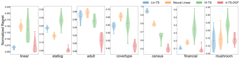
Figure 1: Normalized Cumulative Regret on all settings.

5 Conclusion

In this paper, we proposed a scalable Thompson sampling framework $\pi$-TS for posterior application in Thompson sampling. We approximate the posterior distribution without an explicit-form variational distribution assumption, which leverages more powerful uncertainty estimation ability. Importantly, our methods can be applied on large-scale problems with complex models, such as neural networks. Specifically, $\pi$-TS approximates a distribution by defining gradient flows on the space of probability measures, and uses particles for approximation. Extensive experiments are conducted, demonstrating the effectiveness and efficiency of our proposed $\pi$-TS framework. Interesting future work includes designing more practically efficient variants of $\pi$-TS, and developing theory to study general regret bounds of the algorithms, as was done in [17, 28].

Supplementary Material
Scalable Thompson Sampling via Optimal Transport

Appendix A Details of Experiments

A.1 Brief Dataset Description

The dimensions of actions and contexts of different datasets are shown in Table 1.

Table 1: Description of datasets

Dataset	Contexts	Actions
Mushroom	22	2
Statlog	16	7
Covertype	54	7
Financial	21	8
Census	389	9
Adult	94	14

A.2 More Details of the Results

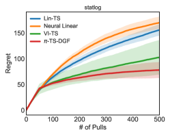
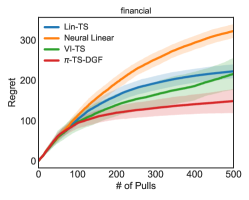
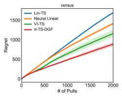
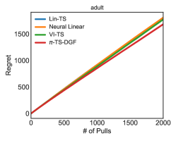
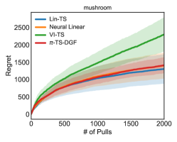
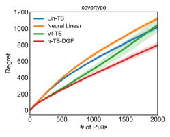
Figure 2: Normalized Regret comparison on real-world datasets.

Table 2: Normalized accumulative regret of all methods.

	Statlog	Adult	Covertype	Census	Financial	Mushroom
Lin-TS	18.62 $\pm$ 0.02	96.71 $\pm$ 0.09	59.32 $\pm$ 0.08	94.54 $\pm$ 0.28	10.48 $\pm$ 0.04	13.22 $\pm$ 0.13
Neural Linear	13.96 $\pm$ 0.03	97.55 $\pm$ 0.06	65.51 $\pm$ 0.07	79.15 $\pm$ 0.32	17.76 $\pm$ 0.06	14.25 $\pm$ 0.12
VI-TS	23.32 $\pm$ 0.09	95.66 $\pm$ 0.08	60.99 $\pm$ 0.25	64.85 $\pm$ 0.91	35.2 $\pm$ 0.31	23.32 $\pm$ 0.16
$\pi$-TS-DGF	5.37 $\pm$ 0.03	90.76 $\pm$ 0.11	46.48 $\pm$ 0.10	49.85 $\pm$ 0.52	8.23 $\pm$ 0.10	14.29 $\pm$ 0.07

A.3 Effects of Numbers of Particles

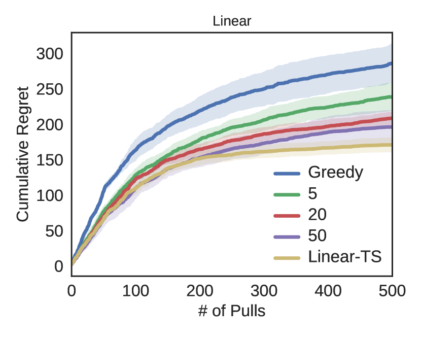
Figure 3: Impact of particle number.

We investigate the influence of different number of particles used on the performance. We choose different number of particles as $M=1,5,20,50$, where the case of 1 particle corresponds to the greedy setting. We use the same model as the above experiments. In this part, we use larger noise $\sigma_{i}^{2}=0.1$, and pull each arm 2 times at the initial stage. Figure 3 shows accumulated regrets along with number of particles. As expected, the best performance is achieved with the largest number of particles. The performance keep improving with increasing particles, but the gain becomes insignificant considering the increased computational costs.

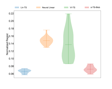
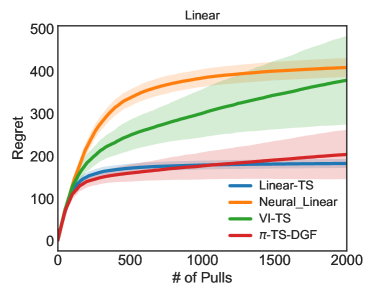
Figure 4: Normalized Regret comparison among four methods on linear cases.

A.4 Linear Rewards

We consider a contextual bandit with $k=8$ arms and $d=10$ dimensional contexts. For a given context $X\sim\mathcal{N}(\mu,\Sigma)$, the reward obtained by pulling arm $i$ follows a linear model $r_{i,X}=X^{T}\beta_{i}+\epsilon$ with $\epsilon\sim\mathcal{N}(0,\sigma_{i}^{2})$, where $\sigma_{i}^{2}=0.01i$ The posterior distribution over $\beta_{i}\in\mathrm{R}^{d}$ can be exactly computed using the standard Bayesian linear regression formula, denoted as Lin-TS. We set the contextual dimension $d=20$, and the prior to be $\beta\sim\mathcal{N}(0,\lambda\ \text{I}_{d})$, for $\lambda>0$. The results in terms of both regret and normalized regret are plotted in Figure 4. We can see from the figure that the proposed methods, $\pi$-TS-Blob and $\pi$-TS-DGF, perform almost as well as Lin-TS, the exact model; whereas other methods such as Neural-Linear and VI-TS receive much larger regrets. The gap is mostly caused by the approximation error between the exact posterior and approximate posterior. Especially, VI-TS shows a higher regret variance. Furthermore, both $\pi$-TS-Blob and $\pi$-TS-DGF are found performed similarly.

A.5 Sparse Linear Rewards

In this case, the weight vector $\beta^{s}_{i}\in\mathrm{R}^{d}$ is sparse. Specifically, $\beta^{s}_{i}$ is more sparse than the standard $\beta$ used above. The reward obtained by pulling arm $i$ follows a sparse linear model is $r_{i,X}=X^{T}\beta^{s}_{i}+\epsilon$, where $\sigma_{i}^{2}=0.01i$. The results are plotted in Figure 5. Similarly, much less regrets are achieved by $\pi$-TS-DGF, which is comparable to Lin-TS.

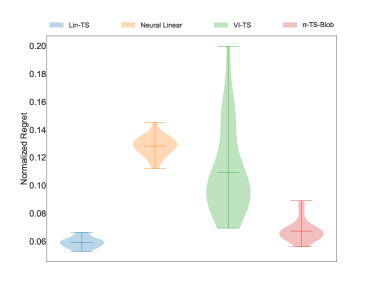
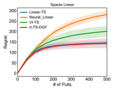
Figure 5: Normalized Regret comparison among five methods on sparse linear cases.

Appendix B More Details of Methods

B.1 Vanilla Thompson Sampling

Algorithm 2 Thompson Sampling (Vanilla Version)

0:  prior distribution $p_{0}$

1:  for $t=1,2,\ldots,T$ do

2:     Observe context $\operatorname{\mathbf{x}}_{t}$

3:     Draw $\hat{{\bm{\mathchar 28946\relax}}}_{t}$ from the posterior $p_{t-1}$

4:     Select $\operatorname{\mathbf{a}}_{t}\in\arg\max_{\operatorname{\mathbf{a}}}m(\operatorname{\mathbf{x}}_{t},\operatorname{\mathbf{a}};\hat{{\bm{\mathchar 28946\relax}}}_{t})$

5:     Observe and receive reward $r_{t}$

6:     Update posterior $p_{t}({\bm{\mathchar 28946\relax}})\leftarrow p_{t-1}({\bm{\mathchar 28946\relax}}|(\operatorname{\mathbf{x}}_{t},\operatorname{\mathbf{a}}_{t},r_{t}))$.

7:  end for

B.2 Gradient Flows in Euclidean space

For ease of understanding, we first motivate from gradient flows on the Euclidean space in the following. For a smooth function $F:\mathbb{R}^{d}\rightarrow\mathbb{R}$, and a starting point ${\bm{\mathchar 28946\relax}}_{0}\in\mathbb{R}^{d}$, the gradient flow of $F({\bm{\mathchar 28946\relax}})$ is defined as the solution of the differential equation: $\frac{\mathrm{d}{\bm{\mathchar 28946\relax}}}{\mathrm{d}\tau}=-\nabla F({\bm{\mathchar 28946\relax}}(\tau))$, for time $\tau>0$ and initial condition ${\bm{\mathchar 28946\relax}}(0)={\bm{\mathchar 28946\relax}}_{0}$. This is a standard Cauchy problem [20], endowed with a unique solution if $\nabla F$ is Lipschitz continuous. When $F$ is non-differentiable, the gradient is replaced with its subgradient, which gives a similar definition, omitted here for simplicity.

We consider a contextual bandit with $k=8$ arms and $d=10$ dimensional contexts. For a given context $X\sim\mathcal{N}(\mu,\Sigma)$, the reward obtained by pulling arm $i$ follows a linear model $r_{i,X}=X^{T}\beta_{i}+\epsilon$ with $\epsilon\sim\mathcal{N}(0,\sigma_{i}^{2})$, where $\sigma_{i}^{2}=0.01i$ The posterior distribution over $\beta_{i}\in\mathrm{R}^{d}$ can be exactly computed using the standard Bayesian linear regression formula, denoted as Lin-TS. We set the contextual dimension $d=20$, and the prior to be $\beta\sim\mathcal{N}(0,\lambda\ \text{I}_{d})$, for $\lambda>0$.

Appendix C Related Work

It is difficult in general to calculate exact posteriors in Thompson sampling. Thus it is necessary to efficiently approximate a posterior distribution to make TS scalable for complex models. [7] first used standard variational inference to approximate the posterior of neural networks, i.e., Bayesian neural networks, which were then incorporated into Thompson sampling. Further, [18] proposed to use different heads for a deep Q-network to approximate posterior with bootstrap. Inspired by [18], [17] proposed ensemble sampling, which uses a set of particles to approximate a posterior distribution. These particles are updated independently with stochastic gradient descent, without a convergence guarantee, in terms of posterior-approximation convergence. Similarly, weighted bootstrap [26] uses random weights performed on the likelihood to mimic the bootstrap, which is connected to TS. [19] built a benchmark to evaluate deep Bayesian bandits, and especially recommended the neural linear method, which uses a deep neural network to extract features and perform linear Thompson sampling based on these features. Similar to neural linear, [6] replaced the final layer of a deep neural network with Bayesian logistic regression for deep Q-networks, which greatly boosted the performance on Atari benchmarks. [30] firstly investigate particle-based Thompson sampling in contextual bandits settings. [29] places policy optimization into the space of probability measures, and interpret it as Wasserstein gradient flows. In this work, we provide a distribution optimization perspective to understand the posterior approximation, and propose efficient algorithms to approximate posterior distributions in Thompson sampling. This work can be regarded as the counterpart of [30] for value-based methods.

References

- [1] Rajeev Agrawal. Sample mean based index policies by o (log n) regret for the multi-armed bandit problem. Advances in Applied Probability, 1995.
- [2] Shipra Agrawal and Navin Goyal. Analysis of thompson sampling for the multi-armed bandit problem. In COLT, 2012.
- [3] Shipra Agrawal and Navin Goyal. Thompson sampling for contextual bandits with linear payoffs. In ICML, 2013.
- [4] L. Ambrosio, N. Gigli, and G. Savaré. Gradient Flows in Metric Spaces and in the Space of Probability Measures. Lectures in Mathematics ETH Zürich, 2005.
- [5] Peter Auer. Using confidence bounds for exploitation-exploration trade-offs. JMLR, 2002.
- [6] Kamyar Azizzadenesheli, Emma Brunskill, and Animashree Anandkumar. Efficient exploration through bayesian deep q-networks. arXiv:1802.04412, 2018.
- [7] Charles Blundell, Julien Cornebise, Koray Kavukcuoglu, and Daan Wierstra. Weight uncertainty in neural networks. In ICML, 2015.
- [8] Sébastien Bubeck, Nicolo Cesa-Bianchi, et al. Regret analysis of stochastic and nonstochastic multi-armed bandit problems. Foundations and Trends® in Machine Learning, 2012.
- [9] Manfredo Perdigão do Carmo. Riemannian geometry. Birkhäuser, 1992.
- [10] Nicolò Cesa-Bianchi, Claudio Gentile, Gábor Lugosi, and Gergely Neu. Boltzmann exploration done right. In NIPS, 2017.
- [11] Olivier Chapelle and Lihong Li. An empirical evaluation of thompson sampling. In NIPS, 2011.
- [12] Changyou Chen, Ruiyi Zhang, Wenlin Wang, Bai Li, and Liqun Chen. A unified particle-optimization framework for scalable bayesian sampling. In UAI, 2018.
- [13] Günay Dogan and Ricardo H Nochetto. First variation of the general curvature-dependent surface energy. ESAIM: Mathematical Modelling and Numerical Analysis.
- [14] Richard Jordan, David Kinderlehrer, and Felix Otto. The variational formulation of the fokker–planck equation. SIMA, 1998.
- [15] Lihong Li, Wei Chu, John Langford, and Robert E Schapire. A contextual-bandit approach to personalized news article recommendation. In WWW, 2010.
- [16] Qiang Liu and Dilin Wang. Stein variational gradient descent: A general purpose bayesian inference algorithm. In NIPS, 2016.
- [17] Xiuyuan Lu and Benjamin Van Roy. Ensemble sampling. In NIPS, 2017.
- [18] Ian Osband, Charles Blundell, Alexander Pritzel, and Benjamin Van Roy. Deep exploration via bootstrapped dqn. In NIPS, 2016.
- [19] Carlos Riquelme, George Tucker, and Jasper Snoek. Deep bayesian bandits showdown: An empirical comparison of bayesian deep networks for thompson sampling. In ICLR, 2018.
- [20] Jim Rulla. Error analysis for implicit approximations to solutions to cauchy problems. SINUM, 1996.
- [21] Daniel Russo and Benjamin Van Roy. An information-theoretic analysis of thompson sampling. JMLR, 2016.
- [22] Daniel J Russo, Benjamin Van Roy, Abbas Kazerouni, Ian Osband, Zheng Wen, et al. A tutorial on thompson sampling. Foundations and Trends® in Machine Learning, 2018.
- [23] Richard S Sutton. Integrated architectures for learning, planning, and reacting based on approximating dynamic programming. In Machine Learning Proceedings. Elsevier, 1990.
- [24] Richard S Sutton and Andrew G Barto. Introduction to reinforcement learning. MIT press Cambridge, 1998.
- [25] William R Thompson. On the likelihood that one unknown probability exceeds another in view of the evidence of two samples. Biometrika, 1933.
- [26] Sharan Vaswani, Branislav Kveton, Zheng Wen, Anup Rao, Mark Schmidt, and Yasin Abbasi-Yadkori. New insights into bootstrapping for bandits. arXiv:1805.09793, 2018.
- [27] C. Villani. Optimal transport: old and new. Springer Science & Business Media, 2008.
- [28] Jianyi Zhang, Ruiyi Zhang, and Changyou Chen. Stochastic particle-optimization sampling and the non-asymptotic convergence theory. arXiv:1809.01293, 2018.
- [29] Ruiyi Zhang, Changyou Chen, Chunyuan Li, and Lawrence Carin. Policy optimization as wasserstein gradient flows. In ICML, 2018.
- [30] Ruiyi Zhang, Chunyuan Li, Changyou Chen, and Lawrence Carin. Learning structural weight uncertainty for sequential decision-making. In AISTATS, 2018.