Learning Optimal Linear Regularizers

Abstract

We present algorithms for efficiently learning regularizers that improve generalization. Our approach is based on the insight that regularizers can be viewed as upper bounds on the generalization gap, and that reducing the slack in the bound can improve performance on test data. For a broad class of regularizers, the hyperparameters that give the best upper bound can be computed using linear programming. Under certain Bayesian assumptions, solving the LP lets us “jump” to the optimal hyperparameters given very limited data. This suggests a natural algorithm for tuning regularization hyperparameters, which we show to be effective on both real and synthetic data.

1 Introduction

Most machine learning models are obtained by minimizing a loss function, but optimizing the training loss is rarely the ultimate goal. Instead, the model is ultimately judged based on information that is unavailable during training, such as performance on held-out test data. The ultimate value of a model therefore depends critically on the loss function one chooses to minimize.

Traditional loss functions used in statistical learning are the sum of two terms: the empirical training loss and a regularization penalty. A common regularization penalty is the $\ell^{1}$ or $\ell^{2}$ norm of the model parameters. More recently, it has become common to regularize implicitly by perturbing the examples, as in dropout (Srivastava et al., 2014), or perturbing the labels, as in label smoothing (Szegedy et al., 2016), or by modifying the training algorithm, as in early stopping (Caruana et al., 2001).

The best choice of regularizer is usually not obvious a priori. Typically one chooses a regularizer that has worked well on similar problems, and then fine-tunes it by searching for the hyperparameter values that give the best performance on a held-out validation set. Though this approach can be effective, it tends to require a large number of training runs, and to mitigate this the number of hyperparameters must be kept fairly small in practice.

In this work, we seek to recast the problem of choosing regularization hyperparameters as a supervised learning problem which can be solved more efficiently than is possible with a purely black-box approach. Specifically, we show that the optimal regularizer is by definition the one that provides the tightest possible bound on the generalization gap (i.e., difference between test and training loss), for a suitable notion of “tightness”. We then present an algorithm that can find approximately optimal regularization hyperparameters efficiently via linear programming. Our method applies to explicit regularizers such as L2, but also in an approximate way to implicit regularizers such as dropout.

Our algorithm takes as input a small set of models for which we have computed both training and validation loss, and produces a set of recommended regularization hyperparameters as output. Under certain Bayesian assumptions, we show that our algorithm returns the optimal regularization hyperparameters, requiring data from as few as two training runs as input. Building on this linear programming algorithm, we present a hyperparameter tuning algorithm and show that it outperforms state-of-the-art alternatives on real problems where these assumptions do not hold.

1.1 Definitions and Notation

We consider a general learning problem with an arbitrary loss function. Our goal is to choose a hypothesis $\theta\in\Theta$, so as to minimize the expected value of a loss function $\ell(z,\theta)$ for an example $z$ drawn from an unknown distribution $\mathcal{D}$. That is, we wish to minimize

$$L(\theta)=\mathbb{E}_{z\sim\mathcal{D}}[\ell(z,\theta)]\mbox{ .}$$

In a typical supervised learning problem, $\theta$ is a parameter vector, $z$ is a (feature vector, label) pair, and $\ell$ is a loss function such as log loss or squared error. In an unsupervised problem, $z$ might be an unlabeled image or a text fragment.

We assume as input a set $\left\{z_{i}\ |\ 1\leq i\leq n\right\}$ of training examples. Where noted, we assume each $z_{i}$ is sampled independently from $\mathcal{D}$. We denote average training loss by:

$$\hat{L}(\theta)=\frac{1}{n}\sum_{i=1}^{n}\ell(z_{i},\theta)\mbox{ .}$$

We will focus on algorithms that minimize an objective function $f(\theta)=\hat{L}(\theta)+R(\theta)$, where $R:\Theta\rightarrow\mathbb{R}_{>0}$ is the regularizer (the choice of which may depend on the training examples). We denote the minimizer of regularized loss by

$$\hat{\theta}=\operatorname*{argmin}_{\theta\in\Theta}\left\{\hat{L}(\theta)+R(\theta)\right\}$$

and the optimal hypothesis by

$$\theta^{*}=\operatorname*{argmin}_{\theta\in\Theta}\left\{L(\theta)\right\}\mbox{ .}$$

We refer to the gap $L(\hat{\theta})-L(\theta^{*})$ as excess test loss. Our goal is to choose $R$ so that the excess test loss is as small as possible.

2 Regularizers and Generalization Bounds

Our strategy for learning regularizers will be to compute a regularizer that provides the tightest possible estimate of the generalization gap (difference between test and training loss). To explain the approach, we begin with a mathematically trivial yet surprisingly useful observation:

$$R(\theta)=L(\theta)-\hat{L}(\theta)\implies L(\hat{\theta})=L(\theta^{*})\mbox{ .}$$

That is, the generalization gap is by definition an optimal regularizer, since training with this regularizer amounts to training directly on the test loss. More generally, for any monotone function $h$, the regularizer $R(\theta)=h(L(\theta))-\hat{L}(\theta)$ is optimal.

Though training directly on the test loss is clearly not a workable strategy, we might hope to use a regularizer that accurately estimates the generalization gap, so that regularized training loss estimates test loss. What makes a good estimate in this context?

In supervised learning we typically seek an estimate with good average-case performance, for example low mean squared error. However, that fact that $\hat{\theta}$ is obtained by optimizing over all $\theta\in\Theta$ means that a single bad estimate could make $L(\hat{\theta})$ arbitrarily bad, suggesting that worst-case error matters. At the same time, it should be less important to estimate $L(\theta)$ accurately if $\theta$ is far from optimal. The correct characterization turns out to be:

A good regularizer is one that provides an upper bound on the generalization gap that is tight at near-optimal points.

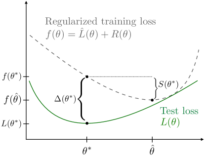
Figure 1: Suboptimality ($S$) and slack ($\Delta$).

To formalize this, we introduce two quantities. For a fixed regularizer $R$, defining a regularized training loss $f(\theta)=\hat{L}(\theta)+R(\theta)$, define the slack of $R$ at a point $\theta$ as

$$\Delta(\theta)\equiv f(\theta)-L(\theta)\mbox{ .}$$

For any $\theta$, define the suboptimality as $S(\theta)\equiv f(\theta)-f(\hat{\theta})$. Figure 1 illustrates these definitions.

We now give an expression for excess test loss in terms of slack and suboptimality. For any $\theta$, $L(\theta)=f(\theta)-\Delta(\theta)$, so

$$L(\hat{\theta})-L(\theta) =f(\hat{\theta})-\Delta(\hat{\theta})-f(\theta)+\Delta(\theta)$$

$$=\Delta(\theta)-\Delta(\hat{\theta})-S(\theta)$$

$$\equiv\mathsf{SAS}(\theta)\mbox{ .}$$

We refer to the quantity $\mathsf{SAS}(\theta)$ as suboptimality-adjusted slack. Maximizing both sides over all $\theta\in\Theta$ gives an expression for excess test loss:

$$L(\hat{\theta})-L(\theta^{*})=\max_{\theta\in\Theta}\left\{\mathsf{SAS}(\theta)\right\}\mbox{ .}$$

That is, the excess test loss of a hypothesis $\hat{\theta}$ obtained by minimizing $\hat{L}(\theta)+R(\theta)$ is the worst-case suboptimality-adjusted slack. An optimal regularizer is therefore one that minimizes this quantity. This is summarized in the following proposition.

Proposition 1.

For any set $\Theta$ of hypotheses, and any set $\mathcal{R}$ of regularizers, the optimal regularizer is

$$\operatorname*{argmin}_{R\in\mathcal{R}}\left\{L(\hat{\theta}(R))\right\}=\operatorname*{argmin}_{R\in\mathcal{R}}\left\{\max_{\theta\in\Theta}\left\{\mathsf{SAS}(\theta;R)\right\}\right\}$$

where $\hat{\theta}$ and $\mathsf{SAS}$ are defined as above, with the dependence on $R$ now made explicit.

How can we make use of Proposition 1 in practice? We do not of course know the test loss for all $\theta\in\Theta$, and thus we cannot compute $\max_{\theta\in\Theta}\left\{\mathsf{SAS}(\theta;R)\right\}$ exactly. However, it is feasible to compute the validation loss for a small set $\Theta_{0}\subseteq\Theta$ of hypotheses, for example by doing multiple training runs with different regularization hyperparameters, or doing a single run with different thresholds for early stopping. We can then compute an approximately optimal regularizer using the approximation:

$$R^{*}\approx\operatorname*{argmin}_{R\in\mathcal{R}}\left\{\max_{\theta\in\Theta_{0}}\left\{\hat{\mathsf{SAS}}(\theta;R)\right\}\right\}$$ (1)

where $\hat{\mathsf{SAS}}$ is an estimate of $\mathsf{SAS}$ that uses validation loss as a proxy for test loss, and uses $\Theta_{0}$ as a proxy for $\Theta$.

Importantly, the $R^{*}$ given by equation 1 will generally not be one of the regularizers we already tried when producing the models in $\Theta_{0}$, as is shown formally in Theorem 1.

This suggests a simple iterative procedure for tuning regularization hyperparameters. Initially, let $\Theta_{0}$ be a small set of hypotheses trained using a few different hyperparameter settings. Then, use approximation (1) to compute an approximately optimal regularizer $R_{1}$ based on $\Theta_{0}$. Then, train a hypothesis $\theta_{1}$ using $R_{1}$, and add it to $\Theta_{0}$ to obtain a new set $\Theta_{1}=\Theta_{0}\cup\left\{\theta_{1}\right\}$, use $\Theta_{1}$ to obtain a better approximation $R_{2}$, and so on.

2.1 Implicit Regularizers

So far we have assumed the regularizer is an explicit function of the model parameters, but many regularizers used in deep learning do not take this form. Instead, they operate implicitly by perturbing the weights, labels, or examples. Is Proposition 1 still useful in this case?

It turns out to be straightforward to accomodate such regularizers. To illustrate, let $P(\theta)$ be a (possibly randomized) perturbation applied to $\theta$. Training with the loss function $\mathbb{E}[\hat{L}(P(\theta))]$ is equivalent to using the regularizer

$$R(\theta)=\mathbb{E}[\hat{L}(P(\theta))]-\hat{L}(\theta)\mbox{ .}$$

In the case of dropout, $P(\theta)$ sets each activation in a layer to 0 independently with some probability $p$, which is equivalent to setting the corresponding outgoing weights to zero. The regularizer is simply the expected difference between training loss using the perturbed weights and training loss using the original weights. This observation, together with Proposition 1, yields the following conclusion:

The best dropout probability is the one that makes the gap between training loss with and without dropout be the tightest possible estimate of the generalization gap (where tightness is worst-case suboptimality-adjusted slack).

Similar constructions can be used to accomodate implicit regularizers that perturb the labels (as in label smoothing) or the input data (as in data augmentation). More generally, we can view any perturbation as a potentially useful regularizer. For example, training with quantized model weights can be viewed as using a regularizer equal to the increase in training loss that quantization introduces. Quantization will be effective as a regularizer to the extent that this increase provides a tight estimate of the generalization gap.

3 Learning Linear Regularizers

We now consider the problem of computing an approximately optimal regularizer from some set $\mathcal{R}$ of possible regularizers, given as input a set $\Theta_{0}$ of hypotheses for which we have computed both training and validation loss. In practice, the models in $\Theta_{0}$ might be the result of training for different amounts of time, or using different hyperparameters.

We will present an algortihm for computing the best linear regularizer, defined as follows.

Definition 1.

A linear regularizer is a function of the form

$$R(\theta;\lambda)=\lambda\cdot q(\theta)$$

where $q:\Theta\rightarrow\mathbb{R}^{k}$ is a function that, given a model, returns a feature vector of length $k$.

Commonly-used regularizers such as L1 and L2 can be expressed as linear regularizers by including the L1 or L2 norm of the model in the feature vector, and novel regularizers can be easily defined by including additional features. We consider the case where $\mathcal{R}=\left\{R(\cdot;\lambda):\lambda\in\mathbb{R}^{k}\right\}$ is the set of all linear regularizers using a fixed feature vector $q(\theta)$.

Dropout is not a linear regularizer, because the implicit regularization penalty, $R(\theta,p)=\mathbb{E}[\hat{L}(\mathrm{dropout}(\theta,p))]-\hat{L}(\theta)$, varies nonlinearly as a function of the dropout probability $p$. However, dropout can be approximated by a linear regularizer using a feature vector of the form $q(\theta)=\langle R(\theta,p_{1}),R(\theta,p_{2}),\ldots,R(\theta,p_{k})\rangle$, for a suitably fine grid of dropout probabilties $\left\{p_{1},p_{2},\ldots,p_{k}\right\}$.

Our algorithm for computing the best linear regularizer is designed to have two desirable properties:

1. Consistency: in the limiting case where $\Theta_{0}=\Theta$, and validation loss is an exact estimate of test loss, it recovers an optimal regularizer.

2. Efficiency: in the case where there exists a regularizer that perfectly estimates the generalization gap, we require only $k+1$ data points in order to recover it.

To describe our algorithm, let $V(\theta)$ be average loss on a validation set. To guarantee consistency, it is sufficient that we return the regularizer $R\in\mathcal{R}$ that minimizes the validation loss of $\hat{\theta}_{0}(R)$, where $\hat{\theta}_{0}(R)$ is the model in $\Theta_{0}$ that minimizes regularized training loss when $R$ is the regularizer. That is, we wish to find the regularizer

$$\hat{R}\equiv\operatorname*{argmin}_{R\in\mathcal{R}}\left\{V(\hat{\theta}_{0}(R))\right\}$$

where $\hat{\theta}_{0}(R)\equiv\operatorname*{argmin}_{\theta\in\Theta_{0}}\left\{\hat{L}(\theta)+R(\theta)\right\}$.

This regularizer can be computed as follows. For each $\theta_{i}\in\Theta_{0}$, we solve a linear program to compute a function of the form $f(\theta)=\hat{L}(\theta)+\lambda\cdot q(\theta)$, subject to the constraint that $\theta_{i}=\operatorname*{argmin}_{\theta\in\Theta_{0}}\left\{f(\theta)\right\}$, or equivalently $f(\theta_{i})\leq f(\theta)\ \forall\theta\in\Theta_{0}$. Among the $\theta_{i}$’s for which the LP is feasible, the one with minimum $V(\theta_{i})$ determines $\hat{R}$. Knowing this, we consider the $\theta_{i}$’s in ascending order of $V(\theta_{i})$, stopping as soon as we find an LP that is feasible.

To guarantee efficiency, we must include additional constraints in our linear program that break ties in the case where there are multiple values of $\lambda$ that produce the same argmin of $f$. As we will show in Theorem 1, a sufficient constraint is that $f$ is an upper bound on validation loss that minimizes total slack. Additionally, our linear program gives us the freedom to upper bound $\alpha V(\theta)$ rather than $V(\theta)$ (for some $\alpha>0$), which is necessary for the guarantees proved in §4. Pseudocode is given below.

  Input: Set of (validation loss, training loss, feature vector) tuples $\left\{(V_{i},\hat{L}_{i},q_{i})\ |\ 1\leq i\leq m\right\}$.

  Sort tuples in ascending order of $V_{i}$, and reindex so that $V_{1}\leq V_{2}\leq\ldots\leq V_{m}$.

  for $i^{*}$ from $1$ to $m$ do

     Solve the following linear program:

$$\begin{array}[]{lll}\text{minimize}&\sum_{i=1}^{m}\Delta_{i}&\\ \text{subject to}&\alpha\geq 0\\ &\Delta_{i}\geq 0&\forall i\\ &f_{i}=\alpha V_{i}+\Delta_{i}&\forall i\\ &f_{i}=\lambda\cdot q_{i}+\hat{L}_{i}&\forall i\\ &f_{i^{*}}\leq f_{i}&\forall i\\ \end{array}$$

     If the LP is feasible, return $(\alpha,\lambda)$.

  Return error.

Algorithm LearnLinReg

By construction, LearnLinReg returns the linear regularizer that would have given the best possible validation loss, when minimizing regularized training loss over all $\theta\in\Theta_{0}$. This guarantees consistency, as summarized in Proposition 2.

Proposition 2.

Assuming it terminates successfully, LearnLinReg returns a pair $(\alpha^{*},\lambda^{*})$ such that

$$R(\cdot;\lambda^{*})=\operatorname*{argmin}_{R\in\mathcal{R}}\left\{V(\hat{\theta}_{0}(R))\right\}\mbox{ .}$$

We now consider efficiency. In the case where there exists a $\lambda^{*}$ that allows for perfect estimation of validation loss, Theorem 1 shows that LearnLinReg can recover $\lambda^{*}$ provided $\Theta_{0}$ contains as few as $k+1$ hypotheses, where $k$ is the size of the feature vector.

Theorem 1.

Suppose there exists a perfect regularizer, in the sense that for some vector $\lambda^{*}$ and scalar $\alpha^{*}>0$,

$$\alpha^{*}V(\theta)=\hat{L}(\theta)+\lambda^{*}\cdot q(\theta)\quad\quad\forall\theta\in\Theta\mbox{ .}$$

Let $D=\left\{(V(\theta_{i}),\hat{L}(\theta_{i}),q(\theta_{i}))\ |\ 1\leq i\leq k+1\right\}$ be a set of tuples such that the vectors $\langle V(\theta_{i}),\hat{L}(\theta_{i})\rangle\oplus q(\theta_{i})$ are linearly independent, where $k=|q(\theta)|$. Then, $LearnLinReg(D)$ will return $(\alpha^{*},\lambda^{*})$.

Proof.

Under these assumptions, the first LP considered by LearnLinReg has a feasible point $\alpha=\alpha^{*}$, $\lambda=\lambda^{*}$, and $\Delta_{i}=0\ \forall i$. Because each $\Delta_{i}$ is constrained to be non-negative, this point must be optimal, and thus any optimal point must have $\Delta_{i}=0\ \forall i$. Thus, any optimal point must satisfy $\alpha V(\theta_{i})=\lambda\cdot q(\theta_{i})+\hat{L}(\theta_{i})\ \forall i$. This is a system of linear equations with $k+1$ variables, and by assumption the equations are linearly independent. Thus the solution is unique, and the algorithm returns $(\alpha^{*},\lambda^{*})$. ∎

If desired, LearnLinReg can be easily modified to only consider $\lambda$ vectors in a feasible set $\mathcal{F}=\prod_{j=1}^{k}[\lambda^{\mathrm{min}}_{j},\lambda^{\mathrm{max}}_{j}]$.

3.1 Hyperparameter Tuning

  Input: training loss $\hat{L}(\theta)$, validation loss $V(\theta)$, feature vector $q(\theta)$, initial set $\Lambda_{0}$ of hyperparameter vectors, training algorithm $\mathrm{train}(\lambda)$, hyperparameter vector sampler $\mathrm{random\_sample}()$.

  Set $\Theta_{0}\leftarrow\left\{\mathrm{train}(\lambda)\ |\ \lambda\in\Lambda_{0}\right\}$, $\Lambda_{\mathrm{seen}}\leftarrow\Lambda_{0}$.

  Set $D\leftarrow\left\{(V(\theta),\hat{L}(\theta),q(\theta))\ |\ \theta\in\Theta_{0}\right\}$.

  while True do

     Set $\_,\lambda\leftarrow\mathrm{LearnLinReg}(D)$.

     If $\lambda\in\Lambda_{\mathrm{seen}}$, set $\lambda\leftarrow\mathrm{random\_sample}()$.

     Set $\theta\leftarrow\mathrm{train}(\lambda)$, and set $\Lambda_{\mathrm{seen}}\leftarrow\Lambda\cup\left\{\lambda\right\}$

     Set $D\leftarrow D\cup\left\{(V(\theta),\hat{L}(\theta),q(\theta))\right\}$.

Algorithm TuneReg

We now describe how to use LearnLinReg for hyperparameter tuning. Given an initial set of hyperparameter vectors, we train using each one, and observe the resulting training and validation loss, as well as the feature vector for the trained model. We then feed this data to LearnLinReg to obtain a vector $\lambda$ of regularization hyperparameters. We then train using these hyperparameters, add the results to our dataset, and re-run LearnLinReg. Experiments using this algorithm are presented in §5.

4 Recovering Bayes-Optimal Regularizers

We have shown that a regularizer is optimal if it can be used to perfectly predict the generalization gap, and have presented an algorithm that can efficiently recover a linear regularizer if a perfect one exists. Do perfect linear regularizers ever exist? Perhaps surprisingly, the answer is “yes” for a broad class of Bayesian inference problems.

As discussed in §1.1, we assume examples are drawn from a distribution $\mathcal{D}$. In the Bayesian setting, we assume that $\mathcal{D}$ itself is drawn from a (known) prior distribution $\mathcal{D}_{1}$. Given a training dataset $Z\sim\mathcal{D}^{n}$, where $\mathcal{D}\sim\mathcal{D}_{1}$, we now care about the conditional expected test loss:

$$\bar{L}(\theta,Z)\equiv E_{\mathcal{D}\sim\mathcal{D}_{1}}[L(\theta,\mathcal{D})|Z]$$

where $L(\theta,\mathcal{D})=\mathbb{E}_{z\sim\mathcal{D}}[\ell(z,\theta)]$ as in §1.1. A Bayes-optimal regularizer is one which minimizes this quantity.

Definition 2.

Given a training set $Z\sim\mathcal{D}^{n}$, where $\mathcal{D}\sim\mathcal{D}_{1}$, a Bayes-optimal regularizer is a regularizer $R^{*}$ that satisfies:

$$\operatorname*{argmin}_{\theta\in\Theta}\left\{\hat{L}(\theta)+R^{*}(\theta)\right\}=\operatorname*{argmin}_{\theta\in\Theta}\left\{\bar{L}(\theta,Z)\right\}\mbox{ .}$$

$R^{*}$ is perfect if, additionally, it satisfies the stronger condition

$$\hat{L}(\theta)+R^{*}(\theta)=h(\bar{L}(\theta,Z))\ \forall\theta\in\Theta$$

for some monotone function $h$.

Theorem 2 shows that a perfect Bayes-optimal regularizer exists for density estimation problems where log loss is the loss function, $\theta$ parameterizes an exponential family distribution $\mathcal{D}$ from which examples are drawn, and $\mathcal{D}_{1}$ is the conjugate prior for $\mathcal{D}$.

Theorem 2.

Let $P(z|\theta)$ be an exponential family distribution with natural parameter $\eta(\theta)$ and conjugate prior $P(\theta)$, and suppose the following hold:

1. $z\sim\mathcal{D}$, where $\mathcal{D}=P(z|\theta^{*})$.

2. $\ell(z,\theta)=-\log P(z|\theta)$.

3. $\theta^{*}\sim P(\theta)$.

Then, for any training set $Z\sim\mathcal{D}^{n}$, $R^{*}$ is a perfect, Bayes-optimal regularizer, where

$$R^{*}(\theta)=-\frac{1}{n}\log P(\eta(\theta))\mbox{ .}$$

The proof is given in Appendix A.

In the special case where $\theta$ is the natural parameter (i.e., $\eta(\theta)=\theta$), Theorem 2 gives $R^{*}(\theta)=-\frac{1}{n}\log P(\theta)$. Using Bayes’ rule, it can be shown that minimizing $\hat{L}(\theta)+R^{*}(\theta)$ is equivalent to maximizing the posterior probability of $\theta$ (i.e., performing MAP inference).

4.1 Example: Coin Flips

Suppose we have a collection of coins, where coin $i$ comes up heads with unknown probability $p_{i}$. Given a training dataset consisting of outcomes from flipping each coin a certain number of times, we would like to produce a vector $\theta$, where $\theta_{i}$ is an estimate of $p_{i}$, so as to minimize expected log loss on test data. This can be viewed as a highly simplified version of the problem of click-through rate prediction for online ads (e.g., see McMahan et al. (2013)).

For each coin, assume $p_{i}\sim\mathrm{Beta}(\alpha,\beta)$ for some unknown constants $\alpha$ and $\beta$. Using the fact that the Bernoulli distribution is a member of the exponential family whose conjugate prior is the Beta distribution, and the fact that overall log loss is the sum of the log loss for each coin, we can prove the following as a corollary of Theorem 2.

Corollary 1.

A Bayes-optimal regularizer for the coin flip problem is given by

$$\mathrm{LogitBeta}(\theta)\equiv-\frac{1}{n}\sum_{i}\alpha\log(\theta_{i})+\beta\log(1-\theta_{i})\mbox{ .}$$

Observe that the LogitBeta regularizer is linear, with feature vector $\langle-\sum_{i}\log(\theta_{i}),-\sum_{i}\log(1-\theta_{i})\rangle$.

Given a large validation dataset with many independent coins, it can be shown that validation loss approaches expected test loss. Thus, in the limit, LearnLinReg is guaranteed to recover the optimal hyperparameters (the unknown $\alpha$ and $\beta$) when using this feature vector.

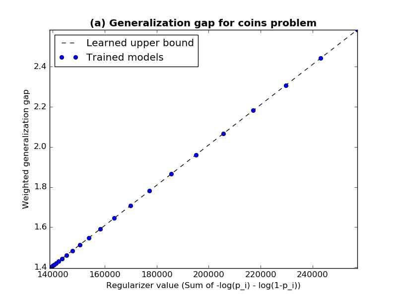
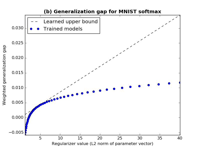
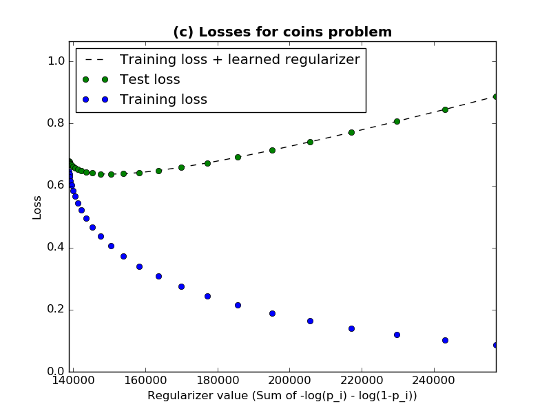
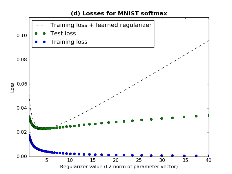
Figure 2: Estimates of the generalization gap for two optimization problems, and corresponding loss functions. For the coins problem, the LogitBeta regularizer perfectly estimates the generalization gap for all models. In contrast, for the MNIST softmax regression problem, L2 regularization provides an upper bound that is only tight for near-optimal models.

Table 1: Comparison of regularizers, in terms of slack (see Figure 1), test loss, and test accuracy.

Problem	Regularizer	Max. slack	Max. adj. slack	Min. test loss	Max. test accuracy
Coins($\lambda^{*}=1$)	LogitBeta	0	0	0.637	–
MNIST Softmax Regression	L1	5.83e-1	1.65e-3	0.0249	99.28%
	L2	1.70	1.95e-4	0.0233	99.31%
	Label smoothing	1.78e-1	2.24e-3	0.0254	99.31%
	Dropout (linearized @ $p=.5$)	6.98e+01	2.92e-2	0.0463	99.34%
Inception-v3 Transfer Learning	L1	1.15	2.36e-2	0.309	90.08%
	L2	1.47	1.11e-4	0.285	90.74%
	Label smoothing	5.03	8.09e-2	0.366	89.65%
	Dropout (linearized @ $p=.5$)	2.52e+1	2.60e-1	0.506	90.46%

5 Experiments

We now evaluate the LearnLinReg and TuneReg algorithms experimentally, using both real and synthetic data. Code for both algorithms is included in the supplementary material.

5.1 Optimization Problems

We consider three optimization problems. The first is an instance of the coin bias estimation problem discussed in §4.1, with $N=10^{5}$ coins whose true bias is drawn from a uniform distribution (a Beta distribution with $\alpha=\beta=1$). Our training data is the outcome of a single flip for each coin, and we compute the test loss $L(\theta)$ exactly.

We then consider two problems that make use of deep networks trained on MNIST and ImageNet (Russakovsky et al., 2015). For MNIST, we train a convolutional neural network using a variant of the LeNet architecture (LeCun et al., 1998). We then consider a softmax regression problem that involves retraining only the last layer of the network. This is a convex optimization problem that we can solve exactly, allowing us to focus on the impact of the regularizer without worrying about the confounding effects of early stopping.

We then consider a transfer learning problem. Starting with an Inception-v3 model trained on ImageNet, we adapt the model to classify images of flowers from a public dataset (The Tensorflow Authors, 2018) split evenly into training and test, retraining the last layer as in (Donahue et al., 2014).

5.2 Comparison of Regularizers

Which regularizers give the tightest generalization bounds? Does tightness in terms of slack translate into good test set performance?

To answer these questions, we solve each of the three optimization problems discussed in §5.1 using a number of different regularizers. For the coins problem, we use the LogitBeta regularizer from Corollary 1, while for the two softmax regression problems we use L1, L2, label smoothing, and a linearized version of dropout. For label smoothing, the loss function is equivalent to $\hat{L}(\theta)+\lambda R(\theta)$, where $R(\theta)$ is average training loss on a set of uniformly-labeled examples. For dropout, the regularizer is the difference between perturbed and unperturbed training loss, with the dropout probability fixed at .5.

For each problem, we proceed as follows. For each regularizer $R_{i}$, and for each $\lambda$ in a predefined grid $\Lambda_{i}$, we generate a model $\hat{\theta}_{i,\lambda}$ by minimizing $\hat{L}(\theta)+\lambda R_{i}(\theta)$. For the coins problem, the solution can be found in closed form, while for the softmax regression problems, we obtain a near-optimal solution by running AdaGrad for 100 epochs. Each grid $\Lambda_{i}$ contains 50 points. For L1 and L2, the grid is log-uniformly spaced over $[.1,100]$, while for label smoothing and dropout it is uniform over $[0,1]$. The result is a set of models, $\Theta_{i}\equiv\left\{\hat{\theta}_{i,\lambda}\ |\ \lambda\in\Lambda_{i}\right\}$.

For each regularizer $R_{i}$, and each $\theta\in\Theta_{i}$, we compute the training loss $\hat{L}(\theta)$, validation loss $V(\theta)$, and regularizer value $R_{i}(\theta)$. We then use LearnLinReg to compute an upper bound on validation loss, using $q_{i}(\theta)\equiv\langle R_{i}(\theta)\rangle$ as the feature vector. This produces a function of the form $f_{i}(\theta)=\hat{L}(\theta)+\lambda^{*}_{i}R_{i}(\theta)$ such that $f_{i}(\theta)\geq\alpha_{i}V(\theta)\ \forall\theta\in\Theta_{i}$.

Figure 2 shows the learned upper bounds for two combinations of problem and regularizer. In all graphs, the horizontal axis is the regularizer value $R_{i}(\theta)$. The top two graphs compare the weighted generalization gap, $\alpha_{i}V(\theta)-\hat{L}(\theta)$, to the learned upper bound $f_{i}(\theta)-\hat{L}(\theta)=\lambda^{*}_{i}R_{i}(\theta)$. For the coins problem (Figure 2 (a)), the learned upper bound is tight for all models, and perfectly predicts the generalization gap. In contrast, for the MNIST softmax regression problem with L2 regularization (Figure 2 (b)), the learned upper bound is only tight at near-optimal models.

Figure 2 (c) and (d) show the corresponding validation loss and (regularized) training loss. In both cases, the argmin of validation loss is very close to the argmin of regularized training loss when using the learned regularization strength, $\lambda^{*}_{i}$. We see qualitatively similar behavior for the other regularizers on both softmax regression problems.

Table 1 compares the upper bounds provided by each regularizers in terms of maximum slack and suboptimality-adjusted slack. To make the numbers comparable, the maximum is taken over all trained models (i.e., all $\theta\in\bigcup_{i}\Theta_{i}$). We also show the minimum test loss and maximum accuracy achieved using each regularizer. Observe that:

• Except for the coins problem, none of the regularizers produces a upper bound whose maximum slack is low (relative to test loss). However, L2 regularization achieves uniformly low suboptimality-adjusted slack.

• The rank ordering of the regularizers in terms of minimum test loss always matches the ordering in terms of maximum suboptimality-adjusted slack.

• Dropout achieves high accuracy despite poor slack and log loss, suggesting its role is somewhat different than that of the more traditional L1 and L2 regularizers.

5.3 Tuning Regularization Hyperparameters

The best values for hyperparameters are typically found empirically using black-box optimization. For regularization hyperparameters, TuneReg provides a potentially more efficient way to tune these hyperparameters, being guaranteed to “jump” to the optimal hyperparameter vector in just $k+1$ steps (where $k$ is the number of hyperparameters) in the special case where a perfect regularizer exists. Does this theoretical guarantee translate into better performance on real-world hyperparameter tuning problems?

To answer this question, we compare TuneReg to random search and to Bayesian optimization using GP-EI-MCMC (Snoek et al., 2012), on each of the three optimization problems. For the coins problem, we use the known optimal LogitBeta regularizer, while for the two softmax regression problems we find a linear combination of the regularizers shown in Table 1 (L1, L2, label smoothing, and linearized dropout). For each problem, TuneReg samples the first $k+1$ points randomly, where $k$ is the number of hyperparameters.

We consider two variants of each algorithm. In both cases, random search and TuneReg sample hyperparameter vectors uniformly from a hypercube, and GP-EI-MCMC uses this hypercube as its feasible set. In the first variant, the hypercube is based on the full range of hyperparameter values considered in the previous section. The second is a more “informed” variant based on data collected when generating Table 1: the feasible range for label smoothing (where applicable) is restricted to $[0,.1]$, and log scaling is applied to the L1, L2, and LogitBeta regularization hyperparameters. Using log scaling is equivalent to sampling from a log-uniform distribution for random search and TuneReg, and to tuning the log of the hyperparameter value for GP-EI-MCMC.

Figure 3 shows the best validation loss achieved by each algorithm as a function of the number of models trained. Each curve is an average of 100 runs. In all cases, TuneReg jumps to near-optimal hyperparameters on step $k+2$, whether or not the initial $k+1$ random points are sampled from the informative distribution ($k=1$ in plot (a), and $k=4$ in plots (b) and (c)). Both variants of TuneReg converge much faster than the competing algorithms, which typically require at least an order of magnitude more training runs in order to reach the same accuracy. The results for TuneReg can be very slightly improved by modifying the LP to enforce that all hyperparameters lie in the feasible range.

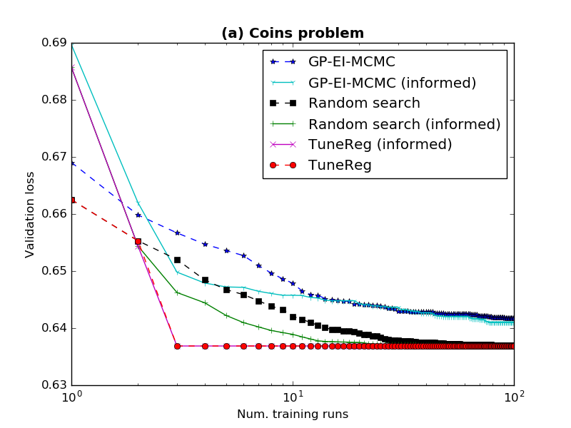
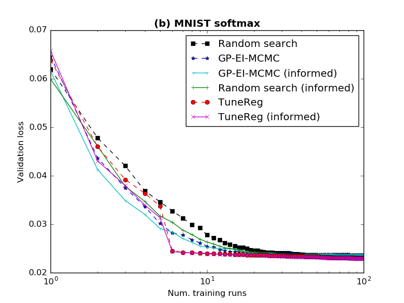
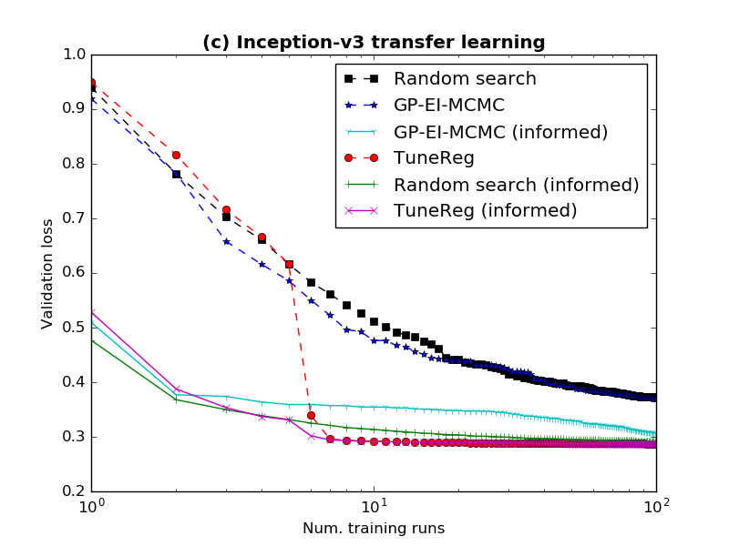
Figure 3: Comparison of algorithms for tuning regularization hyperparameters, with and without informative hyperparameter scaling and feasible range. For problems with $k$ hyperparameters, TuneReg is able to “jump” to near-optimal hyperparameters after randomly sampling $k+1$ initial hyperparameter vectors ($k=1$ in plot (a), $k=4$ in plots (b) and (c)).

6 Related Work

The high-level idea that a good regularizer should provide an estimate of the generalization gap appears to be commonly known, though we are not aware of a specific source. What is novel in our work is the quantitative characterization of good regularizers in terms of slack and suboptimality, and the corresponding linear-programming-based algorithm for finding an approximately optimal regularizer.

Bounding the generalization gap is the subject of a vast literature, which has focused primarily on worst-case bounds (see Zhang et al. (2017) and references therein). These bounds have the advantage of holding with high probability for all models, but are typically too weak to be used effectively as regularizers. In contrast, our empirical upper bounds are only guaranteed to hold for the models we have seen, but are tight enough to yield improved generalization. Empirically, Jiang et al. (2019) showed that the generalization gap can be accurately predicted using a linear model based on margin information; whether this can be used for better regularization is an interesting open question.

An alternative to TuneReg is to use gradient-based methods which (approximately) differentiate validation loss with respect to the regularization hyperparameters (Pedregosa, 2016). Though this idea appears promising, current methods have not been shown to be effective on problems with more than one hyperparameter, and have not produced improvements as dramatic as the ones shown in Figure 3.

7 Conclusions

We have shown that the best regularizer is the one that gives the tightest bound on the generalization gap, where tightness is measured in terms of suboptimality-adjusted slack. We then presented the LearnLinReg algorithm, which computes approximately optimal hyperparameters for a linear regularizer using linear programming. Under certain Bayesian assumptions, we showed that LearnLinReg recovers an optimal regularizer given data from only $k+1$ training runs, where $k$ is the number of hyperparameters. Building on this, we presented the TuneReg algorithm for tuning regularization hyperparameters, and showed that it outperforms state-of-the-art alternatives on both real and synthetic data.

Our experiments have only scratched the surface of what is possible using our high level approach. Promising areas of future work include (a) attempting to discover novel regularizers, for example by making a larger number of basis features available to the LearnLinReg algorithm, and (b) adjusting regularization hyperparameters on-the-fly during training, for example using an online variant of TuneReg.

Appendix A: Additional Proofs

To prove Theorem 2 we will use the following lemma.

Lemma 1.

Suppose that for some functions $q$ and $\phi$, the loss function is of the form:

$$\ell(z,\theta)=q(\theta)\cdot\phi(z)\mbox{ .}$$

Furthermore, suppose there exist constants $n_{0}$ and $\phi_{0}$ such that, for any training set $Z=\left\{z_{i}\ |\ 1\leq i\leq n\right\}$, where $Z\sim\mathcal{D}^{n}$ and $\mathcal{D}\sim\mathcal{D}_{1}$,

$$\mathbb{E}_{\mathcal{D}\sim\mathcal{D}_{1}}[\mathbb{E}_{z\sim\mathcal{D}}[\phi(z)]\ |\ Z]=\frac{\phi_{0}+\sum_{i=1}^{n}\phi(z_{i})}{n+n_{0}}\mbox{ .}$$

Then, there exists a perfect, Bayes-optimal regularizer of the form:

$$R^{*}(\theta)=\frac{1}{n}q(\theta)\cdot\phi_{0}\mbox{ .}$$

Proof.

Let $\bar{L}(\theta,Z)\equiv\mathbb{E}_{D\sim\mathcal{D}_{1}}[E_{z\sim D}[\ell(z,\theta)]\ |\ Z]$ be the conditional expected test loss. By linearity of expectation,

$$\bar{L}(\theta,Z) =q(\theta)\cdot E_{D\sim\mathcal{D}_{1}}[E_{z\sim D}[\phi(z)]\ |\ Z]$$

$$=q(\theta)\cdot\frac{\phi_{0}+\sum_{i=1}^{n}\phi(z_{i})}{n+n_{0}}\mbox{ .}$$

Meanwhile, average training loss is $\hat{L}(\theta)=\frac{1}{n}q(\theta)\cdot\sum_{i=1}^{n}\phi(z_{i})$. Thus,

$$(n+n_{0})\bar{L}(\theta,Z)-n\hat{L}(\theta)=nR^{*}(\theta)\mbox{ .}$$

Rearranging, $\hat{L}(\theta)+R^{*}(\theta)=\frac{n+n_{0}}{n}\bar{L}(\theta,Z)$, so $R^{*}$ is perfect and Bayes-optimal. ∎

Proof of Theorem 2.

By assumption, $P(z|\theta)$ is an exponential family distribution, meaning that for some functions $h$, $g$, $\eta$, and $T$, we have

$$P(z|\theta)=h(z)g(\theta)\exp(\eta(\theta)\cdot T(z))\mbox{ .}$$

Setting $q(\theta)=\langle-\log g(\theta)\rangle\oplus-\eta(\theta)$ and $\phi(z)=\langle 1\rangle\oplus T(z)$, we have

$$-\log(P(z|\theta))=q(\theta)\cdot\phi(z)-\log h(z)\mbox{ .}$$

Because the $-\log h(z)$ term does not depend on $\theta$, minimizing $-\log(P(z|\theta))$ is equivalent to using the loss function $\ell(z,\theta)=q(\theta)\cdot\phi(z)$.

The conjugate prior for an exponential family has the form

$$P(\eta(\theta))=\frac{1}{Z_{0}}g(\theta)^{n_{0}}\exp(\eta(\theta)\cdot\tau_{0})$$

where $\tau_{0}$ and $n_{0}$ are hyperparameters. One of the distinguishing properties of exponential families is that when $\theta^{*}$ is drawn from a conjugate prior, the posterior expectation of $T(z)$ has a linear form (Diaconis & Ylvisaker, 1979):

$$\mathbb{E}_{\theta^{*}\sim P(\theta)}[\mathbb{E}_{z\sim P(z|\theta^{*})}[T(z)]\ |\ Z]=\frac{\tau_{0}+\sum_{i=1}^{n}T(z_{i})}{n_{0}+n}\mbox{ .}$$

Thus if we set $\phi_{0}=\langle n_{0}\rangle\oplus\tau_{0}$,

$$\mathbb{E}_{\mathcal{D}\sim\mathcal{D}_{1}}[\mathbb{E}_{z\sim\mathcal{D}}[\phi(z)]\ |\ Z]=\frac{\phi_{0}+\sum_{i=1}^{n}\phi(z_{i})}{n+n_{0}}\mbox{ .}$$

Lemma 1 then shows that a perfect regularizer is:

$$R^{*}_{1}(\theta) =\frac{1}{n}q(\theta)\cdot\phi_{0}$$

$$=\frac{1}{n}\left(-n_{0}\log(g(\theta))-\tau_{0}\cdot\eta(\theta)\right)$$

$$=\frac{1}{n}\left(-\log P(\eta(\theta))-\log(Z_{0})\right)\mbox{ .}$$

Because $R^{*}_{1}$ and $R^{*}$ differ by a constant, $R^{*}$ is also perfect. ∎

References

- Caruana et al. (2001) Caruana, R., Lawrence, S., and Giles, C. L. Overfitting in neural nets: Backpropagation, conjugate gradient, and early stopping. In Advances in Neural Information Processing Systems 13, pp. 402–408, 2001.
- Diaconis & Ylvisaker (1979) Diaconis, P. and Ylvisaker, D. Conjugate priors for exponential families. The Annals of Statistics, pp. 269–281, 1979.
- Donahue et al. (2014) Donahue, J., Jia, Y., Vinyals, O., Hoffman, J., Zhang, N., Tzeng, E., and Darrell, T. DeCAF: A deep convolutional activation feature for generic visual recognition. In Proceedings of the 31st International Conference on Machine Learning, pp. 647–655, 2014.
- Jiang et al. (2019) Jiang, Y., Krishnan, D., Mobahi, H., and Bengio, S. Predicting the generalization gap in deep networks with margin distributions. In Proceedings of the International Conference on Learning Representations (ICLR), 2019.
- LeCun et al. (1998) LeCun, Y., Bottou, L., Bengio, Y., and Haffner, P. Gradient-based learning applied to document recognition. Proceedings of the IEEE, 86(11):2278–2324, 1998.
- McMahan et al. (2013) McMahan, H. B., Holt, G., Sculley, D., Young, M., Ebner, D., Grady, J., Nie, L., Phillips, T., Davydov, E., Golovin, D., et al. Ad click prediction: a view from the trenches. In Proceedings of the 19th ACM SIGKDD International Conference on Knowledge Discovery and Data Mining, pp. 1222–1230. ACM, 2013.
- Pedregosa (2016) Pedregosa, F. Hyperparameter optimization with approximate gradient. In Balcan, M. F. and Weinberger, K. Q. (eds.), Proceedings of The 33rd International Conference on Machine Learning, volume 48 of Proceedings of Machine Learning Research, pp. 737–746. PMLR, 2016.
- Russakovsky et al. (2015) Russakovsky, O., Deng, J., Su, H., Krause, J., Satheesh, S., Ma, S., Huang, Z., Karpathy, A., Khosla, A., Bernstein, M., Berg, A. C., and Fei-Fei, L. ImageNet Large Scale Visual Recognition Challenge. International Journal of Computer Vision (IJCV), 115(3):211–252, 2015. doi: 10.1007/s11263-015-0816-y.
- Snoek et al. (2012) Snoek, J., Larochelle, H., and Adams, R. P. Practical bayesian optimization of machine learning algorithms. In Advances in Neural Information Processing Systems 25, pp. 2951–2959, 2012.
- Srivastava et al. (2014) Srivastava, N., Hinton, G., Krizhevsky, A., Sutskever, I., and Salakhutdinov, R. Dropout: a simple way to prevent neural networks from overfitting. The Journal of Machine Learning Research, 15(1):1929–1958, 2014.
- Szegedy et al. (2016) Szegedy, C., Vanhoucke, V., Ioffe, S., Shlens, J., and Wojna, Z. Rethinking the Inception architecture for computer vision. In Proceedings of the IEEE Conference on Computer Vision and Pattern Recognition, pp. 2818–2826, 2016.
- The Tensorflow Authors (2018) The Tensorflow Authors. How to retrain and image classifier for new categories. https://www.tensorflow.org/hub/tutorials/image_retraining, 2018.
- Zhang et al. (2017) Zhang, C., Bengio, S., Hardt, M., Recht, B., and Vinyals, O. Understanding deep learning requires rethinking generalization. In Proceedings of the International Conference on Learning Representations (ICLR), 2017.