Wave Chaos in a Cavity of Regular Geometry with Tunable Boundaries
Abstract
Wave chaotic systems underpin a wide range of research activities, from fundamental studies of quantum chaos via electromagnetic compatibility up to more recently emerging applications like microwave imaging for security screening, antenna characterisation or wave-based analog computation. To implement a wave chaotic system experimentally, traditionally cavities of elaborate geometries (bowtie shapes, truncated circles, parallelepipeds with hemispheres) are employed because the geometry dictates the wave field’s characteristics. Here, we propose and experimentally verify a radically different paradigm: a cavity of regular geometry but with tunable boundary conditions, experimentally implemented by leveraging a reconfigurable metasurface. Our results set new foundations for the use and the study of chaos in wave physics.
For decades, wave chaos has been an attractive field of fundamental research concerning a wide variety of physical systems such as quantum physics Giannoni et al. (1991); Verbaarschot et al. (1985); Berry (1977); Lombardi and Seligman (1993), room or ocean acoustics Mortessagne et al. (1993); Aurégan and Pagneux (2016); Tomsovic and Brown (2010), elastodynamics Lobkis and Weaver (2000), guided-wave optics Doya et al. (2002) or microwave cavities Stöckmann and Stein (1990); Deus et al. (1995); Kuhl et al. (2013); Dietz and Richter (2015); Barthélemy et al. (2005). The success of wave chaos is mainly due to its ability to describe such a variety of complex systems through a unique formalism which allows to derive a universal statistical behavior. Indeed, since the Bohigas-Giannoni-Schmit conjecture Bohigas et al. (1984) concerning the universality of level fluctuations in chaotic quantum spectra, it has become customary to analyse spectral and spatial statistics of wave systems whose ray counterpart is chaotic with the help of statistical tools introduced by random matrix theory (RMT) Stöckmann (1999); Guhr et al. (1998); Sokolov and Zelevinsky (1989); Rotter (2009); Kuhl et al. (2013); Gros et al. (2016). In recent years, electromagnetic (EM) chaotic cavities have been involved in a variety of applications ranging from reverberation chambers for electromagnetic compatibility (EMC) tests Gros et al. (2015a, 2014a); Gradoni et al. (2014); Bastianelli et al. (2017); Arnaut (2001); Sarrazin and Richalot (2017); Orjubin et al. (2009), via wavefront shaping Kaina et al. (2015); Dupré et al. (2015); del Hougne et al. (2016a) and microwave imaging Sleasman et al. (2016); Tondo Yoya et al. (2017); Asefi and LoVetri (2017); Yoya et al. (2018), to applications in telecommunication and energy harvesting del Hougne et al. (2017, 2019), indoor sensing del Hougne et al. (2018a, b), antenna characterization Davy et al. (2016) and wave-based analog computation del Hougne and Lerosey (2018). All of these applications have in common to leverage the field ergodicity 111The field ergodicity means that fields in chaotic systems are statistically equivalent to an appropriate random superposition of plane waves leading to a field which is statistically uniform,depolarized, and isotropic i.e the fields are speckle-like Gros et al. (2016, 2015b); Pnini and Shapiro (1996); Dörr et al. (1998); Kim et al. (2005); Hemmady et al. (2005). of responses and eigenfields of chaotic cavities Gros et al. (2016, 2014a). Traditionally, whether they are used to study fundamental physics or for applications, these cavities are associated with irregular geometries. They are often built from a parallelepipedic cavity by modifying its geometry (for instance, by adding spherical caps or hemispheres Deus et al. (1995); Gros et al. (2014a, 2015a); Kuhl et al. (2017); Bastianelli et al. (2017)) so that its spatial and/or spectral statistics follow the universal RMT predictions Gros et al. (2014a). Furthermore, most of these cavities include mechanical movable elements, so-called stirrers, adding to the chaoticity and allowing one to perform ensemble averaging (mode stirring) Serra et al. (2017); Hill (2009).
In this Letter, we investigate a completely different approach to build a chaotic cavity, by only modulating locally the boundary conditions of a cavity of completely regular geometry. Experimentally the tuning of the boundary conditions is achieved with a reconfigurable metasurface that covers parts of the cavity walls. First, we study the amount of metasurface elements required to turn a regular cavity into a chaotic one. Since the metasurface is built upon resonant elements, we consider frequencies matching their operation band. The chaoticity of the cavity is evaluated by comparing the experimentally observed wave field distribution with RMT predictions for wave chaotic systems. The latter depend on a single experimentally evaluable parameter: the mean modal overlap Gros et al. (2016, 2015b). This overlap is defined at the operating frequency as the product of the average modal bandwidth and the mean density of states . Second, by using an unexpected efficiency of the metasurfaces outside their operation band, we show the effectiveness of our approach irrespectively of the modal overlap regimes, the latter being a key parameter of all wave systems Gros et al. (2016); Cozza (2011); Schroeder and Kuttruff (1962); Dupré et al. (2015).
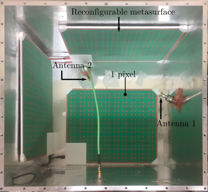
For our experiments we cover three contiguous and non-parallel walls of a metallic parallelepipedic cavity () with electronically reconfigurable metasurfaces (ERMs) 222The ERMs are placed on three contiguous and non-parallel cavity walls to avoid potentially non-generic modes. Gros et al. (2014a), without significantly altering the cavity geometry (see Fig. 1). Each of the three metasurfaces consists of phase-binary pixels. The underlying working principle of hybridizing two resonances is outlined in Ref. Kaina et al. (2014). By controlling the bias voltage of a PIN diode, each pixel can individually be configured to emulate the behavior of a quasi perfect electric or quasi perfect magnetic conductor. Stated differently, the phase of the tangential component of the field reflected by the pixel can be shifted by . Note that our proposal to locally modulate the cavity’s boundary conditions could also be implemented with other designs of tunable impedance surfaces, such as mushroom structures Sievenpiper et al. (2003); Sihvola (2007); Sleasman et al. (2016); Li et al. (2018). Since the design of our metasurface leverages resonant effects, the band of frequencies over which it displays the desired effect is a priori inherently limited. The ERM prototype we use for our experiments has been designed to work efficiently within a bandwidth around .
To evaluate whether boundary condition modulations induced by ERMs are able to create a chaotic cavity, we compare the statistical distribution of the normalized intensity of Cartesian field components measured for ensembles configurations of ERMs with the theoretical RMT distribution. The main steps leading to the RMT distribution of the normalized field intensity of an ensemble of responses resulting from stirring are given in the Supplemental Material (interested readers are referred to Gros et al. (2016, 2015b, 2018a) for details). We recall here only the final RMT prediction which reads
| (1) |
where is the phase rigidity,
| (2) |
is the Pnini and Shapiro distribution Pnini and Shapiro (1996); Gros et al. (2016); Kim et al. (2005) and is the phase rigidity distribution depending only on the mean modal overlap Gros et al. (2016, 2015b) (see Supplemental Material for an analytical expression). For a 3D electromagnetic cavity of volume , the mean density of states can be estimated with Weyl’s law, which reads at leading order 333In Weyl’s Law applied to a 3D EM cavity, there is no term proportional to and the total surface of the cavity; hence changing the configuration of an ERM is not expected to affect the cavity’s mean density of states.
| (3) |
where is the speed of light and the mean of the considered frequency window. The mean modal overlap is thus related to , , the modal width and the composite quality factor through
| (4) |
First, we are interested in the minimum number of metasurface pixels that have to emulate a perfect magnetic conductor to transform a regular metallic cavity into a chaotic one. To that end, we choose 500 random configurations of the three ERMs for which the overall number of PMC-like (’activated’) pixels, , is fixed and the remaining pixels are let in their PEC-like state (not ’activated’). For each configuration, we measure with a HP 8720D vector network analyzer the -parameters between two monopole antennas for 1601 frequency points in a frequency window of MHz around GHz where the pixels are the most efficient. This experiment is repeated for different value of . Then, for each set of experiments with fixed , we extract for both antennas their frequency-dependent coupling constants which readKuhl et al. (2013); Köber et al. (2010); Kuhl et al. (2017); Fyodorov et al. (2005):
| (5) |
where () are the reflection parameters and denotes an ensemble average over random ERM configurations. Then, we deduce from the measurement of the transmission parameter the normalized value of the amplitude of the Cartesian component of the electric field along the orientation of the monopole antenna 2 inside the cavity as Gros et al. (2015b)
| (6) |
where is the electric field at the position of antenna 2 and is the unit vector along the polarization of antenna 2. The RMT prediction in Eq. 11 assumes that is vanishing. Physically, this means that static contributions such as direct processes (short path) are negligible Baranger and Mello (1996); Hart et al. (2009); Yeh et al. (2010a, b); Dietz et al. (2010). Reasons for the presence of static contributions include directivity and relative positions of the antennas, as well as the ERMs’ stirring efficiency. To extract the universal properties from our experiments that can be compared with RMT predictions, we numerically suppress the non-universal static contribution via the commonly used transformation Dietz et al. (2010); Gradoni et al. (2014), where denotes averaging over ERM configurations 444 In practical applications involving reconfigurable wave chaos, such a differential approach to remove the static contribution is routinely used to efficiently use the available degrees of freedom del Hougne et al. (2016b, 2018b); del Hougne and Lerosey (2018); Yoya et al. (2018).. The universal and non-universal contributions in our data are discussed and displayed in detail in the Supplemental Material.
For each set of experiments with fixed , we compare the empirical cumulative distribution function (ECDF) of the normalized field intensity of the ensemble of cavity configurations, , with the theoretical cumulative distribution function
| (7) |
where we use the experimentally obtained value of . To estimate with Eq. 4, we extract from our data the cavity’s composite -factor as , where is the intensity decay time of the inverse Fourier transformed transmission signal . Around GHz, we thereby estimate .
The deviation of the measured ECDF of field intensity from the RMT prediction with is then estimated via the parameter defined as
| (8) |
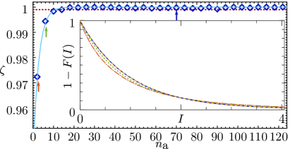
In Fig 2, we present the results. The diamonds () correspond to the experimentally obtained values of . A good agreement between the empirical and the RMT prediction is guaranteed as soon as . This is illustrated in the inset of Fig 2 with the ECDFs , , corresponding respectively to cases of , and . Among the three ECDFs shown, only corresponding to the case , is in good agreement with the RMT prediction . Finally, to estimate the minimum number of activated pixels, , required to obtain a chaotic cavity, we interpolate the measured by a heuristic function and search the value such that . The fit yields , and . Therefore, in the considered cavity, . This number depends obviously on the utilized metasurface design.
| label | ||||
|---|---|---|---|---|
| a) | ||||
| b) | ||||
| c) | ||||
| d) | ||||
| e) |
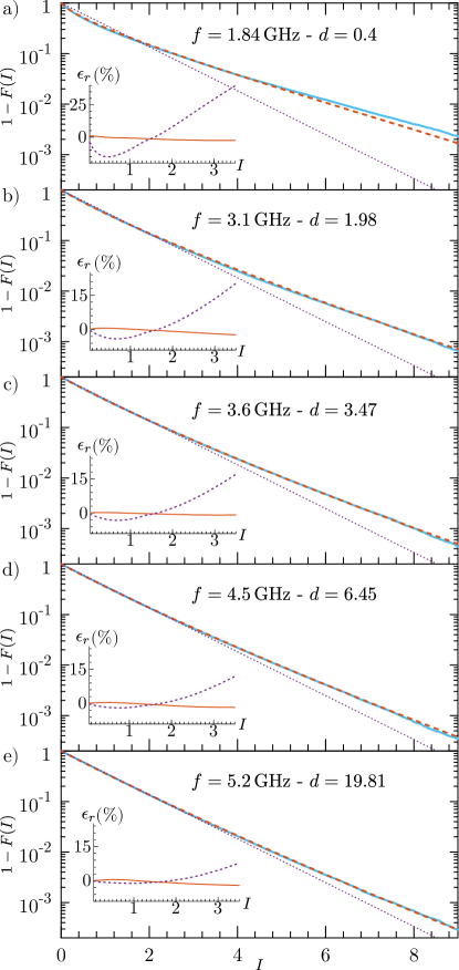
Having demonstrated that in a regular cavity equipped with ERMs chaotic behavior can be observed within the ERMs’ operation band, we now consider frequencies outside this band allowing us to explore different regimes of modal overlap. Indeed, although the ERM pixels are individually less efficient far outside their designed operating band (the phase difference between the two states is well below ), surprisingly we observe that collectively they are still able to sufficiently alter the boundary conditions to create wave-chaotic behavior. Hence we now choose 9000 fully random configurations of the 228 pixels. For each ERM configuration, we measure the -parameters between the monopole antennas for 1601 frequency points in . At this point, we draw the reader’s attention to the fact that most of RMT predictions assume that the mean density of state, the coupling strength of antenna, the absorption and the ensuing mean modal overlap are constantStöckmann (1999); Sokolov and Zelevinsky (1989); Kuhl et al. (2013); Köber et al. (2010); Savin et al. (2017); Gradoni et al. (2014); Gros et al. (2014a, 2015b); Kuhl et al. (2017); Fyodorov and Savin (2012); Gros et al. (2014b); Poli et al. (2012); Kumar et al. (2013); Dietz et al. (2010); Guhr et al. (1998). Practically, this means that we assume these quantities to vary only slightly within the investigated frequency range. Obviously, in the present study none of the above mentioned parameters are slightly varying on the full frequency range from GHz to GHz, especially the mean density of state. Therefore, we focus our study on a subset of five frequency windows of 150 MHz width, labeled a) to e) and respectively centered on GHz, GH., GHz, GHz and GHz. Table 1 indicates for each of these frequency windows the estimated composite -factor, the associated value of the modal overlap and the mode number of the cavity, given by . Then, we can study the field intensity distribution of the ensemble of cavity configurations, and hence the chaoticity, for different modal overlap regimes ranging from low modal overlap () around the 108th mode of the cavity to very high modal overlap () around its 2479th mode. For each frequency window in Table 1, we compare as before the measured ECDF of the normalized field intensity with the theoretical cumulative distribution function , given by Eq. 7, using the corresponding experimentally measured value of . The results are shown in Fig. 3 where the panels a)-e) correspond to frequency windows a)-e) in Table 1. In each panel of Fig. 3, the continuous blue curve, the dashed red curve and the purple dotted curve correspond, respectively, to the complementary ECDF, , of experimental data, the RMT prediction (equation 7) with given in Table 1, and the complementary cumulative distribution function for the Hill-Ericson-Schroeder regime Lemoine et al. (2007a); Hill (2009); Dietz et al. (2010); Mortessagne et al. (1993). The latter corresponds to the limit of very high modal overlap. From the very low modal overlap regime with around the mode of the cavity (Fig 3.a)) to the very high modal overlap regime with around the mode of the cavity (Fig 3.e)), we observe a very good agreement over three decades between the ECDF of the normalized field intensity of the ensemble of cavity’s configurations and the RMT prediction for chaotic cavities. Hence, the cavity in Fig. 1 displays the universal statistical behavior expected in chaotic cavities when we randomly modulate its boundary conditions.
In the EMC community, the idea to use an electronically reconfigurable reverberation chamber to stir the EM field was previously proposed Klingler (2005); Serra et al. (2017), but had not been experimentally demonstrated to date. More recently, it was proposed to used a metasurface to improve the field uniformity in a reverberation chamber Wanderlinder et al. (2017). The idea of improving field uniformity is closely related to that of making the cavity chaotic Gros et al. (2015a, b, 2014a). However, the metasurface used in Wanderlinder et al. (2017) is not reconfigurable. Consequently, unlike our ERMs, it cannot be used to simultaneously stir the EM field and improve the field uniformity. Finally, we note that the ECDF of the experimental data are increasingly close to the Hill-Ericson-Schroeder regime (dotted purple curves in Fig 3) as the modal overlap increases. Nevertheless, because of the large size of the statistical uncorrelated sample ( transmission parameters per frequency window 555Note that having an equivalent size of an uncorrelated statistical sample with mechanical stirring is much more difficult. Generally, the size of the statistical ensemble is between one and two orders of magnitude smaller. Lemoine et al. (2007b, a)) obtained by modulating the boundary condition of the cavity with ERMs, one can still discriminate between the RMT prediction and the Hill-Ericson-Schroeder regime — mainly on the tail of the distribution 666The difference between both distributions is also visible on the bulk of the probability distribution function (see insets of Fig 3). This is the case even for the largest modal overlap regime with studied here (Fig. 3.e).
In conclusion, we experimentally showed that random modulations of a regularly shaped cavity’s boundary conditions with simple metasurfaces constitute a new approach to construct a chaotic reverberation chamber without mechanical modifications. Here, we have demonstrated that this approach enables the observation of chaotic behavior for a wide range of modal overlap regimes, even at frequencies as low as the cavity mode. From a practical point of view, in a forthcoming publication Gros et al. (2018b), we will demonstrate how the metasurfaces can create a large number of uncorrelated cavity configurations which is an important features for many applications Lemoine et al. (2007b, a); Krauthauser et al. (2005); Lunden and Backstrom (2000); Gradoni et al. (2013); Sleasman et al. (2016); del Hougne and Lerosey (2018); Tondo Yoya et al. (2017); del Hougne et al. (2018b). From a more fundamental point of view, these reconfigurable chaotic cavities could be used to verify recent RMT predictions Savin et al. (2017); Fyodorov et al. (2017) due to the tantamount realizations they can produce easily and rapidly.
Acknowledgements.
The authors thank Olivier Legrand, Ulrich Kuhl and Fabrice Mortessagne from the Université Côte d’Azur for fruitful discussions and acknowledge funding from the French “Ministère des Armées, Direction Générale de l’Armement”.References
- Giannoni et al. (1991) M. J. Giannoni, A. Voros, and J. Zinn-Justin, eds., Les Houches 1989- Session LII: Chaos and quantum physics (North-Holland, 1991).
- Verbaarschot et al. (1985) J. J. M. Verbaarschot, H. A. Weidenmüller, and M. R. Zirnbauer, “Grassmann integration in stochastic quantum physics: The case of compound-nucleus scattering,” Phys. Rep. 129, 367–438 (1985).
- Berry (1977) M. V. Berry, “Regular and irregular semiclassical wavefunctions,” J. Phys. A. Math. Gen. 10, 2083–2091 (1977).
- Lombardi and Seligman (1993) M. Lombardi and T. H. Seligman, “Universal and nonuniversal statistical properties of levels and intensities for chaotic rydberg molecules,” Phys. Rev. A 47, 3571–3586 (1993).
- Mortessagne et al. (1993) F. Mortessagne, O. Legrand, and D. Sornette, “Transient chaos in room acoustics.” Chaos 3, 529–541 (1993).
- Aurégan and Pagneux (2016) Y. Aurégan and V. Pagneux, “Acoustic Scattering in Duct With a Chaotic Cavity,” Acta Acust. united with Acust. 102, 869–875 (2016).
- Tomsovic and Brown (2010) S. Tomsovic and M. G. Brown, “Ocean acoustics: A novel laboratory for wave chaos,” in New Directions in Linear Acoustics and Vibration; Quantum Chaos, Random Matrix Theory and Complexity, edited by M Wright and R Weaver (Cambridge University Press, 2010) Chap. 11, pp. 169–183.
- Lobkis and Weaver (2000) O. I. Lobkis and R. L. Weaver, “Complex modal statistics in a reverberant dissipative body,” The Journal of the Acoustical Society of America 108, 1480–1485 (2000).
- Doya et al. (2002) V. Doya, O. Legrand, F. Mortessagne, and C. Miniatura, “Speckle statistics in a chaotic multimode fiber,” Phys. Rev. E 65, 056223 (2002).
- Stöckmann and Stein (1990) H.-J. Stöckmann and J. Stein, “”Quantum” Chaos in Billiards Studied by Microwave Absorption,” Phys. Rev. Lett. 64, 2215–2218 (1990).
- Deus et al. (1995) S. Deus, P. M. Koch, and L. Sirko, “Statistical properties of the eigenfrequency distribution of three-dimensional microwave cavities,” Phys. Rev. E 52, 1146–1155 (1995).
- Kuhl et al. (2013) U. Kuhl, O. Legrand, and F. Mortessagne, “Microwave experiments using open chaotic cavities in the realm of the effective hamiltonian formalism,” Fortschritte der Physik 61, 404–419 (2013).
- Dietz and Richter (2015) B. Dietz and A. Richter, “Quantum and wave dynamical chaos in superconducting microwave billiards,” Chaos An Interdiscip. J. Nonlinear Sci. 25, 097601 (2015).
- Barthélemy et al. (2005) J. Barthélemy, O. Legrand, and F. Mortessagne, “Complete matrix in a microwave cavity at room temperature,” Phys. Rev. E 71, 016205 (2005).
- Bohigas et al. (1984) O. Bohigas, M. J. Giannoni, and C. Schmit, “Characterization of chaotic quantum spectra and universality of level fluctuation laws,” Phys. Rev. Lett. 52, 1–4 (1984).
- Stöckmann (1999) Hans-Jürgen Stöckmann, Quantum Chaos: An Introduction (Cambridge University Press, 1999).
- Guhr et al. (1998) T. Guhr, Axel Müller-Groeling, and Hans A. Weidenmüller, “Random-matrix theories in quantum physics: common concepts,” Phys. Rep. 299, 189–425 (1998).
- Sokolov and Zelevinsky (1989) V.V. Sokolov and V.G. Zelevinsky, “Dynamics and statistics of unstable quantum states,” Nucl. Phys. A 504, 562–588 (1989).
- Rotter (2009) I. Rotter, “A non-Hermitian Hamilton operator and the physics of open quantum systems,” J. Phys. A 42, 153001 (2009).
- Gros et al. (2016) J.-B. Gros, U. Kuhl, O. Legrand, and F. Mortessagne, “Lossy chaotic electromagnetic reverberation chambers: Universal statistical behavior of the vectorial field,” Phys. Rev. E 93, 032108 (2016).
- Gros et al. (2015a) J.-B. Gros, U. Kuhl, O. Legrand, F. Mortessagne, O. Picon, and E. Richalot, “Statistics of the electromagnetic response of a chaotic reverberation chamber,” Adv. Electromagn. 4, 38 (2015a), 1409.5863 .
- Gros et al. (2014a) J.-B. Gros, O. Legrand, F. Mortessagne, E. Richalot, and K. Selemani, “Universal behaviour of a wave chaos based electromagnetic reverberation chamber,” Wave Motion 51, 664–672 (2014a).
- Gradoni et al. (2014) G. Gradoni, J.-H. Yeh, B. Xiao, T. M. Antonsen, S. M. Anlage, and E. Ott, “Predicting the statistics of wave transport through chaotic cavities by the random coupling model: A review and recent progress,” Wave Motion 51, 606–621 (2014), arXiv:1303.6526v1 .
- Bastianelli et al. (2017) L. Bastianelli, G. Gradoni, F. Moglie, and V. M. Primiani, “Full wave analysis of chaotic reverberation chambers,” in 2017 XXXIInd Gen. Assem. Sci. Symp. Int. Union Radio Sci. (URSI GASS), August (IEEE, 2017) pp. 1–4.
- Arnaut (2001) L. R. Arnaut, “Operation of electromagnetic reverberation chambers with wave diffractors at relatively low frequencies,” IEEE Trans. Electromagn. Compat. 43, 637–653 (2001).
- Sarrazin and Richalot (2017) F. Sarrazin and E. Richalot, “Cavity modes inside a mode-stirred reverberation chamber extracted using the matrix pencil method,” in 2017 11th European Conference on Antennas and Propagation (EUCAP) (2017) pp. 620–622.
- Orjubin et al. (2009) G. Orjubin, E. Richalot, O. Picon, and O. Legrand, “Wave chaos techniques to analyze a modeled reverberation chamber,” Comptes Rendus Phys. 10, 42–53 (2009).
- Kaina et al. (2015) N. Kaina, M. Dupré, G. Lerosey, and M. Fink, “Shaping complex microwave fields in reverberating media with binary tunable metasurfaces,” Sci. Rep. 4, 6693 (2015).
- Dupré et al. (2015) M. Dupré, P. del Hougne, M. Fink, F. Lemoult, and G. Lerosey, “Wave-Field Shaping in Cavities: Waves Trapped in a Box with Controllable Boundaries,” Phys. Rev. Lett. 115, 017701 (2015).
- del Hougne et al. (2016a) P. del Hougne, F. Lemoult, M. Fink, and G. Lerosey, “Spatiotemporal wave front shaping in a microwave cavity,” Phys. Rev. Lett. 117, 134302 (2016a).
- Sleasman et al. (2016) T. Sleasman, M. F. Imani, J. N. Gollub, and D. R. Smith, “Microwave Imaging Using a Disordered Cavity with a Dynamically Tunable Impedance Surface,” Phys. Rev. Appl. 6, 054019 (2016).
- Tondo Yoya et al. (2017) A. C. Tondo Yoya, B. Fuchs, and M. Davy, “Computational passive imaging of thermal sources with a leaky chaotic cavity,” Appl. Phys. Lett. 111, 193501 (2017).
- Asefi and LoVetri (2017) M. Asefi and J. LoVetri, “Use of field-perturbing elements to increase nonredundant data for microwave imaging systems,” IEEE Trans. Microwave Theory Tech. 65, 3172–3179 (2017).
- Yoya et al. (2018) A. C. T. Yoya, B. Fuchs, and M. Davy, “A reconfigurable chaotic cavity with fluorescent lamps for microwave computational imaging,” arXiv preprint arXiv:1810.07099 (2018).
- del Hougne et al. (2017) P. del Hougne, M. Fink, and G. Lerosey, “Shaping Microwave Fields Using Nonlinear Unsolicited Feedback: Application to Enhance Energy Harvesting,” Phys. Rev. Appl. 8, 061001 (2017), 1706.00450 .
- del Hougne et al. (2019) P. del Hougne, M. Fink, and G. Lerosey, “Optimally diverse communication channels in disordered environments with tuned randomness,” Nat. Electron. 2, 36 (2019).
- del Hougne et al. (2018a) P. del Hougne, M. F. Imani, T. Sleasman, J. N. Gollub, M. Fink, G. Lerosey, and D. R Smith, “Dynamic Metasurface Aperture as Smart Around-the-Corner Motion Detector,” Sci. Rep. 8, 6536 (2018a).
- del Hougne et al. (2018b) P. del Hougne, M. F. Imani, M. Fink, D. R. Smith, and G. Lerosey, “Precise localization of multiple noncooperative objects in a disordered cavity by wave front shaping,” Phys. Rev. Lett. 121, 063901 (2018b).
- Davy et al. (2016) M. Davy, J. de Rosny, and P. Besnier, “Green’s function retrieval with absorbing probes in reverberating cavities,” Phys. Rev. Lett. 116, 213902 (2016).
- del Hougne and Lerosey (2018) P. del Hougne and G. Lerosey, “Leveraging chaos for wave-based analog computation: Demonstration with indoor wireless communication signals,” Phys. Rev. X 8, 041037 (2018).
- Note (1) The field ergodicity means that fields in chaotic systems are statistically equivalent to an appropriate random superposition of plane waves leading to a field which is statistically uniform,depolarized, and isotropic i.e the fields are speckle-like Gros et al. (2016, 2015b); Pnini and Shapiro (1996); Dörr et al. (1998); Kim et al. (2005); Hemmady et al. (2005).
- Kuhl et al. (2017) U. Kuhl, O. Legrand, F. Mortessagne, K. Oubaha, and M. Richter, “Statistics of Reflection and Transmission in the Strong Overlap Regime of Fully Chaotic Reverberation Chambers,” in EUMCWeek 2017 Nürnberg. (2017) pp. 1–4, arXiv:1706.04873 .
- Serra et al. (2017) R. Serra, A. C. Marvin, F. Moglie, V. M. Primiani, A. Cozza, L. R. Arnaut, Y. Huang, M. O. Hatfield, M. Klingler, and F. Leferink, “Reverberation chambers a la carte: An overview of the different mode-stirring techniques,” IEEE Electromagnetic Compatibility Magazine 6, 63–78 (2017).
- Hill (2009) D. A. Hill, Electromagnetic fields in cavities: deterministic and statistical theories, IEEE Press Series on Electromagnetic Wave Theory (IEEE ; Wiley, 2009).
- Gros et al. (2015b) J.-B Gros, U. Kuhl, O. Legrand, F. Mortessagne, and E. Richalot, “Universal intensity statistics in a chaotic reverberation chamber to refine the criterion of statistical field uniformity,” in 2015 IEEE Metrology for Aerospace (MetroAeroSpace) (2015) pp. 225–229.
- Cozza (2011) A. Cozza, “The Role of Losses in the Definition of the Overmoded Condition for Reverberation Chambers and Their Statistics,” IEEE Trans. Electromagn. Compat. 53, 296–307 (2011).
- Schroeder and Kuttruff (1962) M. R. Schroeder and K. H. Kuttruff, “On frequency response curves in rooms. Comparison of experimental, theoretical, and Monte Carlo results for the average frequency spacing between maxima,” J. Acoust. Soc. … 34, 76 (1962).
- Note (2) The ERMs are placed on three contiguous and non-parallel cavity walls to avoid potentially non-generic modes. Gros et al. (2014a).
- Kaina et al. (2014) N. Kaina, M. Dupré, M. Fink, and G. Lerosey, “Hybridized resonances to design tunable binary phase metasurface unit cells,” Opt. Express 22, 18881–18888 (2014).
- Sievenpiper et al. (2003) D. F. Sievenpiper, J. H. Schaffner, H. J. Song, R. Y. Loo, and G. Tangonan, “Two-dimensional beam steering using an electrically tunable impedance surface,” IEEE Trans. Antennas Propag. 51, 2713–2722 (2003).
- Sihvola (2007) A. Sihvola, “Metamaterials in electromagnetics,” Metamaterials 1, 2–11 (2007).
- Li et al. (2018) A. Li, S. Singh, and D. Sievenpiper, “Metasurfaces and their applications,” Nanophotonics 7, 989–1011 (2018).
- Gros et al. (2018a) J.-B. Gros, U. Kuhl, O. Legrand, F. Mortessagne, and E. Richalot, “Review on chaotic reverberation chambers : theory and experiment,” in preparation (2018a).
- Pnini and Shapiro (1996) R. Pnini and B. Shapiro, “Intensity fluctuations in closed and open systems,” Phys. Rev. E 54, R1032–R1035 (1996).
- Kim et al. (2005) Y.-H. Kim, Ulrich Kuhl, H.-J. Stöckmann, and P. W. Brouwer, “Measurement of Long-Range Wave-Function Correlations in an Open Microwave Billiard,” Phys. Rev. Lett. 94, 036804 (2005).
- Note (3) In Weyl’s Law applied to a 3D EM cavity, there is no term proportional to and the total surface of the cavity; hence changing the configuration of an ERM is not expected to affect the cavity’s mean density of states.
- Köber et al. (2010) B. Köber, U. Kuhl, H.-J. Stöckmann, T. Gorin, D. V. Savin, and T. H. Seligman, “Microwave fidelity studies by varying antenna coupling,” Phys. Rev. E 82, 036207 (2010).
- Fyodorov et al. (2005) Y. V. Fyodorov, D. V. Savin, and H.-J. Sommers, “Scattering, reflection and impedance of waves in chaotic and disordered systems with absorption,” J. Phys. A. Math. Gen. 38, 10731–10760 (2005).
- Baranger and Mello (1996) H. U. Baranger and P. A. Mello, “Short paths and information theory in quantum chaotic scattering: transport through quantum dots,” Europhys. Lett. 33, 465–470 (1996).
- Hart et al. (2009) J. A. Hart, T. M. Antonsen, and E. Ott, “Effect of short ray trajectories on the scattering statistics of wave chaotic systems,” Phys. Rev. E 80, 041109 (2009).
- Yeh et al. (2010a) J.-H. Yeh, J. Hart, E. Bradshaw, T. M. Antonsen, E. Ott, and S. M. Anlage, “Experimental examination of the effect of short ray trajectories in two-port wave-chaotic scattering systems,” Phys. Rev. E 82, 041114 (2010a).
- Yeh et al. (2010b) J.-H. Yeh, J. A. Hart, E. Bradshaw, T. M. Antonsen, E. Ott, and S. M. Anlage, “Universal and nonuniversal properties of wave-chaotic scattering systems,” Phys. Rev. E 81, 025201 (2010b).
- Dietz et al. (2010) B. Dietz, H.L. Harney, A. Richter, F. Schäfer, and H.A. Weidenmüller, “Cross-section fluctuations in chaotic scattering,” Phys. Lett. B 685, 263–269 (2010).
- Note (4) In practical applications involving reconfigurable wave chaos, such a differential approach to remove the static contribution is routinely used to efficiently use the available degrees of freedom del Hougne et al. (2016b, 2018b); del Hougne and Lerosey (2018); Yoya et al. (2018).
- Savin et al. (2017) D. V. Savin, M. Richter, U. Kuhl, O. Legrand, and F. Mortessagne, “Fluctuations in an established transmission in the presence of a complex environment,” Phys. Rev. E 96, 032221 (2017).
- Fyodorov and Savin (2012) Y. V. Fyodorov and D. V. Savin, “Statistics of Resonance Width Shifts as a Signature of Eigenfunction Nonorthogonality,” Phys. Rev. Lett. 108, 184101 (2012).
- Gros et al. (2014b) J.-B. Gros, U. Kuhl, O. Legrand, F. Mortessagne, E. Richalot, and D. V. Savin, “Experimental width shift distribution: A test of nonorthogonality for local and global perturbations,” Phys. Rev. Lett. 113, 224101 (2014b).
- Poli et al. (2012) C. Poli, G Luna-Acosta, and H.-J. Stöckmann, “Nearest Level Spacing Statistics in Open Chaotic Systems: Generalization of the Wigner Surmise,” Phys. Rev. Lett. 108, 174101 (2012).
- Kumar et al. (2013) S. Kumar, A. Nock, H.-J. Sommers, T. Guhr, B Dietz, M. Miski-Oglu, Achim Richter, and F. Schäfer, “Distribution of Scattering Matrix Elements in Quantum Chaotic Scattering,” Phys. Rev. Lett. 111, 030403 (2013).
- Lemoine et al. (2007a) C. Lemoine, P. Besnier, and M. Drissi, “Investigation of Reverberation Chamber Measurements Through High-Power Goodness-of-Fit Tests,” IEEE Trans. Electromagn. Compat. 49, 745–755 (2007a).
- Klingler (2005) M. Klingler, “Dispositif et procédé de brassage électromagnétique dans une chambre réverbérante à brassage de modes,” Patent FR 2 887 337 (2005).
- Wanderlinder et al. (2017) L. F. Wanderlinder, D. Lemaire, I. Coccato, and D. Seetharamdoo, “Practical implementation of metamaterials in a reverberation chamber to reduce the luf,” in 2017 IEEE 5th International Symposium on Electromagnetic Compatibility (EMC-Beijing) (2017) pp. 1–3.
- Note (5) Note that having an equivalent size of an uncorrelated statistical sample with mechanical stirring is much more difficult. Generally, the size of the statistical ensemble is between one and two orders of magnitude smaller. Lemoine et al. (2007b, a).
- Note (6) The difference between both distributions is also visible on the bulk of the probability distribution function (see insets of Fig 3).
- Gros et al. (2018b) J.-B. Gros, P. del Hougne, U. Kuhl, O. Legrand, F. Mortessagne, and G. Lerosey, “Mode-stirring in a chaotic cavity by reconfiguring its boundaries with tunable metasurfaces,” in preparation (2018b).
- Lemoine et al. (2007b) C. Lemoine, P. Besnier, and M. Drissi, “Advanced method for estimating number of independent samples available with stirrer in reverberation chamber,” Electronics Letters 43, 861–862 (2007b).
- Krauthauser et al. (2005) H. G. Krauthauser, T. Winzerling, J. Nitsch, N. Eulig, and A. Enders, “Statistical interpretation of autocorrelation coefficients for fields in mode-stirred chambers,” in 2005 International Symposium on Electromagnetic Compatibility, 2005. EMC 2005., Vol. 2 (2005) pp. 550–555.
- Lunden and Backstrom (2000) O. Lunden and M. Backstrom, “Stirrer efficiency in foa reverberation chambers. evaluation of correlation coefficients and chi-squared tests,” in IEEE International Symposium on Electromagnetic Compatibility. Symposium Record (Cat. No.00CH37016), Vol. 1 (2000) pp. 11–16 vol.1.
- Gradoni et al. (2013) G. Gradoni, V. Mariani Primiani, and F. Moglie, “Reverberation Chamber as a Multivariate Process: Fdtd Evaluation of Correlation Matrix and Independent Positions,” Prog. Electromagn. Res. 133, 217–234 (2013).
- Fyodorov et al. (2017) Y. V. Fyodorov, S. Suwunnarat, and T. Kottos, “Distribution of zeros of the -matrix of chaotic cavities with localized losses and coherent perfect absorption: non-perturbative results,” Journal of Physics A: Mathematical and Theoretical 50, 30LT01 (2017).
- Dörr et al. (1998) U. Dörr, H.-J. Stöckmann, M. Barth, and U. Kuhl, “Scarred and chaotic field distributions in a three-dimensional Sinai-microwave resonator,” Phys. Rev. Lett. 80, 1030–1033 (1998).
- Hemmady et al. (2005) S. Hemmady, X. Zheng, T. M. Antonsen Jr, E. Ott, and S. M. Anlage, “Universal statistics of the scattering coefficient of chaotic microwave cavities,” Phys. Rev. E 71, 056215 (2005).
- del Hougne et al. (2016b) P. del Hougne, B. Rajaei, L. Daudet, and G. Lerosey, “Intensity-only measurement of partially uncontrollable transmission matrix: demonstration with wave-field shaping in a microwave cavity,” Opt. Express 24, 18631–18641 (2016b).
I Supplemental Material:
Wave Chaos in a Cavity of Regular Geometry with Tunable Boundaries
I.1 Universal versus non universal behaviors
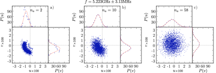
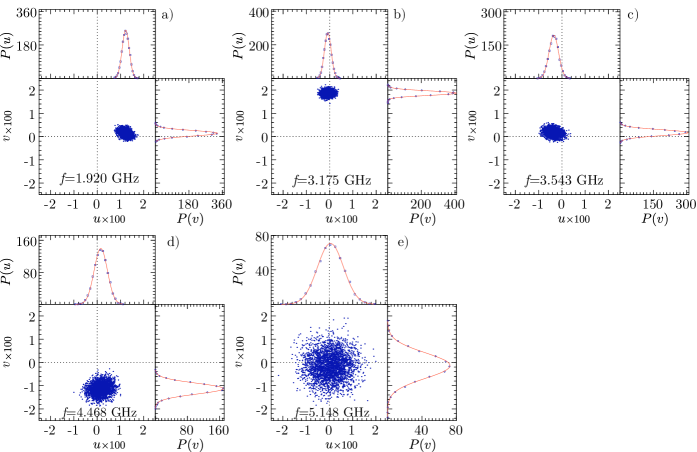
In a chaotic cavity, the only universal statistical requirement for the field is that its real and imaginary parts are Normally distributed. Therefore, this property can be used as an indicator of the efficiency of the reconfigurable metasurface to make the cavity chaotic. As illustrated in the Fig 4 and Fig 6, the Gaussianity of real and imaginary parts of the field is systemically verified in our experiments each time the metasurfaces configurations sufficiently impact the boundary conditions of the regular cavity. Indeed, only the case shown in Fig 4.a), corresponding to frequencies inside the design operation band of the metasurface but an ensemble of configurations where the number of activated pixels of the metasurface are to small (only two), does not agree with the universal behavior of a chaotic cavity.
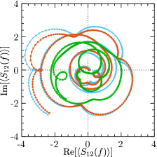
The field in chaotic cavities can also display some non universal statistics, which are not related to the chaotic nature of the cavity but are experiment-dependent features. For instance, we observed non vanishing mean values of the complex field (see Fig 4, Fig 5 and Fig 6). In our experiments the latter can be explained by non negligible direct processes (short path effects) which mainly stem from the directivity and relative antenna positions. This is illustrated in Fig 6 where the mean values of the complex fields over metasurface configurations follow continuous and rotating trajectory in the complex plane when the frequency increases.
I.2 Random matrix prediction of the normalized field intensity of a chaotic cavity
We briefly recall here the main steps leading to this prediction (for details, interested readers can refer to Gros et al. (2016, 2015b, 2018a)). In presence of losses, for a given configuration of an ideally chaotic cavity (or a given frequency, relying on ergodicity), the real and imaginary parts of each Cartesian component of the field are independently Gaussian distributed, but with different variances Gros et al. (2016, 2014a). The ensuing distribution of the modulus square of each component depends on a single parameter , called the phase rigidity, defined by Gros et al. (2016):
| (9) |
More precisely, in a chaotic RC, due to the ergodicity of the modes contributing to the response, for a given excitation frequency and a given configuration (here ERMs configurations, polarisations and positions of the antennas), the probability distribution of the normalized intensity of the Cartesian component depends solely on the modulus of and is given by Kim et al. (2005); Gros et al. (2016).
| (10) |
with being the modified Bessel function of the first kind. This result was originally proposed by Pnini and Shapiro Pnini and Shapiro (1996) to model the statistics of scalar fields in partially open chaotic systems. Note that the above distribution continuously interpolates between the two extreme distributions, namely Porter-Thomas for lossless closed systems () and exponential for completely open systems ( ). The latter case corresponds to the limit where the field is statistically equivalent to a random superposition of traveling plane waves Pnini and Shapiro (1996); Gros et al. (2016) meaning that real and imaginary parts of each Cartesian components of the field are statistically independent and identically distributed following a normal distribution. This regime is know as the Hill’s regime in the EMC community Lemoine et al. (2007a); Hill (2009) , the Ericson’s regime in nuclear physics Dietz et al. (2010) or Schroeder’s regime in room acoustics Mortessagne et al. (1993) and corresponds to a very high modal overlap regime. Since the phase rigidity is itself a distributed quantity, the distribution of the normalized field intensity in a chaotic reverberation chamber for an ensemble of responses resulting from stirring reads
| (11) |
where is the distribution of the phase rigidity of the responses. Preliminary investigations, based on numerical simulations of the Random Matrix model described in Gros et al. (2016), show that depends only on the mean modal overlap . An Antsatz was proposed in Gros et al. (2015b) to determine from the only knowledge of . This Ansatz reads:
| (12) |
where the parameter has a smooth -dependence Gros et al. (2015b) numerically deduced from our RMT model presented in Gros et al. (2016). Originally in Gros et al. (2015b) , the empirical estimation of was limited to . Currently, have been extended to larger values of and is given by Gros et al. (2018a)
| (13) |
with , and Gros et al. (2018a).