pizza: an open-source pseudo-spectral code for spherical quasi-geostrophic convection–B

pizza: an open-source pseudo-spectral code for spherical quasi-geostrophic convection

We present a new pseudo-spectral open-source code nicknamed pizza. It is dedicated to the study of rapidly-rotating Boussinesq convection under the 2-D spherical quasi-geostrophic approximation, a physical hypothesis that is appropriate to model the turbulent convection that develops in planetary interiors. The code uses a Fourier decomposition in the azimuthal direction and supports both a Chebyshev collocation method and a sparse Chebyshev integration formulation in the cylindrically-radial direction. It supports several temporal discretisation schemes encompassing multi-step time steppers as well as diagonally-implicit Runge-Kutta schemes. The code has been tested and validated by comparing weakly-nonlinear convection with the eigenmodes from a linear solver. The comparison of the two radial discretisation schemes has revealed the superiority of the Chebyshev integration method over the classical collocation approach both in terms of memory requirements and operation counts. The good parallelisation efficiency enables the computation of large problem sizes with $\mathcal{O}(10^{4}\times 10^{4})$ grid points using several thousands of ranks. This allows the computation of numerical models in the turbulent regime of quasi-geostrophic convection characterised by large Reynolds $Re$ and yet small Rossby numbers $Ro$. A preliminary result obtained for a strongly supercritical numerical model with a small Ekman number of $10^{-9}$ and a Prandtl number of unity yields $Re\simeq 10^{5}$ and $Ro\simeq 10^{-4}$. pizza is hence an efficient tool to study spherical quasi-geostrophic convection in a parameter regime inaccessible to current global 3-D spherical shell models.

1 Introduction

Convection under rapid rotation is ubiquitous in astrophysical bodies. The liquid iron cores of terrestrial planets or the atmospheres of the gas giants are selected examples where turbulent convection is strongly influenced by rotational effects (e.g. Aurnou et al., 2015). Such turbulent flows are characterised by very large Reynolds numbers $Re>10^{8}$ and yet small Rossby numbers $Ro<10^{-5}$, $Ro$ being defined as the ratio between the rotation period and the convective overturn time. This specific combination of $Re\gg 1$ and $Ro\ll 1$ corresponds to the so-called turbulent quasi-geostrophic regime of rotating convection (e.g. Julien et al., 2012; Stellmach et al., 2014). This implies that, in absence of a magnetic field, the pressure gradients balance the Coriolis force at leading order. As a consequence, the convective flow shows a pronounced invariance along the axis of rotation. At onset of rotating convection for instance, the flow pattern takes the form of quasi-geostrophic elongated columnar structures that have a typical size of $E^{1/3}$, where $E=\nu/\Omega d^{2}$ is the Ekman number with $\nu$ the kinematic viscosity, $\Omega$ the rotation frequency and $d$ the thickness of the convective layer (e.g. Busse, 1970; Dormy et al., 2004). Convection in natural objects corresponds to extremely small Ekman numbers with for instance $E\simeq 10^{-15}$ in the Earth core or $E\simeq 10^{-18}$ in the gas giants. The quasi-geostrophy of the convective flow is expected to hold as long as the dynamics is dominated by rotation, or in other words as long as the buoyancy force remains relatively small compared to the Coriolis force (Gilman, 1977; Julien et al., 2012; King et al., 2013; Cheng et al., 2015; Horn & Shishkina, 2015; Gastine et al., 2016).

Many laboratory experiments of rotating convection in spherical geometry have been carried out, either under micro-gravity conditions (e.g. Hart et al., 1986; Egbers et al., 2003); or on the ground using the centrifugal force as a surrogate of the radial distribution of buoyancy (e.g. Busse & Carrigan, 1974; Sumita & Olson, 2003; Shew & Lathrop, 2005). Because of their limited size, those experiments could only reach $E\simeq 5\times 10^{-6}$, far from the geophysical/astrophysical regime. In complement to the laboratory experiments, rotating convection in spherical geometry can also be studied by means of three-dimensional global numerical simulations. Because of computational limitations, those numerical models are currently limited to $E\gtrsim 10^{-7}$, $Re\lesssim 10^{4}$ and $Ro\gtrsim 10^{-3}$, hardly scratching into the turbulent quasi-geostrophic (hereafter QG) regime (Gastine et al., 2016; Schaeffer et al., 2017). Reaching lower Ekman numbers is hence mandatory to further explore this regime with $Re\gg 1$ and $Ro\ll 1$.

A way to alleviate the computational constraints inherent in global 3-D computations is to consider a spherical QG approximation of the convective flow (e.g. Busse & Or, 1986; Cardin & Olson, 1994; Plaut & Busse, 2002; Aubert et al., 2003; Morin & Dormy, 2004; Gillet & Jones, 2006; Calkins et al., 2012; Teed et al., 2012; Guervilly & Cardin, 2017; More & Dumberry, 2018) . The underlying assumption of the spherical QG approximation is that the leading-order cylindrically-radial and azimuthal velocity components are invariant along the axis of rotation $z$. Under this approximation, the variations of the axial vorticity along the rotation axis are also neglected and an averaging of the continuity equation along the rotation axis implies a linear dependence of the axial velocity on $z$ (Schaeffer & Cardin, 2005a; Gillet & Jones, 2006). The spherical QG approximation hence restricts the computation of the evolution of the convective velocity to two dimensions only. This is a limitation compared to the 3-D QG convective models developed by Calkins et al. (2013) which allow spatial modulations of the convective features along the rotation axis. Because of the radial distribution of the buoyancy forcing in spherical geometry, the temperature is not necessarily well-described by the quasi-geostrophic approximation. Spherical QG models with either a three-dimensional or a two-dimensional treatment of the temperature however yield very similar results (Guervilly & Cardin, 2016). Despite those approximations, the different implementations of the 2-D spherical QG models (e.g. Aubert et al., 2003; Gillet & Jones, 2006; Calkins et al., 2012; Teed et al., 2012; Guervilly & Cardin, 2017) have been found to compare favourably to 3-D direct numerical simulations in spherical geometry (e.g. Aubert et al., 2003; Schaeffer & Cardin, 2005a; Plaut et al., 2008). This indicates that such 2-D spherical QG models could be efficiently used to explore the turbulent QG regime of convection with $E<10^{-8}$ and $Re\gtrsim 10^{5}$, a parameter regime currently inaccessible to 3-D computations. Quasi-geostrophy is expected to hold as long as the dynamics is dominated by rotation, or in other words as long as the buoyancy force remains relatively small compared to the Coriolis force (Gilman, 1977; Julien et al., 2012; King et al., 2013; Cheng et al., 2015; Horn & Shishkina, 2015; Gastine et al., 2016).

The spatial discretisation strategy adopted in spherical QG models usually relies on a hybrid scheme with a truncated Fourier expansion in the azimuthal direction $\phi$ and second-order finite differences in the cylindrically-radial direction $s$ (e.g. Aubert et al., 2003; Calkins et al., 2012). Note that Brummell & Hart (1993) and Teed et al. (2012) rather employed a spectral Chebyshev collocation technique in $s$ but in the case of a cartesian QG model. The vast majority of those numerical codes adopt a pseudo-spectral approach where the nonlinear terms are treated in the physical space and time-advanced with an explicit Adams–Bashforth time scheme, while the linear terms are time-advanced in the Fourier space using a Crank–Nicolson scheme. In contrast to 3-D models where several codes with active on-going developments are freely accessible to the community (see Matsui et al., 2016), there is a no open-source code for spherical QG convection available to the community.

The purpose of this study is precisely to introduce a new open-source pseudo-spectral spherical QG code, nicknamed pizza. pizza is available at https://github.com/magic-sph/pizza as a free software that can be used, modified, and redistributed under the terms of the GNU GPL v3 license. The package also comes with a suite of python classes to allow a full analysis of the outputs and diagnostics produced by the code during its execution. The code, written in Fortran, uses a Fourier decomposition in $\phi$ and either a Chebyshev collocation or a sparse Chebyshev integration method in $s$ (e.g. Stellmach & Hansen, 2008; Muite, 2010; Marti et al., 2016). It supports a broad variety of implicit-explicit time schemes encompassing multi-step methods (e.g. Ascher et al., 1995) and implicit Runge-Kutta schemes (e.g. Ascher et al., 1997). The parallelisation strategy relies on the Message Passing Interface (MPI) library.

The paper is organised as follows. Section 2 presents the equations for spherical QG convection. Section 3 and 4 are dedicated to the spatial and temporal discretisation schemes implemented in pizza. The parallelisation strategy is described in section 5. The code validation and several examples are discussed in section 6 before concluding in section 7.

2 A quasi-geostrophic model of convection

Because of the strong axial invariance of the flow under rapid rotation, the QG models approximate 3-D convection in spherical geometry by a 2-D fluid domain which corresponds to the equatorial plane of a spherical shell. Using the cylindrical coordinates $(s,\phi,z)$, the QG fluid domain hence corresponds to an annulus of inner radius $s_{i}$ and outer radius $s_{o}$ rotating against the $z$-axis with an angular frequency $\Omega$. In the following, we adopt a dimensionless formulation of the spherical QG equations using the annulus gap $d=s_{o}-s_{i}$ as a reference length scale and the viscous diffusion time $d^{2}/\nu$ as the reference time scale. The temperature contrast $\Delta T$ between both boundaries defines the temperature scale. Gravity is assumed to grow linearly with the cylindrical radius $s$ and is non-dimensionalised using its value at the external radius $g_{o}$.

The formulation of the QG model implemented in pizza is based on the spherical QG approximation introduced by Busse & Or (1986) and further expanded by Aubert et al. (2003) and Gillet & Jones (2006) to include the effects of Ekman pumping. Following Schaeffer & Cardin (2005a) and Gillet & Jones (2006) the axial velocity $u_{z}$ is assumed to vary linearly with $z$. Under this assumption, the Boussinesq continuity equation under the spherical QG approximation yields

$$\dfrac{1}{s}\dfrac{\partial(su_{s})}{\partial s}+\dfrac{1}{s}\dfrac{\partial u_{\phi}}{\partial\phi}+\beta u_{s}=0\,,$$ (1)

where

$$\beta=\dfrac{1}{h}\dfrac{\mathrm{d}h}{\mathrm{d}s}=-\dfrac{s}{h^{2}}\,,$$ (2)

and $h=(s_{o}^{2}-s^{2})^{1/2}$ is half the height of the geostrophic cylinder at the cylindrical radius $s$. We adopt a vorticity-streamfunction formulation to fulfill the QG continuity equation (1). The cylindrically-radial and azimuthal velocity components are hence expanded as follows

$$u_{s}=\dfrac{1}{s}\dfrac{\partial\psi}{\partial\phi},\quad u_{\phi}=\overline{u_{\phi}}-\dfrac{\partial\psi}{\partial s}-\beta\psi,$$ (3)

where the streamfunction $\psi$ accounts for the non-axisymmetric motions, while $\overline{u_{\phi}}$ corresponds to the axisymmetric zonal flow component, the overbar denoting an azimuthal average. The axial vorticity $\omega$ is then expressed by

$$\omega=\dfrac{1}{s}\dfrac{\partial(s\overline{u_{\phi}})}{\partial s}-\mathcal{L}_{\beta}\psi,$$ (4)

where the operator $\mathcal{L}_{\beta}$ is defined by

$$\mathcal{L}_{\beta}\psi=\Delta\psi+\dfrac{1}{s}\dfrac{\partial(\beta s\psi)}{\partial s}\,.$$

In the above equation, $\Delta$ is the Laplacian operator in cylindrical coordinates. Under the QG approximation, the time evolution of the axial vorticity becomes

$$\dfrac{\partial\omega}{\partial t}+\mathchoice{\mbox{\boldmath$\displaystyle\nabla$}}{\mbox{\boldmath$\textstyle\nabla$}}{\mbox{\boldmath$\scriptstyle\nabla$}}{\mbox{\boldmath$\scriptscriptstyle\nabla$}}\cdot\left(\mathchoice{\mbox{\boldmath$\displaystyle u$}}{\mbox{\boldmath$\textstyle u$}}{\mbox{\boldmath$\scriptstyle u$}}{\mbox{\boldmath$\scriptscriptstyle u$}}\,\omega\right)=\dfrac{2}{E}\beta u_{s}-\dfrac{Ra}{Pr}\dfrac{1}{s_{o}}\dfrac{\partial\vartheta}{\partial\phi}+\mathcal{F}(E,\mathchoice{\mbox{\boldmath$\displaystyle u$}}{\mbox{\boldmath$\textstyle u$}}{\mbox{\boldmath$\scriptstyle u$}}{\mbox{\boldmath$\scriptscriptstyle u$}},\omega)+\Delta\omega\,,$$ (5)

where $\vartheta$ denotes the temperature perturbation. The reader is referred to Gillet & Jones (2006) for a comprehensive derivation of this equation. In the above equation, $\mathcal{F}(E,\mathchoice{\mbox{\boldmath$\displaystyle u$}}{\mbox{\boldmath$\textstyle u$}}{\mbox{\boldmath$\scriptstyle u$}}{\mbox{\boldmath$\scriptscriptstyle u$}},\omega)$ corresponds to the Ekman-pumping contribution (Schaeffer & Cardin, 2005a) to non-axisymmetric motions expressed by

$$\mathcal{F}(E,\mathchoice{\mbox{\boldmath$\displaystyle u$}}{\mbox{\boldmath$\textstyle u$}}{\mbox{\boldmath$\scriptstyle u$}}{\mbox{\boldmath$\scriptscriptstyle u$}},\omega)=-\Upsilon\left[\omega-\dfrac{\beta}{2}u_{\phi}+\beta\left(\dfrac{\partial}{\partial\phi}-\dfrac{5s_{o}}{2h}\right)u_{s}\right]\,.$$ (6)

where

$$\Upsilon=\left(\dfrac{s_{o}}{E}\right)^{1/2}\dfrac{1}{(s_{o}^{2}-s^{2})^{3/4}}\,.$$

To ensure a correct force balance in the azimuthal direction, the axial vorticity equation (5) is supplemented by an equation dedicated to the axisymmetric motions (Plaut & Busse, 2002). Taking a $\phi$-average of the azimuthal component of the Navier-Stokes equations yields

$$\dfrac{\partial\overline{u_{\phi}}}{\partial t}+\overline{u_{s}\omega}=-\Upsilon\,\overline{u_{\phi}}+\Delta\overline{u_{\phi}}-\dfrac{\overline{u_{\phi}}}{s^{2}}\,,$$ (7)

where the first term in the right-hand-side corresponds to the Ekman-pumping contribution for the axisymmetric motions (Aubert et al., 2003). The governing equations for the temperature perturbation under the QG approximation is given by

$$\dfrac{\partial\vartheta}{\partial t}+\mathchoice{\mbox{\boldmath$\displaystyle\nabla$}}{\mbox{\boldmath$\textstyle\nabla$}}{\mbox{\boldmath$\scriptstyle\nabla$}}{\mbox{\boldmath$\scriptscriptstyle\nabla$}}\cdot\left(\mathchoice{\mbox{\boldmath$\displaystyle u$}}{\mbox{\boldmath$\textstyle u$}}{\mbox{\boldmath$\scriptstyle u$}}{\mbox{\boldmath$\scriptscriptstyle u$}}\,\vartheta\right)+\beta u_{s}\vartheta+u_{s}\dfrac{\mathrm{d}T_{c}}{\mathrm{d}s}=\dfrac{1}{Pr}\Delta\vartheta\,,$$ (8)

where $T_{c}$ is the conducting background state (Aubert et al., 2003; Gillet & Jones, 2006). In the case of a fixed-temperature contrast between $s_{i}$ and $s_{o}$, $T_{c}$ is given by

$$T_{c}=\dfrac{\alpha}{\ln{\eta}}\ln[(1-\eta)s],\quad\dfrac{\mathrm{d}T_{c}}{\mathrm{d}s}=\dfrac{\alpha}{s\ln\eta}\,,$$

where $\alpha$ is a constant coefficient that can be used to rescale the temperature contrast to get a better agreement with the $z$-average of the conducting temperature of a 3-D spherical shell (Aubert et al., 2003; Gillet & Jones, 2006). In the case of fixed temperature boundary conditions,

$$\alpha=\dfrac{\eta}{1-\eta}\left\{\dfrac{1}{(1-\eta^{2})^{1/2}}\operatorname{arcsinh}\left[\dfrac{(1-\eta^{2})^{1/2}}{\eta}\right]-1\right\}\,.$$

The dimensionless equations (4-8) are governed by the Ekman number $E$, the Rayleigh number $Ra$ and the Prandtl number $Pr$ defined by

$$E=\dfrac{\nu}{\Omega d^{2}},\quad Ra=\dfrac{\alpha_{T}g_{o}\Delta Td^{3}}{\nu\kappa},\quad Pr=\dfrac{\nu}{\kappa}\,,$$ (9)

where $\alpha_{T}$ is the thermal expansion coefficient and $\kappa$ is the thermal diffusivity.

We assume in the following no-slip and fixed temperature at both boundaries. This yields

$$u_{s}=u_{\phi}=\vartheta=0\quad\text{at}\quad s=s_{i},s_{o}\,.$$ (10)

With the definition of the streamfunction (Eq. 3), this corresponds to

$$\psi=\dfrac{\partial\psi}{\partial s}=\vartheta=\overline{u_{\phi}}=0\quad\text{at}\quad s=s_{i},s_{o}\,.$$ (11)

3 Spatial discretisation

The unknowns $u_{s}$, $u_{\phi}$, $\omega$ and $\vartheta$ are expanded in truncated Fourier series in the azimuthal direction up to a maximum order $N_{m}$. For each field $f=[u_{s},u_{\phi},\omega,\vartheta]$, one has

$$f(s,\phi_{k},t)\approx\sum_{m=-N_{m}}^{N_{m}}f_{m}(s,t)\,e^{\mathrm{i}m\phi_{k}}\,,$$

where $\phi_{k}=2\pi(k-1)/N_{\phi}$ with $k=1,...,N_{\phi}$ defines $N_{\phi}$ equally-spaced discrete azimuthal grid points. Since all the physical quantities are real, $f_{-m}^{*}=f_{m}$, where the star denotes a complex conjugate. Complex to real Fast Fourier Transforms (FFTs) can hence be employed to transform each quantity from a spectral representation to a grid representation

$$f(s,\phi_{k},t)=2\,\sideset{}{{}^{\prime}}{\sum}_{m=0}^{N_{m}}\Re\left\{f_{m}(s,t)\,e^{\mathrm{i}m\phi_{k}}\right\}\,,$$ (12)

where the prime on the summation indicates that the $m=0$ coefficient needs to be multiplied by one half. The inverse transforms are handled by real to complex FFTs defined by

$$f_{m}(s,t)=\dfrac{1}{N_{\phi}}\sum_{k=1}^{N_{\phi}}f(s,\phi_{k},t)\,e^{-\mathrm{i}m\phi_{k}}\,.$$ (13)

Using $N_{\phi}\geq 3N_{m}$ prevents aliasing errors when treating the non-linear terms (Orszag, 1971; Boyd, 2001). This implies to discard the Fourier modes with $N_{m}<m\leq N_{\phi}$ when doing the direct FFT (12) and to pad with zeroes when computing the inverse transforms (13).

In the radial direction, the Fourier coefficients $f_{m}$ are further expanded in truncated Chebyshev series up to degree $N_{c}-1$

$$f_{m}(s_{k},t)=C\,\sideset{}{{}^{\prime\prime}}{\sum}_{n=0}^{N_{c}-1}\widehat{f}_{mn}(t)\,T_{n}(x_{k})\,,$$ (14)

where the hat symbols are employed in the following to denote the Chebyshev coefficients. The discrete Chebyshev transform from a spectral representation to a grid representation is given by

$$\widehat{f}_{mn}(t)=C\,\sideset{}{{}^{\prime\prime}}{\sum}_{k=1}^{N_{r}}f_{m}(s_{k},t)\,T_{n}(x_{k})\,.$$ (15)

In the above equations $C=[2/(N_{r}-1)]^{1/2}$ is a normalisation factor and the double primes on the summations now indicate that both the first and the last indices are multiplied by one half. $T_{n}(x_{k})$ is the $n$th-order first-kind Chebyshev polynomial defined by

$$T_{n}(x_{k})=T_{kn}=\cos[n\arccos(x_{k})]=\cos\left[\dfrac{\pi n(k-1)}{N_{r}-1}\right]\,,$$

where

$$x_{k}=\cos\left[\dfrac{\pi(k-1)}{N_{r}-1}\right],\quad k=1,...,N_{r},$$

is the $k$th-point of a Gauss-Lobatto grid with $N_{r}$ collocation grid points. For an annulus of inner radius $s_{i}$ and outer radius $s_{o}$, the Gauss-Lobatto interval that ranges from $-1$ to $1$ is remapped to the interval $[s_{i},s_{o}]$ by the following affine mapping

$$s_{k}=\dfrac{s_{o}-s_{i}}{2}\,x_{k}+\dfrac{s_{o}+s_{i}}{2},\quad k=1,...,N_{r}\,.$$

The choice of using Gauss-Lobatto grid points also ensures that fast Discrete Cosine Transforms of first kind (DCTs) can be employed to compute the transforms between Chebyshev representation and radial grid space (14-15). pizza relies on the FFTW library (Frigo & Johnson, 2005) for all the FFTs and DCTs. This ensure that each single spectral transform is computed in $\mathcal{O}(N\ln N)$ operations, where $N=[N_{r},N_{m}]$.

3.1 Spectral equations using Chebyshev collocation

Several approaches can be employed to approximate the solution of a differential equation using Chebyshev polynomials. The most straightforward choice when dealing with a set of non-constant partial differential equations such as Eqs. (4-8) is to resort to a Chebyshev collocation method (e.g. Canuto et al., 2006). In this kind of approach, the unknowns can be either the Chebyshev coefficients $\widehat{f}_{n}$ or the values of the approximate solution at the collocation points $f(x_{k})$. Both collocation techniques yield dense matrices with similar condition numbers (Peyret, 2002). The first one has been widely adopted by the astrophysical and geophysical communities after the seminal work by Glatzmaier (1984).

3.1.1 Semi-discrete formulation

Expanding $\omega$, $\psi$ and $\vartheta$ in Fourier and Chebyshev modes yield the following set of coupled semi-discrete equations for the time evolution of $\widehat{\omega}_{m}$ and $\widehat{\psi}_{m}$ for the non-axisymmetric modes with $m>0$

$$C\sideset{}{{}^{\prime\prime}}{\sum}_{n=0}^{N_{c}-1}\left\{\left[\dfrac{\mathrm{d}}{\mathrm{d}t}T_{kn}-\mathcal{A}^{C}_{mkn}\right]\widehat{\omega}_{mn}(t)+\mathcal{B}^{C}_{mkn}\widehat{\psi}_{mn}(t)\right\} =$$ (16)

$$-\left[\dfrac{Ra}{Pr}\dfrac{\mathrm{i}m}{s_{o}}\right]\vartheta_{m}(s_{k},t)-{\mathcal{N}_{\omega}}_{m}(s_{k},t)$$

$$C\sideset{}{{}^{\prime\prime}}{\sum}_{n=0}^{N_{c}-1}\left\{T_{kn}\,\widehat{\omega}_{mn}(t)+\mathcal{C}^{C}_{mkn}\widehat{\psi}_{mn}(t)\right\} =0\,,$$

where the collocation matrices are expressed by

$$\mathcal{A}^{C}_{mkn}= T_{kn}^{\prime\prime}+\dfrac{1}{s_{k}}T_{kn}^{\prime}-\left[\dfrac{m^{2}}{s_{k}^{2}}+\Upsilon_{k}\right]T_{kn},$$

$$\mathcal{B}^{C}_{mkn}= \dfrac{\Upsilon_{k}\beta_{k}}{2}\,T_{kn}^{\prime}+$$

$$\beta_{k}\left[\dfrac{\beta_{k}\Upsilon_{k}}{2}+\dfrac{\mathrm{i}m}{s_{k}}\left(\mathrm{i}m\Upsilon_{k}-\dfrac{5s_{o}\Upsilon_{k}}{2h_{k}}-\dfrac{2}{E}\right)\right]T_{kn},$$

$$\mathcal{C}^{C}_{mkn}= T_{kn}^{\prime\prime}+\left[\beta_{k}+\dfrac{1}{s_{k}}\right]T_{kn}^{\prime}-\left[\dfrac{\mathrm{d}\beta_{k}}{\mathrm{d}s}+\dfrac{\beta_{k}}{s}+\dfrac{m^{2}}{s_{k}^{2}}\right]T_{kn}\,,$$

In the above equations, the superscripts ^C have been introduced to differentiate the collocation matrices from the forthcoming sparse formulation. For clarity, a given function $f$ discretised at the collocation point $x_{k}$ is expressed as $f_{k}=f(x_{k})$. $T^{\prime}_{kn}$ and $T^{\prime\prime}_{kn}$ are the first and second derivative of the $n$th-order Chebyshev polynomial at the collocation point $x_{k}$. ${\mathcal{N}_{\omega}}_{m}(s_{k},t)$ corresponds to the Fourier transform (13) of the advection terms that enters Eq. (5)

$${\mathcal{N}_{\omega}}_{m}(s_{k},t)=\dfrac{1}{N_{\phi}}\sum_{j=1}^{N_{\phi}}\left[\mathchoice{\mbox{\boldmath$\displaystyle\nabla$}}{\mbox{\boldmath$\textstyle\nabla$}}{\mbox{\boldmath$\scriptstyle\nabla$}}{\mbox{\boldmath$\scriptscriptstyle\nabla$}}\cdot(\mathchoice{\mbox{\boldmath$\displaystyle u$}}{\mbox{\boldmath$\textstyle u$}}{\mbox{\boldmath$\scriptstyle u$}}{\mbox{\boldmath$\scriptscriptstyle u$}}\,\omega)\right]e^{-\mathrm{i}m\phi_{j}}\,.$$

where $N_{\phi}=3N_{m}$ to ensure that the nonlinear terms are alias-free in $\phi$ (Orszag, 1971).

Instead of introducing the intermediate variable $\omega$, we could rather have substituted its definition (4) into Eq. (5) to derive a single time-evolution equation that would depend on $\psi$ only. This would imply to solve an equation of the form

$$\dfrac{\partial}{\partial t}\left(\dfrac{\partial^{2}\psi}{\partial s^{2}}\right)+\cdots=\dfrac{\partial^{4}\psi}{\partial s^{4}}+\cdots$$

Though appealing this strategy is however not viable since this kind of time-dependent problem has been shown to be unconditionally unstable when using Chebyshev collocation discretisation (Gottlieb & Orszag, 1977; Hollerbach, 2000).

We proceed the same way to discretise the equations for the mean azimuthal flow $\overline{u_{\phi}}$ (7)

$$C\sideset{}{{}^{\prime\prime}}{\sum}_{n=0}^{N_{c}-1} \left[\dfrac{\mathrm{d}}{\mathrm{d}t}T_{kn}-T_{kn}^{\prime\prime}-\dfrac{1}{s_{k}}T_{kn}^{\prime}+\right.$$ (17)

$$\left.\left(\Upsilon_{k}+\dfrac{1}{s_{k}^{2}}\right)T_{kn}\right]\widehat{{{u_{\phi}}}_{0}}_{n}(t)=-\mathcal{N}_{u_{\phi}}(s_{k},t),$$

where the nonlinear term is expressed by

$$\mathcal{N}_{u_{\phi}}(s_{k},t)=\dfrac{E}{2}\Upsilon_{k}u_{\phi_{0}}\omega_{0}+2\sum_{1}^{N_{m}}\Re\left\{{u_{s}}_{m}\omega^{*}_{m}\right\}\,.$$

The first term in the right hand side corresponds to the self-interaction of the zonal wind (Aubert et al., 2003). Finally, the spatial discretisation of the temperature equation (8) yields

$$C\sideset{}{{}^{\prime\prime}}{\sum}_{n=0}^{N_{c}-1}\left[\dfrac{\mathrm{d}}{\mathrm{d}t}T_{kn}-\dfrac{1}{Pr}\left(T_{kn}^{\prime\prime}+\dfrac{1}{s_{k}}T_{kn}^{\prime}-\dfrac{m^{2}}{s_{k}^{2}}T_{kn}\right)\right]\widehat{\vartheta}_{mn}(t)=$$ (18)

$$\left[\dfrac{\mathrm{i}m}{s_{k}}\dfrac{\mathrm{d}T_{c}}{\mathrm{d}s}\right]\psi_{m}(s_{k},t)-{\mathcal{N}_{\vartheta}}_{m}(s_{k},t)\,,$$

where ${\mathcal{N}_{\vartheta}}_{m}(s_{k},t)$ corresponds to the FFT of the nonlinear terms that enter Eq. (8):

$${\mathcal{N}_{\vartheta}}_{m}(s_{k},t)=\dfrac{1}{N_{\phi}}\sum_{j=1}^{N_{\phi}}\left[\mathchoice{\mbox{\boldmath$\displaystyle\nabla$}}{\mbox{\boldmath$\textstyle\nabla$}}{\mbox{\boldmath$\scriptstyle\nabla$}}{\mbox{\boldmath$\scriptscriptstyle\nabla$}}\cdot(\mathchoice{\mbox{\boldmath$\displaystyle u$}}{\mbox{\boldmath$\textstyle u$}}{\mbox{\boldmath$\scriptstyle u$}}{\mbox{\boldmath$\scriptscriptstyle u$}}\vartheta)+\beta_{k}u_{s}\vartheta\right]e^{-\mathrm{i}m\phi_{j}}\,.$$

3.1.2 Boundary conditions

In the collocation method, equations (16), (17) and (18) are prescribed for the $N_{r}-2$ internal collocation grid points. The remaining boundary points $s=s_{i}$ and $s=s_{o}$ are used to impose the boundary conditions (11). This implies that the singularity of $\beta$ and its derivatives at the outer boundary $s_{o}$ is not necessarily an issue when using the collocation method since boundary conditions provide additional constraints there. When a given physical field $f=[\psi,\omega,\vartheta,\overline{u_{\phi}}]$ is subject to Dirichlet boundary conditions at both boundaries, the following conditions on the Chebyshev coefficients $\widehat{f}_{n}$ should be fulfilled (e.g. Canuto et al., 2006, Eq. 3.3.19)

$$\sideset{}{{}^{\prime\prime}}{\sum}_{n=0}^{N_{c}-1}\widehat{f}_{nm}=0,\ s=s_{o};\quad\sideset{}{{}^{\prime\prime}}{\sum}_{n=0}^{N_{c}-1}(-1)^{n}\widehat{f}_{nm}=0,\ s=s_{i}\,,$$ (19)

while for Neumann boundary conditions (e.g. Canuto et al., 2006, Eq. 3.3.23)

$$\sideset{}{{}^{\prime\prime}}{\sum}_{n=0}^{N_{c}-1}n^{2}\widehat{f}_{nm}=0,\ s=s_{o};\ \sideset{}{{}^{\prime\prime}}{\sum}_{n=0}^{N_{c}-1}(-1)^{n+1}n^{2}\widehat{f}_{nm}=0,\ s=s_{i}\,.$$ (20)

Independently of the subsequent details of the chosen implicit-explicit time scheme employed to time advance the QG equations, Eq. (16) forms a complex-type dense matrix operator of size $(2N_{r}\times 2N_{r})$ for each Fourier mode $m$. Figure 1a shows the structure of the matrix that enters the left-hand-side of Eq. (16). The top $N_{r}$ rows corresponds to the time-dependent vorticity equation (5), while the bottom $N_{r}$ rows corresponds to the streamfunction equation (4). The four mechanical boundary conditions (11) are imposed on the first and last rows of the top-right and bottom-right quadrants of this matrix.

From a numerical implementation standpoint, Chebyshev polynomials at the collocation points $T_{kn}$ and their first and second derivatives $T^{\prime}_{kn}$ and $T^{\prime\prime}_{kn}$ form dense real matrices of dimensions $(N_{r}\times N_{r})$ that are precalculated and stored in the initialisation procedure of the code. In pizza, the discretised equations (16-18) supplemented by the boundary conditions (19) or (20) are solved using LAPACK. The LU decomposition is handled by the routine dgetrf or its complex-arithmetic counterpart zgetrf and require $\mathcal{O}(N_{r}^{3})$ operations per Fourier mode $m$. This needs to be done at the initialisation stage of the code or at each iteration where a change in the time-step size occurs (see § 4). During each time step, the routines dgetrs (or zgetrs) are employed for the matrix solve and correspond to $\mathcal{O}(N_{r}^{2})$ operations per Fourier mode $m$. The amount of memory required to store the dense complex-type matrix that enters the left-hand-side of Eq. (16) grows as $64\,N_{r}^{2}$ for one single azimuthal wavenumber $m$ for a double-precision calculation. This corresponds to 1 Gigabyte of memory per Fourier mode for $N_{r}=4096$ and hence makes the collocation approach extremely costly when $N_{r}\gtrsim 10^{3}$.

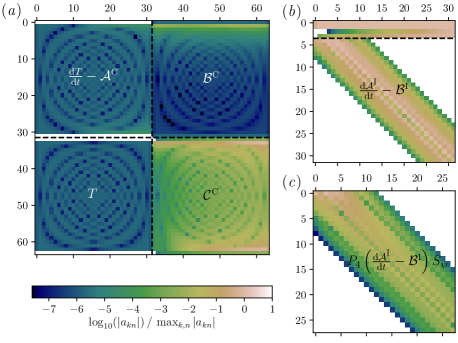
Figure 1: Representation of the coefficients of the left-hand-side matrices obtained for $m=4$ for a setup with $E=10^{-3}$, $Ra=3\times 10^{4}$ and $Pr=1$ and a CNAB2 time scheme with a fixed $\delta t=10^{-4}$. (a) corresponds to the collocation method (Eq. 16). $T$ corresponds to the matrix with the coefficients $T_{kn}=T_{n}(x_{k})$. (b) corresponds to the Chebyshev integration method with boundary conditions imposed as the first four tau lines (Eq. 25). (c) corresponds to Chebyshev integration method with boundary conditions enforced via a Galerkin formulation (Eq. 32). For the three panels, the matrix coefficients have been normalised by their maxima such that they share the same color axis. Zero entries are displayed in white.

3.2 Spectral equations using a Chebyshev integration method

To circumvent the limitations inherent in the collocation approach, several efficient Chebyshev spectral methods have been developed (e.g. Coutsias et al., 1996; Julien & Watson, 2009; Olver & Townsend, 2013). They all involve the solve of sparse matrices that are almost banded and can be inverted in $\mathcal{O}(p\,N_{r})$ operations, $p$ being the number of bands of the matrices. One approach, first introduced by Clenshaw (1957), consists of integrating $q$ times a set of $q$th-order ordinary differential equations (ODEs) in Chebyshev space (see also Fox & Parker, 1968; Phillips & A., 1990; Greengard, 1991). First limited to ODEs with constant coefficients, this method has been further extended by Coutsias et al. (1996) to ODEs with rational function coefficients. The comparison of several Chebyshev methods for fourth-order ODEs carried out by Muite (2010) showed the advantages of such a Chebyshev integration method both in terms of matrix condition number and computational cost in the limit of large $N_{r}$. This technique has been successfully applied to the problem of rotating convection in both Cartesian (Stellmach & Hansen, 2008) and spherical geometry (Marti et al., 2016).

3.2.1 Semi-discrete formulation

The Chebyshev integration methodology relies on the following indefinite integral identity (e.g. Canuto et al., 2006, Eq. 2.4.23)

$$\int T_{n}(x)\mathrm{d}x=\dfrac{1}{2}\left[\dfrac{T_{n+1}(x)}{n+1}-\dfrac{T_{n-1}(x)}{n-1}\right]~{}\text{for}~{}n>1,$$ (21)

which in its discrete form corresponds to the following sparse operator

$$\widehat{\mathcal{I}}_{kn}=-\dfrac{1}{2k}\delta_{k+1,n}+\dfrac{1}{2k}\delta_{k-1,n}~{}\text{for}~{}k>1,$$

where $\delta$ corresponds to the Kronecker symbol. Identities for multiple integration can then be easily derived by recursive applications of Eq. (21).

Because of the singularity of $\beta$, we first need to regularise the set of equation (4-8) to make it suitable for a Chebyshev integration method. We hence adopt the following different definition for the streamfunction $\varPsi$

$$u_{s}=\dfrac{1}{s}\dfrac{\partial[\zeta(s)\varPsi]}{\partial\phi};\quad u_{\phi}=\overline{u_{\phi}}-\dfrac{\partial[\zeta(s)\varPsi]}{\partial s}-\beta\zeta(s)\varPsi\,.$$

Using $\zeta(s)=h^{2}=s_{o}^{2}-s^{2}$ then yields

$$u_{s}=\dfrac{h^{2}}{s}\dfrac{\partial\varPsi}{\partial\phi};\quad u_{\phi}=\overline{u_{\phi}}-h^{2}\dfrac{\partial\varPsi}{\partial s}+3s\,\varPsi\,.$$ (22)

From these definitions, one derives the following expression for the axial vorticity $\omega$

$$\omega=\dfrac{1}{s}\dfrac{\partial(s\overline{u_{\phi}})}{\partial s}-\mathcal{L}_{I}\varPsi\,,$$ (23)

where the operator $\mathcal{L}_{I}$ is given by

$$\mathcal{L}_{I}\varPsi=\Delta\left(h^{2}\varPsi\right)-\dfrac{1}{s}\dfrac{\partial}{\partial s}\left(s^{2}\varPsi\right)\,.$$

The expansion of $\varPsi$ and $\vartheta$ in Fourier modes yields the following equation for the time evolution of $\varPsi$ for the non-axisymmetric Fourier modes

$$\left[\left(\dfrac{\partial}{\partial t}-\Delta\right)\mathcal{L}_{I}-\dfrac{2}{E}\mathrm{i}m\right]\varPsi_{m}=\dfrac{Ra}{Pr}\dfrac{\mathrm{i}m}{s_{o}}\vartheta_{m}+\mathcal{N}_{\omega m}-\mathcal{F}_{\epsilon}(E,\varPsi_{m})\,.$$

In the above equation, the classical Ekman pumping term (Eq. 6) has been replaced by the approximated form $\mathcal{F}_{\epsilon}$ defined by

$$\mathcal{F}_{\epsilon}=\Upsilon_{\epsilon}\left[\mathcal{L}_{I}+\dfrac{s}{2}\dfrac{\partial}{\partial s}-\left(\dfrac{3s^{2}}{2h_{\epsilon}^{2}}+m^{2}+\dfrac{5\mathrm{i}ms_{o}}{2h_{\epsilon}}\right)\right]\varPsi_{m}$$ (24)

where $h_{\epsilon}=[(s_{o}+\epsilon)^{2}-s^{2}]^{1/2}$ corresponds to half the height of a geostrophic cylinder that would intersect a sphere with a slightly larger radius $s_{o}+\epsilon$, with $\epsilon\ll 1$. $\Upsilon_{\epsilon}$ is defined accordingly by $\Upsilon_{\epsilon}=s_{o}^{1/2}/E^{1/2}/h_{\epsilon}^{3/2}$ . This implies that $\mathcal{F}_{\epsilon}$ corresponds to the exact Ekman pumping contribution that would occur in a spherical QG set-up with an outer radius $s_{o}+\epsilon$. In other words, the approximated Ekman pumping $\mathcal{F}_{\epsilon}$ tends to approach the exact contribution $\mathcal{F}$ in the limit of vanishing $\epsilon$. This approximation is required when using a Chebyshev integration method to avoid the outer boundary singularity of the exact Ekman pumping term and to get a good spectral representation of this quantity once transformed to Chebyshev space. The error introduced by this approximation will be further assessed in § 6.

In addition, the Ekman pumping term requires special care since it comprises non-rational function coefficients. In contrast to the collocation method where it can be treated implicitly without any additional cost, this term shall hence be treated as yet another non-linear term since its implicit treatment would yield a dense operator with the Chebyshev integration method (Hiegemann, 1997).

The equation for the time evolution of $\varPsi$ is regularised by a multiplication by $s^{4}$ and then integrated four times to yield

$$\int\!\!\!\!\int\!\!\!\!\int\!\!\!\!\int s^{4}\left[\left(\dfrac{\partial}{\partial t}-\Delta\right)\mathcal{L}_{I}-\dfrac{2}{E}\mathrm{i}m\right]\varPsi_{m}=\alpha r^{3}+\beta r^{2}+\gamma r+\delta$$ (25)

$$+\int\!\!\!\!\int\!\!\!\!\int\!\!\!\!\int s^{4}\left[\dfrac{Ra}{Pr}\dfrac{\mathrm{i}m}{s_{o}}\vartheta_{m}+\mathcal{N}_{\omega m}-\mathcal{F}_{\epsilon}(E,\varPsi_{m})\right]\,,$$

where $\alpha,\beta,\gamma$ and $\delta$ are constant of integration that will not be required once this equation has been supplemented by boundary conditions. At this stage, any single term that enters the above equation can be written as the product $x^{q}\partial^{p}f/\partial x^{p}$, where $p$ and $q$ are positive integers. Following Marti et al. (2016), this equation is then integrated by parts until no differential operator remains, such that each term has the following form

$$\sum_{p=0}^{4}\underbrace{\int\cdots\int}_{p\times}\left(\sum_{q}x^{q}f(x)\right)\mathrm{d}x^{p}\,.$$

After expanding $f(x)$ in Chebyshev polynomials using Eq. (14), the semi-discrete representation of Eq. (25) can be derived by multiple application of the recurrence relation (21). This yields

$$\sideset{}{{}^{\prime\prime}}{\sum}_{n=0}^{N_{c}-1}\left(\dfrac{\mathrm{d}}{\mathrm{d}t}\mathcal{A}^{I}_{mkn}-\mathcal{B}^{I}_{mkn}\right)\widehat{\varPsi}_{mn}(t)=$$ (26)

$$\sideset{}{{}^{\prime\prime}}{\sum}_{n=0}^{N_{c}-1}\mathcal{C}^{I}_{kn}\left[\dfrac{Ra}{Pr}\dfrac{\mathrm{i}m}{s_{o}}\widehat{\vartheta}_{mn}(t)+\widehat{\mathcal{N}}_{\omega mn}-\widehat{\mathcal{F}}_{\epsilon\,n}(E,\varPsi_{m})\right],$$

for $k>4$. $\mathcal{A}^{I}_{mkn}$, $\mathcal{B}^{I}_{mkn}$, and $\mathcal{C}^{I}_{kn}$ are the discrete representations of the following operators

$$\mathcal{A}^{I}_{m}=\int\!\!\!\!\int\!\!\!\!\int\!\!\!\!\int s^{4}\mathcal{L}_{I}; \mathcal{B}^{I}_{m}=\int\!\!\!\!\int\!\!\!\!\int\!\!\!\!\int s^{4}\left(\Delta\mathcal{L}_{I}+\dfrac{2}{E}\mathrm{i}m\right);$$

$$\mathcal{C}^{I}=\int\!\!\!\!\int\!\!\!\!\int\!\!\!\!\int s^{4}$$

The internal matrix elements are determined using the freely available python package developed by Marti et al. (2016) that allows the symbolic computation of those operators. Excluding boundary conditions, $\mathcal{A}^{I}_{m}$, $\mathcal{B}^{I}_{m}$ and $\mathcal{C}^{I}$ correspond to band matrices with $p_{u}$ super-diagonals and $p_{\ell}$ sub-diagonals that have a bandwidth defined by

$$q=p_{\ell}+p_{u}+1\,.$$

The bandwidth of $\mathcal{A}^{I}_{m}$, $\mathcal{B}^{I}_{m}$, and $\mathcal{C}^{I}$ is 17, 13 and 17, respectively.

We proceed the same way to establish the equations for the axisymmetric zonal flow component and for the temperature perturbation. Eq. (7) and Eq. (8) are multiplied by $s^{2}$ and integrated twice to yield

$$\sideset{}{{}^{\prime\prime}}{\sum}_{n=0}^{N_{c}-1}\left(\dfrac{\mathrm{d}}{\mathrm{d}t}\mathcal{D}^{I}_{kn}-\mathcal{E}^{I}_{kn}\right)\widehat{u_{\phi}}_{0n}(t)=$$ (27)

$$-\sideset{}{{}^{\prime\prime}}{\sum}_{n=0}^{N_{c}-1}\mathcal{D}^{I}_{kn}\left[\widehat{\mathcal{N}}_{u_{\phi}mn}+\widehat{\Upsilon_{\epsilon}{u_{\phi}}_{0}}_{n}\right],$$

for the axisymmetric zonal flow component and

$$\sideset{}{{}^{\prime\prime}}{\sum}_{n=0}^{N_{c}-1}\left(\dfrac{\mathrm{d}}{\mathrm{d}t}\mathcal{D}^{I}_{kn}-\dfrac{1}{Pr}\mathcal{F}^{I}_{kmn}\right)\widehat{\vartheta}_{mn}(t)=$$ (28)

$$-\sideset{}{{}^{\prime\prime}}{\sum}_{n=0}^{N_{c}-1}\mathcal{D}_{kn}\left[\mathrm{i}m\widehat{\left(\dfrac{h^{2}}{s}\dfrac{\mathrm{d}T_{c}}{\mathrm{d}s}\varPsi_{m}\right)}_{n}+\widehat{\mathcal{N}}_{\vartheta mn}\right],$$

for the temperature. Both equations are only valid for $k>2$. $\mathcal{D}^{I}_{kn}$, $\mathcal{E}^{I}_{kn}$ and $\mathcal{F}^{I}_{mkn}$ are the discrete representation of the following operators

$$\mathcal{D}^{I}=\int\!\!\!\!\int s^{2};\ \mathcal{E}^{I}=s^{2}-3\int s;\ \mathcal{F}^{I}_{m}=\int\!\!\!\!\int s^{2}\Delta\,.$$

The bandwidth of $\mathcal{D}^{I}$, $\mathcal{E}^{I}$ and $\mathcal{F}^{I}_{m}$ is 9, 5 and 5, respectively. In contrast to the semi-discrete equations obtained with the collocation approach, the right-hand-sides of Eq. (26-28) now involve nonlinear terms that are in Chebyshev space. To avoid aliasing errors, the Chebyshev coefficients of nonlinear terms that have $n>2N_{r}/3$ are hence set to zero (Orszag, 1971).

3.2.2 Boundary conditions

At this stage, the system of equation (26-28) needs to be supplemented by boundary conditions. Given the definition of $\varPsi$, the rigid mechanical boundary conditions that require the cancellation of $u_{s}$ and $u_{\phi}$ at both boundaries are already ensured by the three following identities:

$$\varPsi(s=s_{i})=\dfrac{\partial\varPsi}{\partial s}(s=s_{i})=0,\quad\varPsi(s=s_{o})=0\,.$$ (29)

An extra boundary condition on $\varPsi$ is thus required. Following Bardsley (2018), we make the ansatz

$$\varPsi\sim(s_{o}^{2}-s^{2})^{n}\ \text{when}\ s\rightarrow s_{o}\,.$$

This yields the following expression for the viscous term

$$\Delta\mathcal{L}_{I}\varPsi=\dfrac{1}{s^{4}}(s_{o}^{2}-s^{2})^{n-3}\left[8n\,s_{o}^{8}\,(-2n^{3}+3n^{2}+5n-6)\right]\,,$$

when $s\rightarrow s_{o}$. A finite solution requires either $n>3$ or the cancellation of the poynomial on $n$, which has four roots $(-3/2,0,1,2)$. $n=-3/2$ is not allowed and $n=0$ is redundant with the cancellation of $\varPsi$ at $s=s_{o}$. Hence the first possible solution is $n=1$ which yields

$$\varPsi\sim s^{2}-s_{o}^{2}\ \text{when}\ s\rightarrow s_{o}\,.$$

This corresponds to the following additional boundary condition

$$\dfrac{\partial^{3}\varPsi}{\partial s^{3}}=0\ \text{for}\ s=s_{o}\,.$$ (30)

When using the Chebyshev integration method, the boundary conditions can be either enforced via the tau-Lanczos method or by setting up an adapted Galerkin basis function (Canuto et al., 2006; Boyd, 2001). In the tau-Lanczos formulation, the top rows of the matrices are used to enforce the boundary conditions, which are actually identical to the ones used in the collocation method (Eqs. 19-20). The fourth condition on $\varPsi$ given in Eq. (30) corresponds to the following last tau line (see Julien & Watson, 2009)

$$\sideset{}{{}^{\prime\prime}}{\sum}_{n=0}^{N_{c}-1}n^{2}(n^{2}-1)(n^{2}-4)\,\widehat{\varPsi}_{n}=0\,.$$ (31)

Figure 1b shows the structure of the matrix that enters the left-hand-side of Eq. (26) when the boundary conditions are enforced using a tau-Lanczos formulation. The two first rows of the matrix correspond to the Dirichlet boundary conditions (Eqs. 19 and 29), the third one to the above equation and the fourth one to the Neumann boundary condition (Eqs. 20 and 29). Below those four full lines the matrix has a banded structure with 8 sub- and super-diagonals. This corresponds to a so-called bordered matrix wich can be inverted in $\mathcal{O}(17\,N_{r})$ operations as long as the number of full rows is small compared to the problem size (e.g. Boyd, 2001). Appendix A gives the details of the matrix inversion procedure as implemented in pizza.

We proceed the same way for the boundary conditions on the axisymmetric zonal flow and on the temperature. In those cases the Dirichlet boundary conditions (19) are imposed as the two first tau lines of the matrix, while the banded structure below is given by (27) and (28), respectively.

Alternatively, the boundary conditions can be imposed by introducing a suitable Galerkin basis. The underlying idea is to define basis functions that satisfy the boundary conditions such that the solutions expressed on this set of functions will also directly fulfill the boundary conditions. The Galerkin basis of functions $\phi_{m}$ is usually defined as a linear combination of a small number $n_{c}$ of Chebyshev polynomials

$$\phi_{n}(x)=\sum_{i=0}^{n_{c}-1}\gamma_{i}^{n}T_{n+i}(x)\,.$$

We first construct the Galerkin basis for the four boundary conditions on $\varPsi$ (Eqs. 29 and 30). Following Julien & Watson (2009), the tau conditions (19,  20, 31) are used to establish a related Galerkin set. Appendix B gives the details of the calculation of the $\gamma_{i}^{n}$ coefficients for $0\leq i\leq 4$. $\varPsi$ is then decomposed on the Galerkin basis as follows

$$\varPsi(s)=\sum_{n=0}^{N_{r}-5}\widetilde{\varPsi}_{n}\phi_{n}(x)\,,$$

where the tilda notation denotes the Galerkin coefficients. The Galerkin coefficients $\widetilde{\varPsi}$ relate to the Chebyshev coefficients $\widehat{\varPsi}$ via

$$\widehat{\varPsi}=S_{\varPsi}\,\widetilde{\varPsi},$$

where $S_{\varPsi}$ is the stencil matrix that contains the coefficients $\gamma_{i}$. For the Galerkin basis employed for the equation on $\varPsi$, $S_{\varPsi}$ is a band matrix with four sub-diagonals. The Galerkin formulation of Eq. (26) can be hence written in its matrix form as

$$P_{4}\left(\dfrac{\mathrm{d}\mathcal{A}^{I}_{m}}{\mathrm{d}t}-\mathcal{B}^{I}_{m}\right)S_{\varPsi}\,\widetilde{\varPsi}_{m}=P_{4}C^{I}\left[\dfrac{Ra}{Pr}\dfrac{\mathrm{i}m}{s_{o}}\widehat{\vartheta}_{m}+\widehat{\mathcal{N}}_{\omega m}-\widehat{\mathcal{F}}_{\epsilon}\right],$$ (32)

where $P_{4}$ is an operator that removes the top four rows of the matrices, which correspond to the number of boundary conditions (Julien & Watson, 2009). Figure 1c shows the structure of the matrix that enters the left-hand-side of Eq. (32). Compared to the bordered matrix obtained when using the tau method, the matrix has now a pure banded structure with an increased bandwidth with 8 sub- and 12 super-diagonals. Those matrices could be solved using standard band matrix solvers. In pizza, the LU decomposition is handled by the LAPACK routine dgbtrf or its complex arithmetic counterpart zgbtrf in $\mathcal{O}(q^{2}\,N_{r})$ operations per Fourier mode $m$. dgbtrs (or zgbtrs) routines are then employed for the matrix solve in $\mathcal{O}(q\,N_{r})$ operations per Fourier mode $m$.

We proceed the same way for the zonal velocity and the temperature equations by defining a Galerkin basis that ensures Dirichlet boundary conditions at both boundaries. Several different Galerkin basis sets that satisfy this type of boundary conditions have been frequently used in the context of modelling rotating convection (e.g. Pino et al., 2000; Stellmach & Hansen, 2008). Following Julien & Watson (2009), we decide here to adopt the following set

$$\phi_{n}(x)=T_{n+2}(x)-T_{n}(x),\quad\text{for}\quad n<N_{r}-3\,.$$ (33)

In matrix form, the Galerkin formulations of equations (27) and (28) yield

$$P_{2}\left(\dfrac{\mathrm{d}\mathcal{D}^{I}}{\mathrm{d}t}-\mathcal{E}^{I}\right)S_{\text{D}}\,\widetilde{u_{\phi}}_{0}=\\ -P_{2}\mathcal{D}^{I}\left[\widehat{\mathcal{N}}_{u_{\phi}m}+\widehat{\Upsilon_{\epsilon}{u_{\phi}}_{0}}\right],$$ (34)

for the axisymmetric zonal flow component and

$$P_{2}\left(\dfrac{\mathrm{d}D^{I}}{\mathrm{d}t}-\dfrac{\mathcal{F}^{I}_{m}}{Pr}\right)S_{\text{D}}\,\widetilde{\vartheta}_{m}=-P_{2}\mathcal{D}^{I}\left[\mathrm{i}m\widehat{\left(\dfrac{h^{2}}{s}\dfrac{\mathrm{d}T_{c}}{\mathrm{d}s}\varPsi_{m}\right)}+\widehat{\mathcal{N}}_{\vartheta m}\right],$$ (35)

for the temperature, where $S_{\text{D}}$ is the stencil matrix (33) and $P_{2}$ is an operator that removes the top two rows.

We note that different type of boundary conditions, such as stress-free and/or fixed flux thermal boundary conditions, would necessitate the derivation of dedicated Galerkin bases following a procedure similar to the one discussed in the appendix B.

Previous analysis by Julien & Watson (2009) showed that the Galerkin approach usually yield matrices with a better condition number than the bordered matrices obtained when using the tau-Lanczos method. This is particularly critical when 2-D or 3-D Chebyshev domains are considered but remains acceptable for 1-D problem as considered here (see Table 1 in Julien & Watson, 2009). The Galerkin approach should hence be privileged as long as homogeneous boundary conditions are enforced, while inhomogeneous boundary conditions for which a Galerkin description becomes cumbersome are easier to handle with a tau-Lanczos formulation.

4 Temporal discretisation

Table 1: Time schemes implemented in pizza. The fifth ($\mathcal{I}$) and the sixth columns ($\mathcal{E}$) correspond to the number of implicit and explicit terms computed for one time step, respectively. The seventh column (Storage) is the number of state vectors that need to be stored to time-advance one physical quantity. The eighth column (Cost) corresponds to the elapsed wall time for one iteration normalised by the cost for one iteration of CNAB2. The last column contains the maximum CFL $\alpha$ obtained for a case with $E=10^{-7}$, $Ra=2\times 10^{11}$, $Pr=1$ and $\epsilon=10^{-3}$ which has been computed using the Chebyshev integration and Galerkin methods with $(N_{r},N_{c},N_{m})=(1025,682,1280)$. The asterisks corresponds to the models which have been run with an explicit treatment of the buoyancy term.

Name	Family	Reference	Order	$\mathcal{I}$	$\mathcal{E}$	Storage	Cost	$\alpha$
SBDF4	Multi-step	Wang & Ruuth (2008), Eq. (2.15)	4	1	1	8	1.01	0.19
SBDF3	Multi-step	Peyret (2002), Eq. (4.83)	3	1	1	6	0.97	0.23
SBDF2	Multi-step	Peyret (2002), Eq. (4.82)	2	1	1	4	0.96	0.21
CNAB2	Multi-step	Glatzmaier (1984), Eq. (5b)	2	1	1	4	1	0.25
BPR353	SDIRK	Boscarino et al. (2013), § 8.3	3	5	3	9	3.24	$0.78^{*}$
ARS443	SDIRK	Ascher et al. (1997), § 2.8	3	4	3	9	3.66	$0.71^{*}$
ARS222	SDIRK	Ascher et al. (1997), § 2.6	2	2	2	5	1.81	$0.45^{*}$
LZ232	SDIRK	Liu & Zou (2006), § 6	2	2	2	6	1.86	$0.42^{*}$

The equations discretised in space can be written as a general ordinary differential equation in time where the right-hand-side is split in two contributions

$$\dfrac{\mathrm{d}y}{\mathrm{d}t}=\mathcal{E}(y,t)+\mathcal{I}(y,t),\quad y(t_{0})=y_{0},$$ (36)

where $\mathcal{I}(y,t)$ corresponds to the linear terms, while $\mathcal{E}(y,t)$ corresponds to the nonlinear advective terms. Temporal stability constraints coming from the linear terms that enter Eqs. (5-8) is usually more stringent that the one coming from the nonlinear terms. Except for weakly nonlinear calculations, this precludes the usage of purely explicit time schemes such as the popular fourth order Runge-Kutta (e.g. Grooms & Julien, 2011). Although they offer an enhanced stability, purely implicit schemes are extremely costly since they involve the coupling of all Fourier modes due to the implicit treatment of the nonlinear terms. The potential gain in time step size is hence cancelled by the numerical cost associated with the solve of large matrices. In the following, we hence only consider implicit-explicit schemes (hereafter IMEX) to solve Eq. (36) and to produce the numerical approximation $y_{n}\simeq y(t_{n})$. We first consider the general $k$-step IMEX linear multistep scheme

$$y_{n+1}=\sum_{j=1}^{k}a_{j}y_{n+1-j}+\delta t\left(\sum_{j=1}^{k}b^{\mathcal{E}}_{j}\mathcal{E}_{n+1-j}+\sum_{j=0}^{k}b^{\mathcal{I}}_{j}\mathcal{I}_{n+1-j}\right),$$ (37)

where $\mathcal{E}_{n+1-j}=\mathcal{E}(y_{n+1-j},t_{n+1-j})$ and $\mathcal{I}_{n+1-j}=\mathcal{I}(y_{n+1-j},t_{n+1-j})$. The vectors $\textstyle a$, $\mathchoice{\mbox{\boldmath$\displaystyle b$}}{\mbox{\boldmath$\textstyle b$}}{\mbox{\boldmath$\scriptstyle b$}}{\mbox{\boldmath$\scriptscriptstyle b$}}^{\mathcal{E}}$ and $\mathchoice{\mbox{\boldmath$\displaystyle b$}}{\mbox{\boldmath$\textstyle b$}}{\mbox{\boldmath$\scriptstyle b$}}{\mbox{\boldmath$\scriptscriptstyle b$}}^{\mathcal{I}}$ correspond to the weighting factors of the IMEX multistep scheme. For instance, the commonly-used second-order scheme assembled from the combination of a Crank-Nicolson for the implicit terms and a second-order Adams-Bashforth for the explicit terms (hereafter CNAB2) corresponds to the following vectors $\mathchoice{\mbox{\boldmath$\displaystyle a$}}{\mbox{\boldmath$\textstyle a$}}{\mbox{\boldmath$\scriptstyle a$}}{\mbox{\boldmath$\scriptscriptstyle a$}}=(1,0)$, $\mathchoice{\mbox{\boldmath$\displaystyle b$}}{\mbox{\boldmath$\textstyle b$}}{\mbox{\boldmath$\scriptstyle b$}}{\mbox{\boldmath$\scriptscriptstyle b$}}^{\mathcal{I}}=(1/2,1/2)$ and $\mathchoice{\mbox{\boldmath$\displaystyle b$}}{\mbox{\boldmath$\textstyle b$}}{\mbox{\boldmath$\scriptstyle b$}}{\mbox{\boldmath$\scriptscriptstyle b$}}^{\mathcal{E}}=(3/2,-1/2)$ for a constant $\delta t$. In practice, Eq. (37) is rearranged as follows

$$(I-b_{0}^{\mathcal{I}}\delta t\,\mathcal{I})\,y_{n+1}= \sum_{j=1}^{k}a_{j}y_{n+1-j}$$ (38)

$$+\delta t\sum_{j=1}^{k}\left(b_{j}^{\mathcal{E}}\mathcal{E}_{n+1-j}+b_{j}^{\mathcal{I}}\mathcal{I}_{n+1-j}\right)\,,$$

where $I$ is the identity matrix. In addition to CNAB2, pizza supports several semi-implicit backward differentiation schemes of second, third and fourth order that are known to have good stability properties (heareafter SBDF2, SBDF3 and SBDF4, see Ascher et al., 1995; Garcia et al., 2010). The interested reader is referred to the work by Wang & Ruuth (2008) for the derivation of the vectors $\textstyle a$, $\mathchoice{\mbox{\boldmath$\displaystyle b$}}{\mbox{\boldmath$\textstyle b$}}{\mbox{\boldmath$\scriptstyle b$}}{\mbox{\boldmath$\scriptscriptstyle b$}}^{\mathcal{I}}$ and $\mathchoice{\mbox{\boldmath$\displaystyle b$}}{\mbox{\boldmath$\textstyle b$}}{\mbox{\boldmath$\scriptstyle b$}}{\mbox{\boldmath$\scriptscriptstyle b$}}^{\mathcal{E}}$ when the time step size is variable. Table 1 summarises the main properties of the multistep schemes implemented in pizza.

Multistep schemes suffer from several possible limitations: (i) when the order is larger than two, they are not self-starting and hence require to be initiated with another lower-order starting scheme; (ii) limitations of the time step size to maintain stability is more severe for higher-order schemes (e.g. Ascher et al., 1995; Carpenter et al., 2005). In contrast, the multi-stage Runge-Kutta schemes are self-starting and frequently show a stability region that grows with the order of the scheme. To examine their efficiency in the context of spherical QG convection, we have also implemented in pizza several Additive Runge Kutta schemes. For this type of IMEX, we restrict ourself to the so-called Diagonally Implicit Runge Kutta schemes (hereafter DIRK) for which each sub-stage can be solved sequentially. For such schemes, the equation (36) is time-advanced from $t_{n}$ to $t_{n+1}$ by solving $\nu$ sub-stages

$$\left(I-a_{ii}^{\mathcal{I}}\delta t\,\mathcal{I}\right)y_{i}=y_{n}+\delta t\sum_{j=1}^{i-1}\left(a_{i,j}^{\mathcal{E}}\mathcal{E}_{j}+a_{i,j}^{\mathcal{I}}\mathcal{I}_{j}\right),\ 1\leq i\leq\nu,$$ (39)

where $y_{i}$ is the intermediate solution at the stage $i$. Finally the evaluation of

$$y_{n+1}=y_{n}+\delta t\sum_{j=1}^{\nu}\left(b_{j}^{\mathcal{E}}\mathcal{E}_{j}+b_{j}^{\mathcal{I}}\mathcal{I}_{j}\right).$$

allows the determination of $y_{n+1}$. A DIRK scheme with $\nu$ stages can be represented in terms of the following so-called Butcher tables

$$\begin{array}[]{c|c}\mathchoice{\mbox{\boldmath$\displaystyle c$}}{\mbox{\boldmath$\textstyle c$}}{\mbox{\boldmath$\scriptstyle c$}}{\mbox{\boldmath$\scriptscriptstyle c$}}^{\mathcal{I}}&\mathbf{A}^{\mathcal{I}}\\ \hline\cr&\mathchoice{\mbox{\boldmath$\displaystyle b$}}{\mbox{\boldmath$\textstyle b$}}{\mbox{\boldmath$\scriptstyle b$}}{\mbox{\boldmath$\scriptscriptstyle b$}}^{\mathcal{I}}\end{array}=\begin{array}[]{c|ccccc}c_{1}^{\mathcal{I}}&a_{11}^{\mathcal{I}}\\ c_{2}^{\mathcal{I}}&a_{21}^{\mathcal{I}}&a_{22}^{\mathcal{I}}\\ \vdots&\vdots&\vdots&\ddots\\ c_{\nu}^{\mathcal{I}}&a_{\nu 1}^{\mathcal{I}}&a_{\nu 2}^{\mathcal{I}}&\cdots&a_{\nu\nu}^{\mathcal{I}}\\ \hline\cr&b_{1}^{\mathcal{I}}&b_{2}^{\mathcal{I}}&\cdots&b_{\nu}^{\mathcal{I}}\end{array}\,,$$

for the implicit terms, and

$$\begin{array}[]{c|c}\mathchoice{\mbox{\boldmath$\displaystyle c$}}{\mbox{\boldmath$\textstyle c$}}{\mbox{\boldmath$\scriptstyle c$}}{\mbox{\boldmath$\scriptscriptstyle c$}}^{\mathcal{E}}&\mathbf{A}^{\mathcal{E}}\\ \hline\cr&\mathchoice{\mbox{\boldmath$\displaystyle b$}}{\mbox{\boldmath$\textstyle b$}}{\mbox{\boldmath$\scriptstyle b$}}{\mbox{\boldmath$\scriptscriptstyle b$}}^{\mathcal{E}}\end{array}=\begin{array}[]{c|ccccc}0&0\\ c_{2}^{\mathcal{E}}&a_{21}^{\mathcal{E}}&0\\ \vdots&\vdots&\vdots&\ddots\\ c_{\nu}^{\mathcal{E}}&a_{\nu 1}^{\mathcal{E}}&a_{\nu 2}^{\mathcal{E}}&\cdots&0\\ \hline\cr&b_{1}^{\mathcal{E}}&b_{2}^{\mathcal{E}}&\cdots&b_{\nu}^{\mathcal{E}}\end{array}\,,$$

for the explicit terms, where zero values above the diagonal have been omitted. In the following, we only consider the stiffly accurate DIRK schemes for which the outcome of the last stage gives the end-result, without needing any assembly stage (Ascher et al., 1997). This corresponds to $b_{j}^{\mathcal{I}}=a_{\nu j}^{\mathcal{I}}$ and $b_{j}^{\mathcal{E}}=a_{\nu j}^{\mathcal{E}}$ for $1<j<\nu$. In addition, to minimise the memory storage which is particularly critical in the Chebyshev collocation approach, only the DIRK schemes that involve one single matrix storage in the implicit solve are retained, i.e. $a_{ii}^{\mathcal{I}}$ is independent of $i$. The latter restriction corresponds to the so-called SDIRK (Singly Diagonally Implicit Runge–Kutta) schemes. In the following we discuss the convergence and the stability properties of two second order –ARS222 from Ascher et al. (1997) and LZ232 from Liu & Zou (2006)–; and two third order SDIRK schemes –ARS443 from Ascher et al. (1997) and BPR353 from Boscarino et al. (2013)–.

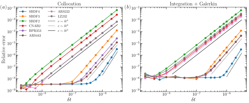
Figure 2: Relative error as a function of the time step size $\delta t$ for several multistep and SDIRK time schemes when using Chebyshev collocation (left panel) and Chebyshev integration method with boundary conditions enforced by a Galerkin approach (right panel). For comparison, the expected convergence orders have been denoted by black lines. Those convergence analyses have been carried out at the saturated stage of a numerical setup with $E=3\times 10^{-6}$, $Ra=10^{7}$ and $Pr=0.025$. Spatial resolution corresponds to ($N_{r},N_{c},N_{m}=193,193,128$) for the collocation method and ($N_{r},N_{c},N_{m}=193,128,128$) for the integration method. $\epsilon=3\times 10^{-3}$ has been assumed for the Chebyshev integration method.

The nonlinear advection terms that enter Eqs. (4-7) are treated explicitly, while the dissipation terms and the vortex streching term in Eq. (5) are treated implicitly. As long as the fluid domain is entirely convecting, the buoyancy term that enters the vorticity equation (5) can either be treated explicitly or implicitly without a notable change of the stability properties of the IMEX (e.g. Stellmach & Hansen, 2008). We can expect more significant differences when some regions of the fluid are stably stratified. An implicit treatment of the buoyancy term only implies that the temperature equation (8) shall be first time-advanced to produce $\vartheta(t_{n+1})$ before time-advancing the vorticity and streamfunction (e.g. Glatzmaier, 1984). The treatment of the Ekman pumping terms depends on the spatial discretisation strategy: while this can be treated implicitly without additional cost in the collocation method, this term has to be treated explicitly when using the Chebyshev integration method.

For an illustrative purpose, we give here the time-stepping equation for $\widehat{\varPsi}_{m}$ when the Chebyshev integration method (Eq. 26) is used in conjunction with an SDIRK time scheme (Eq. 39)

$$\left(\mathcal{A}^{I}_{m}-a_{ii}^{\mathcal{I}}\delta t\,\mathcal{B}^{I}_{m}\right)\widehat{\varPsi}_{m}(t_{i})=\mathcal{A}^{I}_{m}\widehat{\varPsi}_{m}(t_{n})+\delta t\sum_{j=1}^{i-1}a_{i,j}^{\mathcal{I}}\,\mathcal{B}^{I}_{m}\widehat{\varPsi}_{m}(t_{j})$$

$$+\delta t\sum_{j=1}^{i-1}a_{i,j}^{\mathcal{E}}\,\mathcal{C}^{I}\left[\dfrac{Ra}{Pr}\dfrac{\mathrm{i}m}{s_{o}}\widehat{\vartheta}_{m}(t_{j})+\widehat{\mathcal{N}}_{\omega m}(t_{j})-\widehat{\mathcal{F}}_{\epsilon}(t_{j})\right],$$

where the buoyancy term has been treated explicitly and $1\leq i\leq\nu$. This equation needs to be solved $\nu$ times per time step and the outcome of the final stage produces the time-advanced quantity $\widehat{\varPsi}_{m}(t_{n+1})$ for the azimuthal wavenumber $m$. A summary of the main properties of the SDIRK schemes implemented in pizza is also given in Table 1.

Both families of time integrators (38) and (39) have a very similar structure and can hence be implemented using a shared framework, provided the programming language supports object-oriented implementation (Vos et al., 2011). In pizza we rely on the object-oriented features provided by the Fortran 2003 norm to implement an abstract framework that allows easy switching between different schemes while minimising the number of code lines.

The different time steppers have been validated by running convergence tests. To do so, we consider a physical test problem with $E=3\times 10^{-6}$, $Ra=10^{7}$, $Pr=0.025$ and initiate the numerical experiment with a random temperature perturbation. We then run the numerical model using an SBDF4 time stepper until a statistically steady-state has been reached. This final state serves as the starting conditions of a suite of numerical simulations that use different fixed time step size $\delta t$ between $10^{-9}$ and $3\times 10^{-6}$ over a fixed physical timespan $t=1.2\times 10^{-3}$. Following Grooms & Julien (2011), the error associated with the time stepper is defined as the sum of the relative errors on $\vartheta$, $u_{s}$ and $u_{\phi}$, where the relative error for one physical quantity $f$ is expressed by

$$e_{\text{rel}}(f)=\left[\dfrac{\left\langle(f-f_{\text{ref}})^{2}\right\rangle}{\left\langle f_{\text{ref}}^{2}\right\rangle}\right]^{1/2}\,.$$

In the above equation, the angular brackets correspond to an integration over the annulus

$$\langle f\rangle=\int_{0}^{2\pi}\int_{s_{i}}^{s_{o}}f(s,\phi)\,s\,\mathrm{d}s\,\mathrm{d}\phi\,.$$

The fourth-order SBDF4 time stepper with the smallest time step size $\delta t=10^{-9}$ has been used to define the reference solution $f_{\text{ref}}$. Figure 2 shows the error as a function of $\delta t$ for the time schemes given in Table 1 for both the collocation method (left panel) and the Chebyshev integration method with a Galerkin approach to enforce the boundary conditions (right panel). All schemes converge with their expected theoretical order until a plateau is reached around $3\times 10^{-9}$ for the Chebyshev collocation and $10^{-8}$ for the Chebyshev integration method. This can be attributed to the propagation of rounding errors that occur in the spectral transforms and in the calculation of the radial derivatives (Sánchez et al., 2004). In other words, at this level of $\delta t$ the error becomes dominated by the spatial discretisation errors. For a given order, SDIRK schemes are found to be more accurate than their multistep counterparts for the majority of the cases.

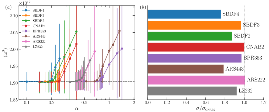
Figure 3: (a) Time-averaged total enstrophy $\langle\omega^{2}\rangle$ as a function of the CFL coefficient $\alpha$ for the time schemes given in Table 1. The error bars correspond to one standard deviation and the horizontal dashed line corresponds to the time-averaged enstrophy of a numerical model computed with the SBDF4 time scheme with $\alpha=0.05$. (b) Efficiency $\sigma$ of the time schemes normalised by the efficiency of CNAB2. The vertical dotted line corresponds to a value of one. This efficiency analysis has been carried out at the saturated stage of a numerical model with $E=10^{-7}$, $Pr=1$, $Ra=2\times 10^{11}$. This model was computed using the Chebyshev integration and a Galerkin method with a spatial resolution of ($N_{r},N_{c},N_{m}=1025,682,1280$) and $\epsilon=10^{-3}$.

This time scheme validation has been carried out with fixed time step sizes on a physical test case that is close to the onset of convection. To examine the efficiency of the different time schemes to model quasi-geostrophic turbulent convection, we also perform a stability analysis on a more turbulent setup. Indeed a precision of a fraction of a percent is usually sufficient when considering parameter studies of turbulent rotating convection (e.g. Gastine et al., 2016). Hence, the determination of the largest time step size $\delta t$ is of practical interest to assess the efficiency of a given time scheme. To do so, we consider a problem with $E=10^{-7}$, $Ra=2\times 10^{11}$ and $Pr=1$, which is approximately 60 times supercritical. We first time-advance the solution until the nonlinear saturation has been reached using a CNAB2 time scheme. We then use the final state of this computation as the starting conditions of several numerical simulations that use different time schemes. Those simulations are computed over $3\times 10^{-4}$ viscous time, which roughly corresponds to two turnover times. Since the advection terms are treated explicitly, the maximum eligible time step size must satisfy the following Courant criterion

$$\delta t\leq\alpha\min\left[\left(\max_{s,\phi}\dfrac{|u_{s}|}{\delta s}\right)^{-1},\left(\max_{s,\phi}\dfrac{|u_{\phi}|}{s\,\delta\phi}\right)^{-1}\right],$$ (40)

where $\delta s$ correspond to the local spacing of the Gauss-Lobatto grid and $\delta\phi=2\pi/3N_{m}$ to the constant spacing in the azimuthal direction. In the above equation, $\alpha$ corresponds to the Courant-Friedrichs-Lewy number (hereafter CFL). To determine the CFL number of each time scheme, we compute series of simulations with different values of $\alpha$ and let the code runs with the maximum allowed $\delta t$ that fulfills Eq. (40). This implies that $\delta t$ will change at each iteration and hence that the matrices will be rebuilt at each time step. Since LU factorisation is very demanding when using Chebyshev collocation ($\mathcal{O}(N_{r}^{3})$ operations), we restrict the stability analysis to the sparse Chebyshev integration method with a Galerkin approach to enforce the boundary conditions. We use the time evolution of the total enstrophy $\langle\omega^{2}\rangle$ as a diagnostic to estimate the maximum CFL number $\alpha$. Because of the clustering of the Gauss-Lobatto grid points, the time step size limitation usually occurs in the vicinity of the boundaries. Since $\langle\omega^{2}\rangle$ reaches its maximum value in the viscous boundary layers, any violation of Eq. (40) yields spurious spikes in the time evolution of the total enstrophy, well before the code actually crashes. For comparison, we define a reference solution that has been run with an SBDF4 time scheme with the smallest value of $\alpha=0.05$.

Figure 3a shows the time-averaged and the standard deviation of $\langle\omega^{2}\rangle$ as a function of $\alpha$ for the time schemes given in Table 1. The curves are comprised of two parts: one horizontal part where the time-averaged total enstrophy remains in close agreement with the reference case and the other featuring a rapid increase of both the time-averaged and the standard deviation of $\langle\omega^{2}\rangle$. We hence define the largest acceptable $\alpha$ for a given time scheme as the value above which the time-averaged total enstrophy becomes more than 0.3% larger than the reference value. The rightmost column of Table 1 documents the obtained values. All multi-step schemes exhibit comparable CFL numbers with only a weak dependence on the theoretical order of the scheme. This is in agreement with the study by Carpenter et al. (2005) who report comparable time step limitations for several SBDF schemes when the problem becomes numerically stiff. In contrast, the SDIRK schemes allow significantly larger CFL numbers with third-order schemes being more stable than the second-order ones. We quantify the efficiency of a time scheme by the ratio

$$\sigma=\dfrac{\alpha}{\text{cost}}\,,$$ (41)

where the cost corresponds to the average wall time of one iteration without LU factorisation (see the before last column in Table 1). Figure 3b shows a comparison of the relative efficiency of the time schemes compared to CNAB2. Although the CFL numbers are larger for the SDIRK schemes, they actually have a similar efficiency to multistep schemes due to their higher numerical cost. CNAB2 and ARS222 are found to be the most efficient second-order schemes, while BPR353 and SBDF3 are the best third-order schemes. The CFL numbers derived here are however only indicative since the stability of the schemes is expected to depend on the stiffness of the physical problem (e.g. Ascher et al., 1997; Carpenter et al., 2005). It is yet unclear whether the SDIRK schemes considered here will be able to compete with the multistep methods in the limit of turbulent quasi-geostrophic convection. Addressing this question would necessitate a systematic survey of the limits of stability of the time schemes over a broad range of Reynolds and Rossby numbers.

5 Parallelisation strategy

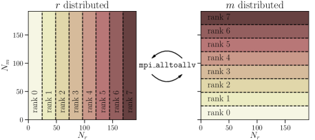
Figure 4: Domain decompositions used in pizza. The left panel corresponds to the MPI configuration where the radial levels are distributed among ranks and all $m$’s are in processor, while the right panel corresponds to the transposed configuration where the azimuthal wavenumbers are distributed and all radial level are in processor. The parallel transposition between those two representations is handled by mpi_alltoallv collective communications.

The implementation of the algorithm presented before in pizza has been designed to run efficiently on massively-parallel architectures. We rely on a message-passing communication framework based on the MPI (Message Passing Interface) standard. Several approaches have been considered to efficiently parallelise spectral transforms between physical and spectral space (e.g. Foster & Worley, 1997). Here we decide to resort to a transpose-based approach, such that all the spectral transforms are applied to data that are local to each processor. Whenever needed global transpositions of the data arrays are used to ensure that the dimension that needs to be transformed becomes local.

In pizza the data is distributed in two different configurations. In the first one, the radial level are distributed among MPI ranks while all azimuthal wavenumbers are local to each processor. This allows the computation of the 1D Fourier transforms (Eq. 12), the nonlinear terms in the physical space and the backward inverse transforms (Eq. 13). At this stage the data are rearranged in a second MPI configuration such that the wavenumbers $m$ are distributed, while all radial levels are now in processor. Since each processor can possibly have a different amount of data to be sent to other processors, this parallel transposition is handled by the MPI variant routine mpi_alltoallv that offers dedicated arguments to specify the amount of data to be sent and received from each partner. This configuration is used to time-advance the solution either via Chebyshev collocation (Eqs. 16-18) or via Chebyshev integration method (Eqs. 26-28). This implies the solve of linear problems and possibly DCTs (Eq. 14) to transform the data from Chebyshev to radial space. Figure 4 summarises the data distribution used in pizza.

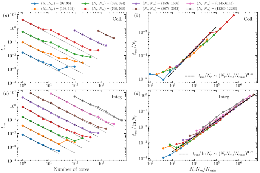
Figure 5: Left panels: wall time per iteration as a function of the number of MPI ranks (strong scaling performance) for several spatial resolutions. Right panels: wall time per iteration as a function of the local data volume per MPI task $N_{r}N_{m}/N_{\text{ranks}}$ (weal scaling performance). Panels (a) and (b) corresponds to the models that use the Chebyshev collocation method, while panels (c) and (d) correspond to the models where the Chebyshev integration is were used in conjunction with a Galerkin approach to enforce the boundary condition. In panels (a) and (c) the dotted black lines correspond to the ideal scalings. The linear fits displayed in panels (b) and (d) have been computed from the cases with $(N_{r},N_{m})=(1537,1536)$. All the simulations have been computed using the CNAB2 time scheme.

In the following, we examine the scalability performance of pizza using the occigen cluster. This cluster consists of more than 2000 computational nodes, each node being configured with two Intel 12 cores E5-2690V3 series processor with a clock frequency of 2.6 GHz. To build the executable, we make use of the Intel compiler version 17.0, Intel MPI version 5.1.3, Intel MKL version 17.0 for the linear solve and the matrix vector products and FFTW version 3.3.5 for Fourier and Chebyshev transforms. We first analyse the strong scaling performance of the code by running sequences of numerical simulations with several fixed problem size and an increasing number of MPI ranks. The left panels in Figure 5 show the wall time per iteration as a function of the number of cores for several problem sizes for both Chebyshev collocation and Chebyshev integration methods. The resolution $(N_{r},N_{m})$ range from $(97,96)$ to $(12289,12288)$. Because of the dense complex-type matrices of size $(2N_{r}\times 2N_{r})$ involved in the time advance of the coupled vorticity-streamfunction equation (16), we cannot use the collocation method for the largest problem sizes since it already requires more than 1 GB per rank when $N_{r}=1537$ and $N_{m}=1536$ with 128 MPI ranks. For the spatial resolutions that are sufficiently small to be computed on one single node, we observe an improved performance when the code is running on one single processor (i.e. up to 12 cores) with the Chebyshev collocation. This is not observed in the sparse cases and hence might be attributed to an internal speed-up of the dense matrix solver of the Intel MKL library. Apart from this performance shift, both methods show a scalability performance that improves with the problem size. While the efficiency of the strong scalings are quickly degraded for $N_{\text{ranks}}>N_{m}/8$ for small problem sizes, pizza shows a very good scalability up to $N_{\text{ranks}}=N_{m}/2$ for the largest problem sizes. The scalability performance of the collocation method is usually better than the Chebyshev integration method for a given problem size. This has to do with the larger amount of computational work spent in solving the dense matrices, which comparatively reduces the fraction of the wall time that corresponds to the MPI global transposes.

In complement to the strong scaling analyses, we also examine weak scaling performance tests. This consists of increasing the number of MPI ranks and the problem size accordingly, such that the amount of local data per rank stays constant. The spectral transforms implemented in pizza require $\mathcal{O}(N_{r}N_{m}\ln N_{m})$ operations for the FFTs (Eq. 12) and $\mathcal{O}(N_{m}N_{r}\ln N_{r})$ for the DCTs (Eq. 14). The solve of the linear problems involved in the time advance of the equations (4-8) grows like $\mathcal{O}(N_{m}N_{r}^{2})$ for the collocation method and only $\mathcal{O}(N_{m}N_{r})$ for the Chebyshev integration method. With the 1-D MPI domain decomposition discussed above, this implies that an increase of the spatial resolution while keeping a fixed amount of local data corresponds to an increase of the wall time that should scale with $\mathcal{O}(N_{r})$ for the collocation method and with $\mathcal{O}(\ln N_{r})$ for the Chebyshev integration method. The right panels of Fig 5 show the wall time per iteration normalised by those theoretical predictions as a function of the data volume per rank expressed by $N_{r}N_{m}/N_{\text{ranks}}$ for both Chebyshev methods. Using the simulations with a spatial resolution of $(N_{r},N_{m})=(1537,1536)$ we compute the following best fits between the normalised execution time and the local data volume for each radial discretisation scheme

$$\dfrac{t_{\text{run}}^{\text{coll.}}}{N_{r}} =2.2\times 10^{-8}\left(\dfrac{N_{r}N_{m}}{N_{\text{ranks}}}\right)^{0.98},$$ (42)

$$\ \dfrac{t_{\text{run}}^{\text{int.}}}{\ln N_{r}} =3.2\times 10^{-7}\left(\dfrac{N_{r}N_{m}}{N_{\text{ranks}}}\right)^{0.97},$$

where the run time is expressed in seconds. For both methods, the normalised wall time per iteration is nearly proportional to the data volume per rank, indicating a good agreement with the expected theoretical scalings. We can make use of those scalings to estimate the minimum theoretical execution time as a function of the problem size. Based on the results of the strong scaling analyses, we assume that pizza shows a good parallel efficiency up to $N_{\text{ranks}}=N_{m}/2$ when the collocation method is used and up to $N_{\text{ranks}}=N_{m}/4$ when a sparse Chebyshev formulation is employed. This yields

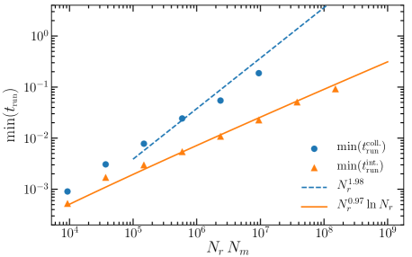
Figure 6: Minimum wall time per iteration as a function of the problem size $N_{r}N_{m}$. The lines correspond to the linear fits derived from the weak scaling tests (see Fig. 5b and d) for both radial discretisation strategies assuming $N_{\text{ranks}}=N_{m}/2$ for the collocation method and $N_{\text{ranks}}=N_{m}/4$ for the Chebyshev integration method combined with a Galerkin enforcement of boundary conditions. The symbols correspond to the minimum wall times obtained in the strong scaling analyses (Fig. 5a and c).

$$\min(t_{\text{run}}^{\text{coll.}}) =4.4\times 10^{-8}\,N_{r}^{1.98}\,,$$ (43)

$$\min(t_{\text{run}}^{\text{int.}}) =1.2\times 10^{-6}\,N_{r}^{0.97}\ln N_{r}\,.$$

Figure 6 shows a comparison between the actual minimum wall times for different spatial resolutions (see Fig. 5) and the above scalings. A good agreement is found for the sparse Chebyshev formulation and for the collocation method with $N_{r}N_{m}>10^{5}$. Since the computational time of FFTs and DCTs still represents a significant fraction of one time step for small problem sizes, this is not surprising that the scaling given in Eq. (43) is only approached for sufficiently large problem sizes when the collocation method is employed.

Adopting a Chebyshev integration formulation for the radial scheme provides a significant speed up over the collocation approach, with for instance a factor 10 gain when $N_{r}N_{m}\simeq 10^{7}$. Furthermore, while the collocation method becomes intractable for problem sizes with $N_{r}N_{m}>10^{7}$ because of its intrinsic large memory prerequisite, the sparse formulation can be employed for spatial resolution larger than $10^{4}\times 10^{4}$. Global synchronisation and file lock contention can become an issue when reaching this range of problem sizes. In pizza this is remedied by collective calls to MPI-IO write operations to handle the outputting of checkpoints and snapshots.

6 Code validation and examples

6.1 Weakly-nonlinear convection

In absence of a documented benchmark of spherical QG convection, we test the numerical implementation by first looking at the onset of convection. The underlying idea being to compare the results coming from a linear eigensolver with the results from pizza. The comparison of the different radial discretisation strategies is of particular interest to quantify the error introduced by the approximation of the Ekman pumping term involved in the sparse formulation (Eq. 24). To determine the onset of spherical QG convection, we linearise the system of equation (4-8) and seek for normal modes with

$$f(s,\phi,t)=\Re\left(\sum_{m=0}^{\infty}f_{m}(s)e^{\mathrm{i}m\phi+\lambda t}\right)\,,$$

where ${f_{m}}=(\psi_{m},\vartheta_{m})^{T}$ and $\lambda=\tau+\mathrm{i}\omega_{d}$, $\tau$ being the growth rate and $\omega_{d}$ the angular frequency. Since there is no coupling between the Fourier modes, we can seek for the solution $f_{m}$ of one individual azimuthal wavenumber. This forms the following generalised eigenvalue problem

$$\lambda\mathcal{L}_{\beta}\psi_{m} =\dfrac{Ra}{Pr}\dfrac{\mathrm{i}m}{s_{o}}\vartheta_{m}-\dfrac{2}{E}\dfrac{\mathrm{i}m}{s}\beta\psi_{m}-\mathcal{F}(E,\psi_{m})+\Delta(\mathcal{L}_{\beta}\psi_{m})\,,$$ (44)

$$\lambda\vartheta_{m} =\Delta\vartheta_{m}-\dfrac{\mathrm{i}m}{s}\dfrac{\mathrm{d}T_{c}}{\mathrm{d}s}\,\psi_{m}\,,$$

that is supplemented by the boundary conditions (11). We solve this generalised eigenvalue problem using the Linear Solver Builder package (hereafter LSB) developed by Valdettaro et al. (2007). The linear operators that enter Eq. (44) are discretised on the Gauss-Lobatto grid using a Chebyshev collocation method in real space (e.g. Canuto et al., 2006). The entire spectrum of complex eigenvalues $\lambda$ is first computed using the QZ algorithm (Moler & Stewart, 1973). One selected eigenvalue can then be used as a guess to accurately determine the closest eigenpair using the iterative Arnoldi-Chebyshev algorithm (e.g. Saad, 1992). As indicated in Table 2, the linear solver has been tested and validated against published values of critical Rayleigh numbers for spherical QG convection with or without Ekman pumping (Gillet et al., 2007).

Table 2: Onset of convection for $E=10^{-6}$, $Pr=0.025$ and $r_{i}/r_{o}=4/11$ from Gillet et al. (2007) and obtained with the Linear Solver Builder package. Note that the critical Rayleigh number $Ra_{c}$ from Gillet et al. (2007) have been normalised to match our definition.

	$Ra_{c}$	$m$	$\omega_{d}$
Without Ekman pumping
LSB	$1.3851\times 10^{7}$	$13$	$-1.3028\times 10^{4}$
Gillet et al. (2007)	$1.39\times 10^{7}$	$13$	$-1.300\times 10^{4}$
With Ekman pumping
LSB	$1.5231\times 10^{7}$	$14$	$-1.2705\times 10^{4}$
Gillet et al. (2007)	$1.53\times 10^{7}$	$14$	$-1.268\times 10^{4}$

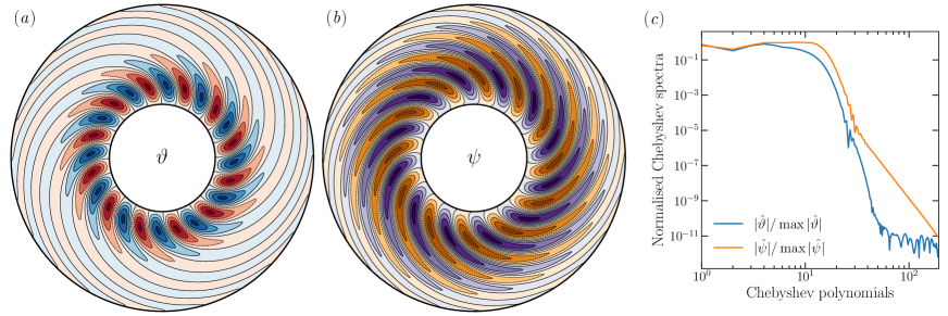
Figure 7: Eigenfunction of the first unstable mode for $E=3\times 10^{-6}$ and $Pr=0.025$. This mode has a critical Rayleigh number $Ra_{c}=9.55263\times 10^{6}$, a drift frequency $\omega_{d}=-9.42690\times 10^{3}$ and an azimuthal wavenumber $m=12$. (a) Temperature fluctuation $\vartheta$ in the equatorial plane. (b) Streamfunction $\psi$ in the equatorial plane. (c) Normalised Chebyshev spectra of the eigenfunction.

In the following we focus on weakly nonlinear QG convection with $E=3\times 10^{-6}$ and $Pr=0.025$ and a radius ratio $r_{i}/r_{o}=0.35$, a physical set up that is quite similar to the one considered by Gillet et al. (2007) for liquid Gallium. Figure 7 shows the critical eigenmode (with $\tau\simeq 0$) computed with LSB for these parameters. The onset of convection takes the form of a thermal Rossby wave that drifts in the retrograde direction with a critical azimuthal wavenumber $m=12$, a drifting frequency $\omega_{d}=-9.42690\times 10^{3}$ and a critical Rayleigh number $Ra_{c}=9.55263\times 10^{6}$. The numerical convergence of this calculation has been assessed by computing the Chebyshev spectra of the different eigenfunctions as illustrated on Fig. 7c.

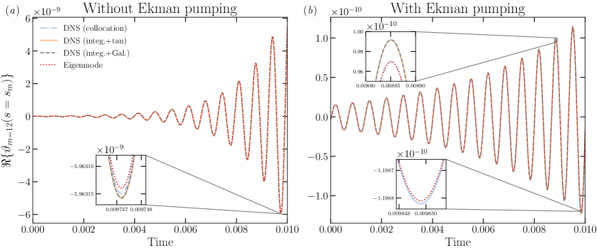
Figure 8: Real part of $\vartheta_{m=12}$ at mid-depth $s_{m}=0.5(s_{i}+s_{o})$ as a function of time without Ekman pumping (left panel) and with Ekman pumping (right panel) for a case with $E=3\times 10^{-6}$, $Ra=10^{7}$ and $Pr=0.025$. Zoomed-in insets highlight the differences between the eigenmode and the three spatial discretisation strategies implemented in pizza. The DNS have been time-advanced using the BPR353 time scheme with a fixed time step size $\delta t=10^{-7}$ to ensure that the error of the time scheme is negligible (see Fig. 2). The simulations have been initiated with the most unstable $m=12$ eigenmode calculated with LSB. Both sparse Chebyshev formulations assume $\epsilon=3\times 10^{-3}$ for the cases with Ekman pumping.

To validate the numerical implementation, the growth rate and the drift frequency obtained with pizza are compared to the eigenvalues derived with LSB. This requires a finite growth rate $\tau$, hence we adopt in the following a marginally supercritical Rayleigh number $Ra=10^{7}$ and compute the most critical eigenmodes for this $Ra$ both in absence and in presence of Ekman pumping. The corresponding eigenmodes $(\psi,\vartheta)^{T}$ computed with LSB are then used as starting conditions in pizza. A meaningful comparison necessitates that the nonlinear calculation remains in the weakly nonlinear regime. We hence restrict the computation to a short time interval of $10^{-2}$ viscous time, which roughly corresponds to 15 periods of the most unstable drifting thermal Rossby wave. To ensure that the numerical error is dominated by the spatial discretisation rather than by the temporal one, we employ the BPR353 time scheme with a small time step size $\delta t=10^{-7}$ (see Fig. 2). Figure 8 shows a comparison of the time evolution of the temperature fluctuation $\Re(\vartheta_{m=12})$ at mid depth using the linear eigenmode calculated with LSB and using the different radial discretisation schemes implemented in pizza. In absence of Ekman pumping (left panels), the different radial schemes yield almost indiscernible time evolution curves. The zoomed-in inset reveals a 6 significant digits agreement between the eigenmode and the weakly nonlinear calculations. When the Ekman pumping contribution is included (right panels), similar accuracy is recovered between the simulation computed with the collocation method and the eigenmode. The two nonlinear calculations that use the Chebyshev integration approach show a more pronounced deviation due to the approximated Ekman pumping term with $\epsilon=3\times 10^{-3}$.

Table 3: Growth rate and drift frequency for the $m=12$ mode for $E=3\times 10^{-6}$, $Ra=10^{7}$ and $Pr=0.025$ with and without Ekman pumping. The first line has been computed with the linear solver LSB, while the others correspond to nonlinear calculations performed with pizza. All the simulations have been computed with a fixed time step size $\delta t=10^{-7}$. The setups highlighted with an asterisk have been time-advanced with an explicit treatment of the buoyancy term. The correct digits compared to the eigenmode are underlined for each solution.

			Without Ekman pumping		With Ekman pumping
$t$ scheme	$(N_{r},N_{c},N_{m})$	$\epsilon$	$\tau$	$\omega_{d}$	$\tau$	$\omega_{d}$
Eigensolver LSB
-	$(192,192,1)$	-	$6.149994\times 10^{2}$	$-9.536952\times 10^{3}$	$2.122883\times 10^{2}$	$-9.436506\times 10^{3}$
Chebyshev collocation
CNAB2	(193,193,128)	-	$\underline{6.1}50091\times 10^{2}$	$\underline{-9.53695}1\times 10^{3}$	$\underline{2.12}3007\times 10^{2}$	$\underline{-9.436506}\times 10^{3}$
BPR353	(193,193,128)	-	$\underline{6.14999}6\times 10^{2}$	$\underline{-9.53695}3\times 10^{3}$	$\underline{2.1228}92\times 10^{2}$	$\underline{-9.436506}\times 10^{3}$
SBDF3	(193,193,128)	-	$\underline{6.1}50048\times 10^{2}$	$\underline{-9.53695}3\times 10^{3}$	$\underline{2.122}955\times 10^{2}$	$\underline{-9.436506}\times 10^{3}$
SBDF4	(193,193,128)	-	$\underline{6.1}50092\times 10^{2}$	$\underline{-9.536952}\times 10^{3}$	$\underline{2.12}3010\times 10^{2}$	$\underline{-9.43650}7\times 10^{3}$
Chebyshev integration + Galerkin
CNAB2	(193,128,128)	$3\times 10^{-3}$	$\underline{6.1}50015\times 10^{2}$	$\underline{-9.536952}\times 10^{3}$	$\underline{2.1}48132\times 10^{2}$	$\underline{-9.436}744\times 10^{3}$
CNAB2	(768,512,128)	$10^{-4}$	$\underline{6.1}50015\times 10^{2}$	$\underline{-9.536952}\times 10^{3}$	$\underline{2.12}3818\times 10^{2}$	$\underline{-9.4365}12\times 10^{3}$
BPR353*	(193,128,128)	$3\times 10^{-3}$	$\underline{6.14999}7\times 10^{2}$	$\underline{-9.53695}3\times 10^{3}$	$\underline{2.1}48114\times 10^{2}$	$\underline{-9.436}745\times 10^{3}$
SBDF3	(193,128,128)	$3\times 10^{-3}$	$\underline{6.14999}7\times 10^{2}$	$\underline{-9.53695}3\times 10^{3}$	$\underline{2.1}48114\times 10^{2}$	$\underline{-9.436}745\times 10^{3}$
Chebyshev integration + tau-Lanczos
BPR353*	(193,128,128)	$3\times 10^{-3}$	$\underline{6.14999}8\times 10^{2}$	$\underline{-9.53695}3\times 10^{3}$	$\underline{2.1}48113\times 10^{2}$	$\underline{-9.436}745\times 10^{3}$
BPR353*	(769,512,128)	$10^{-4}$	$\underline{6.14999}5\times 10^{2}$	$\underline{-9.53695}3\times 10^{3}$	$\underline{2.12}3799\times 10^{2}$	$\underline{-9.4365}13\times 10^{3}$
BPR353*	(3073,2048,128)	$10^{-5}$	$\underline{6.14999}6\times 10^{2}$	$\underline{-9.53695}3\times 10^{3}$	$\underline{2.122}983\times 10^{2}$	$\underline{-9.43650}7\times 10^{3}$

To determine the growth rate and the drift frequency in the nonlinear calculations, we fit the time evolution of $\Re(\vartheta_{m=12})$ at mid depth with the function $a_{0}\cos(\omega_{d}t+\phi_{0})e^{\tau t}$ using least squares, the initial amplitude $a_{0}$ and phase shift $\phi_{0}$ being determined by the starting conditions. Table 3 shows the obtained eigenpairs for the different radial schemes tested with several time integrators and values of $\epsilon$. Overall the best agreement with the eigenvalues are obtained when the third-order BPR353 time scheme is employed. The superiority of the SDIRK scheme likely has to do with the lack of self-starting capabilities of multistep schemes, which hence require a lower-order starting time stepper to complete the first iterations. This procedure introduces errors larger than the theoretical order of the scheme that could account for the slightly larger inaccuracy of those schemes. The approximation of the Ekman pumping contribution when the Chebyshev integration method is used introduces an error that is more pronounced in the growth rate than in the drift frequency. This is expected since dissipation processes usually have a direct impact on the growth rate of an instability. A decrease of $\epsilon$ goes along with a proportional drop of the relative error on $\tau$. This is however accompanied by an increase of the number of radial grid points in order to maintain the spectral convergence of the Ekman pumping term (24).

This comparison validates the implementation of all the linear terms that enter Eqs. (4-8) for the different radial discretisation schemes. The approximation of the Ekman pumping contribution yields relative error that grow with $\epsilon$. The collocation method should hence be privileged for small problem size. Because of its fastest execution time, the sparse Chebyshev formulation is the recommended approach when dealing with larger problem sizes. A large number of radial grid points indeed permits to accommodate small values of $\epsilon<10^{-3}$, for which the error associated with the approximate Ekman pumping term becomes negligible.

6.2 Nonlinear convection

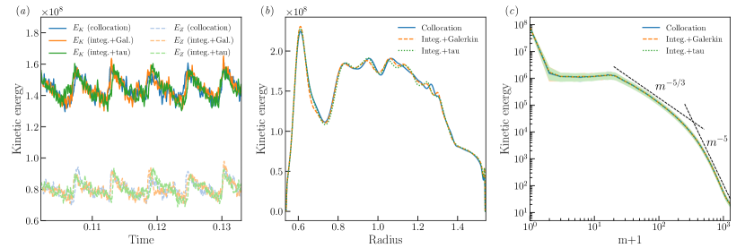
Figure 9: (a) Total $E_{K}$ and zonal $E_{Z}$ kinetic energy as a function of time for three numerical simulations with different radial discretisation schemes. (b) Time and azimuthally averaged kinetic energy as a function of radius. (c) Time-averaged kinetic energy spectra as a function of the wavenumber $m$. The shaded region correspond to one standard deviation of temporal fluctuations relative to the time averages. The simulations assume the following control parameters: $E=10^{-7}$, $Ra=2\times 10^{11}$ and $Pr=1$. The sparse cases have been computed with $\epsilon=10^{-3}$.

Table 4: Time-averaged diagnostics of three numerical simulations with $E=10^{-7}$, $Ra=2\times 10^{11}$ and $Pr=1$. The simulations have been computed with the BPR353 time scheme. The fourth column corresponds to the average time step size. The fifth and sixth column contain the time-average and the standard deviation of the total and the zonal kinetic energy, respectively. The last column corresponds to the total number of core hours spent to compute the time interval displayed in Fig. 9.

$r$ scheme	$(N_{r},N_{c},N_{m})$	$\epsilon$	$\overline{\delta t}$	$\overline{E_{K}}\pm\sigma(E_{K})$	$\overline{E_{Z}}\pm\sigma(E_{Z})$	Core hours
Collocation	$(641,641,1280)$	-	$2.623\times 10^{-8}$	$1.448\times 10^{8}\pm 6.281\times 10^{6}$	$8.075\times 10^{7}\pm 4.855\times 10^{6}$	$1.8\times 10^{4}$
Integ.+Galerkin	$(1025,682,1280)$	$10^{-3}$	$2.052\times 10^{-8}$	$1.448\times 10^{8}\pm 6.381\times 10^{6}$	$8.038\times 10^{7}\pm 4.884\times 10^{6}$	$3.7\times 10^{3}$
Integ.+tau	$(1025,682,1280)$	$10^{-3}$	$2.095\times 10^{-8}$	$1.443\times 10^{8}\pm 6.439\times 10^{6}$	$8.026\times 10^{7}\pm 4.661\times 10^{6}$,	$3.6\times 10^{3}$
Integ.+Galerkin	$(1025,682,1280)$	$10^{-4}$	$2.100\times 10^{-8}$	$1.452\times 10^{8}\pm 5.754\times 10^{6}$	$8.012\times 10^{7}\pm 4.211\times 10^{6}$	$3.8\times 10^{3}$
Integ.+tau	$(1025,682,1280)$	$10^{-4}$	$2.144\times 10^{-8}$	$1.450\times 10^{8}\pm 6.663\times 10^{6}$	$8.070\times 10^{7}\pm 5.231\times 10^{6}$	$3.6\times 10^{3}$

To pursue the code validation procedure, we now examine another physical setup which is not in the weakly nonlinear regime anymore with $E=10^{-7}$, $Pr=1$ and $Ra=2\times 10^{11}$, roughly 60 times the critical Rayleigh number. This corresponds to the setup that has been previously used to determine the Courant number of the different time schemes in § 4. To compare the different radial discretisation schemes, we first compute a simulation until a statistically steady-state has been reached. We then use this physical solution as a starting condition of several numerical simulations that use different radial discretisation schemes and two values of $\epsilon$ with the BPR353 time scheme. Since this is now a turbulent convection model, the time step size will change over time to satisfy the Courant condition (Eq. 40). To avoid the costly reconstruction of the matrices at each iteration, we adopt a time step size that is three quarter of the maximum eligible time step. The simulations are then computed over a timespan of roughly $0.03$ viscous time, which corresponds to more than $150$ turnover times.

Figure 9a shows the time evolution of the total and the zonal kinetic energy defined by

$$E_{K}=\dfrac{1}{2}\left\langle u_{s}^{2}+u_{\phi}^{2}\right\rangle=E_{Z}+2\pi\sum_{m=1}^{N_{m}}\int_{s_{i}}^{s_{o}}\left(|u_{s}^{m}|^{2}+|u_{\phi}^{m}|^{2}\right)s\,\mathrm{d}s\,,$$

where the zonal contribution is expressed by

$$E_{Z}=\dfrac{1}{2}\left\langle\overline{u_{\phi}}^{2}\right\rangle=\pi\int_{s_{i}}^{s_{0}}\overline{u_{\phi}}^{2}s\,\mathrm{d}s\,.$$

The three numerical simulations feature a very similar time evolution with roughly 50% of the energy content in the axisymmetric azimuthal motions. They show a quasi-periodic behaviour with quick energy increases followed by slower relaxations. This can be attributed to the time evolution of the zonal jets that slowly drift towards the inner boundary where they become unstable (Rotvig, 2007). Panels b and c of Fig. 9 show the time-average radial profiles and $m$ spectra of the kinetic energy, respectively. A good agreement is found between the three radial discretisation schemes. Typical of 2-D QG turbulence, an inverse energy cascade with a $m^{-5/3}$ slope takes place up to a typical lengthscale where the convective features are sheared apart by the zonal jets (here $m\simeq 20$, see Rhines, 1975). At smaller lengthscales the spectra transition to a $m^{-5}$ slope frequently observed in Rossby waves turbulence (e.g. Rhines, 1975; Schaeffer & Cardin, 2005b).

For a better quantification of the difference between the three radial schemes, Tab. 4 contains the time-average and the standard deviation of $E_{K}$ and $E_{Z}$ over the entire run time. Since dealiasing is also required in the radial direction when using a sparse Chebyshev formulation, the two cases that have been computed with the Chebyshev integration method have a larger number of radial grid points to ensure a number of Chebyshev modes comparable to the one used with the collocation method. Because of the change of the grid spacing (Eq. 40), this implies a decrease in the average time-step size. The time averages and standard deviation obtained for the three schemes and the two values of $\epsilon$ are found to agree within less than 1%. Given the unsteady nature of the solution, the differences in time step size and the limited time span considered for time averaging, it is not clear whether this difference can solely be attributed to the parametrisation of the Ekman pumping contribution. Notwithstanding this possible source of error, this comparison demonstrates that turbulent convection can be accurately modelled by an efficient sparse Chebyshev formulation with an acceptable error introduced by the Ekman pumping term approximation.

6.3 Turbulent QG convection

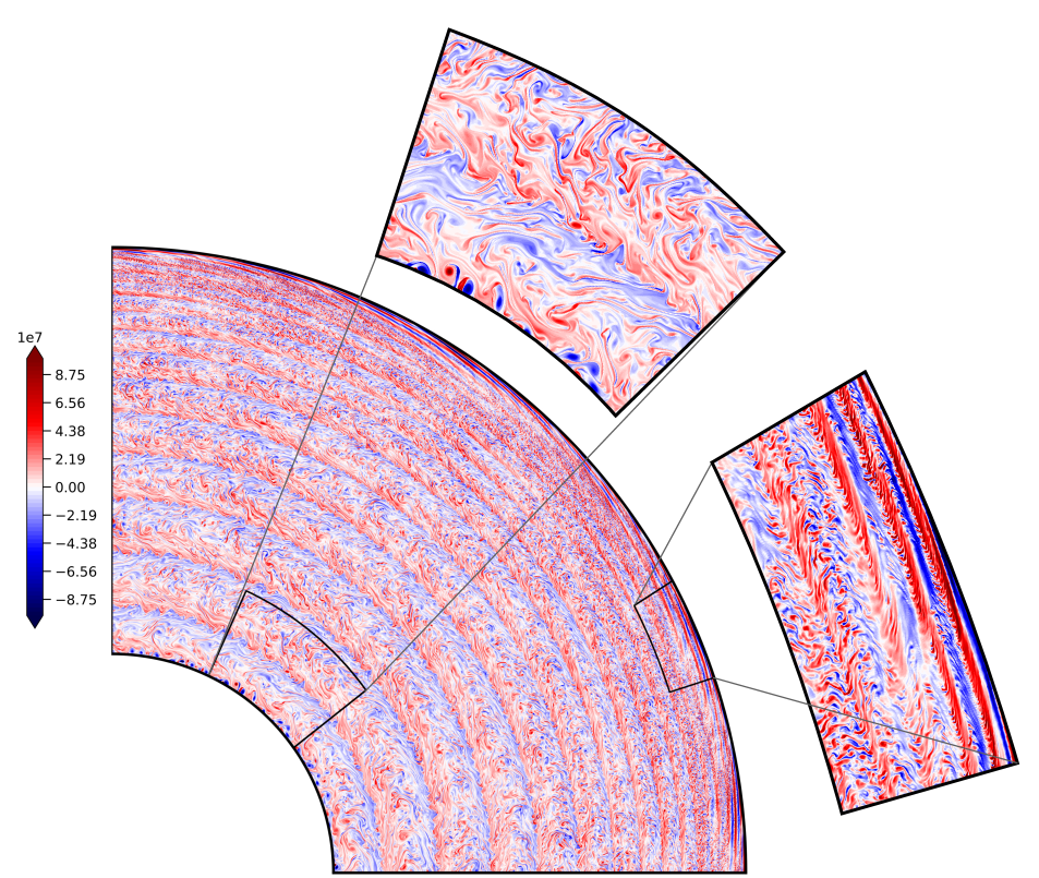
Figure 10: Snapshot of the axial vorticity for a numerical simulation with $E=10^{-9}$, $Ra=1.5\times 10^{14}$ and $Pr=1$. The Chebyshev integration formulation with a Galerkin approach to enforce the boundary condition has been employed to compute this numerical model. We use a spatial resolution $(N_{r},N_{m})=(6145,6144)$ and $\epsilon=10^{-4}$ for the approximated Ekman pumping term. For a better visualisation, only one quarter of the solution is displayed.

To check the ability of the spectral radial discretisation schemes to model turbulent QG convection, we consider a third numerical configuration with $E=10^{-9}$, $Ra=1.5\times 10^{14}$ and $Pr=1$. This corresponds to strongly supercritical convection ($Ra>100\,Ra_{c}$) at a very low Ekman number, a prerequisite to ensure that both large Reynolds and small Rossby numbers are reached at the same time. With the dimensionless units adopted in this study,

$$Re=\left[\dfrac{2E_{K}}{\pi(s_{o}^{2}-s_{i}^{2})}\right]^{1/2},\ Ro=Re\,E\,.$$

For these control parameters, convection develops in the so-called turbulent QG regime (e.g. Julien et al., 2012) with $Re\simeq 10^{5}$ and $Ro\simeq 10^{-4}$. Numerical models that operate at these extreme parameters demand a large number of grid points –here $(N_{r},N_{m})=(6145,6144)$– which becomes intractable for the Chebyshev collocation method. We hence only compute this model using the Chebyshev integration method combined with a Galerkin approach to enforce the boundary conditions. For this physical configuration, a time integration of roughly ten convective overturns requires about $10^{5}$ core hours.

Figure 10 shows a snapshot of the vorticity with two zoomed-in insets that emphasise the regions close the boundaries. The mixing of the potential vorticity $(\omega+2/E)/h$ by turbulent convective motions generates multiple zonal jets with alternated directions (e.g. Dritschel & McIntyre, 2008). This gives rise to a spatial separation of the vortical structures with alternated concentric rings of cyclonic ($\omega>0$) and anticyclonic ($\omega<0$) vorticity. The typical size of these zonal jets is usually well-predicted by the Rhines scale defined by $(Ro/|\beta|)^{1/2}$ (e.g. Rhines, 1975; Gastine et al., 2014; Verhoeven & Stellmach, 2014; Heimpel et al., 2016; Guervilly & Cardin, 2017). This lengthscale marks the separation between Rossby waves at larger scales and turbulent motions at smaller scales. Because of the increase of $|\beta|$ with the cylindrical radius $s$ in spherical geometry, the zonal jets are getting thinner outward. Close to the outer boundary, the dynamics becomes dominated by tilted vortices elongated in the azimuthal direction, a typical pattern of the propagation of thermal Rossby waves. Because of the steepening of $\beta$ at large radii, the vortex stretching term becomes the dominant source of vorticity there, such that the propagation of thermal Rossby waves takes over the nonlinear advective processes. This outer region is hence expected to shrink with an increase of the convective forcing (e.g. Guervilly & Cardin, 2017). At the interface between jets, the vortical structures are sheared apart into elongated filaments, indicating a direct cascade of enstrophy towards smaller scales.

7 Conclusion

In this study, we have presented a new open-source code, nicknamed pizza, dedicated to the study of rapidly-rotating convection under the 2-D spherical quasi-geostrophic approximation (e.g. Busse & Or, 1986; Aubert et al., 2003; Gillet & Jones, 2006). The code is available at https://github.com/magic-sph/pizza as a free software that can be used, modified, and redistributed under the terms of the GNU GPL v3 license. The radial discretisation relies on a decomposition in Fourier series in the azimuthal direction and in Chebyshev polynomials in the radial direction. For the latter, both a classical Chebyshev collocation method (e.g. Glatzmaier, 1984; Boyd, 2001) and a sparse integration method (e.g. Stellmach & Hansen, 2008; Muite, 2010; Marti et al., 2016) are supported. We adopt a pseudo-spectral approach where the nonlinear advective terms are treated in the physical space and transformed to the spectral space using fast discrete Fourier and Chebyshev transforms. pizza supports several implicit-explicit time schemes encompassing multi-step schemes as well as diagonally-implicit Runge-Kutta schemes (e.g. Ascher et al., 1997) that have been validated by convergence tests. The parallelisation strategy relies on a message-passing communication framework based on the MPI standard. The code has been tested and validated against onset of quasi-geostrophic convection.

The comparison of the two radial discretisation schemes has revealed the superiority of the Chebyshev integration method. In contrast to the collocation technique that requires the storage and the inversion of dense matrices, the integration method indeed only involves sparse operators. As a consequence, the memory requirements only grows with $\mathcal{O}(N_{r})$ and the operation count with $\mathcal{O}(N_{r}\ln N_{r})$ as compared to $\mathcal{O}(N_{r}^{2})$ when using a collocation approach. Multi-step and diagonally-implicit Runge-Kutta schemes have shown comparable efficiency, defined in this study by the ratio of the maximum CFL number over the numerical cost of one iteration. Additional parameter studies with various Reynolds and Rossby numbers are however required to assess the differences between both families of time integrators. We have found a good parallel scaling up to roughly four radial grid points per MPI task. This implies that large spatial resolution up to $\mathcal{O}(10^{4}\times 10^{4})$ grid points can be reached with a reasonable wall time if one uses several thousands of MPI tasks. Such large grid resolutions allows the study of turbulent quasi-geostrophic convection at low Ekman numbers. Preliminary results for a numerical model with $E=10^{-9}$, $Ra=1.5\times 10^{14}$ and $Pr=1$ shows the formation of multiple zonal jets, when both the Reynolds number is large $\mathcal{O}(10^{5})$ and the Rossby number is small $\mathcal{O}(10^{-4})$. This specific combination of $Re\gg 1$ and $Ro\ll 1$ is a prerequisite to study the turbulent quasi-geostrophic convection regime (Julien et al., 2012), an important milestone to better understand the internal dynamics of planetary interiors.

Future developments of the code include the implementation of the time-evolution of chemical composition to study double-diffusive convection under the spherical QG framework. On the longer term, the QG flow and temperature computed in the equatorial plane of the spherical shell will be coupled to an induction equation computed in the entire shell using classical 3-D pseudo-spectral discretisation (e.g. Schaeffer & Cardin, 2006).

Appendix A Direct solve of a bordered matrix

Suppose one wants to solve the following linear problem which involves a so-called bordered matrix $\mathcal{A}$

$$\mathcal{A}\psi=f,$$

where $\mathcal{A}$ comprises $p$ full top rows and a banded structure underneath. The matrix problem is sub-divided as follows

$$\left(\begin{array}[]{cc}A&B\\ C&D\end{array}\right)\left(\begin{array}[]{c}\psi_{1}\\ \psi_{2}\end{array}\right)=\left(\begin{array}[]{c}g\\ h\end{array}\right),$$

where $A$ is a full square matrix of size $(p\times p)$, $B$ is a full matrix of size $(p\times n-p)$, $C$ is a sparse matrix of size $(n-p\times p)$ and $D$ is a band matrix of size $(n-p)$ with a bandwidth $q$, $q$ being the total number of bands. One first solves the two following banded linear problems

$$Dx=h\,,\quad Dy=C\,.$$

The LU factorisation of the band matrix $D$ requires $\mathcal{O}(q^{2}\,n)$ operations, while the solve requires $\mathcal{O}(q\,n)$ operations (e.g. Boyd, 2001, Appendix B2). We then assemble the Schur complement of the banded block $D$

$$M=A-BD^{-1}C=A-By\,,$$

before solving the small dense problem of size $(p,p)$

$$M\psi_{1}=g-Bx\,.$$

This requires $\mathcal{O}(p^{3})$ operations for the LU factorisation and $\mathcal{O}(p^{2})$ for the solve. This cost remains negligible as long as $p\ll n$, which is the case for the linear problems considered in the Chebyshev integration method. We finally evaluate

$$\psi_{2}=x-y\,\psi_{1}\,,$$

to assemble the final solution given by $\psi=(\psi_{1},\psi_{2})^{T}$.

Appendix B Galerkin basis for streamfunction boundary conditions

In this section, we derive a Galerkin basis function for the following combination of boundary conditions that is used in the Chebyshev integration method for the streamfunction equation

$$\varPsi=\dfrac{\partial\varPsi}{\partial s}=0,\quad\text{for}\quad s=s_{i}\,,$$

and

$$\varPsi=\dfrac{\partial^{3}\varPsi}{\partial s^{3}}=0,\quad\text{for}\quad s=s_{o}\,.$$

We start by defining the following ansatz for the Galerkin set

$$\phi_{n}(x)=\sum_{i=0}^{4}\gamma_{i}^{n}\,T_{n+i}(x)\,.$$

Following McFadden et al. (1990) and Julien & Watson (2009) we then make use of the tau boundary conditions (Eqs. 19,20 and 31) to form the following system of equations

$$\phi_{n}(1) =\sum_{i=0}^{4}\gamma_{i}^{n} =0,$$

$$\phi_{n}(-1) =\sum_{i=0}^{4}(-1)^{i}\gamma_{i}^{n} =0,$$

$$\dfrac{\partial^{3}\phi_{n}}{\partial x^{3}}(1) =\sum_{i=0}^{4}(n+i)^{2}[(n+i)^{2}-1][(n+i)^{2}-4]\gamma_{i}^{n} =0,$$

$$\dfrac{\partial\phi_{n}}{\partial x}(-1) =\sum_{i=0}^{4}(-1)^{i+1}(n+i)^{2}\gamma_{i}^{n} =0,$$

Since there are only four equations for five unknowns, there is a degree of freedom in the determination of the coefficients. We thus choose in following

$$\gamma_{0}^{n}=1,$$

which yields the following identities for the other coefficients:

$$\gamma_{1}^{n} =\frac{8\left(n+1\right)\left(n^{2}+4n+5\right)}{2n^{4}+20n^{3}+78n^{2}+140n+95},$$

$$\gamma_{2}^{n} =-\frac{2\left(n+2\right)\left(2n^{4}+16n^{3}+58n^{2}+104n+75\right)}{\left(n+3\right)\left(2n^{4}+20n^{3}+78n^{2}+140n+95\right)},$$

$$\gamma_{3}^{n} =-\frac{8\left(n+1\right)\left(n^{2}+4n+5\right)}{2n^{4}+20n^{3}+78n^{2}+140n+95},$$

and

$$\gamma_{4}^{n}=\frac{\left(n+1\right)\left(2n^{4}+12n^{3}+30n^{2}+36n+15\right)}{\left(n+3\right)\left(2n^{4}+20n^{3}+78n^{2}+140n+95\right)}\,.$$