Directional Regularized Tensor Modeling for Video Rain Streaks Removal

Abstract

Outdoor videos sometimes contain unexpected rain streaks due to the rainy weather, which bring negative effects on subsequent computer vision applications, e.g., video surveillance, object recognition and tracking, etc. In this paper, we propose a directional regularized tensor-based video deraining model by taking into consideration the arbitrary direction of rain streaks. In particular, the sparsity of rain streaks in spatial and derivative domains, the spatiotemporal sparsity and low-rank property of video background are incorporated into the proposed method. Different from many previous methods under the assumption of vertically falling rain streaks, we consider a more realistic assumption that all the rain streaks in a video fall in an approximately similar arbitrary direction. The resulting complicated optimization problem will be effectively solved through an alternating direction method. Comprehensive experiments on both synthetic and realistic datasets have demonstrated the superiority of the proposed deraining method.

Index Terms—  Video restoration, rain removal, tensor modeling, directional total variation, ADMM

1 Introduction

The existence of undesirable rain streaks in images or videos has a significant negative impact on outdoor visual system, such as object detection [1, 2], event detection [3], object recognition [4] and tracking [5]. Rain streaks removal from videos or images is thus an important issue and has been investigated extensively in computer vision research.

Inspired by the pioneering deraining research [6], a large amount of rain streaks removal methods have been proposed to enhance imaging performance. The current methods can be divided into two categories: single-image-based methods and video-based methods. For single-image rain removal, Kang et al. [7] decomposed an input hazy image into low- and high-frequency components, and proposed to separate the rain streaks from the high-frequency component using sparse coding. Luo et al. [8] removed rain streaks from a single image via highly discriminative sparse coding. Li et al. [9] utilized patch-based Gaussian mixture model (GMM) prior to restore a rain-free image from its rainy version. The restored images, however, often suffer from loss of fine details. For video rain streaks removal, Garg et al. [6] developed a comprehensive rain detection method based on photometric and dynamic models related to rain streaks. Kim et al. [10] first estimated an initial rain map using temporal correlation, and then restored the rain-free video by low-rank matrix completion. Jiang et al. [11] presented a tensor-based video rain streaks removal model by considering the discriminatively intrinsic characteristics of video background and rain streaks. Wei et al. [12] proposed to improve deraining results by integrating with the spatiotemporal smoothness of moving objects and low-rank structure of video background. Please refer to Ref. [13] for a survey work on rain streaks removal.

More recently, effective deep learning architectures [14, 15, 16, 17, 18] have achieved impressive results for both single-image and video deraining. It should be pointed out that the deraining results are strongly depended on the volume and diversity of training datasets. To make deraining more flexible, mainly inspired by the work of [11], we will propose a directional regularized tensor-based video rain streaks removal model based on the assumption of arbitrary direction of rain streaks. Its satisfactory deraining performance benefits from the directional regularizer and tensor modeling.

2 Problem Formulation

The rainy video $\mathcal{O}\in\mathbb{R}^{m\times n\times t}$ can be modeled as a linear superimposition of the desired unknown video background $\mathcal{B}\in\mathbb{R}^{m\times n\times t}$ and the rain streaks $\mathcal{R}\in\mathbb{R}^{m\times n\times t}$, i.e.,

$$\mathcal{O}=\mathcal{B}+\mathcal{R}.$$ (1)

The goal of deraining is to decompose the desired video background $\mathcal{B}$ and rain streaks $\mathcal{R}$ from the input rainy video $\mathcal{O}$. This decomposition process is an ill-posed inverse problem. The (statistical) priors on both $\mathcal{B}$ and $\mathcal{R}$ should be considered to regularize the decomposition process. By introducing priors on both $\mathcal{B}$ and $\mathcal{R}$, Ref. [11] proposed a tensor-based variational model for video rain streaks removal, i.e.,

$$\min_{\mathcal{B},\mathcal{R}}~{}\alpha_{1}\|\nabla_{y}\mathcal{R}\|_{1}+\alpha_{2}\|\mathcal{R}\|_{1}+\alpha_{3}\|\nabla_{x}\mathcal{B}\|_{1}+\alpha_{4}\|\nabla_{t}\mathcal{B}\|_{1}+\mathrm{rank}(\mathcal{B})$$

$$~{}~{}\mathrm{s.t.}~{}~{}~{}\mathcal{O}=\mathcal{B}+\mathcal{R},~{}\mathcal{B},\mathcal{R}\geq 0,$$ (2)

where $\nabla_{x},\nabla_{y},\nabla_{t}$ denote three unidirectional TV operators with respects of vertical, horizontal and temporal directions.

The tensor-based variational model (2) is based on the assumption of vertical direction of falling raindrops. It is infrequent in realistic scenarios due to the influence of wind and other factors. Meanwhile, this variational model (2) only considers the sparsity of vertical derivatives of rain streaks and uses the traditional TV regularizer $\|\nabla_{y}\mathcal{R}\|_{1}$. The L1-norm regularizer $\|\mathcal{R}\|_{1}$ is related to the assumption that the magnitudes of rain streaks are commonly sparse. Since the horizontal and temporal derivatives of video background are assumed to be sparse, TV regularizers $\|\nabla_{x}\mathcal{B}\|_{1}$ and $\|\nabla_{t}\mathcal{B}\|_{1}$ are used to regularize the deraining process. By using the spatio-temporal coherences of video data, tensor modeling $\mathrm{rank}(\mathcal{B})$ is introduced to further enhance imaging performance.

3 Directional Regularized Tensor Modeling

3.1 DTV Regularized Tensor Decomposition Model

The falling directions of raindrops are essentially spatially variant in realistic videos. For the sake of simplicity, we assume that all rain streaks fall in an approximately identical direction. We propose to develop a directional regularized tensor modeling for removing video rain streaks as follows

$$\min_{\mathcal{B},\mathcal{R}}~{}\alpha_{1}\|\nabla_{d}\mathcal{R}\|_{1}+\alpha_{2}\|\mathcal{R}\|_{1}+\alpha_{3}\|\nabla_{x}\mathcal{B}\|_{1}$$

$$~{}~{}~{}~{}~{}~{}~{}~{}~{}~{}~{}~{}~{}~{}~{}~{}~{}~{}~{}~{}~{}~{}~{}~{}~{}~{}~{}~{}+\alpha_{4}\|\nabla_{y}\mathcal{B}\|_{1}+\alpha_{5}\|\nabla_{t}\mathcal{B}\|_{1}+\mathrm{rank}(\mathcal{B})$$

$$~{}~{}\mathrm{s.t.}~{}~{}~{}\mathcal{O}=\mathcal{B}+\mathcal{R},~{}\mathcal{B},\mathcal{R}\geq 0,$$ (3)

where $d$ denotes the falling direction of rain streaks, $\nabla_{d}$ is the directional total variation (DTV) operator. We will detailedly discuss the potential reasons why introducing different regularization terms in Eq. (3.1).

Sparsity of Rain Streaks in Spatial and Derivative Domains In the case of light rain, rain streaks can be sparsely represented in both spatial and derivative domains. As the rainfall intensity becomes higher, it is better to consider the sparsity of rain streaks in derivative domain. The image derivatives are calculated along the falling (not vertical) direction of rain streaks. In contrast, Jiang et al. [11] only considers the vertical direction which is an invalid assumption in practice. The L1-norm regularizer $\|\mathcal{R}\|_{1}$ and DTV regularizer $\|\nabla_{d}\mathcal{R}\|_{1}$ are adopted to model the sparsity of rain streaks in spatial and derivative domains, respectively.

Sparsity of Video Intensities in Spatial and Temporal Domains Both vertical and horizontal derivatives in outdoor images can be well distributed as the Laplacian distribution. TV regularizer is essentially related to the assumption of Laplacian prior [19]. There commonly exists high similarity between consecutive frames within one video. The distribution of differences between any two consecutive frames (i.e., along temporal direction) can also be modeled by a Laplacian prior. Therefore, TV regularizers $\|\nabla_{x}\mathcal{B}\|_{1}$, $\|\nabla_{y}\mathcal{B}\|_{1}$ and $\|\nabla_{t}\mathcal{B}\|_{1}$ are used to model the sparsity of video intensities in vertical, horizontal and temporal directions, respectively.

Tensor Structures in Video Intensities Spatial self-similarities within each frame and temporal similarities between any two consecutive frames can be visually observed, especially for video generated by static camera or with static background. Recently, low-rank [10, 20, 21] and tensor [11] modeling have significantly improved the deraining performance. By exploiting the tensor structures in video intensities [11], our model (3.1) also minimizes the rank of $\mathcal{B}$ to promote the decomposition of video background and rain streaks.

3.2 Numerical Optimization

The alternating direction method of multipliers (ADMM) framework [22] will be used to effectively solve the complicated unconstrained optimization problem (3.1). By introducing several intermediate variables, we can reformulate (3.1) as the following equivalent constrained version

$$\min_{\mathcal{R},\mathcal{D},\mathcal{S},\mathcal{X},\mathcal{Y},\mathcal{T},\mathcal{L}}~{}\alpha_{1}\|\nabla_{d}\mathcal{D}\|_{1}+\alpha_{2}\|\mathcal{S}\|_{1}+\alpha_{3}\|\mathcal{X}\|_{1}$$

$$~{}~{}~{}~{}~{}~{}~{}~{}~{}~{}~{}~{}~{}~{}~{}~{}~{}~{}~{}~{}~{}~{}~{}~{}~{}~{}~{}~{}~{}~{}~{}~{}~{}~{}~{}~{}~{}~{}~{}~{}+\alpha_{4}\|\mathcal{Y}\|_{1}+\alpha_{5}\|\mathcal{T}\|_{1}+\|\mathcal{L}\|_{*}$$

$$~{}~{}~{}~{}~{}~{}~{}~{}~{}~{}\mathrm{s.t.}~{}~{}~{}\mathcal{D}=\mathcal{R},~{}\mathcal{S}=\mathcal{R},~{}\mathcal{X}=\nabla_{x}(\mathcal{O}-\mathcal{R}),$$

$$~{}~{}~{}~{}~{}~{}~{}~{}~{}~{}~{}~{}~{}~{}~{}~{}~{}~{}~{}\mathcal{Y}=\nabla_{y}(\mathcal{O}-\mathcal{R}),~{}\mathcal{T}=\nabla_{t}(\mathcal{O}-\mathcal{R}),$$

$$~{}~{}~{}~{}~{}~{}~{}~{}~{}~{}~{}~{}~{}~{}~{}~{}~{}~{}~{}\mathcal{L}=\mathcal{O}-\mathcal{R},~{}\mathcal{O}\geq\mathcal{R}\geq 0$$ (4)

whose augmented Lagrangian function $\mathcal{L}_{\mathcal{A}}$ is given by

$$\mathcal{L}_{\mathcal{A}}=\alpha_{1}\|\nabla_{d}\mathcal{D}\|_{1}+\alpha_{2}\|\mathcal{S}\|_{1}+\alpha_{3}\|\mathcal{X}\|_{1}+\alpha_{4}\|\mathcal{Y}\|_{1}+\alpha_{5}\|\mathcal{T}\|_{1}$$

$$+\|\mathcal{L}\|_{*}+\frac{\beta_{1}}{2}\Big{\|}\mathcal{D}-\mathcal{R}-\frac{\Lambda_{1}}{\beta_{1}}\Big{\|}_{F}^{2}+\frac{\beta_{2}}{2}\Big{\|}\mathcal{S}-\mathcal{R}-\frac{\Lambda_{2}}{\beta_{2}}\Big{\|}_{F}^{2}$$

$$+\frac{\beta_{3}}{2}\Big{\|}\mathcal{X}-\nabla_{x}(\mathcal{O}-\mathcal{R})-\frac{\Lambda_{3}}{\beta_{3}}\Big{\|}_{F}^{2}+\frac{\beta_{4}}{2}\Big{\|}\mathcal{Y}-\nabla_{y}(\mathcal{O}-\mathcal{R})-\frac{\Lambda_{4}}{\beta_{4}}\Big{\|}_{F}^{2}$$

$$+\frac{\beta_{5}}{2}\Big{\|}\mathcal{T}-\nabla_{t}(\mathcal{O}-\mathcal{R})-\frac{\Lambda_{5}}{\beta_{5}}\Big{\|}_{F}^{2}+\frac{\beta_{6}}{2}\Big{\|}\mathcal{L}-(\mathcal{O}-\mathcal{R})-\frac{\Lambda_{6}}{\beta_{6}}\Big{\|}_{F}^{2}$$

where $\Lambda=[\Lambda_{1},\Lambda_{2},\cdots,\Lambda_{6}]$ are Lagrangian multipliers and $\beta=[\beta_{1},\beta_{2},\cdots,\beta_{6}]$ are positive parameters. Within our optimization framework, ADMM minimizes $\mathcal{L}_{\mathcal{A}}$ over $\mathcal{R}$, $\mathcal{D}$, $\mathcal{S}$, $\mathcal{X}$, $\mathcal{Y}$, $\mathcal{T}$ and $\mathcal{L}$ leading to subproblems whose solutions could be efficiently obtained using simple numerical methods.

$\mathcal{D}$-subproblem: Within the ADMM framework, the $\mathcal{D}$-subproblem can be formulated as follows

$$\min_{D}\alpha_{1}\|\nabla_{d}\mathcal{D}\|_{1}+\frac{\beta_{1}}{2}\|\mathcal{R}-\mathcal{D}+\frac{\Lambda_{1}}{\beta_{1}}\|_{F}^{2}.$$ (5)

The falling direction $d$ of rain streaks is pre-estimated directly using the Fourier transform method [23]. The generalized proximal operator introduced in [24] is adopted to effectively handle the nonsmooth optimization problem (5).

$\left(\mathcal{S},\mathcal{X},\mathcal{Y},\mathcal{T}\right)$-subproblems: For $\mathcal{S}$-subproblem, the minimization problem can be formulated as follows

$$\min_{S}\alpha_{2}\|\mathcal{S}\|_{1}+\frac{\beta_{2}}{2}\|\mathcal{R}-\mathcal{S}+\frac{\Lambda_{2}}{\beta_{2}}\|_{F}^{2},$$ (6)

which has a closed-form solution through the following soft-thresholding operator

$$\mathcal{S}^{(t+1)}=\mathrm{Soft}_{{\alpha_{2}}/{\beta_{2}}}\left(\mathcal{R}^{(t)}+{\Lambda_{2}^{(t)}}/{\beta_{2}}\right),$$ (7)

with $\mathrm{Soft}_{{\alpha}/{\beta}}(\cdot)$ being defined as $\mathrm{Soft}_{{\alpha}/{\beta}}\left(x\right)=\mathrm{sign}(x)\circ\max(\left|x\right|-{\alpha}/{\beta},0)$. Analogous to the $\mathcal{S}$-subproblem (6), the solutions $\mathcal{X},\mathcal{Y},\mathcal{T}$ can be updated as follows

$$\mathcal{X}^{(t+1)} =\mathrm{Soft}_{{\alpha_{3}}/{\beta_{3}}}\left(\nabla_{x}(\mathcal{O}-\mathcal{R}^{(t)})+{\Lambda_{3}^{(t)}}/{\beta_{3}}\right),$$ (8)

$$\mathcal{Y}^{(t+1)} =\mathrm{Soft}_{{\alpha_{4}}/{\beta_{4}}}\left(\nabla_{y}(\mathcal{O}-\mathcal{R}^{(t)})+{\Lambda_{4}^{(t)}}/{\beta_{4}}\right),$$ (9)

$$\mathcal{T}^{(t+1)} =\mathrm{Soft}_{{\alpha_{5}}/{\beta_{5}}}\left(\nabla_{t}(\mathcal{O}-\mathcal{R}^{(t)})+{\Lambda_{5}^{(t)}}/{\beta_{5}}\right).$$ (10)

$\mathcal{L}$-subproblem: The $\mathcal{L}$-subproblem is given by

$$\min_{\mathcal{L}}\|\mathcal{L}\|_{*}+\frac{\beta_{6}}{2}\|\mathcal{O}-\mathcal{R}-\mathcal{L}+\frac{\Lambda_{6}}{\beta_{6}}\|_{F}^{2},$$ (11)

where the tensor nuclear norm is defined as $\left\|\mathcal{X}\right\|_{*}=\sum_{i=1}^{n}\left\|\mathbf{X}_{i}\right\|_{*}$ with $\mathbf{X}_{i}=\mathrm{unfold}_{i}(\mathcal{X})$. The solution $\mathcal{L}$ of (11) is given by

$$\mathcal{L}^{(t+1)}=\sum\nolimits_{i=1}^{3}\frac{1}{3}\mathrm{Fold}_{i}\big{(}\mathbf{L}_{(i)}^{(t+1)}\big{)},$$ (12)

where $\mathbf{L}_{(i)}^{(t+1)}=\mathcal{Q}_{\frac{1}{\beta_{6}}}\left(\mathbf{B}_{(i)}^{(t)}+{\Lambda_{(i)}^{(t)}}/{\beta_{6}}\right)$ and $\mathcal{Q}_{\frac{1}{\beta_{6}}}(\mathbf{X})$ denotes the soft-thresholding to the singular values of $\mathbf{X}$.

$\mathcal{R}$-subproblem: Finally, the $\mathcal{R}$-subproblem is given by

$$\min_{\mathcal{R}}~{}\frac{\beta_{1}}{2}\|\mathcal{R}-\mathcal{D}\|_{F}^{2}+\frac{\beta_{2}}{2}\|\mathcal{R}-\mathcal{S}\|_{F}^{2}$$ (13)

$$+\frac{\beta_{3}}{2}\Big{\|}\mathcal{X}-\nabla_{x}(\mathcal{O}-\mathcal{R})-\frac{\Lambda_{3}}{\beta_{3}}\Big{\|}_{F}^{2}+\frac{\beta_{4}}{2}\Big{\|}\mathcal{Y}-\nabla_{y}(\mathcal{O}-\mathcal{R})-\frac{\Lambda_{4}}{\beta_{4}}\Big{\|}_{F}^{2}$$

$$+\frac{\beta_{5}}{2}\Big{\|}\mathcal{T}-\nabla_{t}(\mathcal{O}-\mathcal{R})-\frac{\Lambda_{5}}{\beta_{5}}\Big{\|}_{F}^{2}+\frac{\beta_{6}}{2}\Big{\|}\mathcal{L}-(\mathcal{O}-\mathcal{R})-\frac{\Lambda_{6}}{\beta_{6}}\Big{\|}_{F}^{2},$$

which has the following closed-form solution

$$\mathcal{R}^{(t+1)}=\mathcal{F}^{-1}\left({\mathcal{F}(\mathcal{K}_{1})}/{\mathcal{F}(\mathcal{K}_{2})}\right),$$ (14)

where $\mathcal{F}$ and $\mathcal{F}^{-1}$ denote the fast Fourier transform (FFT) and its inverse, $\mathcal{K}_{1}=\beta_{1}\mathcal{D}^{(t+1)}-\Lambda_{1}^{t}+\beta_{2}\mathcal{S}^{(t+1)}-\Lambda_{2}^{(t)}+\nabla_{x}^{T}(\beta_{3}\nabla_{x}\mathcal{O}-\beta_{3}\mathcal{X}^{(t+1)}+\Lambda_{3}^{(t)})+\nabla_{y}^{T}(\beta_{4}\nabla_{y}\mathcal{O}-\beta_{4}\mathcal{Y}^{(t+1)}+\Lambda_{4}^{(t)})+\nabla_{t}^{T}(\beta_{5}\nabla_{t}\mathcal{O}-\beta_{5}\mathcal{T}^{(t+1)}+\Lambda_{5}^{(t)})+\beta_{6}(\mathcal{O}-\mathcal{L}^{(t+1)})+\Lambda_{6}^{(t)}$ and $\mathcal{K}_{2}=(1+\beta_{1}+\beta_{2})\mathcal{I}+\beta_{3}\nabla_{x}^{T}\nabla_{x}+\beta_{4}\nabla_{y}^{T}\nabla_{y}+\beta_{5}\nabla_{t}^{T}\nabla_{t}$.

$\Lambda$ update: During each iteration, the Lagrangian multipliers $\Lambda$ are updated using $\Lambda_{1}^{(t+1)}=\Lambda_{1}^{(t)}+\beta_{1}(\mathcal{R}^{(t+1)}-\mathcal{D}^{(t+1)})$, $\Lambda_{2}^{(t+1)}=\Lambda_{2}^{(t)}+\beta_{2}(\mathcal{R}^{(t+1)}-\mathcal{S}^{(t+1)})$, $\Lambda_{3}^{(t+1)}=\Lambda_{3}^{(t)}+\beta_{3}(\nabla_{x}(\mathcal{O}-\mathcal{R}^{(t+1)})-\mathcal{X}^{(t+1)})$, $\Lambda_{4}^{(t+1)}=\Lambda_{4}^{(t)}+\beta_{4}(\nabla_{y}(\mathcal{O}-\mathcal{R}^{(t+1)})-\mathcal{Y}^{(t+1)})$, $\Lambda_{5}^{(t+1)}=\Lambda_{5}^{(t)}+\beta_{5}(\nabla_{t}(\mathcal{O}-\mathcal{R}^{(t+1)})-\mathcal{T}^{(t+1)})$ and $\Lambda_{6}^{(t+1)}=\Lambda_{6}^{(t)}+\beta_{6}(\mathcal{O}-\mathcal{R}^{(t+1)}-\mathcal{L}^{(t+1)})$.

Table 1: Quantitative comparisons of rain streaks removal on five different synthetic videos.

Rain Types		Heavy								Light
		45 Degrees				60 Degrees				45 Degrees				60 Degrees
		PSNR($\mathcal{B}$)	SSIM($\mathcal{B}$)	SSIM($\mathcal{R}$)	RES($\mathcal{B}$)	PSNR($\mathcal{B}$)	SSIM($\mathcal{B}$)	SSIM($\mathcal{R}$)	RES($\mathcal{B}$)	PSNR($\mathcal{B}$)	SSIM($\mathcal{B}$)	SSIM($\mathcal{R}$)	RES($\mathcal{B}$)	PSNR($\mathcal{B}$)	SSIM($\mathcal{B}$)	SSIM($\mathcal{R}$)	RES($\mathcal{B}$)
Foreman	Rainy	27.519	0.719	-	33.211	27.537	0.721	-	33.150	36.279	0.828	-	12.126	36.632	0.832	-	11.650
	Luo et al. [8]	29.693	0.721	0.685	25.858	30.006	0.728	0.631	24.959	35.115	0.822	0.251	13.868	34.996	0.827	0.273	14.058
	Li et al. [9]	31.773	0.771	0.382	20.361	31.827	0.771	0.377	20.237	34.914	0.838	0.230	14.187	34.911	0.836	0.238	14.190
	Jiang et al. [11]	30.008	0.788	0.316	24.996	30.57	0.813	0.383	23.408	38.009	0.876	0.438	10.355	38.970	0.903	0.533	9.460
	Ours	31.853	0.852	0.536	20.226	31.841	0.852	0.531	20.269	39.401	0.947	0.669	9.399	39.388	0.941	0.645	9.426
Girl	Rainy	28.596	0.732	-	48.881	28.588	0.731	-	48.920	37.348	0.867	-	17.859	38.141	0.867	-	19.965
	Luoet al. [8]	30.631	0.745	0.821	38.670	30.534	0.743	0.831	39.119	37.154	0.865	0.116	18.265	37.088	0.867	0.013	18.397
	Li et al. [9]	32.411	0.719	0.309	31.507	32.474	0.722	0.301	31.278	34.468	0.775	0.229	24.854	34.479	0.777	0.230	24.829
	Jiang et al. [11]	31.392	0.834	0.346	35.828	32.018	0.852	0.418	33.445	38.809	0.936	0.636	17.082	41.094	0.940	0.718	16.504
	Ours	33.083	0.882	0.559	29.936	32.906	0.881	0.560	30.522	38.601	0.976	0.823	18.137	38.016	0.975	0.817	19.140
Highway	Rainy	28.178	0.530	-	30.790	28.154	0.527	-	30.883	36.946	0.712	-	11.245	36.813	0.708	-	11.406
	Luo et al. [8]	30.564	0.549	0.735	23.404	31.06	0.559	0.638	22.109	37.589	0.712	0.246	10.435	37.541	0.714	0.106	10.482
	Li et al. [9]	30.755	0.543	0.390	22.883	30.741	0.543	0.390	22.926	32.926	0.674	0.108	17.815	32.998	0.677	0.107	17.670
	Jiang et al. [11]	30.839	0.647	0.325	22.711	31.362	0.673	0.390	21.394	40.154	0.797	0.540	8.096	41.292	0.828	0.632	7.204
	Ours	33.047	0.723	0.544	17.638	33.486	0.720	0.615	16.868	44.999	0.901	0.788	5.057	44.711	0.893	0.772	5.204
Truck	Rainy	27.329	0.686	-	56.552	27.345	0.687	-	56.452	36.303	0.824	-	20.151	36.204	0.821	-	20.361
	Luo et al. [8]	30.882	0.700	0.529	37.582	31.962	0.720	0.327	33.216	33.332	0.813	0.338	28.465	32.644	0.814	0.409	30.701
	Li et al. [9]	30.842	0.704	0.297	37.739	30.866	0.706	0.303	37.639	31.831	0.784	0.136	33.674	31.821	0.784	0.137	33.715
	Jiang et al. [11]	28.919	0.749	0.174	47.213	29.470	0.775	0.245	44.338	38.656	0.876	0.398	15.711	39.852	0.899	0.548	13.816
	Ours	30.138	0.840	0.620	41.164	30.514	0.852	0.628	39.438	45.141	0.968	0.832	8.194	44.141	0.959	0.807	9.003
Waterfall	Rainy	27.688	0.804	-	32.577	27.709	0.804	-	32.503	36.445	0.914	-	11.910	36.783	0.920	-	11.451
	Luo et al. [8]	30.649	0.796	0.349	23.172	30.848	0.798	0.283	22.653	30.454	0.893	0.527	21.986	31.114	0.900	0.524	21.986
	Li et al. [9]	31.149	0.689	0.188	21.862	31.134	0.691	0.194	21.898	31.085	0.737	0.127	22.030	30.991	0.736	0.124	22.264
	Jiang et al. [11]	29.346	0.858	0.181	26.959	29.848	0.877	0.241	25.448	38.332	0.938	0.347	9.783	39.458	0.952	0.459	8.689
	Ours	32.510	0.919	0.581	18.766	32.568	0.920	0.581	18.643	41.531	0.975	0.699	6.960	41.456	0.974	0.670	7.020

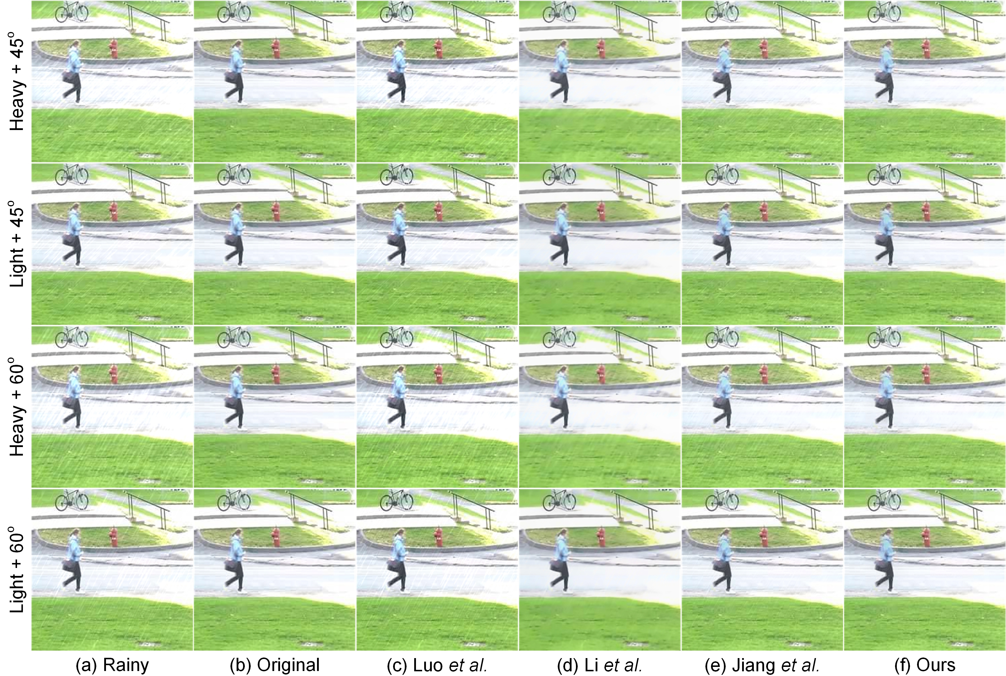
Fig. 1: Comparisons of deraining results on one frame extracted from the synthetic “Girl” video under different rainy conditions. From left to right: (a) rainy images, (b) original rain-free images, restored images generated by (c) Luo et al. [8], (d) Li et al. [9], (e) Jiang et al. [11] and (f) ours.

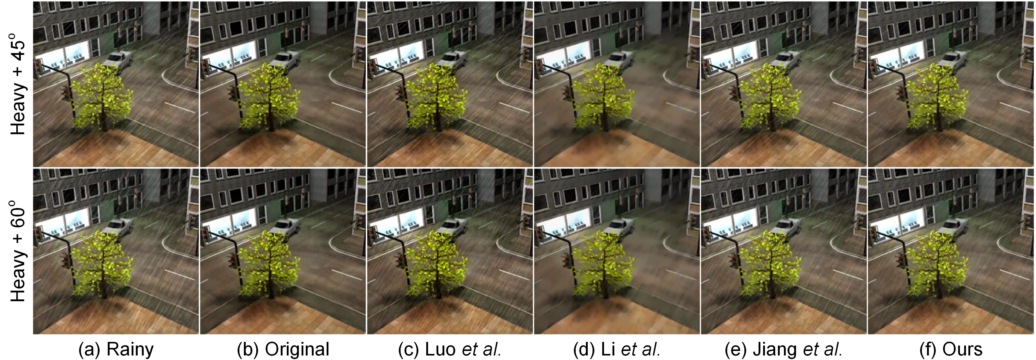
Fig. 2: Comparisons of deraining results on one frame extracted from the synthetic “Truck” video under different rainy conditions. From left to right: (a) rainy images, (b) original rain-free images, restored images generated by (c) Luo et al. [8], (d) Li et al. [9], (e) Jiang et al. [11] and (f) ours.

4 Experimental Results and Discussion

To verify the effectiveness of the proposed method, we compare our method with several advanced deraining methods, including sparse coding method Luo et al. [8], layer priors-based method Li et al. [9], and tensor-based method Jiang et al. [11]. For synthetic experiments, the falling directions of rain streaks were randomly selected between $[40~{}50]$ or $[55~{}65]$. In numerical experiments, the regularization parameters $\{\alpha_{1},\alpha_{2},\cdots,\alpha_{5}\}$ were manually selected from $\{10^{1},10^{2},10^{3}\}$ and $\{\beta_{1},\beta_{2},\cdots,\beta_{6}\}$ were set to be $50$. The effectiveness of these manually selected parameters has been illustrated through comprehensive deraining experiments. Our Matlab source code is available at https://github.com/Snowfallingplum/rain-streaks-removal.

4.1 Synthetic Experiments

The rain streaks with different types are manually generated and incorporated into the original video backgrounds. Objective image quality metrics, i.e., PSNR, SSIM and residual error (RES), are selected to quantitatively evaluate the deraining results. Table 1 detailedly depicts the quantitative results for five synthetic datasets. It is shown that our method generates the best evaluation results under consideration in most of the cases. Its superior performance is further confirmed in Figs. 1 and 2. The degrees $45^{\circ}$ and $60^{\circ}$ are the average falling directions of rain streaks. The restored images generated by Luo et al. [8] still suffer from rain streaks remaining leading to visual quality degradation. Li et al. [9] could effectively reduce rain effects but tend to oversmooth fine details. Compared with Jiang et al. [11], our method is able to effectively remove more rain streaks while preserving fine details.

4.2 Realistic Experiments

In the realistic experiments, it is impossible to accurately obtain the video backgrounds for quantitative evaluation. In theory, deraining methods should preserve fine details while sufficiently removing rain streaks. Fig. 3 illustrates the deraining results on three different frames extracted from the realistic “The Grandmaster” video. Due to the nonvertical direction of falling raindrops, other three competing methods fail to effectively remove the undesirable rain streaks. In contrast, the proposed method fits this realistic scene well and removes almost all rain streaks. Its superior performance benefits from the DTV regularizer and tensor modeling.

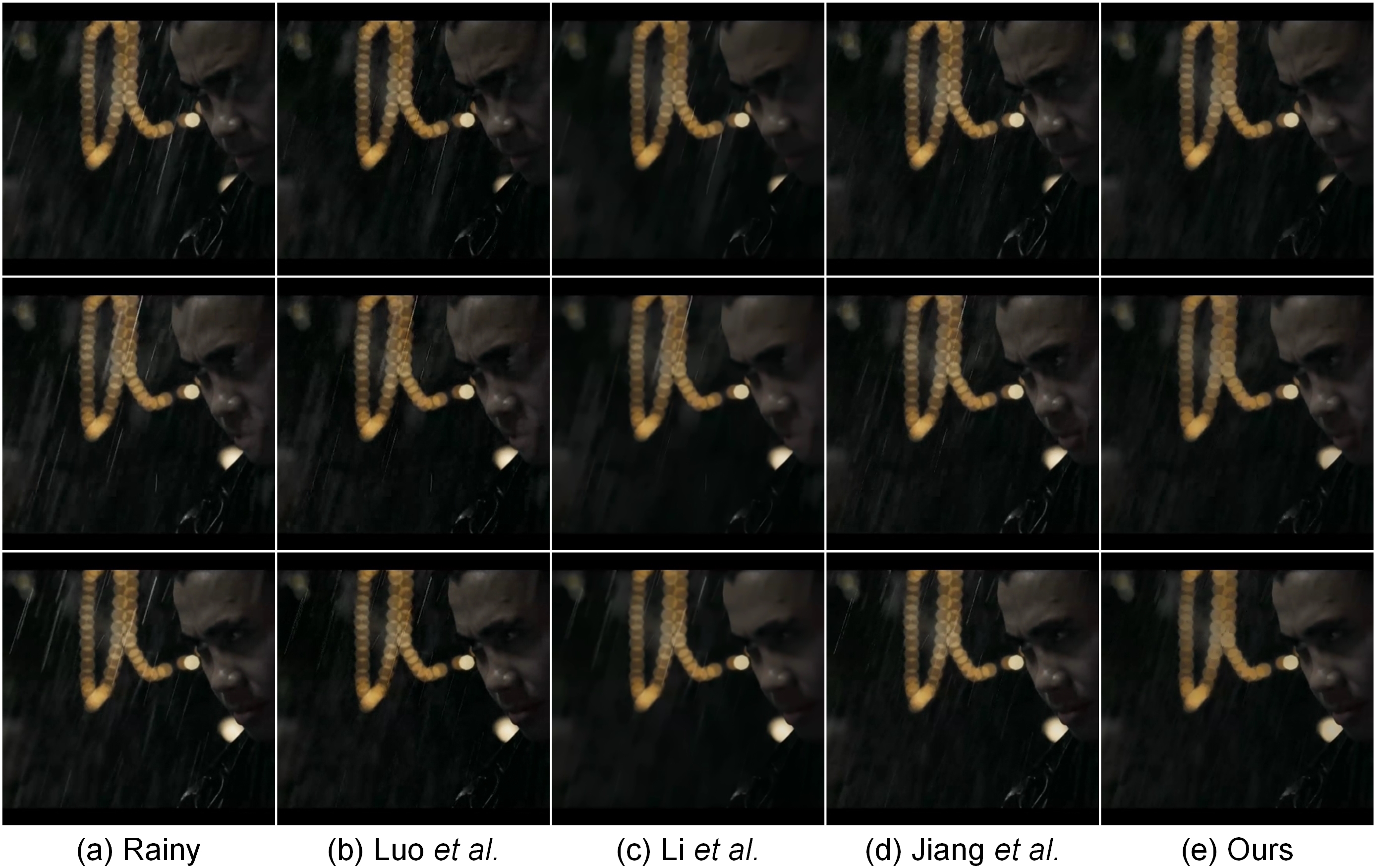
Fig. 3: Comparisons of deraining results on three frames extracted from the realistic “The Grandmaster” video. From left to right: (a) rainy images, restored images yielded by (b) Luo et al. [8], (c) Li et al. [9], (d) Jiang et al. [11] and (e) ours.

5 Conclusion

We proposed a directional regularized tensor modeling for video rain streaks removal in this work. The main contribution is the assumption that all rain streaks fall in an approximately similar arbitrary direction. Experiments show that the proposed method can effectively remove rain streaks while preserving fine details. It is worth pointing out that our method suffers mainly from two limitations: (1) high computational complexity; (2) difficultly handling extremely heavy rain streaks. These issues are the focuses of our future work.

References

- [1] M. Roser and A. Geiger, “Video-based raindrop detection for improved image registration,” in Proc. IEEE ICCV Workshops, Kyoto, Japan, Sep. 2009, pp. 570-577.
- [2] S. Maji, A. C. Berg, and J. Malik, “Classification using intersection kernel support vector machines is efficient,” in Proc. IEEE CVPR, Anchorage, AK, USA,Jun. 2008, pp. 1-8.
- [3] M. S. Shehata, J. Cai, W. M. Badawy, T. W. Burr, M. S. Pervez, R. J. Johannesson, and A. Radmanesh, “Video-based automatic incident detection for smart roads: The outdoor environmental challenges regarding false alarms,” IEEE Trans. Intell. Transp. Syst., vol. 9, no. 2, pp. 349-359, Jun. 2008.
- [4] K. Garg and S. K. Nayar, “Vision and rain,” Int. J. Comput. Vision, vol. 75, no. 1, pp. 3-27, Oct. 2007
- [5] D. Comaniciu, V. Ramesh, and P. Meer, “Kernel-based object tracking,” IEEE Trans. Pattern Anal. Mach. Intell., vol. 25, no. 5, pp. 564-577, May 2003.
- [6] K. Garg and S. K. Nayar, “Detection and removal of rain from videos,” in Proc. IEEE CVPR, Washington, DC, USA, Jun. 2004, pp. 1-8.
- [7] L. W. Kang, C. W. Lin, and Y. H. Fu, “Automatic single-image-based rain streaks removal via image decomposition,” IEEE Trans. Image Process., vol. 21, no. 4, pp. 1742-1755, Apr. 2012.
- [8] Y. Luo, Y. Xu, and H. Ji, “Removing rain from a single image via discriminative sparse coding,” in Proc. IEEE ICCV, Santiago, Chile, Dec. 2015, pp. 3397-3405.
- [9] Y. Li, R. T. Tan, X. Guo, J. Lu, and M. S. Brown, “Rain streak removal using layer priors,” in Proc. IEEE CVPR, Las Vegas, NV, USA, Jun. 2016, pp. 2736-2744.
- [10] J. H. Kim, J. Y. Sim, and C. S. Kim, “Video deraining and desnowing using temporal correlation and low-rank matrix completion,” IEEE Trans. Image Process., vol. 24, no. 9, pp. 2658-2670, Sep. 2015.
- [11] T. X. Jiang, T. Z. Huang, X. L. Zhao, L. J. Deng, and Y. Wang, “A novel tensor-based video rain streaks removal approach via utilizing discriminatively intrinsic priors,” in Proc. IEEE CVPR, Honolulu, HI, USA, Jul. 2017, pp. 2818-2827.
- [12] W. Wei, L. Yi, Q. Xie, Q. Zhao, D. Meng, and Z. Xu, “Should we encode rain streaks in video as deterministic or stochastic,” in Proc. IEEE ICCV, Venice, Italy, Oct. 2017, pp. 2516-2525.
- [13] A. K. Tripathi and S. Mukhopadhyay, “Removal of rain from videos: A review,” Signal, Image and Video Processing, vol. 8, no. 8, pp. 1421-1430, Nov. 2014.
- [14] W. Yang, R. T. Tan, J. Feng, J. Liu, Z. Guo, and S. Yan, “Deep joint rain detection and removal from a single image,” in Proc. IEEE CVPR, Honolulu, HI, USA, Jul. 2017, pp. 1357-1366.
- [15] X. Fu, J. Huang, X. Ding, Y. Liao, and J. Paisley, “Clearing the skies: A deep network architecture for single-image rain removal,” IEEE Trans. Image Process., vol. 26, no. 6, pp. 2944-2956, Jun. 2017.
- [16] J. Liu, W. Yang, S. Yang, and Z. Guo, “Erase or fill? Deep joint recurrent rain removal and reconstruction in videos,” in Proc. IEEE CVPR, Salt Lake City, UT, USA, Jun. 2018, pp. 3233-3242.
- [17] J. Liu, W. Yang, S. Yang, and Z. Guo, “D3R-Net: Dynamic routing residue recurrent network for video rain removal,” IEEE Trans. Image Process., vol. 28, no. 2, pp. 699-712, Feb. 2019.
- [18] R. Liu, Z. Jiang, L. Ma, X. Fan, H. Li, and Z. Luo, “Deep layer prior optimization for single image rain streaks removal,” in Proc. IEEE ICASSP, Calgary, AB, Canada, Apr. 2018, pp. 1408-1412.
- [19] R. W. Liu, L. Shi, W. Huang, J. Xu, S. C. H. Yu, and D. Wang, “Generalized total variation-based MRI Rician denoising model with spatially adaptive regularization parameters,” Magn. Reson. Imaging, vol. 32, no. 6, pp. 702-720, Jun. 2014.
- [20] Y. L. Chen and C. T. Hsu, “A generalized low-rank appearance model for spatio-temporally correlated rain streaks,” in Proc. IEEE ICCV, Sydney, NSW, Australia, Dec. 2013, pp. 1968-1975.
- [21] W. Ren, J. Tian, Z. Han, A. Chan, and Y. Tang, “Video desnowing and deraining based on matrix decomposition,” in Proc. IEEE CVPR, Honolulu, HI, USA, Jul. 2017, pp. 4210-4219.
- [22] S. Boyd, N. Parikh, E. Chu, B. Peleato, and J. Eckstein, “Distributed optimization and statistical learning via the alternating direction method of multipliers,” Found. Trends Mach. Learn., vol. 3, no. 1, pp. 1-122, 2011.
- [23] R. D. Kongskov and Y. Dong, “Directional total generalized variation regularization for impulse noise removal,” in Proc. SSVM, Graz, Austria, Jun. 2017, pp. 221-231.
- [24] İ. Bayram and M. E. Kamasak, “Directional total variation,” IEEE Signal Process Lett., vol. 19, no. 12, pp. 781-784, Dec. 2012.