The application of co-integration theory in ensemble pulsar timescale algorithm

Abstract

Employing multiple pulsars and using an appropriate algorithm to establish ensemble pulsar timescale can reduce the influences of various noises on the long-term stability of pulsar timescale, compared to a single pulsar. However, due to the low timing precision and the significant red noises of some pulsars, their participation in the construction of ensemble pulsar timescale is often limited. Inspired by the principle of solving non-stationary sequence modeling using co-integration theory, we puts forward an algorithm based on the co-integration theory to establish ensemble pulsar timescale. It is found that this algorithm can effectively suppress some noise sources if a co-integration relationship between different pulsar data exist. Different from the classical weighted average algorithm, the co-integration method provides the chances of the pulsar with significant red noises to attend the establishment of ensemble pulsar timescale. Based on the data from the North American Nanohertz Observatory for Gravitational Waves, we found that the co-integration algorithm can successfully reduce several timing noises and improve the long-term stability of the ensemble pulsar timescale.

1 Introduction

Pulsar timing is an effective tool in studying astrophysics and fundamental physics. These include tests of gravitation, precision constraints of general relativity, and especially using arrays of pulsars as detectors of low-frequency gravitational wave (Zhu et al. 2015; Will 2014; Arzoumanian et al. 2015a). The basis of pulsar timing is the high-precision timing model, accomplished by the determination of a series model parameters, such as the spin parameters, astrometric parameters, binary orbit parameters and so on. The errors of the model parameters will affect the timing precision in different ways(Tong et al. 2017). At present, millisecond pulsars (MSPs) have higher stability of rotation and are more widely used in the study of pulsar time scale (Splaver 2004; Verbiest et al. 2009). For example, G. Hobbs (Hobbs et al. 2012) obtained a preliminary pulsar time scale based on Parkes Pulsar Timing Array including 19 millisecond pulsars observed by Parkes radio telescope. It was shown that pulsar timing array allows investigation of “global” phenomena, such as a background of gravitational waves or instabilities in atomic time scales that produce correlated timing residuals in the pulsars of the array. However, there are various physical processes that might be responsible for the accuracy of pulsar time scale, timing noise is still not fully understood, but usually refers to unexplained low-frequency features in the timing residuals of pulsars. In the presence of red timing noise, W. Coles (Coles et al. 2011) adopted a transformation based on the Cholesky decomposition of the covariance matrix that whitens both the residuals and the timing model, which has sufficient accuracy to optimize the pulsar timing analysis. In addition, using data from multiple pulsars, it is possible to obtain an average pulsar time scale that has a stability better than those derived from individual pulsar data(Petit et al. 1993; Rodin 2008; Zhong & Yang 2007; Hobbs et al. 2010).

The purpose of using multiple pulsars data is to suppress the timing noise intensity of individual pulsar. It will open up a new window to improve the accuracy and long-term stability of pulsar timescale by establishing ensemble pulsar timescale (EPT). However, similar to the establishment of atomic time scale (AT) the accuracy and long-term stability of EPT depend significantly on the information of timing residuals of pulsars data involved. The lower the timing noise is, the better the result of EPT will be obtained, which often limits the participation of a large number of pulsars with significant timing noise. Based on the timing clock model analysis, any clock model can be regarded as the connection between the regression model and time series variables. Whether establishing a well pulsar timescale or make its forecast, the clock difference series should be stationary. Only in this way can we ensure that some statistic parameters in the selection and examination of the model, such as determinable coefficient $R^{2}$ and $T$ statistics, have standard normal distribution, and therefore, the statistics are reliable. Otherwise, all of the above inferences can easily produce a spurious regression.

In the economics fields, in order to avoid spurious regression of non-stationary series, Engle and Granger proposed the co-integration theory that provided another way for the modeling of non-stationary series(Engle & Granger 1987). For example, although some economic variables themselves are non-stationary series, but linear combination of them is likely to be stationary. This combining process is known as co-integration equation, and it can explain the long-term equilibrium relationship between different variables. In principle, the pulsars with significant timing noise show the non-stationary characteristics of timing residuals, if the linear combination of pulsars timing residuals is stationary series, they are also co-integration. According to the above ideas, an algorithm based on co-integration theory to establish EPT is proposed in this paper, which mainly use the pulsars with significant timing noise, and the results show that the algorithm can successfully reduce several timing noises and improve significantly the long-term frequency stability of EPT. Co-integration is a powerful method, because it not only allows us to characterize the equilibrium relationship between two or more no-stationary series, but also will provide a better guidance in studying the establishment of EPT in future.

2 Co-integration and method

In the process of regression analysis for most non-stationary time series, the difference method is usually used to eliminate the non-stationary trend term in the series, so that the series can be modeled after it is stationary. However, the series themselves after difference calculation often are limited the scope of the problem discussed and make the reconstructed model difficult to explain. The co-integration theory has greatly improved the difficulty of non-stationary series in modeling. The co-integration theory is proposed for integration. A series with no deterministic component which has a stationary, invertible, ARMA representation after difference $d$ times, is said to be integrated of order $d$, denoted $Y_{t}\thicksim I(d)$. Obviously, for $d=0$, $Y_{t}$ will be stationary.

The co-integration theory can be understood as that there may be a long-term equilibrium relationship between several time series with the same order of integration, and one kind of linear combination of them has a lower order of integration. To formalize these ideas, the following definition adopted from Engle and Granger is introduced: (i) if all components of $Y_{t}$ are $I(d)$; (ii) there exists a vector $\alpha$ ($\neq$ 0) so that $\alpha^{{}^{\prime}}Y_{t}\thicksim I(d-b)$, $d\geq b\geq 0$. The components of the vector $Y_{t}$ are said to be co-integrated of order d, b, denoted $Y_{t}\thicksim CI(d-b)$, and the vector $\alpha$ is called the co-integrating vector.

In general, there are two main methods to examine the co-integration, including Engle-Granger (EG) two-step method and Johansen-Juselius(JJ) multivariate maximum likelihood method (Engle & Granger 1987; Johansen 1995). The major difference between the above methods is that the EG two-step method adopts solving linear equation technique, while the JJ test uses the multivariate equation technique. In this paper, EG method is adopted to assess the null hypothesis of no co-integration among the time series in $Y_{t}$. Detailed test steps can be seen in Ref.(Engle & Granger 1987).

3 EPT algorithm based on co-integration theory

In pulsar timing, the timing residuals are the differences between the observed times of arrival (TOAs) and the ones predicted by the timing model, i.e., the difference between two time scales, AT and PT. Here, AT and PT stand for the atomic time scale and pulsar time scale, respectively. However, in the practical data processing, the AT recorded the TOAs should be transferred to Barycentric coordinate time(TCB), and PT is predicted at Solar system barycenter (SSB) by the pulsar timing model. Hence, for a given pulsar i, the residuals are denoted as:

$$Res_{i}=AT-PT_{i}\,,$$ (1)

where $Res_{i}$ is timing residuals; $AT$ is reference atomic time; $PT_{i}$ is pulsar time for a given pulsar i. The EPT (Petit & Tavella 1996) established by multiple pulsars (i=1, 2 $\cdots$, n) can be defined as:

$$AT-EPT=\sum\limits_{i=1}^{n}\omega_{i}(AT-PT_{i}),,$$ (2)

where $\omega_{i}$ is the relative weight assigned to pulsar i. Because we adopted EG test to analyze the pulsar data in this paper, hence, assume for two known pulsars whose timing residuals are $Res_{i}\thicksim I(1)$, and they are co-integrated, the co-integrated regression equation of both timing residuals can be expressed as:

$$Res_{1}=\alpha+\beta Res_{2}+\hat{\varepsilon}\,,$$ (3)

where $\alpha$ and $\beta$ represent regression coefficients; $\hat{\varepsilon}$ is the model residuals, and ,$\hat{\varepsilon}\thicksim I(0)$. According to formula (1)–(3) we obtain

$$\left\{\begin{array}[]{lr}\omega_{1}=\frac{1}{1-\beta},&\\ \omega_{2}=\frac{-\beta}{1-\beta},&\\ Res_{ept}=\frac{\hat{\varepsilon}+\alpha}{1-\beta}.&\end{array}\right.$$ (4)

where $Res_{\rm{ept}}$ represents the timing residuals of EPT, it can be regarded as a transformation from $\hat{\varepsilon}$ by shift factor $\alpha$ and scale factor $(1-\beta)$, and both $\alpha$ and $(1-\beta)$ are constant coefficients, which will not affect the order of integration, so, $Res_{\rm{ept}}\thicksim I(0)$.

4 Observational data

4.1 NANOGrav timing observations

We used pulsars timing data from the NANOGrav nine-year data set described in Arzoumanian et al.(hereafter NG9, Arzoumanian et al. 2015b) for our analysis. NG9 contains 37 MSPs observed at the Green Bank Telescop (GBT) and Arecibo Observatory (AO). Each telescope contains two generations of backends, with more recent backends processing up to an order of magnitude larger bandwidth for improving pulse sensitivity. Polarization calibration and RFI excision algorithms were applied to the raw data profiles using the PSRCHIVE (Hotan et al. 2004; van Straten et al. 2012) software package when pulse profiles were folded and de-dispersed using an initial timing model. After calibration, known RFI signal were excised, the final pulse profiles used to generate TOAs were fully time averaged with some frequency averaging to build pulse signal-to-noise ratio (S/N). See NG9 for more detail on the data processing. Because the purpose of this article is improve its long-term frequency stability of EPT consisting mostly pulsars with significant timing noise, and the stability of pulsar timescale is related to the timing span. So, in this paper, the requirement of selecting pulsars from NG9 includes that both the sampling time span is longer than 8 years, and detect obvious evidence for excess at low frequency, or “red” timing noise in timing residuals of the pulsars. We selected 7 pulsars that met these criteria, see the basic parameters of the selected 7 pulsars in Table 1.

Table 1: Basic Parameter of 7 Pulsars

Pulsar name	$P$ (ms)	Number of TOAs	RMS ($\mu$s)	Span (year)
J0030+0451	4.87	2468	0.723	8.8
J0613-0200	3.06	7651	0.592	8.6
J1012+5307	5.26	11995	1.197	9.2
J1643-1224	4.62	7119	2.057	9.0
B1855+09	5.36	4071	1.339	8.9
J1910+1256	4.98	2690	1.449	8.8
B1937+21	1.56	9966	1.549	9.1

4.2 Data preprocessing

NG9 contained all TOAs and timing solutions for 37 pulsars. Each pulsar was observed at each epoch with at least two receivers. At GBT, the 820 and 1400 MHz bands were used, and at AO, the 430 and 1400 MHz or 1400 and 2300 MHz band were used. We note that frequency-dependent profile shape changes across the entire observing band can be significant for some sources over the full band(Pennucci et al. 2014), and we wish to maintain homogeneity of the inferred timing data of our pulsars, we analyze timing residuals with 1400 MHz only. In addition pulsar B1937+21 just contain data from GBT. We use the unit root test with significance level 0.01 to analyze residual datas of 7 pulsars, the results show that they all seem to be stationary, Res$\thicksim$I(0). It may be due to mostly MSPs in NG9 have higher stability of rotation, the dispersion of timing residuals are dominated by white noise, or red noise is drowned out by white one within shorter observation span. Hence, selecting pulsar data with significant red noise and further reducing the white noise intensity in the timing residuals in some way that can make the processed data meet the condition of non-stationary, Res$\thicksim$I(1), which is equivalent to just retaining the red noise component in the original data. Besides, pulsars timing observation are usually irregular and whose sampling rate are much lower than that atomic clock comparison. Hence, a simple method will be adopted to reduce the intensity of the white noise and make the two columns of data involved in the co-integration test correspond to each other.

For long-term pulsar timing studies it becomes useful to visually inspect timing residuals that have been averaged in order to look for long term trends or biases. The following details of data preprocessing will be illustrated with one pulsar, i.e., J1937+21: Firstly, we construct daily averaged residuals, each residual value is equal to the average of all raw residuals within one day. This process is similar to comparing pulsar time with atomic clock once a day. Subsequently, the data are linear interpolated and sampled at intervals of about 15 days to obtain equally distributed data. The purpose of the above two-step is to reduce the white noise intensity and helpful further analysis whether the low-frequency noise in residuals for different pulsars have a co-integration relationship with each other. Other methods to discuss strictly the reduction of white noise intensity will be given in future work. The original timing residual distribution vs. two-step preprocessing residual data are shown in Figure 1. Similarly, other six known pulsars timing residuals are also regularly processed.

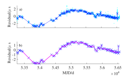
Figure 1: The raw timing residuals vs. two-step preprocessing residuals for pulsar B1937+21 (the cyan and blue represent the raw residuals vs. the averaged residuals in graph a, and blue and magenta stand for the averaged residuals vs. linear interpolation residuals in graph b).

5 Results and analysis

According to the mathematical model of the co-integration theory in sect. 3, it is necessary to examine integrated order of time series to determine whether there are co-integrated relationship. In this paper, EG method was adopted to examine timing residuals of all pulsars after preprocessed data, we found that pulsars B1855+09, B1937+21, J0030+0451 and J1910+1256 were integrated of order 1, denoted as $I(1)$, and for others were $I(0)$. These results may be due to the intensity of red noise in residuals of pulsars J0613-0200, J1012+5307 and J1643-1224 are relatively weak, after data preprocessing timing residuals still show some “quasi-stationary” features. In order to search for pulsars with co-integration relationship by using EG two-step method strictly, we only make further analysis on pulsars B1855+09, B1937+21, J0030+0451 and J1910+1256.

The timing residuals of pulsars B1855+09, B1937+21, J0030+0451 and J1910+1256 are shown in Figure 2, and the histograms of residuals distribution can be seen in Figure 3, respectively. In Figure 2, the timing residuals distributions of all pulsars show obvious irregular low-frequency trend terms, and histograms of residuals distribution are significantly different from the normal distribution in Figure 3. All of these indicate that the timing residuals for four known pulsars have a common feature of instability, which is consistent with the case where the integrated order of residuals are denoted as $I(1)$. In addition, by comparing the residual distributions, the standard deviations of the residuals, all show that there are significant differences for pulsar data each other, these differences are not only shown in the trend term of residuals distribution, but also in the shape of fitting curve. These are related to the fact that every pulsar data is affected by different sources of noise.

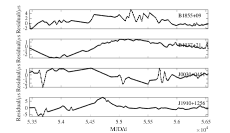
Figure 2: The timing residuals for four known pulsars B1855+09, B1937+21, J0030+0451 and J1910+1256, respectively.

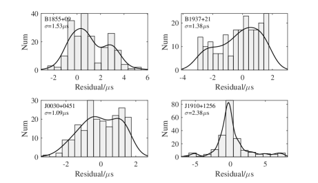
Figure 3: The histograms of timing residual distributions for four known pulsars B1855+09, B1937+21, J0030+045 and J1910+1256, respectively. The solid line is the fitting curve for each residual distribution. The value of standard deviations ($\sigma$) for four residual distributions are also given

Next, according to formula (3) in sect 3, we had further to examine the linear combination for residuals from two random pulsars (for example pulsars A and B) with denoted $I(1)$, if $\hat{\varepsilon}$ is integrated of order 0, then pulsars A and B are co-integrated. We found that only linear combination of pulsars B1937+21 and J0030+0451 had met the condition that the $\hat{\varepsilon}$ is denoted as $I(0)$. So it indicates that the Pulsars B1937+21 and J0030+0451 are co-integrated. The timing residuals of the EPT established by the pulsars B1937+21 and J0030+0451 can be obtained according to the formula (4) in sect 3 and marked as $\rm{EPT_{c}}$. In order to obtain the degree of stability of residuals, first of all, we compared both residual distributions and residual histograms for pulsars B1937+21, J0030+0451 and $\rm{EPT_{c}}$ in Figure 4 and 5. In Figure 4, we can see that the amplitude fluctuation of residuals of pulsars B1937+0451 and J0030+0451 are stronger and have obvious low-frequency freatures, but the residuals for $\rm{EPT_{c}}$ are characterized by normalization, simplicity, significant reduction of non-stationary process, etc. The range of residuals amplitude variation for pulsars B1937+21, J0030+0451 and $\rm{EPT_{c}}$ are (-2.91,+1.74) $\mu$s, (-3.03,+1.66) $\mu$s and (-2.47,+1.19) $\mu$s, respectively. The standard deviation for $\rm{EPT_{c}}$ is smallest. In addition, the shape of fitting curve for $\rm{EPT_{c}}$ in Figure 5 is also closer to normal distribution than that those of pulsars B1855+09 and J0030+0451. The above contents all indicate that the degree of stability of $\rm{EPT_{c}}$ has been greatly improved.

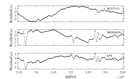
Figure 4: The timing residuals for two known pulsars B1937+21, J0030+0451 and for ensemble pulsar timescale $\rm{EPT_{c}}$, respectively.

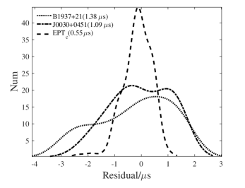
Figure 5: The fitting curves of timing residual distributions for two known pulsars (dotted line for B1937+21 and dash-dot line for J0030+0451) and for ensemble pulsar timescale (dashed line for $\rm{EPT_{c}}$), respectively. The value of standard deviation for three residual distributions are also given in brackets.

5.1 Variance analysis

The dispersion of pulsar timing residuals can be divided into white and red noise. White noise mainly comes from the random errors in the process of timing observation, while red noise is a kind of signal having strong intensity at lower frequencies, giving it a power-law spectral density. We can define the dispersion of residual as $\sigma_{\rm RMS}$, while white noise is denoted $\sigma_{\rm W}$ and red noise is denoted $\sigma_{\rm TN}$(Yang et al. 2014; Gao et al. 2018). In theory, their relations are following as:

$${\sigma_{\rm RMS}}^{2}={\sigma_{\rm W}}^{2}+{\sigma_{\rm TN}}^{2}\,.$$ (5)

where if the ratio of $\sigma_{\rm RMS}$ to $\sigma_{\rm W}$ is close to 1, it indicates that the dispersion of residual is mainly affected by white noise, and the data is stationary. If the value of $\sigma_{\rm RMS}/\sigma_{\rm W}$ is much higher than 1, it indicates that there is a significant red noise component within the timing residuals. Generally, the effect of red noise on dispersion of residual changes with increasing of observing span, to reflect this change, the Ref.(Gao et al. 2018; Lam et al. 2017) used variance increment to show the important contribution of red noise to residual fluctuation. Considering that the dimension of standard deviation is consistent with the magnitude of data, it is more obvious when describing data dispersion, and the variance and standard deviation can be easily converted to each other, as defined by Gao(Gao et al. 2018), the standard deviation increment is defined as follows:

$$\Delta\sigma(\tau)=\langle Var(X(t+\tau))^{1/2}-Var(X(t))^{1/2}\rangle\,,$$ (6)

where $t$ stands for timing span, $Var(X(t))$ represents the variance of the data in $t$, and $\tau$ is the increment of timing span. In theory, for data with significant system fluctuations, the standard deviation increment will change with the increase of $\tau$. In this paper, we take the pulsar B1937+21 as an example to illustrate how to choose the values of the parameters $t$ and $\tau$. After data preprocessing, there are 206 points of residuals for pulsar B1937+21 in 8.4 years, the interval between two points is approximately 15 days. To take $t$ as the interval span of adjacent 10 points, for $\tau$=0, 10, 20, $\cdots$, add 10 points interval span one by one. Meanwhile, in order to avoid introducing statistical error, the standard deviation increment in (6) is averaged. The timing span is divided into two segments at least, so the maximum span of $\tau$ is nearly half of 8.4 years. Similarly, pulsar J0030+0451 and $\rm{EPT_{c}}$ are same processed, The relations between standard deviation increment and timing span for 3 pulsars are shown in Figure 6.

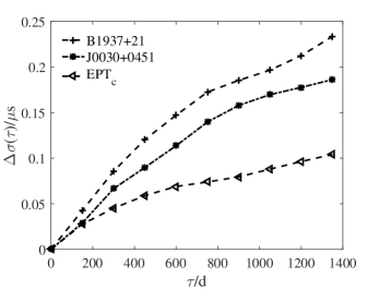
Figure 6: The standard deviation increment of timing residuals vs. timing span for two known pulsars (plus sign for B1937+21 and asterisk for J0030+0451) and for ensemble pulsar timescale (left-pointing triangle for $\rm{EPT_{c}}$), respectively.

As it show that in Figure 6, the values of $\Delta\sigma(\tau)$ for pulsars B1937+21 and J0030+0451 increase rapidly with the change of $\tau$, while the $\Delta\sigma(\tau)$ for $\rm{EPT_{c}}$ changes slowly. This is because the red noise in the residual of pulsars B1937+21 and J0030+0451 are obvious, along the timing span increase, strong red noise becomes an important factor for the dispersion of the residual of pulsar. This is consistent with the fact that the integrated order of two pulsars are 1. It can also be explained that the linear combination of pulsar residuals which are co-integration is stationary series by $\rm{EPT_{c}}$.

5.2 $\sigma_{z}(\tau)$ methods

Using the exceptional rotational stability of millisecond pulsars to generate a time scale need a reliable statistical measure for studying the physics of pulsar rotation and comparing pulsar stabilities with those of terrestrial clocks. Clock data are commonly analyzed using a statistic called $\sigma_{y}(\tau)$, the square root of the “Allan variance” (Allan 1966), which can be computed from second differences of a table of clock offset measurements. $\sigma_{y}(\tau)$ is ideally suited for analyzing atomic timescale which have very small frequency drift rates. However, for most pulsars timing data, the lowest-order deviations is related to $third$ differences, which is remaining in a pulsar timing series after the phase, frequency, spin-down rate, and astrometric parameters have been determined by comparison with terrestrial time, and their effects removed. Following Taylor (Taylor 1991), the statistic $\sigma_{z}(\tau)$ defined in terms of third-order polynomials fitted to sequences of measured time offsets is suggested for studying the pulsar timing data. Since it is more sensitive to redder noise than other commonly used measures, and is suited for comparing pulsar stabilities with those of other time scales. In this paper, we use an improved $\sigma_{z}(\tau)$ proposed by Matsakis (Matsakis et al. 1997), which is a good statistic for the analysis of low-frequency-dominated red noise of pulsar timing residuals. To find $\sigma_{z}(\tau)$, divide the data into subsequences, and fit the cubic function to the data in each subsequence by minimizing the weighted sum of squared differences

$$R^{2}=\sum\limits_{i=1}^{N_{m}}\left[x(t_{i})-\frac{X(t_{i})}{\sigma_{i}}\right]^{2}=min\,,$$ (7)

Then set

$$\sigma_{z}(\tau)=\frac{\tau^{2}}{2\sqrt{5}}\langle c_{3}^{2}\rangle^{1/2}\,.$$ (8)

where angle brackets denote averaging over the subsequences, weighted by the inverse squares of the formal errors in $c_{3}$. The detailed recipe for the computation of $\sigma_{z}(\tau)$ can be seen in Ref.(Matsakis et al. 1997).

In Figure 7, we present values of $\sigma_{z}(\tau)$ for all pulsars B1937+0451, J0030+0451 and $\rm{EPT_{c}}$, defined as the weighted root-mean-square of the coefficients of the cubic terms fitted over intervals of length $\tau$. For comparison, another EPT calculated by traditional classical weighted average algorithm is given in Figure 7, the weights $\omega_{i}$ are inversely proportional to the variance of two pulsars 1937+21 and J0030+0451, respectively. Because $\sigma_{z}^{2}(\tau)$ can be easy to describe by a power law, if the white noise is dominate in the time series, the slope of the log-log graph is close to -1.5, for all four time series show that at least up to intervals $\tau$ of several years, as expected for residuals dominated by uncorrelated measurement errors. On the contrary, when the red noise is dominant, the tail of the curve will gradually become an upward trend, which is represented as the influence of low-frequency noise on the frequency stability. For both pulsars B1937+21 and J0030+0451, the curves show a tail upward trend, while the curves of both $\rm{EPT_{c}}$ and EPT show a downward trend as a whole, it indicates that the timing residuals for two pulsars B1937+21 and J0030+0451 are dominated by low-frequency noise believed to be intrinsic to the pulsars. It is note that the stability of pulsar time scale for pulsar J0030+0451 at $\log\tau\thicksim$0.6 is more stable than $\rm{EPT_{c}}$. This anomaly should be induced by the increasing errors of $\sigma_{z}$ for larger intervals of length $\tau$ because of the decreasing number of sequences .

The long-term frequency stability level plays an important role in the study of pulsar time scales, Figure 7 shows that the value of $\sigma_{z}(\tau)$ for two pulsars B1937+0451 and J0030+0451 and for ensemble pulsar timescale calculated by different algorithm $\rm{EPT_{c}}$ and EPT on the span 8.4 years are 10^-13.70, 10^-13.61, 10^-15.20 and 10^14.12, respectively. The long-term frequency stability of $\rm{EPT_{c}}$ is nearly one order of magnitude higher than those of the other two pulsars B1937+0451 and J0030+0451. In addition, one can note that the stability of $\rm{EPT_{c}}$ is better than EPT as a whole in Figure 7. The above analysis indicates that the long-term frequency stability level of pulsar can be significantly improved within a limited observation span when combining the pulsars data with co-integration relation to establish EPT. One thing to keep in mind is that these stabilities of pulsars in Figure 7 are not further compared with both other pulsars data with weak red noise and atomic timescale at different stations, this is because there are many factors influencing the stabilities of different timescale. In this paper, we only show that the method to establish EPT based on combining the pulsars data with the co-integration relation is reliable and feasible, further research will be carried out in the follow-up work.

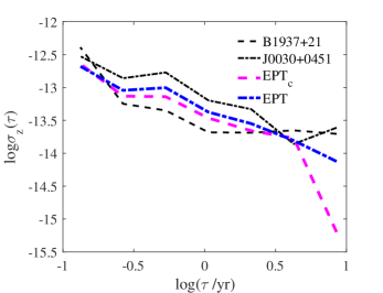
Figure 7: Stability of pulsar time scale for two known pulsars (dashed line for B1937+21 and dash-dot line for J0030+0451) and for ensemble pulsar timescale calculated by different algorithm (magenta dashed line for $\rm{EPT_{c}}$ and blue dash-dot line for EPT), respectively.

6 Discussion and Conclusions

It should be noted that it is necessary to satisfy a strict constraint condition to establish EPT based on the co-integration theory: the timing residuals of pulsars are co-integration. The combination of timing residuals with co-integration relation can only reduce the number of integrated order, and in this way it can obviously reduce the timing noise intensity of EPT and improve its long-term frequency stability. According to this constraint condition, it means that the following problems may be encountered in practical application: (1) In the short span, the red noise in residuals of millisecond pulsars are not dominant or can not be measured, residuals data show “quasi-stationary” characteristics , so it will limit the methods in application pulsars data. (2) At present, the low-frequency timing noise of most pulsars data are irregular, which means that the co-integration relation between pulsars may be damaged by the increase or decrease of the data span, it may lead to segmented co-integration. In addition, we only use the EG(Engle & Granger 1987) two-step test to discuss and establish EPT algorithm based on two pulsars in this paper, if the data of multiple pulsars are regarded as multivariate variables, and the co-integration relation between them is tested by using JJ(Johansen 1995) methods , the application of co-integration theory in the algorithm of EPT can be further extended.

Based on the co-integration theory, an algorithm to establish EPT by using pulsars data with significant timing noise is proposed in this paper, this algorithm can successfully reduce several timing noises and improve the long-term stability of pulsar timescale. Compared to the optimal weighting method (Rodin 2008) and the global fitting method (Hobbs et al. 2012), our co-integration method is similar to the traditional classical weighted average method but with a new way of choosing weights. However, different from the traditional classical weighted average algorithm , this algorithm can effectively suppress some noise sources if there is a co-integration relationship between different pulsar data, and provides the chances of the pulsar with significant red noises to attend the establishment of ensemble pulsar timescale.