On Constraining the Growth History of Massive Black Holes via Their Distribution on the Spin-Mass plane

Abstract

The spin distribution of massive black holes (MBHs) contains rich information on the MBH growth history. In this paper, we investigate the spin evolution of MBHs by assuming that each MBH experiences two-phase accretion, with an initial phase of coherent-accretion via either the standard thin disc or super-Eddington disc, followed by a chaotic-accretion phase composed of many episodes with different disc orientations. If the chaotic-phase is significant to the growth of an MBH, the MBH spin quickly reaches the maximum value because of the initial coherent-accretion, then changes to a quasi-equilibrium state and fluctuates around a value mainly determined by the mean ratio of the disc to the MBH mass ($M_{\bullet}$) in the chaotic-accretion episodes, and further declines due to late chaotic-accretion if $M_{\bullet}\gtrsim(1-3)\times 10^{8}M_{\odot}$. The turning point to this decline is determined by the equality of the disc warp radius and disc size. By matching the currently available spin measurements with mock samples generated from the two-phase model(s) on the spin-mass plane, we find that MBHs must experience significant chaotic-accretion phase with many episodes and the mass accreted in each episode is roughly 1-2 percent of $M_{\bullet}$ or less. MBHs with $M_{\bullet}\gtrsim 10^{8}M_{\odot}$ appear to have intermediate-to-high spins ($\sim 0.5-1$), while lighter MBHs have higher spins ($\gtrsim 0.8$). The best matches also infer that (1) the radiative efficiencies ($\eta$) of those active MBHs appear to slightly decrease with $M_{\bullet}$; however, the correlation between $\eta$ and $M_{\bullet}$, if any, is weak; (2) the mean radiative efficiency of active MBHs is $\left<\eta\right>\sim 0.09-0.15$, consistent with the global constraints.

1. Introduction

Observations have shown that massive black holes (MBHs) ubiquitously exist in the centers of ellipticals and spiral bulges (e.g., Kormendy & Richstone, 1995; Magorrian et al., 1998; Kormendy & Ho, 2013). These MBHs are thought to be completely described by the Kerr metric with only two physical parameters, i.e., mass $M_{\bullet}$ and dimensionless spin parameter $a$. Measuring the masses and spins of these MBHs and obtaining their distributions are of great importance in revealing their formation and assembly histories.

The masses of MBHs in the centers of both nearby quiescent and active galaxies can be estimated with considerable accuracy by using the motion of gas and/or stars surrounding the MBHs (e.g., Macchetto et al., 1997; Gebhardt & Thomas, 2009; Peterson et al., 2004). Tight correlations have been found between the MBH mass and properties of their host galaxies (e.g., stellar velocity dispersions, bulge luminosities or masses, etc.) in the local universe (e.g., Ferrarese et al., 2000; Gebhardt et al., 2000; Tremaine et al., 2002; Kormendy & Richstone, 1995; Magorrian et al., 1998; Gültekin et al., 2009; Kormendy & Ho, 2013; Saglia et al., 2016), which suggests that MBHs co-evolve with their host galaxies. It has also been shown that the mass growth of MBHs is dominated by accretion during the QSO/AGN phases by comparing the local MBH mass density with the accreted MBH mass density over the cosmic time (e.g., Yu & Tremaine, 2002; Marconi et al., 2004; Yu & Lu, 2004; Shankar et al., 2009) via the Sołtan (1982) argument.

The spins of active MBHs are much more difficult to measure. Currently it is widely agreed that they can be measured via the X-ray reflection spectroscopy based on the assumption that the accretion disc is geometrically thin and optically thick, and the inner disc boundary, i.e., the innermost stable circular orbit (ISCO), is solely determined by the MBH spin (Brenneman & Reynolds 2006; for a review of MBH spin measurements, see Brenneman 2013; Reynolds 2014). The most significant feature in the X-ray reflection spectrum is the relativistically broadened and skewed Fe K$\alpha$ line (e.g., Fabian et al., 1989; Laor, 1991), the profile of which provides a measure to the spin of the central MBH (e.g., Tanaka et al., 1995). However, X-ray spectroscopic observations of QSOs/AGNs with sufficiently high quality are very limited. Currently, there are only about two dozen MBHs that have relatively robust spin measurements, as summarized in Table 1 (see also Reynolds, 2014; Brenneman, 2013; Vasudevan et al., 2016). If ignoring the measurement errors, all MBHs in this sample have spins $a>0.4$, and about two thirds of them have $a>0.8$.

If an MBH merges with another MBH or accretes gaseous material, the spin of the MBH evolves. Mergers of two MBHs with comparable mass generally result in a spin value of $\sim 0.7-0.9$ (e.g., Gammie et al., 2004; Centrella et al., 2010; Lousto et al., 2010; Lehner & Pretorius, 2014), but may leave little long-term effect on the MBH spin evolution (King et al., 2008). However, the MBH spin may increase or decrease by accreting gaseous material, depending on the relative orientation of the accretion disc angular momentum with respect to the MBH spin (e.g., King & Pringle, 2006; Perego et al., 2009), although the MBH mass grows monotonically. Significant gas accretion plays a critical role in the evolution of MBH spin and may lead to a spin distribution over a large range (e.g., King et al. 2008; Volonteri et al. 2013; Dotti et al. 2013). It has been shown that an MBH may end up with an extremely high spin (close to 1) if the disc accretion has a preferred direction (hereafter coherent-accretion; e.g., Thorne 1974). However, the MBH may be spun down or up if the accretion is episodic with disc orientations randomly distributed in different episodes (hereafter chaotic accretion), and the MBH can be spun down to $a\sim 0$ even if the initial spin is close to $1$ simply because negative angular momentum injection by retrograde accretion is more effective than positive angular momentum injection by prograde accretion (e.g., Bardeen et al., 1972; Moderski et al., 1998). In principle, different accretion and assembly histories of MBHs may result in different spin distributions, and thus observationally determined spin distribution can be used to put constraints on the MBH accretion history (e.g., Dotti et al., 2013; Sesana et al., 2014; Li et al., 2015).

In this paper, we use the latest available spin measurements for more than two dozen MBHs to put constraints on the accretion history of MBHs and check whether chaotic accretion is important in growing MBHs and shaping the spin distribution. The paper is organized as follows. In Section 2, we describe the spin evolution for different accretion modes, including coherent super-Eddington accretion, coherent standard thin disc accretion, and chaotic standard thin disc accretion. We assume that MBHs experience an initial coherent-accretion phase with either a super-Eddington rate or a standard thin disc rate, followed by a chaotic-accretion phase with each episode via standard thin disc accretion. Assuming this two-phase accretion model, we use the currently available spin measurements to obtain constraints on the accretion history of MBHs in Section 3. Some discussions are given in Section 4, and conclusions are summarized in Section 5.

Table 1Summary of the published MBH spin measurements via X-ray reflection spectroscopy

Object name	Galaxy type	z	$\log\left(L_{\rm bol}/{\rm erg\,s^{-1}}\right)$	$M_{\bullet}(10^{6}M_{\sun})$	a	Mass/Spin Refs
1H 0419-577	—	0.1040	46.03	$\sim 340$	$>0.89$	ZW05/Wa13
1H 0707-495	—	0.0407	44.43	$\sim 2.3$	$>0.97$	ZW05/Zo10
3C 120	S0	0.0330	45.34	$55^{+31}_{-23}$	$>0.95$	Pe04/Lo13
Ark 120	Sb/pec	0.0327	44.91	$150\pm 19$	$0.64^{+0.19}_{-0.11}$	Pe04/Wa13
Ark 564	SB	0.0247	44.21	$\sim 1.1$	$0.96^{+0.01}_{-0.07}$	ZW05/Wa13
Fairall 9	Sc	0.0470	45.23	$255\pm 56$	$0.52^{+0.19}_{-0.15}$	Pe04/Lo12
H 1821+643	—	0.2970	47.30	$4500\pm 1500$	$>0.4$	Re14/Re14
IRAS 00521-7054	—	0.0689	—	—	$\geq 0.84$	—/Ta12
IRAS 13224-3809	—	0.0658	45.55	$\sim 6.3$	$>0.985$	GS12/Fa13
MCG 6-30-15	E/S0	0.0570	44.18	$2.9^{+1.8}_{-1.6}$	$>0.98$	Mc05/BR06
Mrk 1018	S0	0.0424	44.39	$\sim 141$	$0.58^{+0.36}_{-0.74}$	Be11/Wa13
Mrk 110	—	0.0353	44.71	$25.1\pm 6.1$	$0.96^{+0.03}_{-0.07}$	Pe04/Wa13
Mrk 335	S0a	0.0258	44.69	$14.2\pm 3.7$	$>0.91$	Pe04/Ga15
Mrk 359	pec	0.0174	43.55	$\sim 1.1$	$0.66^{+0.30}_{-0.54}$	ZW05/Wa13
Mrk 79	SBb	0.0222	44.57	$52.4\pm 14.4$	$0.7\pm 0.1$	Pe04/Ga11
Mrk 841	E	0.0364	45.64	$\sim 79$	$>0.52$	ZW05/Wa13
NGC 1365	SB(s)b	0.0055	43.48	$\sim 2$	$\geq 0.84$	Ri09/Ri13
NGC 3783	SB(r)ab	0.0097	44.41	$29.8\pm 5.4$	$\geq 0.98$	Pe04/Br11
NGC 4051	SAB(rs)bc	0.0023	43.56	$1.91\pm 0.78$	$>0.99$	Pe04/Pa12
NGC 4151	SAB(rs)ab	0.0033	43.73	$45.7^{+5.7}_{-4.7}$	$>0.9$	Be06/Ke15
NGC 5506	Sa	0.0062	$\sim 44$	$5.11^{+2.20}_{-1.18}$	$0.93\pm 0.04$	Ni09/Su17
Q 2237+305	—	1.695	$\sim 45$	$1200\pm 1080$	$0.74^{+0.06}_{-0.03}$	Ass11/Rey14
RBS 1124	—	0.2080	45.53	$\sim 180$	$>0.97$	Mi10/Wa13
RXS J1131-1231	—	0.658	$\sim 45$	$\sim 200$	$0.87^{+0.08}_{-0.15}$	Sl12/Rei14
SDSS J094533.99+100950.1	—	1.66	46.79	$\sim 2700$	$0.8^{+0.2}_{-0.5}$	Cz11/Cz11
Swift J0501.9-3239	SB0/a(s)/pec	0.0124	44.11	$45\pm 15$	$\geq 0.92$	Ag14/Wa13
Swift J2127.4+5654	—	0.0144	44.53	$\sim 15$	$0.6\pm 0.2$	Ma08/Mi09
Ton S180	—	0.0620	45.30	$\sim 8.1$	$0.92^{+0.03}_{-0.11}$	ZW05/Wa13

2. Spin evolution of MBHs

2.1. Accretion history of MBHs

If a galaxy is rich in gas, once it experiences violent perturbations such as major mergers or disc instabilities, a large fraction of gas will be poured into the galactic center (e.g., Krolik, 1999), which naturally triggers disc accretion (either sub-Eddington or super-Eddington) onto the central MBH. With the consumption of gaseous material, the accretion process may be episodic afterwards due to infalling of single gas cloud, and in different episodes the disc angular momentum could be randomly oriented with respect to the MBH spin if there is no mechanism to make the gas cloud infall with a preferred direction.

As suggested by demographic studies of SDSS QSOs and X-ray AGNs (e.g., Shen et al., 2008; Schulze & Wisotzki, 2010; Suh et al., 2015), most QSOs and AGNs are accreting via sub-Eddington rate, i.e., $L_{\rm bol}/L_{\rm Edd}\sim 0.01-1$. Here $L_{{\rm bol}}$ is the bolometric luminosity and $L_{\rm Edd}=\frac{4\pi GM_{\bullet}m_{\rm p}c}{\sigma_{\rm T}}\simeq 1.3\times 10^{46}\left(\frac{M_{\bullet}}{10^{8}M_{\odot}}\right){\rm erg\,s^{-1}}$ is the Eddington luminosity, with $G$ the gravitational constant, $m_{\rm p}$ the proton mass, $c$ the speed of light and $\sigma_{\rm T}$ the Thomson cross section. With such a moderate accretion rate, the disc is radiatively efficient and can be described by the standard thin disc model (Shakura & Sunyaev, 1973; Novikov & Thorne, 1973). However, there are two lines of observations suggesting that MBHs may accrete material via super-Eddington rate in the early stage of its growth. First, MBHs with mass $>10^{9}M_{\odot}$ have already formed at redshift $z>6$ when the universe is less than $1$ Gyr old (e.g., Mortlock et al., 2011; Wu et al., 2015; Bañados et al., 2018). These observations raise a significant challenge to the growth theory for those MBHs since an MBH with mass $>10^{9}M_{\odot}$ cannot grow up from a small seed black hole (e.g., $<100M_{\odot}$) via the Eddington-limited accretion within a time period $<1$ Gyr. One popular solution to this is that those MBHs accrete via a super-Eddington rate, at least at the early stage (e.g., Li, 2012; Madau et al., 2014). Second, a number of nearby AGNs are recently found to be accreting via super-Eddington rate by adopting the MBH masses estimated from the reverberation mapping technique (e.g., Du et al., 2015). For such super-Eddington accretion flows, thick discs will be formed around the central MBHs (e.g., Abramowicz et al., 1988), as the emitted photons are trapped by the high density accretion flows and the discs cannot be cooled efficiently.

In addition, it has been shown that the net lifetime of QSOs is larger than $10^{7}-10^{8}$ yr (e.g., Yu & Lu, 2008; Shankar et al., 2009), while the period of a single accretion epoch could be as short as $10^{4}-10^{6}$ yr (e.g., Martini, 2004), which suggests the accretion processes may be episodic and the time duration for individual episode can be substantially shorter than the net lifetime. Recent observations also reveal a number of changing-look AGNs on timescale of $\sim 10$ yr, which are probably due to significant changes in the accretion rate (e.g., LaMassa et al., 2015; Ruan et al., 2016). These may also suggest that MBH accretion is episodic, especially at its later growth stage.

According to the above observational results, we assume a two-phase accretion model to describe the growth of MBHs. In the first phase, MBHs experience continuous and coherent accretion, during which the disc orientation maintains the same. In this phase, the accretion rate could be below or above the Eddington rate. After that, those MBHs undergo chaotic thin disc accretion, which contains many accretion episodes, and in each episode the disc angular momentum is arbitrarily oriented with respect to the MBH spin. We ignore the MBH change due to mechanisms in between any two adjacent accretion episodes.

We define normalized accretion rate as $\dot{m}=\dot{M}/\dot{M}_{\rm Edd}$, where $\dot{M}_{\rm Edd}\simeq 16\ L_{\rm Edd}/c^{2}$ (according to Madau et al. 2014) is the critical accretion rate for a non-rotating MBH whose accretion disc radiates at Eddington luminosity $L_{\rm Edd}$. The accretion is super-Eddington if $\dot{m}>1$.

2.2. Spin evolution due to coherent and chaotic accretion

Regardless of accretion patterns, if an MBH accretes with Eddington ratio $f_{\rm Edd}$ and radiative efficiency $\eta$, the MBH growth rate can be expressed as

$$\frac{{\rm d}M_{\bullet}}{{\rm d}t}=(1-\eta)\frac{f_{\rm Edd}}{\eta}\frac{M_{\bullet}}{t_{\rm Edd}},$$ (1)

where $t_{\rm Edd}\equiv M_{\bullet}c^{2}/L_{\rm Edd}\simeq 4.5\times 10^{8}$ yr is the Eddington timescale. The above equation is obtained by assuming that the kinetic energy loss is negligible and $\eta=1-E(R_{\rm in})$, where $E(R_{\rm in})$ is the specific energy at the inner disc boundary $R_{\rm in}$.

Generally, the initial disc angular momentum can be misaligned with the MBH spin, and the disc will suffer from warps due to the Lense-Thirring (LT) precession (Lense & Thirring, 1918). Since the LT precession frequency decreases with increasing radius ($\propto R^{-3}$), the inner disc may be bent to the MBH equatorial plane while the outer disc maintains the original orientation with a transiting warped region in between (Bardeen & Petterson, 1975). In such a case, the evolution of the MBH spin vector (${\bf J}_{\bullet}$) is governed by (e.g., Lodato et al., 2006; Perego et al., 2009)

$$\frac{{\rm d}{\bf J}_{\bullet}}{{\rm d}t}=\dot{M}\frac{GM_{\bullet}}{c}\Phi(R_{\rm in})\hat{\bf l}+\frac{4\pi G}{c^{2}}\int_{\rm disc}\frac{{\bf L}\times{\bf J}_{\bullet}}{R^{2}}{\rm d}R,$$

(2)

where $\Phi$ is the specific angular momentum of the accreted material at the disc inner boundary, $\hat{\bf l}$ is a unit vector parallel to ${\bf J}_{\bullet}$, and ${\bf L}$ is the angular momentum of per-unit-area disc. The first term on the r.h.s of Equation (2) only leads to the modification of the spin modulus, while the second term, dominated by the contribution from outer disc, describes the gravito-magnetic interaction between the disc and MBH, and only causes the variation of the spin direction. We note here the absolute spin parameter is defined as $|a|\equiv cJ_{\bullet}/GM_{\bullet}^{2}$ with $J_{\bullet}=|{\bf J}_{\bullet}|$, and $a$ is positive if the disc is co-rotating around the MBH and negative if otherwise. The canonical value $0.998$ is set as the upper limit of the spin, i.e., $-0.998\leq a\leq 0.998$.

Equations (1) and (2) are general formulas governing the mass and spin evolution of MBHs under accretion. However, for different accretion modes, the quantities involved could be different, which are discussed separately as follows.

(i) Coherent thin disc accretion. For continuous and coherent accretion with a moderate rate $\dot{m}\lesssim 1$, the disc is assumed to be described by the standard thin disc model. Then the inner boundary of the disc is the ISCO, which is solely determined by the MBH spin, and the specific energy $E$ and angular momentum $\Phi$ at $R_{\rm ISCO}$ can be obtained (see Appendix A for expressions of $R_{\rm ISCO}$ as a function of spin and dependence of $E$ and $\Phi$ on radius for given spins; e.g., Bardeen et al., 1972). For the coherent case considered here, the alignment timescale is much shorter than the accretion (or viscous) timescale. Therefore, we ignore the initial short time period for the alignment and assume the MBH spin is instantaneously aligned with the total angular momentum of the system, which is dominated by the disc. In this case, the second term on the r.h.s. of Equation (2) vanishes. Combining Equations (1) and (2), we derive the following equation that governs the spin modulus evolution

$$\frac{{\rm d}a}{{\rm d}t} = [\Phi(R_{\rm in})-2a\ (1-\eta)]\ \frac{f_{\rm Edd}}{\eta\ t_{\rm Edd}},$$ (3)

where $R_{\rm in}=R_{\rm ISCO}$. An example for the spin evolution is shown in Figure 1 (dotted line), obtained for the coherent thin disc accretion case by assuming $\dot{m}=0.3$.

(ii) Coherent super-Eddington accretion. For accretion flows with infalling rate of $\dot{m}>1$, the heat produced in the disc cannot be released efficiently, resulting in an inflated (or a thick) disc. For the mass evolution [Eq. (1)], the specific energy (and efficiency $\eta$) at the inner boundary $R_{\rm in}$ of a thick disc is different from that of a thin disc. It is believed that even if the accretion rate is highly super-Eddington, the disc luminosity can only mildly exceed the Eddington limit, leading to a commonly adopted assumption that $f_{\rm Edd}$ logarithmically depends on $\dot{m}$ at $\dot{m}>25/8$ (the $f_{\rm Edd}-\ln\dot{m}$ relation; Eq. (B3); e.g., Mineshige et al., 2000). For the thick disc accretion, $R_{\rm in}$ is in between the ISCO and marginally bound orbit (Kozłowski et al., 1978; Jaroszynski et al., 1980), and we can obtain $R_{\rm in}$ by interpolation (see Appendix B). Similarly, we ignore the short alignment timescale and solve Equation (3) to obtain the spin evolution.

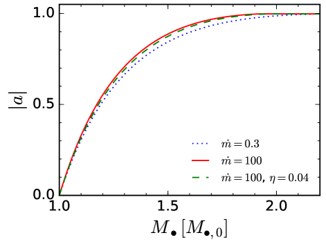
Figure 1.— MBH spin evolution as a function of mass (in unit of the initial mass $M_{{\bullet},0}$) due to coherent-accretion. The blue dotted (red solid) line represents the case of the thin (thick) disc accretion with a constant rate $\dot{m}=0.3\ (100)$ and radiative efficiency $\eta$ derived from $f_{\rm Edd}-\ln\dot{m}$ relation; the green dashed line represents the thick disc accretion with a constant rate of $\dot{m}=100$ and $\eta=0.04$ (for this efficiency, see Jiang et al., 2014).

The spin evolution for an MBH accreting via $\dot{m}=100$ (0.3) is shown as the red solid (blue dotted) line in Figure 1, where the MBH becomes maximally spinning when its mass roughly doubles. Note that our result for $\dot{m}=100$ is only slightly different from that given by Sądowski et al. (2011), in which a detailed slim disc accretion model is adopted to solve the spin evolution equation, with the consideration of photon capture effect. They found that the spin evolution depends on both the viscosity $\alpha$ and the accretion rate $\dot{m}$, and the maximum spin value $a_{\rm max}$ is slightly different from the canonical value $0.998$. For example, with $\alpha=0.1$ and $\dot{m}=1$, the MBH reaches a maximum spin value of $0.9924$ when its mass becomes $\sim 2.4$ times larger. We do not repeat the complicated calculations by Sądowski et al. (2011) for thick disc accretion, as the slight difference in the maximum spin value and the time it reaches the value does not affect our final results much.

Numerical solution of the relativistic slim disc equations (Sądowski, 2009) found that $f_{\rm Edd}$ is also dependent on the MBH spin. Madau et al. (2014) fit the $f_{\rm Edd}-\dot{m}$ relation by adding additional dependence on spin according to the simulation results of Sądowski (2009). We have checked that adopting this spin-dependent relation makes little difference to the spin evolution.

Jiang et al. (2014) claim that super-Eddington accretion could be radiatively more efficient than the $f_{\rm Edd}-\ln\dot{m}$ relation gives. Using magneto-hydrodynamic simulations, they found $\eta\sim 0.04$ for super-Eddington accretion by considering the buoyancy effect. We further check the spin evolution in this case by setting constant efficiency $\eta=0.04$, accretion rate $\dot{m}=100$, and the Eddington ratio $f_{\rm Edd}=16\eta\dot{m}$ (the green dashed line in Fig. 1). It appears that the resulting spin evolution shows little difference comparing to the case of either thin disc accretion with a rate of $\dot{m}=0.3$ (blue dotted line in Fig. 1) or thick disc accretion with $\dot{m}=100$ (red solid line in Fig. 1), both with $\eta$ inferred from the $f_{\rm Edd}-\ln\dot{m}$ relation.

For the coherent-accretion phase, we conclude that different choices of the accretion rate result in only slight difference in the spin evolution as a function of mass (see Fig. 1).

(iii) Chaotic thin disc accretion. We consider multi-episode accretion of gas clouds, and in each episode the clouds infall with random orientations. The accretion rate is assumed to be moderate, i.e., $f_{\rm Edd}=0.3$, and in this case the disc is described by the standard thin disc model (but not necessarily on the MBH’s equatorial plane). Choosing a different $f_{\rm Edd}$ mainly affects the accretion time, and makes little difference to the spin-mass evolutionary curves. The disc orientation is given by the polar angle $\theta$ and azimuthal angle $\phi$ relative to $Oxyz$ (the observer’s rest frame centered on the MBH with $z$ as the direction from the MBH to the distant observer). For each chaotic episode, $\phi$ and $\theta$ are randomly selected from a flat probability distribution over $0$ to $2\pi$ and a probability distribution proportional to $\sin\theta$, respectively, in order to achieve random orientations of the chaotic discs. Different from the coherent thin disc case, the discs considered here are much smaller, and the temporal evolution of the disc involving the LT effect has to be considered. For this part, the procedures to calculate the spin evolution are similar to that provided by Dotti et al. (2013, their model with $F=0.5$), and the only difference is the disc mass in each episode.

The amount of gas that is available for accretion is probably not the same in different accretion episodes. We assume that in each episode, the mass of the gas cloud infalling and to be accreted depends on the MBH mass and is described by

$$M_{\rm cl}=bM_{\bullet}\left(\frac{M_{\bullet}}{10^{8}M_{\odot}}\right)^{\gamma},$$ (4)

where $b$ and $\gamma$ are constant parameters, $M_{\bullet}$ is the MBH mass at the beginning of each episode. If $\gamma=0$, then $M_{\rm cl}$ scales linearly with $M_{\bullet}$; if $\gamma=-1$, then $M_{\rm cl}$ is a constant and is irrelevant to the MBH mass but determined by the environment. In this section, we aim at illustrating how the MBH spin evolves for different settings of $M_{\rm cl}$, and only consider the case with $\gamma=0$ for simplification. In Section 3, we will consider more general cases with $\gamma\neq 0$.

The whole cloud is assumed to form an accretion disk with negligible mass loss, i.e., $M_{\rm disc}=M_{\rm cl}$. The disc size ($R_{\rm disc}$) is estimated via Equation (C3) by applying the surface density profile of standard thin disc, and is then compared with the warp radius ($R_{\rm warp}$; Eq. C7) of the disc which approximately marks the distance of maximally warped region to the central MBH. If $R_{\rm disc}>R_{\rm warp}$, then Equations (1) and (2) are solved by applying the adiabatic approximation (Perego et al., 2009), i.e., the disc transits through a sequence of steady warped states over a short time interval $\delta t\ll t_{\rm al}$, where $t_{\rm al}$ is the alignment timescale. The analytic solution of how the disc is deformed at different radii has been found by Martine et al. (2007), and the analytic expression of the torque term in Equation (2) with respect to the MBH coordinate ($Ox^{\prime}y^{\prime}z^{\prime}$; $z^{\prime}$ is always parallel to ${\bf J}_{\bullet}$) is directly provided by Perego et al. (2009, see their Appendix for power-law viscosity). The variation of ${\bf J}_{\bullet}$ within each $\delta t$ with respect to $Ox^{\prime}y^{\prime}z^{\prime}$ is then rotated back to the observer’s rest frame (see Perego et al., 2009; Dotti et al., 2013, for details).

If the inequality $R_{\rm warp}>R_{\rm disc}$ holds, then the angular momentum of the MBH is assumed to be instantaneously aligned with the total angular momentum ${\bf J}_{\rm tot}(={\bf J}_{\rm disc}+{\bf J}_{\bullet})$. The re-orientation of the MBH spin is rather small since ${\bf J}_{\bullet}$ dominates over ${\bf J}_{\rm disc}$. The disc goes through a fast and significant re-orientation, and whether the disc angular momentum is aligned or anti-aligned with the MBH spin is determined by the disc-to-MBH angular momentum ratio and the angle $\beta$ between ${{\bf J}_{\rm disc}}$ and ${\bf J}_{\bullet}$. If $\cos\beta>-J_{\rm disc}/2J_{\bullet}$, then they are aligned; otherwise, anti-aligned (King et al., 2005). In this case, we only need to solve Equation (3) that governs the spin module evolution for each single chaotic accretion episode. This is similar to that for the coherent accretion case, except that anti-alignment is possible here and the direction of the MBH spin is re-oriented to the total angular momentum direction for each chaotic accretion episode.

It is proposed that the accretion disc cannot be too massive, as it may be unstable against its own gravity and can be fragmented into gas clumps at the outer region when the disc is too massive (e.g., Kolykhalov & Sunyaev, 1980; Goodman & Tan, 2004; King et al., 2008). The criterion for disc instability is given by Toomre-$Q=1$, which yields a maximum disc size $R_{{\rm disc},{\rm sg}}$, and this corresponds to a maximum disc mass $M_{\rm sg}$ (see Appendix C for details). Although there could be such an upper limit for the disc mass, the infalling of gas clumps onto the outer disc and other mechanisms may also heat the disc significantly and thus prevent it from fragmentation. Therefore, we consider two cases: one case is that the disc is not affected by the possible instabilities due to its self-gravity (not limited by $M_{\rm sg}$) for which $M_{\rm disc}=M_{\rm cl}$, and the other is that the disc mass is indeed regulated by self-gravity, i.e., $M_{\rm disc}=\min(M_{\rm cl},M_{\rm sg})$. If not otherwise stated, we will mainly focus on the former case, while the latter case will be investigated in details in Section 3.

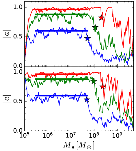
Figure 2.— Examples for spin modulus evolution of MBHs undergoing chaotic accretion. These MBHs are assumed to have initial masses of $10^{5}M_{\odot}$, initial spins of either $0$ (top panel) or $0.998$ (bottom panel), and grow up via chaotic accretion with many episodes with $M_{\rm disc}=bM_{\bullet}$ in each episode, where $b=0.003$ (blue line), $0.01$ (green line), or $0.03$ (red line). Star symbols mark the critical MBH mass given by $R_{\rm disc}=R_{\rm warp}$. For each curve shown here, the horizontal line with the corresponding color indicates that the spin modulus oscillates around an equilibrium value when the MBH mass is smaller than the critical MBH mass.

Figure 2 shows examples of spin evolution for several MBHs accreting chaotically with $M_{\rm disc}=bM_{\bullet}$ in each episode. Whatever the initial spin is ($0$ or $0.998$), the MBH spin quickly reaches a quasi-equilibrium state when the MBH mass roughly doubles and then fluctuates around the equilibrium value until $M_{\bullet}\sim 10^{8}M_{\odot}$. For initially non-rotating MBHs, the sharp increase at the beginning is due to the short alignment timescale. The MBH spin is quickly re-aligned to ${\bf J}_{\rm tot}$, which is approximately parallel with ${\bf J}_{\rm disc}$ because ${\bf J}_{\rm disc}$ dominates over ${\bf J}_{\bullet}$ when the MBH mass is low, leading to an increase in spin with time. For initially maximally spinning MBHs, the (sharp) decrease of the spin can be similarly explained. How large the equilibrium value $a_{\rm eq}$ could reach depends on the disc mass in each episode, i.e., the $b$ value. The dependence of $a_{\rm eq}$ on $b$ is shown in Figure 3, and each point with error bar (one standard deviation) is obtained from $200$ realizations of Monte Carlo simulations. But in general choosing a different set of $\alpha$ and $f_{\nu_{2}}$ only slightly affects those constraints obtained on MBH growth obtained in Section 3. How spin modulus evolves is determined by the competition of prograde and retrograde accretion. For ideal chaotic case, the number of prograde and retrograde episodes are the same, and thus the MBH spin appears to decrease with time since retrograde accretion is more efficient in angular momentum injection. However, the spin also precesses and tends to align with the disc angular momentum. Hence, what matters is whether the spin could align efficiently within a single accretion episode. If yes, then the accretion will quickly transit to prograde even if it starts with retrograde, and then the spin increases.

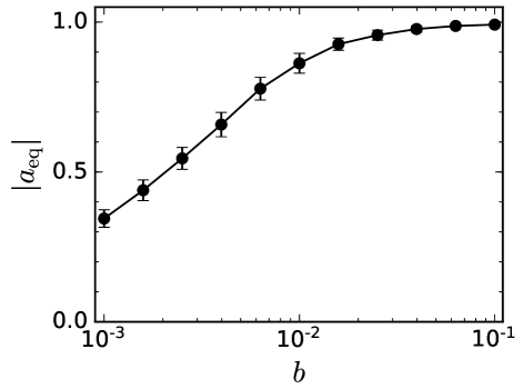
Figure 3.— Dependence of the equilibrium spin value on the disc mass (characterized by $b$) for MBHs undergoing chaotic accretion (see the horizontal lines shown in Fig. 2). The black circles and their associated error bars show the mean values and their standard deviations resulting from 200 realizations of Monte Carlo simulations.

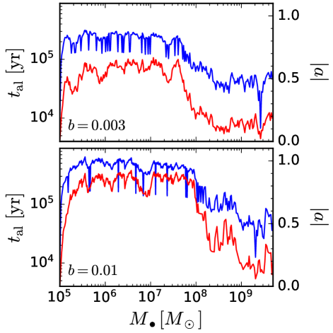
Figure 4.— Examples for the evolution of the alignment timescale $t_{\rm al}$ (left y-axis; blue lines) and the MBH spin modulus (right y-axis; red lines) with the mass growth of MBHs undergoing chaotic accretion with $M_{\rm disc}=0.003M_{\bullet}$ (top panel) and $0.01M_{\bullet}$ (bottom panel) in each episode. The red lines in the top (bottom) panel are the same as the blue (green) lines in the top panel of Fig. 2.

Figure 4 shows coupled evolution of the alignment timescale and the MBH spin for $b=0.003$ (top panel) and 0.01 (bottom panel), where the alignment timescale is evaluated by $t_{\rm al}\approx 10^{5}\alpha^{58/35}_{0.1}f^{-5/7}_{\nu_{2}}M^{-2/35}_{{\bullet},6}\left(\frac{f_{\rm Edd}}{\eta_{0.1}}\right)^{-32/35}a^{5/7}\rm{yr}$ (Perego et al., 2009). As seen from this figure (see also the blue and green curve in Fig. 2), the spin roughly maintains at an equilibrium value and oscillates around it when the MBH mass is around a few times $10^{5}M_{\odot}$ to a few times $10^{7}M_{\odot}$. This quasi-equilibrium state can be explained as follows. An increase in spin leads to an increase in $t_{\rm al}$ ($\propto a^{5/7}$); a less efficient alignment leads to a decrease of spin; hence the spin oscillates. With further increase of the MBH mass, the disc size may reach a critical value of $R_{\rm disc}=R_{\rm warp}$, and after that the MBH spin leaves the quasi-equilibrium state. When $R_{\rm disc}<R_{\rm warp}$, the MBH and disc angular momenta are assumed to be instantaneously aligned or anti-aligned with each other, and thus the spin tends to decline on average with increasing MBH mass after $R_{\rm disc}=R_{\rm warp}$ (the transition is shown as the star symbols in Fig. 2). How fast the spin decreases is determined by the relative fraction of prograde and retrograde episodes, which mainly depends on $J_{\rm disc}/J_{\bullet}$, and thus $b$ [see Eq. (C6)].

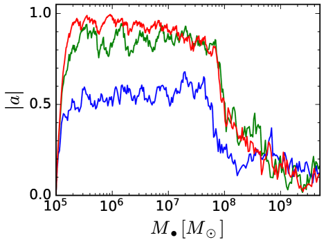
Figure 5.— Example spin modulus evolutionary curves for MBHs undergoing chaotic accretion by considering the self-gravity of the disc in each accretion episode. The MBH initial masses and spins are fixed to be $10^{5}M_{\odot}$ and 0, respectively, and the disc mass in each accretion episode is assumed to be $M_{\rm disc}=\min(bM_{\bullet},M_{\rm sg})$, where $b=0.003$ (blue), $0.01$ (green), or $0.03$ (red). The slight decline of the equilibrium spin value with increasing $M_{\bullet}$ (from $\sim 3\times 10^{5}$ to $6\times 10^{7}M_{\odot}$) shown by the red line is due to the decrease of the mean disc-to-MBH mass ratio .

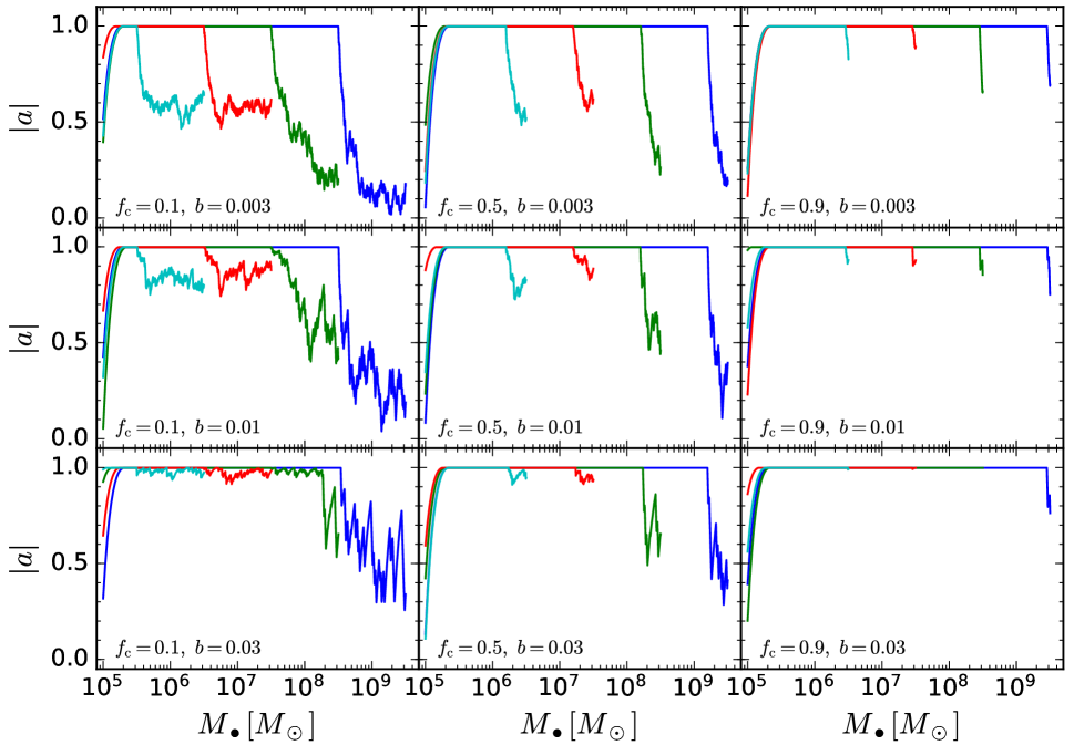
Figure 6.— Examples spin modulus evolutionary curves of MBHs undergoing two-phase accretion with $\gamma=0$, $f_{\rm c}=0.1$ (left), $0.5$ (middle) or $0.9$ (right), $b=0.003$ (top), $0.01$ (middle), or $0.03$ (bottom). The final masses of the MBHs are $M_{\bullet,\rm f}=3\times 10^{6}M_{\odot}$ (cyan), $3\times 10^{7}M_{\odot}$ (red), $3\times 10^{8}M_{\odot}$ (green), or $3\times 10^{9}M_{\odot}$ (blue). The initial masses here are fixed at $10^{5}M_{\odot}$, and the initial spins are randomly generated between 0 and 1.

Figure 5 shows the spin evolution of MBHs undergoing chaotic accretion by considering the self-gravity of the accretion disc. For the case with small $b$, i.e., $b=0.003$ (blue line), it is similar to that shown in Figure 2 without consideration of disc self-gravity, because $M_{\rm cl}<M_{\rm sg}$ is valid almost in the whole accretion history of the MBH. For $b=0.01$, however, self-gravity plays an important role when $M_{\bullet}\gtrsim 2\times 10^{7}M_{\odot}$ ($M_{\rm cl}\gtrsim M_{\rm sg}$). Therefore, the MBH spin magnitude decreases faster and reaches a lower value when the MBH mass is high (larger than a few times $10^{8}M_{\odot}$), compared with that shown in Figure 2. For $b=0.03$, self-gravity is always important in the accretion history of the MBH. In this case, the equilibrium spin value slightly decreases with increasing MBH mass because of the decrease of $b\ (=M_{\rm sg}/M_{\bullet})$ with increasing $M_{\bullet}$, and the MBH spin decreases as fast as that with $b=0.01$ when $R_{\rm disc}>R_{\rm warp}$, and reaches similarly low values at the high-mass end (red curve in Fig. 5).

3. Observational constraints on MBH accretion history via spin and mass distribution

Currently there are more than two dozen AGNs that have relatively robust spin measurements via the X-ray reflection spectroscopy (see Table 1) as mentioned in the Introduction. About two thirds of these AGNs have spins $>0.8$, and the rest have intermediate spins $\sim 0.4-0.8$. In this section, we aim at using the distribution on the mass versus spin plane of this sample to constrain the accretion history of MBHs.

We assume that all MBHs experience an initial coherent-accretion phase and a later chaotic-accretion phase. For an MBH with initial mass $M_{\bullet,0}$ and final mass $M_{\bullet,\rm f}$, it grows up through coherent accretion before its mass reaches a factor $f_{\rm c}$ of $M_{\bullet,\rm f}$, and after that, it enters to the second phase and grows via chaotic accretion as argued in Section 2. The disc mass in each chaotic accretion episode is assumed to be described by Equation (4). For such a two-phase accretion model, parameters that are interesting in this paper are mostly $f_{\rm c}$ and $b$ if $\gamma$ is fixed.

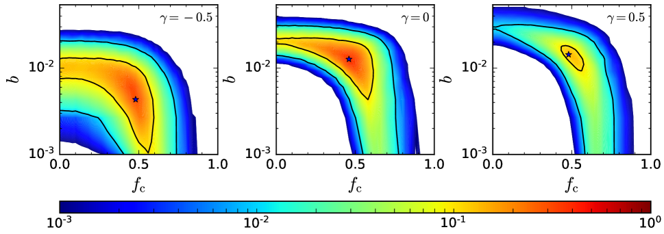
Figure 7.— Constraints on the parameters $b$ and $f_{\rm c}$ in the two-phase accretion model from the available spin measurements of AGNs listed in Table 1. Colors represent the $P$-value obtained from the 2D-Kolmogorov-Smirnov (2D-KS) test as indicated by the color bar at the bottom of this figure. Panels from left to right are for the cases with $\gamma=-0.5$, $0$, and $0.5$, respectively. Star symbol in each panel marks the location with the largest 2D-KS $P_{\rm KS}$ value, which is $(f_{\rm c},\ b)=(0.48,\ 0.004)$, $(0.46,\ 0.012)$, and $(0.48,\ 0.014)$, respectively from the left to right panel. The black lines mark $P_{\rm KS}=0.1$ and 0.01. The white region that is not filled with colors has $P_{\rm KS}<0.001$ and therefore can be excluded. Note here we simply adopt the lower limit of the color bar as $0.001$ in order to make the color gradient more clear for the rest parts.

Figure 6 shows the spin evolutionary tracks of a few MBHs by assuming such two-phase accretion models with $\gamma=0$ and different sets of the other two parameters ($f_{\rm c}$, $b$). If $f_{c}$ is small and thus the chaotic-accretion phase dominates the MBH growth (left panels of Fig. 6), then the initial coherent-accretion phase makes the spin increase quickly to the canonical value $0.998$, and it maintains until the chaotic accretion phase makes it decrease somewhat. Afterwards it oscillates around an equilibrium value depending on the value of $b$. If $M_{\bullet,\rm f}$ is larger than several times $10^{8}M_{\odot}$, the MBH spin further decreases to small values (close to $0$) in the late chaotic accretion phase. If $f_{\rm c}$ is large (e.g., $0.9$; right panels of Fig. 6), the chaotic-accretion phase is not significant for the MBH growth and thus the de-spin may only occur in a short period of the later life of a QSO since $f_{\rm c}$ determines fraction of its lifetime with spin close to $1$ and the time left to the chaotic-accretion phase (cf., right panels of Fig. 6). Note that the value of $b$ (or $M_{\rm disc}$ in each episode) determines how efficiently the MBH could be spun down in a single chaotic accretion episode.

In order to obtain constraints on the MBH growth history from the observationally measured MBH spin and mass distribution, we first generate a large number of mock MBHs for different settings of the model parameters $(b,\ f_{\rm c},\ \gamma)$. We assume that the final masses of those MBHs follow the mass distribution of local AGNs (Schulze & Wisotzki, 2010) since almost all MBHs with spin measurements are at redshift $z<0.3$.

We randomly generate $4000$ MBHs over the logarithmic final mass ranging from $10^{6}$ to $10^{10}M_{\odot}$. Then we adopt the accretion model described in Section 2 to calculate the spin evolution curves for these $4000$ MBHs with each given set of parameters ($f_{\rm c}$, $b$, $\gamma$), and take these spin evolution curves as templates. Using the mass distribution function as the weight, we randomly select mock AGNs and thus the AGN properties from those templates, including the MBH mass and spin at the ‘observation’ time.

For the spin curve calculation, we set the initial masses of those MBHs randomly distributed from $10^{4}$ to $10^{5}M_{\odot}$ in the logarithmic space and the initial spins are randomly distributed from $0$ to $1$. In the coherent-accretion phase, we set the accretion rate as $\dot{m}=0.3$. A different choice of the accretion rate at the coherent-accretion stage makes little difference to the spin evolution as suggested by Figure 1 and described in Section 2. We will further discuss in Section 4, however, a different choice of $\dot{m}$ does cause some difference on the frequency of those MBHs accreting via thin disc and thus emitting Fe K$\alpha$ line in the inner disc region at the early stage of MBH growth. In the chaotic thin disc accretion phase, we assume that the Eddington ratio $f_{\rm Edd}$ in each episode is a constant, and $\log f_{\rm Edd}$ is randomly drawn from a Gaussian distribution with mean $-0.8$ and standard deviation $0.5$. We have checked and found that it makes little difference to our results if $f_{\rm Edd}$ is drawn from the distribution of local active MBHs (Schulze & Wisotzki, 2010), but the time needed to select mock samples with appropriate luminosity is much longer.

With these settings, we obtain the spin evolution curves for those MBHs by solving Eqs. (1) and (2) or (3). For each MBH, we record the mass, spin, and bolometric luminosity ($f_{\rm Edd}L_{\rm Edd}$) every $4.5\times 10^{4}$ yr ($\sim 10^{-4}t_{\rm Edd}$). For the $i$-th observed AGN with mass $M_{i,{\rm obs}}$, spin $a_{i,{\rm obs}}$, and luminosity $L_{i,{\rm obs}}$ listed in Table 1, we randomly select an evolution curve and a random moment $t_{i}$ in the curve for the period via thin disc accretion, and then obtain the mass $M_{i,\rm mock}$ and bolometric luminosity $L_{i,\rm mock}$ of a mock AGN at that moment by interpolation. The masses of active MBHs in Table 1 are mostly determined through the empirical virial mass estimators, which may deviate from the true masses with a scatter of $0.3-0.4$ dex (e.g., Shen et al., 2008, 2011, see also Vestergaard & Peterson 2006). The bolometric luminosity is usually derived from a combination of the luminosity at a specific band with the corresponding bolometric correction. The bolometric corrections for a specific optical band usually have a scatter of 0.1-0.2 dex (e.g., Hopkins et al., 2007). In addition, there are other uncertainties, such as those induced by absorption and host contamination, which are difficult to accurately consider. We therefore set an empirical uncertainty of 0.3 dex, and select a mock AGN as a correspondence to the $i$th object in Table 1 if $\left|\log(M_{i,\rm mock}/M_{i,{\rm obs}})\right|<0.3$, and $\left|\log(L_{i,\rm mock}/L_{i,{\rm obs}})\right|<0.3$. The spin $a_{i,\rm mock}$ at that moment is obtained by interpolation. If these inequalities are not satisfied, then we select another curve and repeat the above processes. For each observed source, we generate $1,000$ mock objects. Choosing a larger number does not affect our final results. After going through all the 27 observed sources, we obtain $27\times 1000=27,000$ mock objects. The we obtain the spin-mass distribution output from each model according to these mock objects.

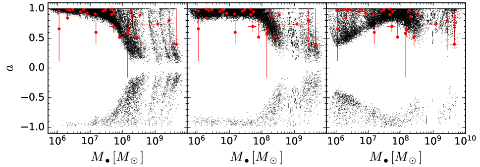
Figure 8.— Spins of the AGN mock samples (black dots) generated from the two-phase accretion model and spins of the observed AGNs listed in Table 1 (red filled circles with error bars). Left, middle, and right panels represent $(f_{\rm c},\ b,\ \gamma)=(0.48,\ 0.004,\ -0.5)$, $(0.46,\ 0.012,\ 0)$, and $(0.48,\ 0.014,\ 0.5)$, respectively, corresponding to the cases marked by the star symbols in Fig. 7.

For those objects with spin measurements listed in Table 1, we assume a probability distribution function (PDF) for each source by considering the spin measurement errors listed there (see similar assumptions made in Sesana et al. 2014). For objects given with symmetric spin errors, a Gaussian PDF is assumed; for those given with asymmetric errors, we assume the PDF is composed of two half-Gaussians; for those given with lower limits, the PDF is assumed to have 90% probability randomly distributed between $0.998$ and the lower limit (90% CL), and 10% probability to lie between $-0.998$ and the lower limit. We randomly assign a spin to each of the $27$ object according to this assumed probability distribution for each object, and obtain a spin-mass distribution for the observational sample. We compare this ‘observational’ spin-mass distribution with the model spin-mass distribution via the two-dimensional Kolmogorov-Smirnov (2D-KS) test (Press et al., 2007), and obtain the $P_{\rm KS}$ value. Although the 2D-KS test is not as rigorous as its one-dimensional counterpart, it does return a p-value $P_{\rm KS}$ which demonstrates the approximate probability that the two samples are drawn from the same distribution. We repeat the above process for $1000$ times and obtain $1000$ $P_{\rm KS}$ values for each model. We take the median of those $P_{\rm KS}$ as the true $P_{\rm KS}$ value for a given model. In such a way, we can investigate whether a model with one set of $(f_{\rm c},b,\gamma)$ matches the observational spin-mass distribution better than another one by comparing the $P_{\rm KS}$ values.

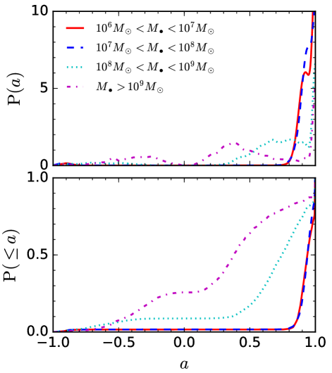
Figure 9.— Differential (top panel) and cumulative (bottom panel) spin distribution of the mock AGN sample generated from the reference model (black dots in the middle panel of Figure 8) in different mass range, i.e., $10^{6}M_{\odot}<M_{\bullet}<10^{7}M_{\odot}$ (red solid), $10^{7}M_{\odot}<M_{\bullet}<10^{8}M_{\odot}$ (blue dashed), $10^{8}M_{\odot}<M_{\bullet}<10^{9}M_{\odot}$ (cyan dotted), and $M_{\bullet}>10^{9}M_{\odot}$ (magenta dot-dashed).

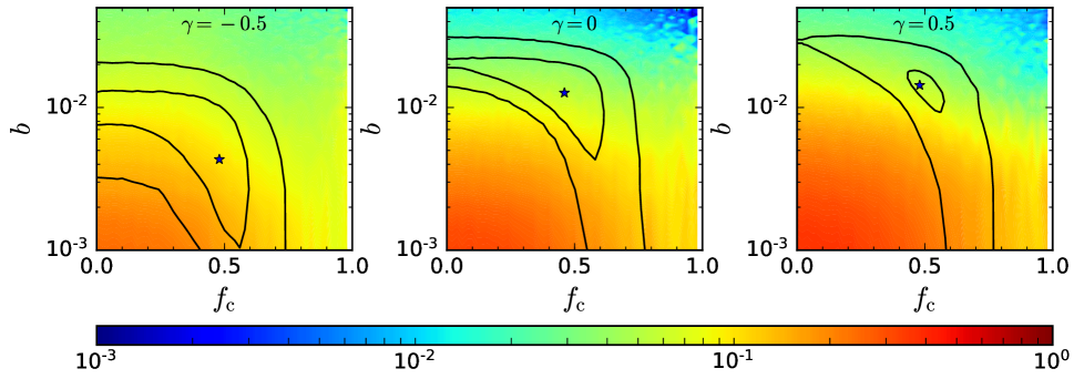
Figure 10.— Fraction of negative spins (i.e., retrograde accretion) in the parameter space of $(f_{\rm c},\ b)$ assuming $\gamma=-0.5$ (left panel), $0$ (middle panel), and $0.5$ (right panel). The star symbols mark the location of the model parameters that leads to the largest $P_{\rm KS}$ value, and the black lines show $P_{\rm KS}=0.1$ and $0.01$, as shown in Fig. 7. The small white regions are for the fraction of negative spins $<0.001$.

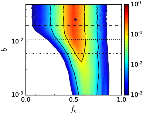
Figure 11.— Legends similar to that for the middle panel of Fig. 7, but considering the self-gravity of the thin disc at the chaotic-accretion phase. Similarly, the star symbol marks the location of the highest $P_{\rm KS}$ value $(f_{\rm c},b)=(0.52,0.026)$. The black solid lines show $P_{\rm KS}=0.1$ and $0.01$, respectively. The dashed/dotted/dot-dashed line marks the upper limit of $b$ for an MBH with mass $M_{\bullet}>10^{6}M_{\odot}$/$10^{7}M_{\odot}$/ $10^{8}M_{\odot}$, above which the disc is fragmented due to its self-gravity. As seen from this Figure, self-gravity of the disc may play a dominant role when $b$ is substantially larger than one percent for $M_{\bullet}>10^{6}-10^{7}M_{\odot}$.

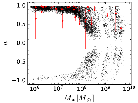
Figure 12.— Legend similar to Fig. 8 but with consideration of the self-gravity of discs at the chaotic-accretion phase.

We first consider the general case that the disc mass in each episode of chaotic accretion $\propto M^{1+\gamma}_{\bullet}$ [Eq. (4)]. Figure 7 shows the distribution of $P_{\rm KS}$ on the plane of $b$ versus $f_{\rm c}$. For simplification, we set three different values for $\gamma$, i.e., $-0.5$, $0$, and $0.5$ (from left to right panels), to check whether the model with a positive or negative $\gamma$ can match the observed spin distribution better, comparing to the model with $\gamma=0$. According to those models with different $\gamma$ values as shown in Figure 7, it can be excluded with at least $99.9\%$ confidence level that the spin distributions of the mock samples produced from those models with $f_{\rm c}>0.9$ and that of the observed sample come from the same distribution, which means that chaotic accretion is required and contributes at least $10\%$ to the MBH final mass. Figure 7 also shows a trend that a smaller $b$ allows for a larger $f_{\rm c}$. This is because a smaller $b$ means a smaller disc and a more efficient decrease in spin in the chaotic-accretion phase and a larger $f_{\rm c}$ implies less time left for chaotic accretion. To reproduce the observed fraction of intermediate spins (e.g., $\sim 0.4-0.8$), $b>0.05$ can also be excluded at $99.9\%$ confidence level as it results in too many MBHs with spins close to $1$. Note that $f_{\rm c}\lesssim 0.01$ cannot be excluded (especially for $\gamma=0$; middle panel), because chaotic accretion alone can also lead to the observed intermediate-to-high spin distribution if the the disc mass (represented by $b$) is appropriate, i.e., neither too large nor too small. As seen from Figure 7 (and also Fig. 8), it appears that the model with $\gamma=0$ matches the observations ($P_{\rm KS}\sim 0.4$) better than that with $\gamma=0.5$ or $-0.5$. There also seems to be a trend that a model with smaller $\gamma$ requires a smaller $b$ to generate mock samples matching the observation. The reason is that a smaller $\gamma$ should be coupled with a smaller $b$ (and vice versa) in order to maintain an appropriate disc mass [$\propto bM_{\bullet}\left(M_{{\bullet}}/10^{8}M_{\odot}\right)^{\gamma}$] that can lead to the scatter of spins in the mass range from a few times $10^{7}M_{\odot}$ to a few times $10^{8}M_{\odot}$.

Figure 8 shows the corresponding spin-mass distributions of the mock samples given by those models with the largest $P_{\rm KS}$ value, i.e., $(f_{\rm c},\ b,\ \gamma)=(0.48,\ 0.004,\ -0.5)$ (left panel), $(0.46,\ 0.012,\ 0)$ (middle panel; hereafter the reference model), and $(0.48,\ 0.014,\ 0.5)$ (right panel), respectively. As seen from this figure, the distributions of the mock AGNs obtained from the model with the highest $P_{\rm KS}$ value but different $\gamma$ show different patterns, especially at the low mass end. For the model with $\gamma=0.5$, the mock AGNs with $M_{\bullet}\lesssim 10^{7}M_{\odot}$ have intermediate to high spins $(\sim 0.5-1)$, while they mostly have high spin $(\gtrsim 0.8$) for the model with $\gamma=-0.5$.

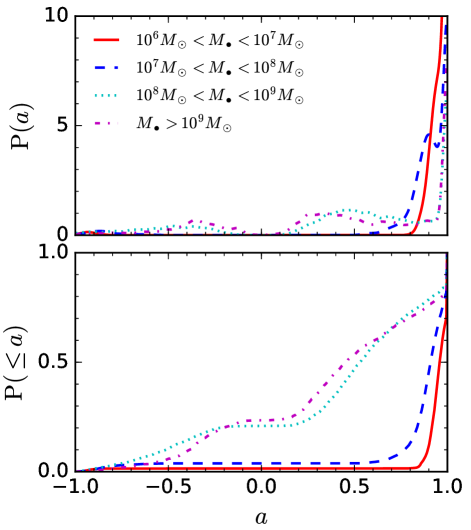
Figure 13.— Legend similar to Fig. 9 but considering the self-gravity of discs at the chaotic-accretion phase.

Figure 9 shows the differential and cumulative spin distributions of those mock objects in different mass bins, in order to illustrate how the spin distribution depends on the MBH mass. As seen from this figure, higher mass MBHs ($>10^{8}M_{\odot}$) have relatively low spins, which is a natural result of the two-phase accretion model as chaotic-accretion phase normally leads to a fast spin-down of heavy MBHs at their later growth stage (see Figs. 2, 5, and 6). It is also prominent that a fraction of MBHs have negative spins. The reason is that $J_{\rm disc}/J_{\bullet}$ decreases with increasing MBH mass for a given $b$ at the chaotic accretion phase [Eq. (C6)], and the criterion for anti-alignment $\cos\beta<-J_{\rm disc}/2J_{\bullet}$ (King et al., 2005) can be satisfied in some cases.

Figure 10 shows the fraction of mock AGNs that have negative spins on the plane of $f_{\rm c}$ versus $b$, obtained from those models with $\gamma=-0.5$ (left panel), $0$ (middle panel), and $0.5$ (right panel), respectively. A model with smaller $b$ results in a larger fraction of AGNs with negative spins, because $J_{\rm disc}/J_{\bullet}$ is smaller, and the criterion for anti-alignment (see King et al., 2005) can be more frequently satisfied. A larger fraction of negative spins can also result from models with smaller $f_{\rm c}$ but the same $b$, as the duration of the chaotic-accretion phase is longer and thus there are more chances to have anti-aligned accretion disc. The model with the largest $P_{\rm KS}$ value, i.e., $(f_{\rm c},\ b)=(0.46,\ 0.012)$ results in $\sim 5.5\%$ of the mock AGNs that have negative spins, i.e., roughly $1.5$ in $27$ objects. According to Figure 9, however, one may note that the fraction of counter-rotating MBHs depends on the MBH mass, i.e., the higher the MBH mass, the higher the fraction (see Discussion part).

If we consider self-gravitated discs in the chaotic-accretion phase, i.e., $M_{\rm disc}=\min(bM_{\bullet},M_{\rm sg})$ if $\gamma=0$, then we can also obtain the distribution of $P_{\rm KS}$ value on the plane of $f_{\rm c}$ versus $b$ according to the same processes described above (as shown in Figure 11). Here $M_{\rm sg}$ is the maximum mass of an accretion disc by considering self-gravity and disc fragmentation and it is given in Appendix (Eq. C10). Similar to the previous results, $f_{\rm c}$ is also constrained to be less than $\sim 0.85$ at $\gtrsim 99.9\%$ confidence level, and the location of the model with the largest $P_{\rm KS}$ value is $(f_{\rm c},\ b)=(0.52,\ 0.026)$, roughly consistent with the previous results. It seems that a large $b$ is now allowed, apparently different from those models without consideration of disc self-gravity. The reason for this difference is straightforward, i.e., the disc mass is determined by $M_{\rm sg}$ for those models with large $b$, in which $b$ does not play a role because $M_{\rm sg}<bM_{\bullet}$. By setting $M_{\rm sg}=bM_{\bullet}$, we may obtain a critical MBH mass below which $M_{\rm disc}=bM_{\bullet}$ and above which $M_{\rm disc}=M_{\rm sg}$. This critical mass is determined by $b$. If we set the critical mass as $10^{6}M_{\odot}$, it means that the masses of discs around all MBHs with $M_{\bullet}>10^{6}M_{\odot}$ are limited to $M_{\rm sg}$, and the corresponding $b$ value must be $\leq 0.02$ (as indicated by the dashed line in Fig. 11). For a critical MBH mass of $10^{7}M_{\odot}$ or $10^{8}M_{\odot}$, it gives an upper limit of $b=0.011$ (dotted line) or 0.006 (dot-dashed line in Fig. 11).

Figure 12 shows the mock sample obtained from the two-phase accretion model with the largest $P_{\rm KS}$ value by considering self-gravity of the disc in the chaotic-accretion phase, i.e., $(f_{\rm c},\ b,\ \gamma)=(0.52,\ 0.026,\ 0)$, as a comparison to the spin-mass distribution shown in the middle panel of Figure 8. Figure 13 shows the spin distribution of the mock AGNs in Figure 12 for different mass ranges. By comparing these two figures with Figures 8 and 9, we find that qualitatively the results obtained with and without consideration of disc self-gravity do not differ much.

4. Discussion

4.1. Different choices of the accretion rate in the coherent- and chaotic-accretion phases

In our calculations presented in the previous section, the accretion rate in the coherent-accretion phase is set to be a constant, i.e., $\dot{m}=0.3$. However, the accretion in the coherent phase can also be super-Eddington. Therefore, we further check the case with $\dot{m}=100$ and do similar calculations. Figure 14 shows the distribution of $P_{\rm KS}$ obtained from models with $\gamma=0$ and $\dot{m}=100$ in the coherent-accretion phase. We find that those models with large $f_{\rm c}$ (e.g., $0.9<f_{\rm c}<0.95$) here can still be compatible with the observations, and the model with the largest $P_{\rm KS}$ value is $(f_{\rm c},\ b)=(0.80,\ 0.009)$. For comparison, models with $f_{\rm c}>0.9$ are ruled out with a high confidence $99.9\%$ if $\dot{m}=0.3$ (middle panel of Figure 7). The reason is that the time for the coherent super-Eddington accretion phase is short, and even if $f_{\rm c}=0.9$, for example, there is still 10% of chaotic thin disc accretion for the MBH growth, from which mock objects can be selected to match the observational spin distribution. In contrast, if $\dot{m}=0.3$ and $f_{\rm c}=0.9$, then the probability is high to select mock objects in the coherent phase, when most MBHs are maximally spinning, and thus this model overproduces MBHs with spins close to $1$, especially when MBHs are large ($>10^{8}M_{\odot}$).

In addition, the accretion rate in the coherent stage may change with time. Levinson & Nakar (2018) have shown that the accretion rate of MBHs at early epochs can not exceed

$$\dot{M}_{\rm acc}\sim 20\left(\frac{\sigma}{350\ {\rm km\,s^{-1}}}\right)^{4}M_{\odot}\ \rm{yr^{-1}},$$ (5)

where $\sigma$ is the stellar velocity dispersion. Considering the $M_{\bullet}-\sigma$ relation, i.e., $M_{{\bullet},f}$ roughly proportional to $\sigma^{4}$ (see Tremaine et al., 2002), we have

$$\dot{M}_{\rm acc}\sim 1.4\frac{M_{\bullet,f}}{10^{8}M_{\odot}}M_{\odot}{\rm\,yr}^{-1}\sim 0.65\frac{M_{\bullet,f}}{M_{\bullet}}\dot{M}_{\rm Edd}(M_{\bullet}).$$

The accretion rate at the early stage ($M_{\bullet}\ll M_{\bullet,f}$) is significantly higher than the Eddington rate and scales with the MBH final mass. We therefore use the above $\dot{M}_{\rm acc}$ as the accretion rate in the coherent phase to perform similar calculations as in Section 3. Figure 15 shows the distribution of $P_{\rm KS}$ on the plane of $f_{\rm c}$ versus $b$. The location for the largest $P_{\rm KS}$ is $(f_{\rm c},\ b)=(0.58,\ 0.011)$, which is in between that obtained by assuming $\dot{m}=0.3$ (middle panel of Fig. 7) and $\dot{m}=100$ (Fig. 14), and only slightly differs from them. This is a natural result because a constant $\dot{M}_{\rm acc}$ in the coherent phase for an MBH with given $M_{\bullet,\rm f}$ means a decreasing $\dot{m}$ with increasing MBH mass, from super-Eddington (e.g., $\dot{m}=100$ at $M_{\bullet}<10^{6}M_{\odot}$) to sub-Eddington (e.g., $\dot{m}\sim 0.3$ when $M_{\bullet}$ is close to $M_{\bullet,\rm f}$).

In our models, the Eddington ratio is also assumed to be constant within each accretion episode and randomly generated for each episode in the chaotic accretion phase. It may be more realistic to assume a time-varying Eddington ratio (or accretion rate) for each episode, i.e., a power-law decay of $f_{\rm Edd}$ or accretion rate (e.g. Yu et al., 2005; Hopkins & Hernquist, 2006; Aversa et al., 2015). However, choosing a different Eddington ratio makes little difference to the spin-mass evolutionary curve, although the accretion time and the light curve can be quite different. It has an equivalent effect by assuming a constant $f_{\rm Edd}$ in a single chaotic accretion episode but varying $f_{\rm Edd}$ in different episodes if the number of accretion episode is large.

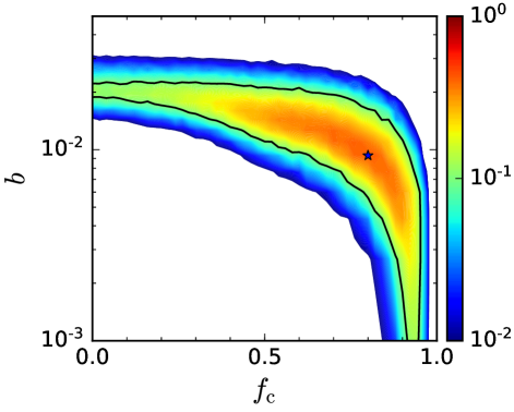
Figure 14.— Constraints on the parameters $b$ and $f_{\rm c}$ in the two-phase accretion model from the available spin measurements of AGNs listed in Table 1. Here the accretion rate at the coherent-accretion phase is set to be super-Eddington with $\dot{m}=100$. The star symbol marks the location with the largest $P_{\rm KS}$ value $(f_{\rm c},\ b)=(0.80,\ 0.009)$. The black contour shows $P_{\rm KS}=0.1$.

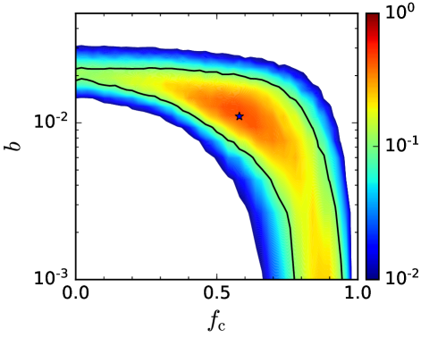
Figure 15.— Legend similar to Fig. 14. However, here the accretion rate in the coherent-accretion phase is set to be the possible upper limit for the accretion rate given by Levinson & Nakar (2018). The star symbol marks the location of the largest $P_{\rm KS}$, i.e., $(f_{\rm c},\ b)=(0.58,\ 0.011)$.

It is apparent that $f_{c}>0.95$ can be excluded at $\sim 99\%$ confidence level although different settings on the accretion rates for the coherent-accretion phase may result in different constraints on model parameters, which means chaotic accretion is necessary. Pure chaotic accretion is still allowed, and in this case $b$ is all constrained to be around 0.01, i.e., $0.007<b<0.03$.

To close this sub-section, we note here that the simple two-phase accretion model adopted in the present paper has some limitations as it ignores the possibility that the accretion history could be much more complicated. For example, the accretion histories may be different for those MBHs in different environments, activated at different redshifts, or with different masses (e.g., Fiacconi et al., 2018). In a much more comprehensive cosmological co-evolution model for MBHs (both masses and spins) and galaxies, one may be able to consider all those complications and obtain detailed constraints on the MBH accretion histories (e.g., see Sesana et al., 2014; Lapi et al., 2006; Shen, 2009). With such a model, one can also simultaneously obtain the QSO luminosity function, the clustering of QSOs, and compare them with observations. However, there are also many more uncertainties because of poor understanding of many physical processes involved in the co-evolution of MBHs and galaxies.

4.2. Mass-dependence of $f_{\rm c}$ and $b$

One of the settings in our previous calculations is that $f_{\rm c}$ and $b$ are both the same for all MBHs. This may not be the fact as $f_{\rm c}$ (and/or $b$) may depend on the MBH (final) mass.

In order to test this possibility, on the one hand, we assume a simple power-law form $f_{\rm c}=f_{0}(M_{{\bullet},\rm f}/10^{8}M_{\odot})^{x}$, and fix $b$ at $0.012$ (the $b$ value of the reference model). By matching the observational spin distribution through the 2D-KS test, we find that the parameters of the model with the largest $P_{\rm KS}$ value are now $(f_{0},\ x)=(0.38,\ 0.06)$. If alternatively adopting $b=0.02$ or $b=0.005$, we obtain $(f_{0},\ x)=(0.10,\ 0.16)$ or $(0.46,\ 0)$. These results imply that there is no necessity to assume an $f_{\rm c}$ dependent on the final MBH mass to match the currently available spin measurements. However, if $f_{\rm c}$ for high-mass MBHs is much smaller than that for low-mass ones (with $b$ fixed at the value of the reference model), the fraction of slowly spinning MBHs at the high mass end would be substantially larger, while if $f_{\rm c}$ for low-mass MBHs is relatively small compared with that for high-mass ones, there will be little change in the resulting spin distribution at the low mass end provided that $b$ is not too small (e.g., $b>10^{-3}$).

On the other hand, if $b$ is, not necessarily monotonically, dependent on the final MBH mass, then the resulting MBH spin distribution may be significantly different from the reference model. Assuming $b\propto M^{\kappa}_{\bullet,f}$ is similar to the setting described by Equation (4), and therefore, its effects on the MBH spin distribution can be seen from Figure 8. However, if $b$ is less than $0.01$ for MBHs with mass $\gtrsim 10^{8}M_{\odot}$ and $\lesssim 10^{6}-10^{7}M_{\odot}$ but is $\sim 0.01$ for MBHs with masses in between, then the spins of MBHs at both the high- and low-mass ends can be broadly distributed with a significant fraction locating at close to $0$ if $f_{\rm c}\lesssim 0.5$. One example case of small $b$ for $10^{6}-10^{8}M_{\odot}$ MBHs might be that the accretion of tidally disrupted stars contributes significantly to the growth of low mass MBHs, as discussed in a separate paper (e.g., Zhang et al., 2018), in which $b\rightarrow 0$ in the phase of accreting tidally disrupted stars, and will lead to low-spin MBHs at the low mass end.

4.3. Quantitative constraints and parameter degeneracies

In this paper, we have applied the simple 2D-KS test to compare the spin distribution of mock samples with the observational ones and obtain constraints on the MBH accretion histories. According to the results described above, apparently significant degeneracies exist among the constraints on the model parameters. For example, the models assuming super-Eddington accretion in the coherent-accretion phase can also give good matches to the observations (see Figs. 14 and 15), and it is not easy to distinguish them from those models assuming thin disc accretion in the coherent-accretion phase. In principle, one may apply the Bayesian technique to obtain constraints on the MBH growth and possibly break some of the degeneracies among the model parameters as that discussed in Sesana et al. (2014). However, many of the current spin measurements listed in Table 1 only give lower limits and are not sufficiently accurate, which prevents a concrete Bayesian analysis without additional assumptions on the probability distribution of each measured spin value. There will be many more MBH spins that can be measured accurately with future X-ray telescopes such as the Advanced Telescope for High Energy Astrophysics (Athena), Hitomi, the Large Observatory for X-ray Timing (LOFT), and the Enhanced X-ray Timing and Polarimetry (eXTP). With such spin measurements, one may generate mock observations according to the co-evolution model(s) for MBHs and galaxies with more detailed parameterized accretion histories of MBHs, and investigate MBH growth histories by using more concrete Bayesian statistics. One could also do some simulations according to the ‘observations’ of those future X-ray telescopes to demonstrate whether some of the parameter degeneracies can be broken and more rigorous constraints on MBH growth can be obtained, which is deferred to a future work.

4.4. Radiative efficiency of MBHs

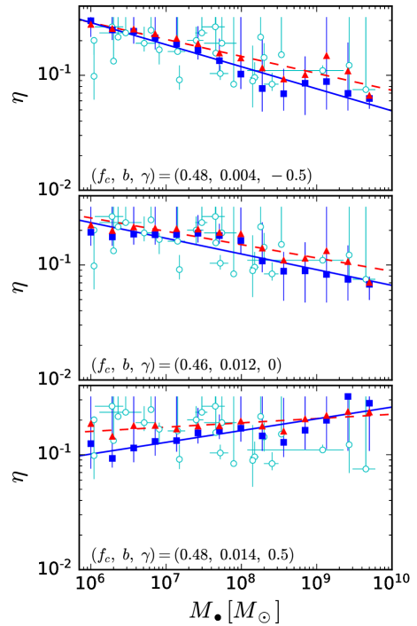
Figure 16.— Mean (red triangles) and median (blue squares) radiative efficiencies for the mock AGNs in different MBH mass bins. The mock AGN samples are obtained from those models with the largest $P_{\rm KS}$ value for the cases of $\gamma=-0.5,0$, and $0.5$, i.e., $(f_{\rm c},\ b,\ \gamma)=(0.48,\ 0.004,\ -0.5)$ (top panel), $(0.46,\ 0.012,\ 0)$ (middle panel), and $(0.48,\ 0.014,\ 0.5)$ (bottom panel) (as shown by the black dots in the left, middle, and right panels of Fig. 8), respectively. Cyan circles show the radiative efficiency of individual sources with spin measurements and they are directly converted from the spin measurements assuming the standard thin disc accretion model. The blue solid (red dashed) lines are the best linear fits to the blue squares (red triangles) in each panel, and the blue error bars represent the 16$th$ and 84$th$ percentiles.

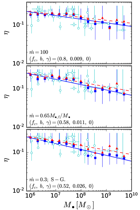
Figure 17.— Legends similar to Fig. 16, but the mock AGN samples are obtained from those models with the largest $P_{\rm KS}$ value for the case with $\dot{m}=100$ (top panel), $\dot{M}_{\rm acc}\propto\sigma^{4}$ (middle panel), and $\dot{m}=0.3$ with consideration of the self-gravity of discs in the chaotic-accretion phase.

Table 2Best parameters to fit the binned mean and median efficiencies with $\log\eta=\eta_{8}+\zeta\log(M_{\bullet}/10^{8}M_{\odot})$.

$\eta_{8,\rm mean}$	$\zeta_{\rm mean}$	$\eta_{8,\rm med}$	$\zeta_{\rm med}$	model parameters
				coherent phase ($\dot{m}$)	chaotic phase $(f_{\rm c},b,\gamma)$
$-0.84\pm 0.14$	$-0.15\pm 0.02$	$-0.93\pm 0.13$	$-0.20\pm 0.02$	$0.3$	$(0.48,0.004,-0.5)$
$-0.82\pm 0.13$	$-0.12\pm 0.02$	$-0.90\pm 0.14$	$-0.14\pm 0.02$	$0.3$	$(0.46,0.012,0)$
$-0.72\pm 0.08$	$0.04\pm 0.01$	$-0.79\pm 0.15$	$0.10\pm 0.02$	$0.3$	$(0.48,0.014,0.5)$
$-0.82\pm 0.13$	$-0.12\pm 0.02$	$-0.92\pm 0.12$	$-0.15\pm 0.01$	$0.3$	$(0.52,0.026,0),$ self-gravitating
$-0.80\pm 0.14$	$-0.08\pm 0.02$	$-0.84\pm 0.11$	$-0.09\pm 0.01$	$100$	$(0.80,0.009,0)$
$-0.83\pm 0.13$	$-0.12\pm 0.02$	$-0.89\pm 0.12$	$-0.14\pm 0.01$	$0.65\frac{M_{\bullet,\rm f}}{M_{\bullet}}$	$(0.58,0.011,0)$

The mock samples (in Fig. 8) that match the observations best are selected from the thin disc accretion stage, and thus the radiative efficiency of each MBH in those samples can be directly estimated from the MBH spin. We also calculate the mean and median efficiencies in each mass bin according to the mock samples obtained for the cases with $\gamma=-0.5$, $0$, and $0.5$, respectively (see Fig. 16). We use a simple power-law model to fit the possible relation, if any, between efficiency and MBH mass, i.e.,

$$\log\eta=\eta_{8}+\zeta\log(M_{\bullet}/10^{8}M_{\odot}),$$ (7)

and the best-fit parameters $\eta_{8}$ and $\zeta$ are listed in Table 2. For all those three $\gamma$ cases, it appears that a weak correlation exists between the mean (or median) efficiency and the MBH mass, i.e., $\eta\propto M^{\zeta}_{\bullet}$ with $|\zeta|<0.2$. For other models, i.e., with $\dot{m}=100$ or $\dot{M}_{\rm acc}\propto M_{\bullet,\rm f}$ at the coherent-accretion phase, or with self-gravitated disc considered, we plot the efficiency-mass relation in Figure 17 and list the best-fit parameters to this relation in Table 2.

Almost all those models result in a weak anti-correlation between efficiency and mass, except that the model with $\gamma=0.5$ results in almost no correlation. The result that the efficiency declines with the MBH mass is in contradiction with the positive correlation found by Davis & Laor (2011), i.e., $\eta\propto M_{\bullet}^{0.5}$. However, we note here that the correlation between $\eta$ and $M_{\bullet}$ found in Davis & Laor (2011) can be due to selection biases as pointed out in Wu et al. (2013) (see also Raimundo et al. 2012). It is also possible that the sample of the current spin measurements is heterogeneous and biased from the parent sample as further detailed in Section 4.6.

The mean efficiencies above are estimated from the mock samples by averaging over a number of mock MBHs within each mass bin. We may also estimate the mean accreted-mass-weighted efficiency ($\left<\eta\right>_{\rm m}$) for the whole accretion process of all mock MBHs, by considering the number density of MBHs with different masses. The mean efficiency is also mostly contributed by MBHs with mass around $10^{8}M_{\odot}$ as they dominate the MBH mass density. For the model with $(f_{\rm c},\ b,\ \gamma)=(0.46,\ 0.012,\ 0)$, we obtain $\left<\eta\right>_{\rm m}=0.13$. For those models with $(f_{\rm c},\ b,\ \gamma)=(0.48,\ 0.004,\ -0.5)$, $(0.48,\ 0.014,\ 0.5)$, the model considering disc self-gravity with $(f_{\rm c},\ b,\ \gamma)=(0.52,\ 0.026,\ 0)$, the model considering super-Eddington accretion ($\dot{m}=100$) in the coherent accretion phase $(f_{\rm c},\ b,\ \gamma)=(0.80,\ 0.009,\ 0)$, and the model with an upper limit on the accretion rate according to Levinson & Nakar (2018) with $(f_{\rm c},\ b,\ \gamma)=(0.58,\ 0.011,\ 0)$, we obtain $\left<\eta\right>_{\rm m}=0.15$, $0.09$, $0.12$, $0.05$, and $0.11$, respectively. For most of those models, the resulting value of $\left<\eta\right>_{\rm m}$ is consistent with the global constraint ($\sim 0.09-0.12$) obtained by comparing the local MBH mass density with the accreted MBH mass density via AGNs and QSOs in a number of references (e.g., Yu & Tremaine 2002, and references therein; Elvis et al. 2002, and references therein; Marconi et al. 2004, and references therein; Shankar et al. 2004, 2009, and references therein; Raimundo & Fabian 2009, and references therein; Raimundo et al. 2012, and references therein; Zhang et al. 2012, and references therein; Zhang & Lu 2017, and references therein). One may also note that a few recent works obtained a smaller mean efficiency of $\sim 0.05-0.06$ (e.g., Shankar et al., 2013; Ueda et al., 2014), which might be caused by adopting a higher local MBH mass density. However, if one considers the sample bias when estimating the local MBH density via different scaling relations, i.e., $M_{\bullet}-\sigma$ and $M_{\bullet}-L$ relations (e.g., Bernardi et al., 2007; Shankar et al., 2016), the value $\sim 0.05-0.06$ might be an underestimate and not necessarily contradict with the mean efficiency obtained from those models without assuming super-Eddington accretion. The mean value of the radiative efficiency ($\sim 0.05$) resulting from the model setting a super-Eddington accretion rate of $\dot{m}=100$ in the coherent-accretion phase, although consistent with the estimates by Shankar et al. (2013) and Ueda et al. (2014), seems lower than the global constraints obtained by most authors. With more measurements on MBH spins in the future, it would be possible to constrain whether most MBHs experienced a significant super-Eddington accretion by combining the estimate of mean efficiency through an independent method.

4.5. Possible cosmic evolution of MBH spins?

The two-phase model constrained above suggests that low mass MBHs spin faster than high mass ones as a combined effect of two factors: 1) the de-spin due to the late stage chaotic accretion, and 2) the more efficient de-spin of those MBHs with $M_{\bullet}\gtrsim 10^{8}M_{\odot}$ in the chaotic accretion phase. Although the cosmic evolution of MBHs is not considered in the above calculations, the two-phase model may imply a cosmic spin evolution of the active MBH population. A more comprehensive model should include both the MBH spin and mass evolution in the co-evolution model for MBHs and galaxies (see Volonteri et al., 2005; Berti & Volonteri, 2008; Dubois et al., 2014a, b; Sesana et al., 2014), though the details of the fueling to MBHs are still not well understood. With upcoming spin measurements and better determined spin distribution, it is possible to combine the constraints on the assembly history of MBHs with the co-evolution model for MBHs and galaxies to investigate the cosmic evolution of the spins of MBHs as a population. In such a cosmological evolution model of MBHs, the clustering of active MBHs can be used to put strong constraints on the lifetime and evolution of accretion histories (e.g., Aversa et al., 2015). For example, if the accretion rate is too high, with an extremely large $\dot{m}$, and the lifetime of QSOs is too short, the inferred clustering would be too low to be consistent with the observational one; if the lifetime is too long, the inferred clustering would be too high to be consistent with the observation. Therefore, the clustering of active MBHs can also put further constraint on MBH spins because larger spins mean longer lifetime in order to fit the observationally determined QSO luminosity functions.

4.6. AGN sample with spin measurements

Those models with largest $P_{\rm KS}$ value all result in a non-negligible fraction of MBHs with negative spins. In the reference model [$(f_{\rm c},b,\gamma)=(0.46,0.012,0)$; shown in the middle panel of Fig. 8], for example, about $5.5\%$ of the mock objects are accreting via discs counter-rotating around their central MBHs. However, all the active MBHs in Table 1 have positive spins. One reason might be the small sample size of MBHs with spin measurements. In Table 1, $18$ objects have masses in the range from $10^{6}$ to $10^{8}M_{\odot}$, and the other $9$ have masses $>10^{8}M_{\odot}$. The fraction of negative spins resulting from the reference model is $1.5\%$ in the mass range $10^{6}-10^{8}M_{\odot}$, while it increases to $\sim 13.3\%$ for $>10^{8}M_{\odot}$ MBHs. According to the Poisson statistics, the probability to observe $k$ counter-rotating MBHs is given by $P(k)=\frac{e^{-\lambda}\lambda^{k}}{k!}$, if the expected number of counter-rotating MBHs is $\lambda$, where $k=0,1,2,...$. Then the probability of non-detection of negative spins among the $18$ objects with mass of $10^{6}-10^{8}M_{\odot}$ is quite high, i.e., $P(0)\simeq 0.76$, and the probability not to detect negative spins among the $9$ objects with mass $>10^{8}M_{\odot}$ is $P(0)\simeq 0.30$ (see Fig. 9). Therefore, non-detection of a negative spin appears not a serious problem as the size of the currently available spin sample is small. One may note that a recent spin measurement of 1H 1934-063, a narrow-line Seyfert 1 galaxy, gives $a<0.1$ (Frederick et al., 2018), which seems to be consistent with a non-spinning or even a counter-rotating MBH. However, this measurement only gives an upper limit and is not included in the above 2D-KS tests in which cumulative spin distributions (with spin smaller than a value of $a$) were considered.

The other reason might be that the sample listed in Table 1 is incomplete. Though it is still not clear whether the sample is biased or not, some authors (e.g., Brenneman, 2013) indeed pointed out that it is more likely to detect high spin MBHs by applying the X-ray reflection spectroscopy method. The inner disc radius of a high spin and/or prograde system is smaller than that of a low spin and/or retrograde system, and thus relativistic effects are more prominent. High signal-to-noise ratio spectroscopy is also needed in order to measure the spin. This means the targeted object should be bright enough, which may be easier satisfied for those MBHs radiating efficiently with high spins.

The limited sample size and the possible bias present caveats in constraining the MBH growth history described above. Future X-ray telescopes, such as Athena, Hitomi, LOFT, and eXTP, may accurately measure several hundred or more MBH spins without or with less bias, and thus may provide stronger constraints on the growth history of MBHs.

There are only three MBHs in Table 1 having mass $M_{\bullet}>10^{9}M_{\odot}$, i.e., H 1821+643 with $a>0.4$, Q 2237+305 with $a=0.74^{+0.06}_{-0.03}$, and SDSS J094533.99+100950.1 with $a=0.8^{+0.2}_{-0.5}$. It is important to check whether the constraints obtained above are significantly affected by these three sources. We therefore exclude these three sources and repeat the calculation, and we find that the obtained constraints do not differ much from the above results. It is worth noting that two important factors lead to the constraints on the MBH accretion history. First, the spin distribution for MBHs with mass ranging from $10^{6}-10^{8}M_{\odot}$ in Table 1 is narrow and the majority of the samples have spins $\gtrsim 0.8$, which suggest that the disc mass in the chaotic-accretion phase, if any, cannot be too small. If it is too small (e.g., $b<0.003$), then the spin distribution at this mass range cannot be that narrow. We have checked that if only using those spin observations for MBHs with mass $<10^{8}M_{\odot}$, we still obtain similar constraints on $(f_{\rm c},b)$, though the values of the largest $P_{\rm KS}$ does decrease somehow and the constraints become slightly less strong. Second, about one third of the observed objects have masses $M_{\bullet}\gtrsim 10^{8}M_{\odot}$ and spins broadly distributed, i.e. $a\sim 0.5-1$. The existence of these objects indicates the amount of the MBH mass coming from chaotic-accretion phase and suggests that chaotic accretion phase is significant for the MBH growth and spin evolution.

5. Conclusions

In this paper, we study the spin evolution of MBHs under the assumption that MBHs experienced two accretion phases, with an initial phase of coherent-accretion via either the standard thin disc or super-Eddington accretion, followed by a second phase of chaotic accretion via the standard thin disc. As illustrated by many authors in previous works, if the first phase dominates the MBH growth, then most MBHs should be quickly spun up, to close to the maximum spin value (e.g., $\sim 0.998$); if the chaotic-accretion phase is important, MBHs with mass $\gtrsim 10^{8}M_{\odot}$ may be significantly spun down at their late growth stage. If the chaotic accretion phase dominates the growth of MBHs and the coherent accretion is negligible, we further find that the spins of those MBHs may quickly reach a quasi-equilibrium state at their early growth stage and this state ends up when the disc size becomes smaller than the warp radius of non-equatorial disc(s). The value of the spin at the quasi-equilibrium state is roughly determined by the mean ratio of the disc mass to the MBH mass in the chaotic-accretion phase, i.e., the smaller this ratio, the smaller the equilibrium spin value. Therefore, the spin distribution of those MBHs with mass $\sim 10^{6}-10^{8}M_{\odot}$ is mainly determined by the mean (or distribution of) ratio of the disc mass to the MBH mass in chaotic accretion episodes.

Utilizing the spin evolutionary models studied in this paper, we further investigate how the constraints on the MBH growth histories can be obtained from the latest available spin measurements via the X-ray reflection spectroscopy. We find that MBHs should experience a chaotic-accretion phase with many accretion episodes, and on average the mass accreted within each episode is roughly $1$-$2$ percent of the MBH mass or less. The total amount of mass accreted in the chaotic phase is at least $5-20$ percent of the final MBH mass. MBHs with masses $\gtrsim 10^{8}M_{\odot}$ appear to have intermediate-to-high spins ($\sim 0.5-1$), while MBHs with lower masses ($\sim 10^{6}-10^{8}M_{\odot}$) appear to have higher spins ($\gtrsim 0.8$). On average, the radiative efficiencies of those active MBHs appear to slightly decrease with increasing MBH masses. This indicates that the correlation between the radiative efficiency and the MBH mass, if any, is weak. The mean radiative efficiency of active MBHs is $\sim 0.09-0.15$, consistent with the global constraints by comparing the accreted mass density with the local MBH mass density.

Appendix A Inner boundary of the standard thin accretion disc around an MBH

For an MBH accreting with $f_{\rm Edd}\lesssim 1$, the accretion disc is assumed to be geometrically thin, optically thick, and described by the standard thin disc model (e.g., Shakura & Sunyaev, 1973; Novikov & Thorne, 1973). Then the inner boundary of the disc is (Bardeen et al., 1972)

$$R_{\rm in}=R_{\rm ISCO}={3+Z_{2}\mp[(3-Z_{1})(3+Z_{1}+2Z_{2})]^{1/2}},$$

(A1)

with

$$Z_{1} = 1+(1-a^{2})^{1/3}[(1+a)^{1/3}+(1-a)^{1/3}],$$ (A2)

$$Z_{2} = (3a^{2}+Z_{1}^{2})^{1/2},$$ (A3)

where $a=\left|a\right|$ when the disc is prograde rotating, $a=-\left|a\right|$ when the disc is retrograde rotating, the upper (lower) case of ‘$\mp$’ (or ‘$\pm$’) sign represents the prograde (retrograde) orbit, and the same afterwards.

The general form of the specific energy $E$ and angular momentum $\Phi$ as a function of radius $r$ (in unit of $r_{\rm g}=GM_{\bullet}/c^{2}$) of a circular orbit are given by (Bardeen et al., 1972)

$$E(r)=\frac{r^{3/2}-2r^{1/2}+a}{r^{3/4}(r^{3/2}-3r^{1/2}+2a)^{1/2}},$$ (A4)

$$\Phi(r)=\pm\frac{(r^{2}-2ar^{1/2}+a^{2})}{r^{3/4}(r^{3/2}-3r^{1/2}+2a)^{1/2}}.$$ (A5)

Then the specific energy and angular momentum at $R_{\rm ISCO}$ can be obtained by setting $r=R_{\rm ISCO}$.

Appendix B inner disc boundary of thick discs

For super-Eddington accretion, we apply the logarithmic dependence of Eddington ratio on the accretion rate given by Mineshige et al. (2000), i.e.,

$$f_{\rm Edd}=\left\{\begin{array}[]{l l}2[1+\ln(8\dot{m}/25)],&\mbox{if}\,\ \dot{m}>25/8\\ 16\dot{m}/25,&\mbox{otherwise}.\end{array}\right.$$ (B3)

Note that the above formula looks different from that in the reference paper, simply because the $\dot{M}_{\rm Edd}$ defined here is $16$ times larger than that in Mineshige et al. (2000). Then according to $\eta=f_{\rm Edd}/(16\dot{m})$, we have

$$\eta=\left\{\begin{array}[]{l l}[1+\ln(8\dot{m}/25)]/(8\dot{m}),&\mbox{if}\,\ \dot{m}>25/8\\ 1/25,&\mbox{otherwise}.\end{array}\right.$$ (B6)

For thick disc accretion, we have $R_{\rm mb}<R_{\rm in}<R_{\rm ISCO}$ (Kozłowski et al., 1978; Jaroszynski et al., 1980), where $R_{\rm mb}=2-a+2(1-a)^{1/2}$ is the marginally bound orbit. In order to calculate the energy and angular momentum brought into the central MBH through the inner boundary of the accretion disc, we approximately estimate $R_{\rm in}$ according to the following procedures. (i) For a given $\dot{m}$, $\eta$ is estimated from Equation (B6), and $E(R_{\rm in})=1-\eta$ assuming that the kinetic energy output is negligible. (ii) According to Equation (A4), $E(r)$ can be obtained for any given radius $r$ provided known spin $a$, and thus an array of $r$ and $E(r)$ can be obtained. (iii) With the $E(R_{\rm in})$ derived in step (i), $R_{\rm in}$ is then obtained by interpolation of the array, and with Eq. (A5) the specific angular momentum at $R_{\rm in}$ can be obtained.

Appendix C properties of accretion disc in chaotic phase

The disc in the chaotic phase is assumed to be described by the thin disc model (Shakura & Sunyaev, 1973), and the properties of the disc has been studied in detail by Perego et al. (2009) and Dotti et al. (2013). Here we only give a brief summary of them.

We assume a power-law profile of radial and vertical shear viscosity, i.e., $\nu_{1}\propto R^{3/4}$ and $\nu_{2}\propto R^{3/4}$. The $\alpha$-prescription is applied and $\alpha=0.09$ for radial viscosity. Choosing a different $\alpha$ does not significantly affect our results. For a disc with mass $M_{\rm disc}=M_{\rm cl}=bM^{\gamma+1}_{\bullet}$ (Eq. 4), the surface density profile is given by the outer solution of the standard thin disc model, i.e.,

$$\Sigma(R)=\Sigma_{0}(R/2r_{\rm g})^{-3/4},$$ (C1)

where $r_{\rm g}=GM_{\bullet}/c^{2}$ is the gravitational radius and

$$\Sigma_{0}=4\times 10^{7}\ \alpha^{-4/5}_{0.1}M^{1/5}_{{\bullet},6}\left(\frac{f_{\rm Edd}}{\eta_{0.1}}\right)^{7/10}{\rm g\ cm^{-2}}.$$ (C2)

Here $\alpha_{0.1}=\alpha/0.1$, $\eta_{0.1}=\eta/0.1$, and $M_{{\bullet},6}$ is MBH mass in unit of $10^{6}M_{\odot}$. The disc size can then be derived as

$$R_{{\rm disc}}\approx 10^{5}\left(\frac{b}{0.01}\right)^{4/5}\alpha^{16/25}_{0.1}M^{-24/25}_{{\bullet},6}\left(\frac{f_{\rm Edd}}{\eta_{0.1}}\right)^{-14/25}r_{\rm g}.$$ (C3)

In the first order approximation, the disc angular momentum per unit area is given by

$$L(R)\approx\frac{\dot{M}}{3\pi\nu_{1}}\sqrt{GM_{\bullet}R}.$$ (C4)

Then the angular momentum of the whole disc can be derived by integrating $L(R)$ over all annuli and set $R=R_{\rm disc}$, which yields

$$J_{\rm disc}\propto\dot{M}\sqrt{GM_{\bullet}}R^{7/4}_{{\rm disc}}.$$ (C5)

The disc-to-MBH angular momentum ratio, which governs the MBH spin evolution, can then be expressed as

$$\frac{J_{\rm disc}}{J_{\bullet}}\approx 3\ \left(\frac{b}{0.01}\right)^{7/5}\alpha^{8/25}_{0.1}M^{-12/25}_{{\bullet},6}\left(\frac{f_{\rm Edd}}{\eta_{0.1}}\right)^{-7/25}a^{-1}.$$ (C6)

The general misalignment between the angular momenta of disc and MBH spin induces deformation in the disc (Bardeen & Petterson, 1975), which is maximally warped at around

$$R_{\rm warp}\approx 1000\ \alpha^{24/35}_{0.1}f^{-4/7}_{\nu_{2}}M^{4/35}_{{\bullet},6}\left(\frac{f_{\rm Edd}}{\eta_{0.1}}\right)^{-6/35}a^{4/7}r_{\rm g},$$ (C7)

where $f_{\nu_{2}}=2\alpha^{2}\nu_{2}/\nu_{1}$ is a coefficient describing non-linear effect ant $f_{\nu_{2}}=0.6$ according to simulation results (see Lodato & Pringle, 2007; Perego et al., 2009, for details). The equality $R_{\rm warp}=R_{\rm disc}$ defines a critical MBH mass of

$$M^{\rm crit}_{{\bullet}}\approx 10^{7}M_{\odot}\ \left(\frac{M_{\rm disc}}{10^{4}M_{\odot}}\right)^{35/82}\alpha^{-1/41}_{0.1}a^{-25/82}\left(\frac{f_{\rm Edd}}{\eta_{0.1}}\right)^{-17/82}f^{25/82}_{\nu_{2}}.$$ (C8)

As for the self-gravitated disc, the criterion for disc stability is given by the Toomre-$Q$ parameter with $Q\sim\Omega c_{s}/\pi G\Sigma$ (see Binney & Tremaine, 2008), where $\Omega$ is the angular velocity and $c_{s}$ is the sound speed. The critical case of $Q=1$ yields a maximum disc radius

$$R_{{\rm disc},{\rm sg}}\approx 2\times 10^{5}\ \alpha^{28/45}_{0.1}M^{-52/45}_{{\bullet},6}\left(\frac{f_{\rm Edd}}{\eta_{0.1}}\right)^{-22/45}r_{\rm g},$$ (C9)

which implies a possible upper limit on the disc mass, i.e.,

$$M_{\rm sg}\approx 2\times 10^{4}\ \alpha^{-1/45}_{0.1}\left(\frac{f_{\rm Edd}}{\eta_{0.1}}\right)^{4/45}M^{34/45}_{{\bullet},6}M_{\sun}.$$ (C10)

References

- Abramowicz et al. (1988) Abramowicz, M. A., Czerny, B., Lasota, J. P., & Szuszkiewicz, E. 1988, ApJ, 332, 646
- Agís-González et al. (2014) Agís-González, B., Miniutti, G., Kara, E., et al. 2014, MNRAS, 443, 2862
- Assef et al. (2011) Assef, R. J., Denney, K. D., Kochanek, C. S., et al. 2011, ApJ, 742, 93
- Aversa et al. (2015) Aversa, R., Lapi, A., de Zotti, G., Shankar, F., & Danese, L. 2015, ApJ, 810, 74
- Bañados et al. (2018) Bañados, E., Venemans, B. P., Mazzucchelli, C., et al. 2018, Nature, 553, 473
- Bardeen & Petterson (1975) Bardeen, J. M., & Petterson, J. A. 1975, ApJ, 195, 65
- Bardeen et al. (1972) Bardeen, J. M., Press, W. H., & Teukolsky, S. A. 1972, ApJ, 178, 347
- Bennert et al. (2011) Bennert, V. N., Auger, M. W., Treu, T., Woo, J.-H., & Malkan, M. A. 2011, ApJ, 726, 59
- Bentz et al. (2006) Bentz, M. C., Denney, K. D., Cackett, E. M., et al. 2006, ApJ, 651, 775
- Bernardi et al. (2007) Bernardi, M., Sheth, R. K., Tundo, E., & Hyde, B. 2007, ApJ, 660, 267
- Berti & Volonteri (2008) Berti, E., Volonteri, M. 2008, ApJ, 684, 822
- Binney & Tremaine (2008) Binney, J., & Tremaine, S. 2008, Galactic Dynamics: Second Edition, by James Binney and Scott Tremaine. ISBN 978-0-691-13026-2 (HB). Published by Princeton University Press, Princeton, NJ USA, 2008
- Brenneman (2013) Brenneman, L. 2013, AcPol, 53, 652
- Brenneman & Reynolds (2006) Brenneman, L. W., & Reynolds, C. S. 2006, ApJ, 652, 1028
- Brenneman et al. (2011) Brenneman, L. W., Reynolds, C. S., Nowak, M. A., et al. 2011, ApJ, 736, 103
- Centrella et al. (2010) Centrella, J., Baker, J. G., Kelly, B. J., & van Meter, J. R. 2010, Reviews of Modern Physics, 82, 3069
- Czerny et al. (2011) Czerny, B., Hryniewicz, K., Nikołajuk, M., & Sadowski, A. 2011, MNRAS, 415, 2942
- Davis & Laor (2011) Davis, S. W., & Laor, A. 2011, ApJ, 728, 98
- Dotti et al. (2013) Dotti, M., Colpi, M., Pallini, S., et al. 2013, ApJ, 762, 68
- Du et al. (2015) Du, P., Hu, C., Lu, K.-X., et al. 2015, ApJ, 806, 22
- Dubois et al. (2014a) Dubois, Y., Volonteri, M., Silk, J., Devriendt, J., & Slyz, A. 2014a, MNRAS, 440, 2333
- Dubois et al. (2014b) Dubois, Y., Volonteri, M., & Silk, J. 2014b, MNRAS, 440, 1590
- Elvis et al. (2002) Elvis, M., Risaliti, G., & Zamorani, G. 2002, ApJ, 565, L75
- Fabian et al. (2013) Fabian, A. C., Kara, E., Walton, D. J., et al. 2013, MNRAS, 429, 2917
- Fabian et al. (1989) Fabian, A. C., Rees, M. J., Stella, L., & White, N. E. 1989, MNRAS, 238, 729
- Ferrarese et al. (2000) Ferrarese, L., & Merritt, D. 2000, ApJ, 539, L9
- Fiacconi et al. (2018) Fiacconi, D., Sijacki, D., & Pringle, J. E. 2018, MNRAS, 477, 3807
- Frederick et al. (2018) Frederick, S. E., Kara, E., Reynolds, C. S., Pinto, C., & Fabian, A. C. 2018, ApJ, 867, 67
- Gallo et al. (2011) Gallo, L. C., Miniutti, G., Miller, J. M., et al. 2011, MNRAS, 411, 607
- Gallo et al. (2015) Gallo, L. C., Wilkins, D. R., Bonson, K., et al. 2015, MNRAS, 446, 633
- Gammie et al. (2004) Gammie, C. F., Shapiro, S. L., & McKinney, J. C. 2004, ApJ, 602, 312
- Gebhardt et al. (2000) Gebhardt, K., Bender, R., Bower, G., et al. 2000, ApJ, 539, L13
- Gebhardt & Thomas (2009) Gebhardt, K., & Thomas, J. 2009, ApJ, 700, 1690
- Goodman & Tan (2004) Goodman, J., & Tan, J. C. 2004, ApJ, 608, 108
- González-Martín & Vaughan (2012) González-Martín, O., Vaughan, S. 2012, A&A, 544, A80
- Gültekin et al. (2009) Gültekin, K., Richstone, D. O., Gebhardt, K., et al. 2009, ApJ, 698, 198
- Hopkins & Hernquist (2006) Hopkins, P. F., & Hernquist, L. 2006, ApJS, 166, 1
- Hopkins et al. (2007) Hopkins, P. F., Richards, G. T., & Hernquist, L. 2007, ApJ, 654, 731
- Jaroszynski et al. (1980) Jaroszynski, M., Abramowicz, M. A., & Paczynski, B. 1980, Acta Astronomica, 30, 1
- Jiang et al. (2014) Jiang, Y-F., Stone, J. M., & Davis, S. W. 2014, ApJ, 796, 106
- Keck et al. (2015) Keck, M. L., Brenneman, L. W., Ballantyne, D. R., et al. 2015, ApJ, 806, 149
- King et al. (2005) King, A. R., Lubow, S. H., Ogilvie, G. I., & Pringle, J. E. 2005, MNRAS, 363, 49
- King & Pringle (2006) King, A. R., & Pringle, J. E. 2006, MNRAS, 373, L90
- King et al. (2008) King, A. R., Pringle, J. E., & Hofmann, J. A. 2008, MNRAS, 385, 1621
- Kolykhalov & Sunyaev (1980) Kolykhalov, P. I., & Sunyaev, R. A. 1980, SvAL, 6, 357
- Kormendy & Richstone (1995) Kormendy, J., & Richstone, D. 1995, ARA&A, 33, 581
- Kormendy & Ho (2013) Kormendy, J., & Ho, L. C. 2013, ARA&A, 51, 511
- Kozłowski et al. (1978) Kozłowski, M., Jaroszyński, M., & Abramowicz, M. A. 1978, A&A, 63, 209
- Krolik (1999) Krolik, J. H. 1999, Active galactic nuclei : from the central black hole to the galactic environment /Julian H. Krolik. Princeton, N. J. : Princeton University Press, c1999.,
- LaMassa et al. (2015) LaMassa, S. M., Cales, S., Moran, E. C., et al. 2015, ApJ, 800, 144
- Laor (1991) Laor, A. 1991, ApJ, 376, 90
- Lapi et al. (2006) Lapi, A., Shankar, F., Mao, J., et al. 2006, ApJ, 650, 42
- Lehner & Pretorius (2014) Lehner, L., & Pretorius, F. 2014, ARA&A, 52, 661
- Lense & Thirring (1918) Lense, J., & Thirring, H. 1918, Phys. Z., 19, 156
- Levinson & Nakar (2018) Levinson, A., & Nakar, E. 2018, MNRAS, 473, 2673
- Li (2012) Li, L.-X. 2012, MNRAS, 424, 1461
- Li et al. (2015) Li, Y.-R., Wang, J.-M., Cheng, C., & Qiu, J. 2015, ApJ, 804, 45
- Lodato et al. (2006) Lodata, G., & Pringle, J. E. 2006, MNRAS, 368, 1196
- Lodato & Pringle (2007) Lodato, G., & Pringle, J. E. 2007, MNRAS, 381, 1287
- Lohfink et al. (2013) Lohfink, A. M., Reynolds, C. S., Jorstad, S. G., et al. 2013, ApJ, 772, 83
- Lohfink et al. (2012) Lohfink, A. M., Reynolds, C. S., Miller, J. M., et al. 2012, ApJ, 758, 67
- Lousto et al. (2010) Lousto, C. O., Campanelli, M., Zlochower, Y., & Nakano, H. 2010, Classical and Quantum Gravity, 27, 114006
- Macchetto et al. (1997) Macchetto, F., Marconi, A., Axon, D. J., et al. 1997, ApJ, 489, 579
- Madau et al. (2014) Madau, P., Haardt, F., & Dotti, M. 2014, ApJ, 784, 38
- Magorrian et al. (1998) Magorrian, J., Tremaine, S., Richstone, D., et al. 1998, ApJ, 115, 2285
- Malizia et al. (2008) Malizia, A., Bassani, L., Bird, A. J., et al. 2008, MNRAS, 389, 1360
- Marconi et al. (2004) Marconi, A., Risaliti, G., Gilli, R., et al. 2004, MNRAS, 351, 169
- Martini (2004) Martini, P. 2004, Coevolution of Black Holes and Galaxies, 169
- Martine et al. (2007) Martin, R. G., Pringle, J. E., & Tout, C. A. 2007, MNRAS, 381, 1617
- McHardy et al. (2005) McHardy, I. M., Gunn, K. F., Uttley, P., & Goad, M. R. 2005, MNRAS, 359, 1469
- Mineshige et al. (2000) Mineshige, S., Kawaguchi, T., Takeuchi, M., & Hayashida, K. 2000, PASJ, 52, 499
- Miniutti et al. (2009) Miniutti, G., Panessa, F., De Rosa, A., et al. 2009, MNRAS, 398, 255
- Miniutti et al. (2010) Miniutti, G., Piconcelli, E., Bianchi, S., Vignali, C., & Bozzo, E. 2010, MNRAS, 401, 1315
- Moderski et al. (1998) Moderski, R., Sikora, M., & Lasota, J.-P. 1998, MNRAS, 301, 142
- Mortlock et al. (2011) Mortlock, D. J., Warren, S. J., Venemans, B. P., et al. 2011, Nature, 474, 616
- Nikołajuk et al. (2009) Nikołajuk, M., Czerny, B., & Gurynowicz, P. 2009, MNRAS, 394, 2141
- Novikov & Thorne (1973) Novikov, I. D., & Thorne, K. S. 1973, Black Holes (Les Astres Occlus), 343
- Patrick et al. (2012) Patrick, A. R., Reeves, J. N., Porquet, D., et al. 2012, MNRAS, 426, 2522
- Perego et al. (2009) Perego, A., Dotti, M., Colpi, M., & Volonteri, M. 2009, MNRAS, 399, 2249
- Peterson et al. (2004) Peterson, B. M., Ferrarese, L., Gilbert, K. M., et al. 2004, ApJ, 613, 682
- Press et al. (2007) Press, W. H., Teukolsky, S. A., Vetterling, W. T., & Flannery, B. P. 2007, Numerical recipes, 3rd edn. Cambridge Univ. Press, Cambridge, p. 762
- Raimundo & Fabian (2009) Raimundo, S. I., & Fabian, A. C. 2009, MNRAS, 396, 1217
- Raimundo et al. (2012) Raimundo, S. I., Fabian, A. C., Vasudevan, R. V., Gandhi, P., & Wu, J. 2012, MNRAS, 419, 2529
- Reis et al. (2014) Reis, R. C., Reynolds, M. T., Miller, J. M., & Walton, D. J. 2014, Nature, 507, 207
- Reynolds et al. (2014) Reynolds, C. S., Lohfink, A. M., Babul, A., et al. 2014, ApJ, 792, L41
- Reynolds (2014) Reynolds, C. S. 2014, SSRv, 183, 277
- Reynolds et al. (2014) Reynolds, M. T., Walton, D. J., Miller, J. M., & Reis, R. 2014, ApJ, 792, L19
- Risaliti et al. (2013) Risaliti, G., Harrison, F. A., Madsen, K. K., et al. 2013, Nature, 494, 449
- Risaliti et al. (2009) Risaliti, G., Miniutti, G., Elvis, M., et al. 2009, ApJ, 696, 160
- Ruan et al. (2016) Ruan, J. J., Anderson, S. F., Cales, S. L., et al. 2016, ApJ, 826, 188
- Sądowski (2009) Sądowski, A. 2009, ApJS, 183, 171
- Sądowski et al. (2011) Sądowski, A., Bursa, M., Abramowicz, M., et al. 2011, A&A, 532, 41
- Saglia et al. (2016) Saglia, R. P., Opitsch, M., Erwin, P., et al. 2016, ApJ, 818, 47
- Schulze & Wisotzki (2010) Schulze, A., & Wisotzki, L. 2010, A&A, 516, A87
- Sesana et al. (2014) Sesana, A., Barausse, E., Dotti, M., Rossi, E. M. 2014, ApJ, 794, 104
- Shakura & Sunyaev (1973) Shakura, N. I., & Sunyaev, R. A. 1973, A&A, 24, 337
- Shankar et al. (2016) Shankar, F., Bernardi, M., Sheth, R. K. 2016, MNRAS, 460, 3119
- Shankar et al. (2004) Shankar, F., Salucci, P., Granato, G. L., De Zotti, G., & Danese, L. 2004, MNRAS, 354, 1020
- Shankar et al. (2009) Shankar, F., Weinberg, D. H., & Miralda-Escudé, J. 2009, ApJ, 690, 20
- Shankar et al. (2013) Shankar, F., Weinberg, D. H., & Miralda-Escudé, J. 2009, MNRAS, 428, 421
- Shen et al. (2008) Shen, Y., Greene, J. E., Strauss, M. A., Richards, G. T., & Schneider, D. P. 2008, ApJ, 680, 169
- Shen (2009) Shen, Y. 2009, ApJ, 704, 89
- Shen et al. (2011) Shen, Y., Richards, G. T., Strauss, M. A., et al. 2011, ApJS, 194, 45
- Sluse et al. (2012) Sluse, D., Hutsemékers, D., Courbin, F., Meylan, G., & Wambsganss, J. 2012, A&A, 544, A62
- Sołtan (1982) Sołtan, A. 1982, MNRAS, 200, 115
- Suh et al. (2015) Suh, H., Hasinger, G., Steinhardt, C., Silverman, J. D., & Schramm, M. 2015, ApJ, 815, 129
- Sun et al. (2017) Sun, S., Guainazzi, M., Ni, Q., et al. 2017, arXiv:1704.03716
- Tanaka et al. (1995) Tanaka, Y., Nandra, K., Fabian, A. C., et al. 1995, Nature, 375, 659
- Tan et al. (2012) Tan, Y., Wang, J. X., Shu, X. W., & Zhou, Y. 2012, ApJ, 747, L11
- Thorne (1974) Thorne, K. S. 1974, ApJ, 191, 507
- Tremaine et al. (2002) Tremaine, S., Gebhardt, K., Bender, R., et al. 2002, ApJ, 574, 740
- Ueda et al. (2014) Ueda, Y., Akiyama, M., Hasinger, G., et al. 2014, ApJ, 786, 104
- Vasudevan et al. (2016) Vasudevan, R. V., Fabian, A. C., Reynolds, C. S., et al. 2016, MNRAS, 458, 2012
- Vestergaard & Peterson (2006) Vestergaard, M., & Peterson, B. M. 2006, ApJ, 641, 689
- Volonteri et al. (2013) Volonteri, M., Sikora, M., Lasota, J.-P., & Merloni, A. 2013, ApJ, 775, 94
- Volonteri et al. (2005) Volonteri, M., Madau, P., Quataert, E., & Rees, M. J. 2005, ApJ, 620, 69
- Walton et al. (2013) Walton, D. J., Nardini, E., Fabian, A. C., Gallo, L. C., & Reis, R. C. 2013, MNRAS, 428, 2901
- Wu et al. (2013) Wu, S., Lu, Y., Zhang, F., & Lu, Y. 2013, MNRAS, 436, 3271
- Wu et al. (2015) Wu, X-B., Wang, F., Fan, X., et al. 2015, Nature, 518, 512
- Yu & Lu (2004) Yu, Q., & Lu, Y. 2004, ApJ, 602, 603
- Yu & Lu (2008) Yu, Q., & Lu, Y. 2008, ApJ, 689, 732
- Yu et al. (2005) Yu, Q., Lu, Y., & Kauffmann, G. 2005, ApJ, 634, 901
- Yu & Tremaine (2002) Yu, Q., & Tremaine, S. 2002, MNRAS, 335, 965
- Zhang & Lu (2017) Zhang, X., & Lu, Y. 2017, Science China Physics, Mechanics, and Astronomy, 60, 109511
- Zhang et al. (2012) Zhang, X., Lu, Y., & Yu, Q. 2012, ApJ, 761, 5
- Zhang et al. (2018) Zhang, X., Lu, Y., & Liu, Z. 2018, submitted to ApJ
- Zhou & Wang (2005) Zhou, X.-L., & Wang, J.-M. 2005, ApJ, 618, L83
- Zoghbi et al. (2010) Zoghbi, A., Fabian, A. C., Uttley, P., et al. 2010, MNRAS, 401, 2419