Solving large-scale interior eigenvalue problems to investigate the vibrational properties of the boson peak regime in amorphous materials

Abstract

Amorphous solids, like metallic glasses, exhibit an excess of low frequency vibrational states reflecting the break-up of sound due to the strong structural disorder inherent to these materials. Referred to as the boson peak regime of frequencies, how the corresponding eigenmodes relate to the underlying atomic-scale disorder remains an active research topic. In this paper we investigate the use of a polynomial filtered eigensolver for the computation and study of low frequency eigenmodes of a Hessian matrix located in a specific interval close to the boson peak regime. A distributed-memory parallel implementation of a polynomial filtered eigensolver is presented. Our implementation, based on the Trilinos framework, is then applied to Hessian matrices of different atomistic bulk metallic glass structures derived from molecular dynamics simulations for the computation of eigenmodes close to the boson peak. In addition, we demonstrate the parallel scalability of our implementation on multicore nodes. Our resulting calculations successfully concur with previous atomistic results, and additionally demonstrate a broad cross-over of boson peak frequencies within which sound is seen to break-up.

1 Introduction

In amorphous materials, such as structural glass, sound waves have a meaning only within a finite range of wavelengths. At long wavelengths, the heterogeneity of the amorphous structure self averages and an elastic continuum emerges. In this regime, sound is well defined via a linear dispersion characterized by a velocity set by the continuum’s isotropic elastic constants. However, as the wavelength reduces, the structural heterogeneity of the glass is increasingly probed, resulting in a broadening of a sound mode’s frequency spectrum. When this broadening becomes comparable to the frequency of the sound wave (the Ioffe–Regel limit), sound loses its traditional meaning as a propagating plane wave. In this frequency range, the density of vibrational modes allowed by the solid is enhanced (the boson peak), also suggesting a transition from propagating to more localized or quasi-localized non-propagating modes. The precise nature of this transition (or cross-over behavior), and its relation to glass structure, remains an active area of research [47, 33, 36, 25, 14, 32, 24, 34, 10, 22].

One avenue in which this phenomenon may be studied is via the molecular dynamics simulation technique – a particle trajectory method able to produce structural glasses with atomic scale resolution. Indeed computer generated amorphous structures may be generated in which the force on each atom is identically zero. The harmonic vibrational properties of this stable structure, which is at a local minimum of the cohesive energy landscape, may then be investigated through the local quadratic curvature of this energy surface. This is done by realizing that the leading order deviation in energy of a stable configuration (defined by the $N$ atomic positions, $\bm{r}_{i}$) may be expressed as the quadratic form

$$E\left(\left\{\bm{r}_{i}+\bm{q}_{i}\right\}\right)=E\left(\left\{\bm{r}_{i}\right\}\right)+\frac{1}{2}\sum_{i,j=1}^{N}\bm{q}_{ij}\bm{\Delta}_{ij}\bm{q}_{ij},$$ (1)

where $\bm{q}_{ij}=\bm{q}_{i}-\bm{q}_{j}$, and $\bm{q}_{i}$ is the deviation of the $i$th atom from its position $\bm{r}_{i}$. In the above, $\bm{\Delta}_{ij}$ is therefore the second derivative with respect to the bond-length deviations $\bm{q}_{ij}$. $\bm{\Delta}_{ij}$ is a symmetric $3\times 3$ matrix. The quadratic energy term then defines a linear restoring force for such deviations, and an equation of motion for the $\left\{\bm{q}_{i}\right\}$ coordinates whose secular form equals

$$\sum_{j=1}^{N}\left(\delta_{ij}(\omega_{n})^{2}-\bm{H}_{ij}\right)\bm{q}_{n,j}=0,\qquad 1\leq n\leq N,$$ (2)

where $\bm{H}_{ij}=\bm{\Delta}_{ij}/\sqrt{m_{i}m_{j}}$, $m_{i}$ is the mass of the $i$th atom, and $\omega_{n}$ is the frequency of the $n$th vibrational eigenmode $\bm{q}_{n,i}$. The energy function, $E\left(\left\{\bm{r}_{i}\right\}\right)$, is usually determined through an empirical force model which is short range (for metallic and covalent systems), i.e., which spans a few atomic distances and results in a sparse matrix $\bm{H}$.

Therefore, in order to calculate the vibrational frequencies, $\omega_{n}=\sqrt{\lambda_{n}}$, we have to solve a real symmetric eigenvalue problem

$$\bm{H}\bm{q}=\lambda\bm{q},\qquad\bm{H}\in{\mathbb{R}}^{3N\times 3N},\quad\bm{q}\in{\mathbb{R}}^{3N}.$$ (3)

The regime of frequencies relevant to sound waves and the boson peak regime are at the lower end of the eigenvalue spectrum. Early simulation work had often considered system sizes in the range of several thousand atoms, and more recent work has considered system sizes up to several hundred thousand atoms. Contemporary understanding of the frequency regime of the boson peak suggests the relevant length scales correspond to those of elastic heterogeneities – a length scale which is at least an order of magnitude larger than an inter-atomic distance. Thus, if one wishes to study the transition from well defined propagating sound waves to their break up, larger system sizes will be needed spanning values of $N$ up to several tens if not hundreds of millions of atoms. For such large system sizes, the boson peak eigenvalue regime is no longer an extremal eigenvalue problem, since there will now be a significant interval of (lower) eigenvalues describing the allowed sound waves. This fact motivates the development of eigensolver methods which are able to focus on a finite interval of eigenvalues in the interior of the spectrum of $\bm{H}$ and their eigenvectors.

The shift-and-invert Lanczos (SI-Lanczos) algorithm is the method of choice for computing interior eigenvalues and corresponding eigenvectors of a symmetric or Hermitian matrix $\bm{H}$ close to some target $\tau$. However, the SI-Lanczos algorithm needs the factorization of $\bm{H}-\tau\bm{I}$ which is not feasible here for its excessive memory requirements. For such cases, the Jacobi–Davidson methods have been developed [40, 41, 39]. To be efficient, they however need an effective preconditioner to solve the so-called correction equation, which usually entails its factorization [3]. In an earlier study [31], we were not able to identify such preconditioners for (3).

In this work we investigate a technique, known as spectral filtering, for solving eigenvalue problems that obviates factorizations altogether [37, 38, 18, 19]. Spectral filtering is combined in practice with Krylov space methods [15, 35] or subspace iteration [49, 16]. In order for the technique to be applicable the extremal eigenvalues $\lambda_{\text{min}}$ and $\lambda_{\text{max}}$ of $\bm{H}$, or, at least, some decent bounds must be available. To compute the eigenvalues in the interval $[\xi,\eta]\subset[\lambda_{\text{min}},\lambda_{\text{max}}]$, a polynomial $\rho$ is constructed such that $\rho(x)\geq 1$ in $[\xi,\eta]$ and $\lvert\rho(x)\rvert\ll 1$ away from $[\xi-\varepsilon,\eta+\varepsilon]$. The desired polynomial $\rho$ could be an approximation of the characteristic function $\chi_{[\xi,\eta]}$ associated with the interval $[\xi,\eta]$. If $\rho(\bm{H})$ multiplies a vector, (most) of the unwanted eigenvector components are suppressed. Therefore, $\rho$ is called a polynomial filter. The degree of $\rho$ depends on the width of the interval $[\xi,\eta]$, on the width $\varepsilon$ of the margins, and the strength of the filter. The degree increases if $\eta-\xi$ and/or $\varepsilon$ shrink. A consequence is that increasing parallelism by slicing the interval $[\xi,\eta]$ is not scalable. Interval slicing may however be necessary for memory reasons. In our experiments we use polynomial degrees as high as $d=\mathcal{O}(10^{\prime}000)$.

The numerical experiments consider that part of the spectrum in which sound is known to break up in a simplified model of an amorphous solid corresponding to a Hessian $\bm{H}$ of order $4^{\prime}116^{\prime}000$ corresponding to $1^{\prime}372^{\prime}000$ atoms. With the new approach we can deal with models that are more than five times bigger than those we reported on previously. Their simulation requires at least 360 cores on our compute environment in order to store matrices and vectors in main memory. The new algorithm relies heavily on matrix-vector multiplication and therefore scales well to higher core counts.

For the amorphous systems investigated in the present work we find a spectrum of low frequency modes which are well characterized by sound waves. However as the frequency of these modes increases, the associated decrease in sound wavelength results in increased scattering with the underlying microscopic disorder of the amorphous material until eventually the vibrational modes have little or no sound-like character. This is the Boson peak regime and for the largest system size considered, the transition appears to have a rather extended frequency range suggesting the Boson peak frequency and the associated break-up of sound is a broad cross-over rather than an abrupt transition.

The paper is organized as follows. In section 2 we review the technique of polynomial filtering and suggest a filter that should be useful in connection with subspace iteration. In section 3 we give some details on how we implemented our eigensolvers with the Trilinos software framework. In section 4 we discuss the numerical experiments that we conducted in a distributed memory computing environment. We draw our conclusion and discuss potential future work in section 5.

2 Numerical solution procedures

In this section we discuss the restarted Lanczos algorithm and subspace iteration, both complemented by polynomial filters, to compute interior eigenvalues of a matrix. The Lanczos algorithm has been used for this purpose, e.g., in [8, 21], subspace iteration, e.g., in [16, 49]. In subsection 2.6 we introduce a polynomial filter that is particularly suited for the use with subspace iteration.

2.1 Spectral projector

Let $\bm{H}$ be a real symmetric or complex Hermitian matrix of order $n$ and let

$$\bm{H}=\bm{U\Lambda U}^{*}=\sum_{i=1}^{n}\lambda_{i}\bm{u}_{i}\bm{u}_{i}^{*},\qquad\bm{U}=[\bm{u}_{1},\ldots,\bm{u}_{n}],\quad\bm{\Lambda}=\mbox{diag}(\lambda_{1},\ldots,\lambda_{n}),$$ (4)

with orthogonal/unitary $\bm{U}$, be its spectral decomposition. For convenience, we assume that $\bm{H}$’s spectrum $\sigma(\bm{H})\subset[-1,1]$. If this is not the case then we can enforce this property by means of the linear transformation

$$\bm{H}\ \leftarrow\ \frac{1}{d}(\bm{H}-c\bm{I}),\qquad c=\frac{\lambda_{\text{max}}+\lambda_{\text{min}}}{2},\quad d=\frac{\lambda_{\text{max}}-\lambda_{\text{min}}}{2}.$$ (5)

Note that the availability of this transformation implies that we know the extremal eigenvalues $\lambda_{\text{min}}$ and $\lambda_{\text{max}}$ of $\bm{H}$ or that we at least have decent lower and upper bounds, respectively, for them.

To compute the eigenpairs associated with the eigenvalues in a prescribed interval $[\xi,\eta]\subset[-1,1]$ it is useful to define the corresponding spectral projector. To this end, let

$$\chi_{[\xi,\eta]}(x)=\begin{cases}1,&x\in[\xi,\eta],\\ 0,&\text{otherwise,}\end{cases}$$ (6)

be the characteristic function for the closed interval $[\xi,\eta]$. Then, the spectral projector [30] for the eigenvalues in $[\xi,\eta]$ is given by

$$\bm{P}_{[\xi,\eta]}\equiv\chi_{[\xi,\eta]}(\bm{H})=\sum_{i=1}^{n}\chi_{[\xi,\eta]}(\lambda_{i})\bm{u}_{i}\bm{u}_{i}^{*}=\sum_{a\leq\lambda_{i}\leq b}\bm{u}_{i}\bm{u}_{i}^{*}.$$ (7)

The orthogonal projector $\bm{P}_{[\xi,\eta]}$ has eigenvalues 0 and 1. Its range $\mathcal{R}(\bm{P}_{[\xi,\eta]})$ is spanned by the eigenvectors $\bm{u}_{i}$ with $\lambda_{i}\in[\xi,\eta]$. The trace of the projector $\bm{P}_{[\xi,\eta]}$ is the number of eigenvalues in $[\xi,\eta]$, counting multiplicities,

$$\mu_{[\xi,\eta]}\equiv\operatorname*{trace}\bm{P}_{[\xi,\eta]}=\lvert\sigma(\bm{H})\cap[\xi,\eta]\rvert.$$ (8)

In Algorithm 1 we formulate an idealized procedure to compute the eigenvalues of $\bm{H}$ in $[\xi,\eta]$ and their corresponding eigenvectors.

 1. Computation of the eigenvectors associated with an interval

0:  Symmetric positive definite Matrix $\bm{H}$ with $-1\lessapprox\lambda_{\text{min}}$ and $\lambda_{\text{max}}\lessapprox 1$ and an interval $[\xi,\eta]\subset[-1,1]$.

0:  Eigenpairs $(\lambda_{1},\bm{u}_{1}),\ldots,(\lambda_{m},\bm{u}_{m})$, $m=\mu_{[\xi,\eta]}$, with $\{\lambda_{1},\ldots,\lambda_{m}\}=\sigma(\bm{H})\cap[\xi,\eta]$.

1:  Determine an orthonormal basis $\bm{V}=[\bm{v}_{1},\ldots,\bm{v}_{m}]$ for $\mathcal{R}(\bm{P}_{[\xi,\eta]})$.

2:  Determine the desired eigenpairs by the Rayleigh–Ritz procedure [27], i.e., compute the spectral decomposition of the (small) matrix $\bm{V}^{*}\!\bm{HV}$,

$$\bm{Q}^{*}(\bm{V}^{*}\!\bm{HV})\bm{Q}=\bm{\Lambda}.$$ (9)

The eigenvalues in $[\xi,\eta]$ can now be read from the diagonal of $\bm{\Lambda}$; the associated eigenvectors are the respective columns of $\bm{U}=\bm{VQ}$.

In step 1 of this algorithm it is useful to know (at least an upper bound of) the dimension $\mu_{[\xi,\eta]}$ of $\mathcal{R}(\bm{P}_{[\xi,\eta]})$. Then, $\bm{V}$ can be computed by subspace iteration or the Lanczos algorithm with the matrix $\bm{P}_{[\xi,\eta]}=\chi_{[\xi,\eta]}(\bm{H})$. Applying $\bm{P}_{[\xi,\eta]}$ to a vector removes all components in the direction of the unwanted eigenvectors. Algorithm 1 implements an idealized procedure as the spectral projector $\bm{P}_{[\xi,\eta]}$ is not available. Forming it would require the knowledge of the desired eigenvectors. If $\bm{P}_{[\xi,\eta]}$ was available the desired subspace could be obtained by one step of subspace iteration [27, Ch.14] provided the subspace is chosen big enough.

In a realistic procedure a function, say $\psi$, is constructed that is much bigger in $[\xi,\eta]$ than in $[-1,1]\setminus[\xi,\eta]$ such that the components in undesired directions are suppressed as much as possible relative to the desired directions if $\psi(\bm{H})$ is applied to a vector. It is not necessary that $\psi(\bm{H})\approx\chi_{[\xi,\eta]}(\bm{H})$.

In the sequel we discuss polynomial filters $\psi\in{\mathbb{P}}_{d}$ that satisfy

$$\psi(x)\geq\tau\quad\text{in $[\xi,\eta]$,}\qquad\psi(\xi)=\psi(\eta)=\tau,\qquad\lvert\psi(x)\rvert\ll\tau\quad\text{in $[\lambda_{\text{min}},a-\varepsilon]\cup[b+\varepsilon,\lambda_{\text{max}}]$,}$$ (10)

with $\tau=\mathcal{O}(1)$ and $\varepsilon\ll 1$. We favor polynomial filters since applying a matrix polynomial to a vector requires matrix-vector multiplications which can be implemented relatively easily and efficiently in an HPC environment. Rational approximations are possible but require the solution of linear systems which we want to avoid [6, 48].

Note that polynomial filters could in principle be altered during iteration since all polynomial in $\bm{H}$ have the same eigenvectors. By changing the filter different eigenvalues could be exposed.

2.2 Chebyshev polynomial expansions

Let ${\mathbb{P}}_{j}$ denote the set of polynomials of degree at most $j$. The Chebyshev polynomials $T_{j}(x)=\cos(j\arccos x)\equiv\cos(j\vartheta)\in{\mathbb{P}}_{j}$, $j=0,1,\ldots$, form a complete orthogonal set on the interval $[-1,1]$ with respect to the inner product

$$\langle f,g\rangle\ \equiv\ \int_{-1}^{1}\frac{f(x)g(x)}{\sqrt{1-x^{2}}}\,dx=\int_{0}^{\pi}f(\vartheta)g(\vartheta)\,d\vartheta,\qquad x=\cos\vartheta.$$ (11)

Using the Kronecker delta $\delta_{jk}$, we have

$$\langle T_{j},T_{k}\rangle=\frac{\pi}{2}(1+\delta_{0j})\delta_{jk}.$$ (12)

Given a piecewise continuous function $f(x)$ defined on $[-1,1]$, we can form its Chebyshev series

$$\hat{f}(x)=\sum_{j=0}^{\infty}\gamma_{j}T_{j}(x),\qquad\gamma_{j}=\frac{\langle f,T_{j}\rangle}{\langle T_{j},T_{j}\rangle}.$$ (13)

This series converges to $f (x)$ if $f$ is continuous at the point $x$, and converges to the average of the left- and right-hand limits if $f$ has a jump discontinuity at $x$. The polynomial $p\in{\mathbb{P}}_{d}$ that best approximates $f$ in the norm $\lVert\cdot\rVert=\langle\cdot,\cdot\rangle^{1/2}$ is obtained by truncation,

$$p_{d}(x)=\sum_{j=0}^{d}\gamma_{j}T_{j}(x).$$ (14)

The Chebyshev polynomials satisfy the three-term recurrence

$$T_{k+1}(x)=2xT_{k}(x)-T_{k-1}(x),\ k>0,\quad T_{0}(x)=1,\ T_{1}(x)=x.$$

The three-term recurrence can be conveniently used when a matrix polynomial is applied to a vector. Let $\bm{t}_{k}=T_{k}(\bm{H})\bm{x}$. Then $\bm{t}_{0}=T_{0}(\bm{H})\bm{x}=\bm{I}\bm{x}$, $\bm{t}_{1}=T_{1}(\bm{H})\bm{x}=\bm{H}\bm{x}$, and

$$\bm{t}_{k+1}=2\bm{H}\bm{t}_{k}-\bm{t}_{k-1},\qquad k>0.$$ (15)

Algorithm 2 shows how $p_{d}(\bm{H})\bm{x}$ is evaluated employing the 3-term recurrence (15).

 2. Evaluation of truncated Chebyshev series $p_{d}(\bm{H})\bm{x}$

0:  Vector $\bm{x}$ and coefficients $\gamma_{0},\ldots,\gamma_{d}$ that define $p_{d}$ in (14).

0:  Vector $\bm{y}=p_{d}(\bm{H})\bm{x}$.

1:  $\bm{t}^{\prime\prime}=\bm{x};\ \bm{y}=\gamma_{0}\bm{t}^{\prime\prime}$. /* $\bm{t}^{\prime\prime}=\bm{t}_{0}$; $\bm{y}=p_{0}(\bm{H})\bm{x}$. */

2:  if $d\geq 1$ then $\bm{t}^{\prime}=\bm{Hx};\ \bm{y}=\bm{y}+\gamma_{1}\bm{t}^{\prime}$; end if /* $\bm{t}^{\prime}=\bm{t}_{1}$; $\bm{y}=p_{1}(\bm{H})\bm{x}$. */

3:  for $k=2,\ldots,d$ do

4:     $\bm{t}=2\bm{Ht}^{\prime}-\bm{t}^{\prime\prime};\ \bm{t}^{\prime\prime}=\bm{t}^{\prime};\ \bm{t}^{\prime}=\bm{t}$. /* $\bm{t}=\bm{t}_{k}$; $\bm{t}^{\prime}=\bm{t}_{k-1}$; $\bm{t}^{\prime\prime}=\bm{t}_{k-2}$. */

5:     $\bm{y}=\bm{y}+\gamma_{k}\bm{t}$. /* $\bm{y}=p_{k}(\bm{H})\bm{x}=p_{k-1}(\bm{H})\bm{x}+\gamma_{k}\bm{t}_{k}$. */

6:  end for

It constitutes the most time consuming operation in our simulations. Note that the degree $d$ can be in the hundreds or even thousands. Algorithm 2 presents a stable procedure to evaluate truncated Chebyshev series [42].

2.3 Dealing with the Gibbs phenomenon

Truncated Chebyshev series expansions of discontinuous functions exhibit oscillations near the discontinuities, which are known as Gibbs oscillations or Gibbs phenomenon. To alleviate this phenomenon the series must be truncated smoothly using appropriate damping factors. The damping factors depend on the index at which the series is truncated, i.e., on the degree of the approximating polynomial. Thus, $\rho_{k}(t)$ in (14) is replaced by

$$\rho_{k}(t)=\sum_{j=0}^{k}g_{j}^{k}\,\gamma_{j}T_{j}(t)$$ (16)

where the $g^{k}_{j}$ are the smoothing coefficients. These coefficients can be determined by different approaches, see [45] for a survey.

Jackson smoothing [28, 35] is one of the best known smoothing procedures, with smoothing coefficients given by

$$g^{k}_{j}=\left(1-\frac{j}{k+2}\right)\cos j\alpha_{k}+\frac{1}{k+2}\frac{\cos\alpha_{k}}{\sin\alpha_{k}}\sin j\alpha_{k},\qquad\alpha_{k}=\frac{\pi}{k+2}.$$ (17)

The advantage of Jackson smoothing is its monotonic approximation. This implies that the truncated polynomial is positive if the function to be approximated is so. Another form of smoothing proposed by Lanczos [20], and referred to as $\sigma$-damping, uses the damping coefficients

$$\sigma_{0}^{k}=1;\quad\sigma_{j}^{k}=\frac{\sin j\vartheta_{k}}{j\vartheta_{k}},\quad j=1,\ldots,k,\quad\text{with $\vartheta_{k}=\frac{\pi}{k+1}$}.$$ (18)

The damping coefficients are small for larger values of $j$, which has the effect of reducing the oscillations. The Jackson coefficients have a much stronger damping effect on these last terms than the Lanczos factors. In contrast to Jackson smoothing the Lanczos damping still admits oscillations and therefore can assume steeper derivatives in the vicinity of jump discontinuities. In Figure 1 three polynomial filters $\rho_{k}\in{\mathbb{P}}_{11}$ for the interval $[-0.2,0.2]$ are displayed, one of which is without smoothing and the other two with Jackson smoothing and Lanczos $\sigma$-damping, respectively.

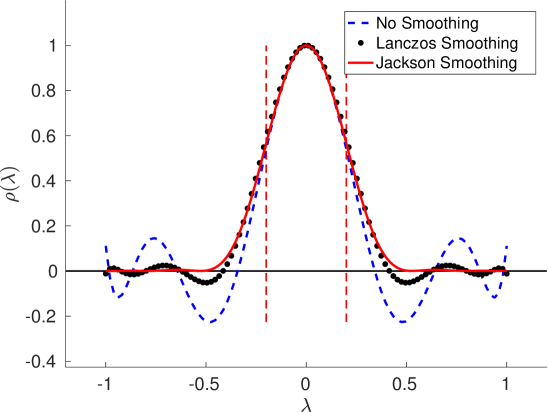
Figure 1: Polynomial filters $\rho_{k}$ of degree $k=11$ for the interval $[-0.2,0.2]$, using three different smoothing approaches.

2.4 Counting the eigenvalues in an interval

In order that the eigenvalues of $\bm{H}$ in $[\xi,\eta]$ can be computed numerically their number or at least a (tight) upper bound has to be known. After all, memory space has to be provided for storing the associated eigenvectors. Applying Sylvester’s law of inertia for counting the eigenvalues in an interval is infeasible because of the fill-in generated in the $\bm{LDL}^{T}$ factorization of $\bm{H}-\lambda\bm{I}$. However, we showed above that the number of the eigenvalues in an interval $[\xi,\eta]$ equals the trace of the spectral projector $\bm{P}_{[\xi,\eta]}=\chi_{[\xi,\eta]}(\bm{H})$ which we do not have available explicitly, but which we can approximate by a truncated Chebyshev series $\psi(\bm{H})$, i.e. $\psi(t)\approx\chi_{[\xi,\eta]}(t)$. Hutchinson [17] showed that ${\mathbb{E}}(\bm{v}^{*}\bm{Hv})=\operatorname*{trace}(\bm{H})$ holds for randomly generated vectors $\bm{v}$ with entries that are identically independently distributed (i.i.d.) random variables. Hutchinson originally used i.i.d. Rademacher random variables, where each entry of $\bm{v}$ assumes the value $-1$ or $1$ with probability $1/2$. In general, any sequence of random vectors $\bm{v}_{\ell}$ whose entries are i.i.d. random variables can be used, as long as the mean of their entries is zero [8]. Here, we use a Gaussian estimator to approximate $\operatorname*{trace}\bm{P}_{[\xi,\eta]}$,

$$\mu_{[\xi,\eta]}=\operatorname*{trace}\bm{P}_{[\xi,\eta]}\approx\mathcal{T}_{M}\equiv\frac{n}{M}\sum_{\ell=1}^{M}\bm{v}_{\ell}^{T}\psi_{k}(\bm{H})\bm{v}_{\ell},\qquad\lVert\bm{v}_{\ell}\rVert_{2}=1,$$ (19)

by using normally distributed variables for the entries of the random vectors $\bm{v}_{\ell}$. (The factor $n$ in (19) is due to the normalization of the $\bm{v}_{\ell}$.) Despite the fact that the Gaussian estimator has a larger variance than Hutchinson’s, it shows better convergence in terms of the number $M$ of sample vectors [4]. As in [18, 23, 26] we choose $\psi$ to be a truncated Chebyshev series for $\chi_{[\xi,\eta]}(t)$, such that

$$\gamma_{j}=\frac{\langle\chi_{[\xi,\eta]},T_{j}\rangle}{\langle T_{j},T_{j}\rangle},$$

according to (11)–(12). For the actual values of these integrals see (27) and (12).

2.5 Computing a basis of $\mathcal{R}(\texorpdfstring{\bm{P}}{p}_{[\xi,\eta]})$ with the thick-restart Lanczos algorithm

The desired eigenvectors $\bm{u}_{k}$ of $\bm{H}$ with eigenvalues $\lambda_{k}\in[\xi,\eta]$ span $\mathcal{R}(\bm{P}_{[\xi,\eta]})=\mathcal{R}(\chi_{[\xi,\eta]}(\bm{H}))$. In Algorithm 1 first a basis for $\mathcal{R}(\bm{P}_{[\xi,\eta]})$ is computed and then the eigenvectors are extracted from it by the Rayleigh–Ritz procedure [27]. Remember that if $\bm{u}_{k}\in\mathcal{R}(\bm{V})$ then $\lambda_{k}$ is an eigenvalue of $\bm{V}^{*}\!\bm{HV}$.

We consider two different procedures to generate a basis of $\mathcal{R}(\bm{P}_{[\xi,\eta]})$. The first is based on the thick-restart Lanczos algorithm [46] where the operator is the matrix polynomial $\rho_{k}(\bm{H})$. Our implementation follows closely the one described by Li et al. [21] that has been implemented in the EVSL library. The second procedure is based on subspace iteration with a polynomial filter designed precisely for this algorithm. It is presented in the next subsection.

The requirements for the polynomial filter are different for the Lanczos algorithm, for the subspace iteration, and for eigenvalue counting. In the latter the filter $\psi(t)\in{\mathbb{P}}_{d}$ has to be a good approximation of the characteristic function $\chi_{[\xi,\eta]}(t)$. As the Lanczos algorithm converges best towards extremal eigenvalues that are well separated from the rest of the spectrum [27], $\rho_{k}(t)$ must be (relatively) large in $[\xi,\eta]$ and small outside. Li et al. [21] suggest, as others before [45, 37, 38], to generate a filter that mimicks a Delta distribution, i.e., the functional $\delta(\cdot-\gamma)$ defined by

$$\int_{\infty}^{\infty}\delta(t-\gamma)\phi(t)\,dt=\phi(\gamma)$$

for all continuous functions $\phi$. In the set of polynomials of degree $k$, $\delta(t-\gamma)$ can be represented by

$$\rho_{k}(x)=\sum_{j=0}^{k}\frac{T_{j}(\gamma)}{\langle T_{j},T_{j}\rangle}T_{j}(x).$$ (20)

$\gamma\in(\xi,\eta)$ is chosen close to the interval midpoint such that $\tau:=\rho_{k}(\xi)=\rho_{k}(\eta)$. By construction, $\rho_{k}(x)>\tau$ in $(\xi,\eta)$. Eigenvectors of $\rho_{k}(\bm{H})$ corresponding to eigenvalues $>\tau$ are potential eigenvectors of $\bm{H}$. Care has to be taken, though, as different eigenvalues of $\bm{H}$ may be mapped to the same value by $\rho_{k}$. Nevertheless, the eigenvectors of $\rho_{k}(\bm{H})$ corresponding to eigenvalues $>\tau$ do span $\mathcal{R}(\bm{P}_{[\xi,\eta]})$. The correct eigenvalue-eigenvector relations can be found by a Rayleigh–Ritz procedure applied to $\bm{H}$. With this filter the eigenvalues close to $\xi$ and $\eta$ appear usually later than those inside $(\xi,\eta)$. Since $\mathcal{T}_{M}$ in (19) is only an approximation of $\mu_{[\xi,\eta]}$ we add some 10% to it to get a (heuristic) upper bound for the number of eigenvalues in $[\xi,\eta]$. Of course, a large overestimation of $\mu_{[\xi,\eta]}$ entails a waste of memory space.

2.6 Computing a basis of $\mathcal{R}(\texorpdfstring{\bm{P}}{p}_{[\xi,\eta]})$ with subspace iteration

In a second approach we compute a basis of $\mathcal{R}(\bm{P}_{[\xi,\eta]})$ with the subspace iteration. The polynomial filter $\pi_{k}\in{\mathbb{P}}_{k}$ is designed to satisfies (10) with $\tau=1$. $\varepsilon$ should be as small as possible such that $\lvert\pi_{k}(t)\rvert$ is smaller than some prescribed value outside $[\xi-\varepsilon,\eta+\varepsilon]$. To arrive at such a filter we first construct a piecewise polynomial $p$ that we then approximate by a Chebyshev series. We start with the derivative $q=p^{\prime}$ that we define by

$$q(x)=\begin{cases}0,&-1<x<\xi-\varepsilon,\\ \frac{2}{\varepsilon^{2}}(x-\xi+\varepsilon),&\xi-\varepsilon\leq x<\xi,\\ \frac{2}{\varepsilon(\xi-\eta)}(2x-\xi-\eta),&\xi\leq x<\eta,\\ \frac{2}{\varepsilon^{2}}(x-\eta-\varepsilon),&\eta\leq x<\eta+\varepsilon,\\ 0,&\xi-\varepsilon<x<1.\end{cases}$$ (21)

$q$ is a continuous piecewise linear polynomial. A plot of a typical $q$ is given on the left of Figure 2.

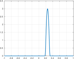
Figure 2: Plot of $q$ (left) and $p$ (right) for $\xi=0.2$, $\eta=0.3$ and $\varepsilon=0.025$. We have $q(\xi)=-q(\eta)=\frac{2}{\displaystyle\varepsilon}=80$ and $p(\frac{\xi+\eta}{2})=3$.

The anti-derivative $p$ of $q$ with $p(\xi)=p(\eta)=1$ is

$$p(x)=\begin{cases}0,&-1<x<\xi-\varepsilon,\\ \frac{1}{\varepsilon^{2}}(x-\xi+\varepsilon)^{2},&\xi-\varepsilon\leq x<\xi,\\ 1+\frac{1}{2\varepsilon(\eta-\xi)}((\eta-\xi)^{2}-(2x-\xi-\eta)^{2}),&\xi\leq x<\eta,\\ \frac{1}{\varepsilon^{2}}(x-\eta-\varepsilon)^{2},&\eta\leq x<\eta+\varepsilon,\\ 0,&\xi-\varepsilon<x<1.\end{cases}$$ (22)

We see that $p(x)>1$ in $(\xi,\eta)$ and that the maximal value that $p$ attains is at the center of $(\xi,\eta)$ where

$$p(\frac{\xi+\eta}{2})=1+\frac{\eta-\xi}{2\varepsilon}.$$

$p$ is symmetric with respect to $(\xi+\eta)/2$, i.e., $p((\xi+\eta)/2-x)=p((\xi+\eta)/2+x)$ whenever the values are defined. The piecewise quadratic $p$ is continuously differentiable by construction. Therefore, the convergence of the Chebyshev series is quick, the coefficients $\gamma_{j}$ in the series decay like $1/j^{3}$, see [42, Thm.7.1]. Also the Gibbs oszillations are not as prominent as with the approximation of a discontinuous function. If $(\xi,\eta)$ is at or close to the boundary of $(-1,1)$ we can define $p(x)$ as above. In the computation of the coefficients $\gamma_{j}$ in the Chebyshev series (13) only the piece of $p$ in $(-1,1)$ is to be taken onto account.

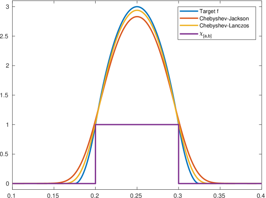
Figure 3: Plot of $p$ and Chebyshev-Jackson and Chebyshev-Lanczos polynomial expansions of degree $k=200$ for $\xi=0.2$, $\eta=0.3$ and $\varepsilon=0.025$. The violet curve shows the characteristic function $\chi_{[\xi,\eta]}$. The values of the Chebyshev-Jackson and Chebyshev-Lanczos polynomials at the critical points are, respectively, $\pi_{k}^{J}(\xi-\varepsilon)\approx 0.164$, $\pi_{k}^{J}(\eta+\varepsilon)\approx 0.154$, $\pi_{k}^{L}(\xi-\varepsilon)\approx 0.0624$, $\pi_{k}^{L}(\eta+\varepsilon)\approx 0.0578$.

The Chebyshev–Jackson (Chebyshev polynomial expansion with Jackson smoothing) $\pi_{k}^{J}(x)$, for $x=\xi-\varepsilon$ and $\eta+\varepsilon$, converges monotonically to zero ($=p(\xi-\varepsilon)=p(\eta+\varepsilon)$) from above. We can therefore determine the polynomial degree $k$ such that

$$\max\{\pi_{k}^{J}(\xi-\varepsilon),\pi_{k}^{J}(\eta+\varepsilon)\}\leq r\min\{\pi_{k}^{J}(\xi),\pi_{k}^{J}(\eta)\}.$$ (23)

A typical value for the convergence rate $r$ is $0.1$. We compare with the values of $\pi_{k}$ at $\xi$ and $\eta$ as they can be away from 1 for low degrees $k$. We check at both ends of the interval as the Chebyshev polynomials are not symmetric. If (23) is satisfied then the components in the directions of eigenvalues outside $(\xi-\varepsilon,\eta+\varepsilon)$ will decay with a rate below $r$ [27, 30]. So, the polynomial filter takes care of these directions, while the Rayleigh–Ritz procedure handles the directions associated with eigenvalues in $(\xi-\varepsilon,\xi)\cup(\eta,\eta+\varepsilon)$. For this to work, the search space in the subspace iteration must be at least as large as the number of eigenvalues in $(\xi-\varepsilon,\eta+\varepsilon)$.

By means of $\varepsilon$ and $r$ we can control the dimensions of subspaces and the number of iteration steps. The order of the filter polynomials increases if $\varepsilon$ and $r$ decrease. The order of the filter polynomial decreases if we switch from Jackson to Lanczos smoothing. If the subspace dimension gets to large we may split $(\xi,\eta)$ in smaller pieces. This so-called ‘spectrum slicing’ entails higher polynomial degrees [21].

3 Implementation

We combined the methods discussed in the previous section and a few other useful tools into a utility that can be employed to compute the eigenpairs of a $n\times n$ real symmetric (or complex Hermitian) matrix $\bm{H}$ within a specified interval of interest $[\xi,\eta]$ in parallel by simply providing an XML configuration file [2]. The outline of the utility is displayed in Algorithm 3.

 3. The BosonPeak Utility

1:  Import user-specified configuration via XML file.

2:  Import matrix $\bm{H}$.

3:  if requested then estimate extremal eigenvalues $\lambda_{\min},\lambda_{\max}$ of $\bm{H}$ using a few Lanczos steps.

4:  Transform the matrix $\bm{H}$ such that $-1\leq\lambda_{\min}<\lambda_{\max}\leq 1$, according to (5).

5:  if requested then estimate the number of eigenvalues in the specified interval $[\xi,\eta]$.

6:  Compute the polynomial filter $\rho_{k}$ or $\pi_{k}$.

7:  Compute the eigenpairs $({\lambda}_{j},\bm{u}_{j})$, $\lVert\bm{u}_{j}\rVert=1$, of $\bm{H}$ with ${\lambda}_{j}\in[\xi,\eta]$ and residual norms $r_{j}=\|\bm{H}\bm{u}_{j}-{\lambda}_{j}\bm{u}_{j}\|<\epsilon$ using either the thick restart Lanczos algorithm or subspace iteration.

8:  if requested then save eigenvalues ${\lambda}_{j}$, associated eigenvectors $\bm{u}_{j}$, and residual norms $r_{j}$ to disk.

The utility is written in C++11 and uses Trilinos [43] extensively. Trilinos is a collection of open-source software libraries, called packages, for the development of scientific applications.

The most basic Trilinos package is Epetra that provides classes for the construction and use of sequential and distributed parallel linear algebra objects. The Trilinos solver packages are designed to work with Epetra objects. The most used linear algebra objects in our implementation are (i) sparse matrices stored as Epetra_CrsMatrix objects in the compressed row storage (CRS) scheme, and (ii) Epetra_MultiVector objects that represent multivectors, i.e., collections of dense vectors. Each vector in an Epetra_MultiVector object is stored as a contiguous array of double-precision numbers. Both objects are extensively used for sparse matrix-vector multiplications in the various Trilinos solver packages. All Trilinos packages resort to a method called Epetra_Operator::Apply to multiply a matrix with a (multi)vector. Our operators are mostly matrix polynomials, and a call to Epetra_Operator::Apply entails the invocation of Algorithm 2.

Anasazi [5] is a package that offers a collection of algorithms for solving large-scale eigenvalue problems. As part of the package it provides solver managers to implement strategies for that purpose. We employ Anasazi’s block Krylov–Schur eigensolver with thick restarts. The subspace iteration that we discuss below is not a part of Anasazi. We implemented it ourselves, based on Epetra data structures.

The Teuchos package is a collection of common tools used throughout Trilinos. Among other things, it provides templated access to BLAS and LAPACK interfaces, parameter lists that allow to specify parameters for different packages, and memory management tools for aiding in correct allocation and deletion of memory.

Part of Teuchos’ memory management tools is an implementation of a smart Reference-Counted Pointer (RCP) class, which for an object tracks a count of the number of references to it held by other objects. Once the counter becomes zero, the object can be deleted. The advantage of a RCP is that the possibility of memory leaks in a program can be reduced. This is important when working with rather large objects, e.g., an Epetra_CrsMatrix object storing over $10^{9}$ nonzero entries. RCP objects are heavily used throughout our implementation to manage large objects, especially large temporary objects that are only needed during a fraction of the whole computation.

Trilinos supports distributed-memory parallel computations through the Message Passing Interface (MPI). Both the Epetra_CrsMatrix and the Epetra_Multivector objects can be used in a distributed memory environment by defining data distribution patterns using Epetra_Map objects.

The entries of a distributed object (such as rows or columns of an Epetra_CrsMatrix or the rows of an Epetra_Multivector) are represented by global indices uniquely over the entire object. A map essentially assigns global indices to available MPI ranks, which in our case corresponds to a single core of a processor.

For the addressing, local and global indices in Epetra use by default the $32$-bit int type. Since our implementation is based on the C++11 language standard and we want to allow computations with large matrices, we explicitly use $64$-bit global indices of type long long when working with distributed linear algebra objects. (Local indices are of type int.)

An Epetra_Map object encapsulates the details of distributing data over MPI ranks. In our implementation, we use contiguous and one-to-one maps for the block row-wise distribution of the Epetra_CrsMatrix and Epetra_MultiVector objects. Contiguous means that the list of global indices on each MPI rank forms an interval and is strictly increasing. A one-to-one map allows a global index to be owned by a single rank. For the columns, the distribution pattern we are using distributes the complete set of global column indices for a given global row, meaning that if a rank $p$ owns the global row index $i$, it also owns all global column indices $j$ on that row, thus having local access to the global entry $(i,j)$. The map used for the distribution of the columns is thus not a one-to-one map, since a global column index can be owned by multiple ranks.

The matrix import implemented in the utility allows to efficiently import large matrices stored in a HDF5 file directly to an Epetra_CrsMatrix object. HDF5 is a data model, library, and file format for storing and managing data collections of all sizes and complexity. One of the advantages of using the HDF5 file format to store and import large matrices is the possibility to use MPI to read the HDF5 files in parallel. For this reason Trilinos provides the EpetraExt::HDF5 class for importing a matrix stored in a HDF5 file to a Epetra_CrsMatrix.

Since the EpetraExt::HDF5 class currently does not provide an import function for matrices with $64$-bit global indices of type long long, we extended the class by this functionality. The BosonPeak utility also provides a Python script that can be used to convert matrices stored in the MatrixMarket format to a HDF5 file suitable for import. The utility is described in detail in [2].

We now discuss two ways of computing the eigenvectors associated with the eigenvalues of a prescribed interval $[\xi,\eta]$. The first is an implementation of the thick-restart Lanczos algorithm applied to $\rho_{k}(\bm{H})$. We follow closely the implementation in EVSL, see [21]. $\rho_{k}(t)$ is an approximation of the Dirac delta distribution $\delta(t-\gamma)$ in ${\mathbb{P}}_{k}$ as given in (20). $\gamma\approx(\xi+\eta)/2$ is chosen such that $\rho_{k}(\xi)=\rho_{k}(\eta)=\tau$. The smaller $\tau$ (relative to $\rho_{k}(\gamma)$) the more prominent are the eigenvalues $\rho_{k}(\lambda_{j})$ for $\lambda_{j}\in[\xi,\eta]$ compared with the eigenvalues outside of this interval. Thus, the Lanczos algorithm will extract these eigenvalues quickly. The Lanczos algorithm also rapidly finds eigenvalues at the other end of the spectrum, $\rho_{k}(\lambda_{j})\approx 0$. But those are easily identified and discarded. Eigenpairs $(\mu_{j},\bm{v}_{j})$ of $\rho_{k}(\bm{H})$ with $\mu_{j}\geq\gamma$ are related to some eigenpair $(\lambda_{j^{\prime}},\bm{u}_{j^{\prime}})$ of $\bm{H}$. Certainly $\mu_{j}=\rho_{k}(\lambda_{j^{\prime}})$. Unless $\mu_{j}$ is simple, $\bm{v}_{j}$ may not be an eigenvector of $\bm{H}$. The reason for this is that it can happen that $\mu_{j}=\rho_{k}(\lambda_{j^{\prime}})=\rho_{k}(\lambda_{j^{\prime\prime}})$, $\lambda_{j^{\prime}}\neq\lambda_{j^{\prime\prime}}$, in which case $\bm{v}_{j}$ may be a linear combination of the eigenvectors $\bm{u}_{j^{\prime}}$ and $\bm{u}_{j^{\prime\prime}}$, and possibly others. The best way out of this problem is to execute a Rayleigh–Ritz procedure [27] that involves all eigenvectors $\bm{v}_{j}$ of $\rho_{k}(\bm{H})$ associated with eigenvalues $\geq\tau$. We employ the Lanczos algorithm with blocks of size 16, 32, or 64. The dimension of the search space is limited by $3n_{\text{ev}}$, where $n_{\text{ev}}$ is the number of desired eigenvalues. We consider eigenpairs converged if $\lVert\rho_{k}(\bm{H})\bm{u}_{i}-\rho_{k}(\lambda_{i})\bm{u}_{i}\rVert<\epsilon\lVert\rho_{k}(\bm{H})\rVert\lVert\bm{u}_{i}\rVert\leq\epsilon\rho_{k}(\gamma)\lVert\bm{u}_{i}\rVert$ with $\epsilon=10^{-6}$. This does not imply that $\lVert\bm{H}\bm{u}_{i}-\lambda_{i}\bm{u}_{i}\rVert<\epsilon\lVert\bm{H}\rVert\lVert\bm{u}_{i}\rVert$, though.

The second approach to compute the eigenvectors associated with eigenvalues in $[\xi,\eta]$ is based on a subspace iteration with the matrix $\pi_{k}(\bm{H})$. Note that in Algorithm 4 $\bm{H}$ should be substituted by $\pi_{k}(\bm{H})$.

 4. Subspace Iteration complemented by the Rayleigh–Ritz procedure

0:  Symmetric positive definite matrix $\bm{H}\in{\mathbb{R}}^{n\times n}$; number $p$ of desired eigenpairs; initial subspace $\bm{X}_{0}\in{\mathbb{R}}^{n\times q}$ with $q\geq p$; tolerance $\tau$.

0:  $n\times p$ matrix $\bm{X}$ and $\bm{\Lambda}=\operatorname*{diag}\{\lambda_{1},\ldots,\lambda_{p}\}$ with $\lambda_{1}\geq\cdots\geq\lambda_{p}$ such that

$$\lVert\bm{H}\bm{x}_{i}-\lambda_{i}\bm{x}_{i}\rVert<\tau,\qquad 1\leq i\leq p.$$

1:  Orthonormalize starting vectors $\bm{X}_{0}$./* Gram–Schmidt orthogonalization by QR factorization */

2:  for $k=1,\ldots$ do

3:     if $k\equiv 1\ (\text{mod}\ n_{\text{RR}})\ \&\ k>1$ then

4:        $\bm{Y}_{k}=\bm{HX}_{k-1}$;

5:        $\bm{R}=\bm{Y}_{k}-\bm{X}_{k-1}\bm{\Lambda}_{k-1}$;/* Residual $\bm{R}=[\bm{r}_{1},\ldots,\bm{r}_{q}]$ */

6:        $n_{\text{conv}}=\lvert\{1\leq i\leq q\ |\ \lVert\bm{r}_{i}\rVert<\tau\}\rvert$ /* Number of converged eigenpairs */

7:        if $n_{\text{conv}}\geq p$ then return ($\bm{X}=\bm{X}_{k}$, $\bm{\Lambda}=\bm{\Lambda}_{k}$); end if

8:        $\bm{X}_{k}=\bm{Y}_{k}$;

9:     else if $k\equiv-1\ (\text{mod}\ n_{\text{RR}})$ then

10:        $\bm{X}_{k}\bm{R}_{k}=\bm{HX}_{k-1}$; /* Iteration step with basis orthogonalization (QR) */

11:     else if $k\equiv 0\ (\text{mod}\ n_{\text{RR}})$ then

12:        $\bm{Y}_{k}=\bm{HX}_{k-1}$;

13:        $\bm{X}_{k}\bm{R}_{k}=\bm{Y}_{k}$;/* Orthonormalize $\bm{Y}_{k}$ (QR factorization) */

14:        $\bm{U}_{k}\bm{\Lambda}_{k}\bm{V}_{k}^{*}=\bm{R}_{k}$;/* Singular value decomposition */

15:        $\bm{X}_{k}=\bm{X}_{k}\bm{U}_{k}$; /* Ritz vectors */

16:     else

17:        $\bm{X}_{k}=\bm{HX}_{k-1}$; /* Simple iteration step */

18:     end if

19:  end for

The degree $k$ of $\pi_{k}$ should be the smallest integer for which condition (23) is satisfied. If $r=0.1$ and the search subspace is not smaller than $q=\mu_{[\xi-\varepsilon,\eta+\varepsilon]}$, the number of eigenvalues of $\bm{H}$ in $[\xi-\varepsilon,\eta+\varepsilon]$, then convergence is rapid: the angle between Ritz vectors and corresponding eigenvectors decreases per iteration step by the factor $r$. Also the residual norm, which defines our stopping criterion, decreases rapidly. One could try to determine the number of iteration steps in advance, based on $r$ and $\varepsilon$. Note that $r$ can be arbitrarily close to 1 if $\varepsilon\approx 0$. The larger $\varepsilon$, the smaller $k$ and the bigger $\mu_{[\xi-\varepsilon,\eta+\varepsilon]}$. The former is proportional to work; the latter determines the size of the search space. In subspace iteration the memory space for two multivectors of size $n\times\mu_{[\xi-\varepsilon,\eta+\varepsilon]}$ are needed. More memory is required in Algorithm 2. The actual amount depends on the block size.

Algorithm 4 follows quite closely the one proposed by Rutishauser [29], see also [27, Table 14.4]. The positive integer $n_{\text{RR}}$ indicates the frequency with which the Rayleigh–Ritz procedure is applied. In the iteration step before the RR procedure, the basis vectors in $\bm{X}_{k}$ are orthonormalized. In the iteration step after the RR procedure, the convergence criterion is applied. In our experiments we set $n_{\text{RR}}=6$ which, combined with $\tau=10^{-6}$, means that we have convergence after $n_{\text{RR}}$ iteration steps.

Considerable savings can be achieved by locking converged Ritz vectors. If $n_{\text{conv}}<p$ vectors have converged then only the columns $n_{\text{conv}}\!+\!1,\ldots,q$ have to be iterated. So, in lines 10, 12, and 17, a reduced number of columns have to be multiplied by $\bm{H}$. In order to profit from locking we increase $r$, setting $r=\sqrt{.1}$ or $r=\sqrt[4]{.1}$. This means that we have convergence only after $2n_{\text{RR}}$ or $4n_{\text{RR}}$ iteration steps. However, the degree of the polynomial smoother is reduced considerably such that, combined with locking, shorter execution times can result.

4 Numerical experiments

4.1 Comparisons by means of synthetic problems

To compare solvers and filters we first limit ourselves to synthetic diagonal eigenvalue problems. We construct diagonal matrices $\bm{H}$ that have a prescribed eigenvalue distribution. The eigenvalues in intervals $(\xi,\eta)$ are then computed by either subspace iteration or thick-restart Lanczos, both with polynomial filtering. We know in advance how many eigenvalues we are looking for, whence we do not estimate this number. The filter maps these $p$ eigenvalues to the largest of the filtered matrix. In subspace iteration (SI) we iterate with a block size $q$ which is initially the number of eigenvalues of $\bm{H}$ in $(\xi-\varepsilon,\eta+\varepsilon)$. $q$ decreases as the number of found eigenpairs increases. In the block Lanczos algorithm the block size is fixed to 8. The block Lanczos algorithm with thick restart (TRLanczos) is implemented in Anasazi as a variant of the block Krylov–Schur (BKS) algorithm [5]. Note that we use the notions TRLanczos and BKS interchangeably.

We measure the computational effort by matrix-vector multiplications (MatVec’s). In realistic computations the MatVec’s dominate Rayleigh–Ritz procedure or thick restart. In both SI and BKS the computational effort is the number of iteration steps times the degree of the polynomial filter times the block size.

	SI + Piecewise quadratic polynomial filter
	Jackson smoothing		Lanczos damping		No smoothing
	$d$	#MatVec’s	$d$	#MatVec’s	$d$	#MatVec’s
$r=0.1$	5’753	3’020’325	3’508	1’841’700	1’163	1’099’035
$r=\sqrt{0.1}$	2’739	2’670’525	1’771	1’726’725	893	870’675
$r=\sqrt[4]{0.1}$	1’548	2’616’120	1’058	1’788’020	673	1’137’370
	SI + Dirac polynomial filter
	Jackson smoothing		Lanczos damping		No smoothing
	$d$	#MatVec’s	$d$	#MatVec’s	$d$	#MatVec’s
$\phi=0.8$	942	3’706’770	696	2’724’840	494	1’822’860
$\phi=0.6$	1’412	2’760’460	1’034	1’747’460	727	1’206’820
	BKS + Piecewise quadratic polynomial filter
	Jackson smoothing		Lanczos damping		No smoothing
	$d$	#MatVec’s	$d$	#MatVec’s	$d$	#MatVec’s
$r=0.1$	5’753	828’432	3’508	505’152	1’163	167’472
$r=\sqrt{0.1}$	2’739	394’416	1’771	255’024	893	207’176
$r=\sqrt[4]{0.1}$	1’548	359’136	1’058	245’456	673	156’136
	BKS + Dirac polynomial filter
	Jackson smoothing		Lanczos damping		No smoothing
	$d$	#MatVec’s	$d$	#MatVec’s	$d$	#MatVec’s
$\phi=0.8$	942	301’440	696	222’720	494	201’552
$\phi=0.6$	1’412	327’584	1’034	239’888	727	168’664

Table 1: Summary of test runs with subspace iteration and various polynomial filters. Equally distributed eigenvalues. $\xi=-0.9$, $\eta=-0.898$, $\varepsilon=0.0005$, $p=50$, $q=75$ in SI, BKS block size is 8. Best performance is in bold.

We consider three test cases, all with diagonal matrices of order 50’000. In the first case the matrix $\bm{A}$ has equally distributed eigenvalues in $[-1,1]$. We computed the 50 eigenvalues in the interval $(\xi,\eta)=(-0.9,-0.898)$. In this test case as in later ones we start the iterations with (the same) random multivector of the appropriate size. The progress of the algorithm depends of course on the initial data. However, the results given here represent typical behavior. We did not execute an exhaustive search for best parameters, though. The results for the first test matrix with equidistant eigenvalues are presented in Table 1. The block Krylov–Schur algorithm clearly outperforms subspace iteration, by a factor 5 when comparing the best parameter sets. There is no clear winner among the polynomial filters. Both types of filters perform best without smoothing. The reduction of the polynomial degree is larger than the gain by smoothing or damping the Gibbs oscillations. This holds particularly for the piecewise quadratic polynomial filter. The Dirac polynomial filter performs better with $\phi=0.6$ than with $\phi=0.8$, i.e., with the better approximation of the Dirac distribution. This leads to higher polynomial degrees, but to lower iteration counts. On the other hand, the piecewise quadratic polynomial filter prefers a weak approximation of the step function, $r>0.1$, but the results are not consistent. With SI this increases the iteration count but decreases the cost of a single iteration step and increases the potential for locking.

	SI + Piecewise quadratic polynomial filter
	Jackson smoothing		Lanczos damping		No smoothing
	$d$	#MatVec’s	$d$	#MatVec’s	$d$	#MatVec’s
$r=0.1$	5’764	645’568	3’498	391’776	1’220	223’260
$r=\sqrt{0.1}$	2’663	527’274	1’702	336’996	662	134’386
$r=\sqrt[4]{0.1}$	1’389	486’150	904	316’400	485	169’750
	SI + Dirac polynomial filter
	Jackson smoothing		Lanczos damping		No smoothing
	$d$	#MatVec’s	$d$	#MatVec’s	$d$	#MatVec’s
$\phi=0.8$	472	722’160	349	512’681	249	360’801
$\phi=0.6$	708	477’192	519	347’211	365	221’920
	BKS + Piecewise quadratic polynomial filter
	Jackson smoothing		Lanczos damping		No smoothing
	$d$	#MatVec’s	$d$	#MatVec’s	$d$	#MatVec’s
$r=0.1$	5’764	276’672	3’498	167’904	1’220	107’360
$r=\sqrt{0.1}$	2’663	149’128	1’702	95’312	662	74’144
$r=\sqrt[4]{0.1}$	1’389	88’896	904	65’088	485	62’080
	BKS + Dirac polynomial filter
	Jackson smoothing		Lanczos damping		No smoothing
	$d$	#MatVec’s	$d$	#MatVec’s	$d$	#MatVec’s
$\phi=0.8$	472	30’208	349	41’880	249	47’808
$\phi=0.6$	708	45’312	519	53’976	365	70’080

Table 2: Summary of test runs with subspace iteration and various polynomial filters. Eigenvalue density increasing towards $+1$. $\xi=-0.9$, $\eta=-0.896$, $\varepsilon=0.0005$, $p=10$, $q=16$ in SI, BKS block size is 8. Best performance is in bold.

The density of the eigenvalues of the matrix $\bm{H}$ of the second test case increases from $-1$ to 1. In the interval that we chose, $(\xi,\eta)=(-0.9,-0.896)$, there are only 10 eigenvalues. These are better separated from the rest of the spectrum than in the previous test case. The interval in this example is twice as wide as in the previous example. Therefore, the polynomial degrees are lower. Note that the filter polynomials only depend on the interval, not on the number of eigenvalues it contains.

The results of the second test are given in Table 2. Here, the thick restart Lanczos (BKS) algorithm with the Dirac filter ($\phi=0.8$) and Jackson smoothing is twice as fast as BKS with the piecewise quadratic polynomial filter ($r=\sqrt[4]{0.1}$) without smoothing and more than four times faster than any combination of subspace iteration.

	SI + Piecewise quadratic polynomial filter
	Jackson smoothing		Lanczos damping		No smoothing
	$d$	#MatVec’s	$d$	#MatVec’s	$d$	#MatVec’s
$r=0.1$	1’521	958’230	924	582’120	328	290’280
$r=\sqrt{0.1}$	709	825’985	454	528’910	180	209’700
$r=\sqrt[4]{0.1}$	373	630’370	244	412’360	130	230’480
	SI + Dirac polynomial filter
	Jackson smoothing		Lanczos damping		No smoothing
	$d$	#MatVec’s	$d$	#MatVec’s	$d$	#MatVec’s
$\phi=0.8$	128	945’280	95	679’725	68	458’660
$\phi=0.6$	192	668’745	141	487’155	100	321’000
	BKS + Piecewise quadratic polynomial filter
	Jackson smoothing		Lanczos damping		No smoothing
	$d$	#MatVec’s	$d$	#MatVec’s	$d$	#MatVec’s
$r=0.1$	1’521	292’032	924	177’408	328	102’336
$r=\sqrt{0.1}$	709	136’128	454	250’608	180	56’160
$r=\sqrt[4]{0.1}$	373	71’616	244	46’848	130	56’160
	BKS + Dirac polynomial filter
	Jackson smoothing		Lanczos damping		No smoothing
	$d$	#MatVec’s	$d$	#MatVec’s	$d$	#MatVec’s
$\phi=0.8$	128	39’936	95	29’640	68	29’376
$\phi=0.6$	192	59’904	141	43’992	100	67’200

Table 3: Summary of test runs with subspace iteration and various polynomial filters. Eigenvalue density increasing towards $+1$. $\xi=-0.9$, $b=-0.885$, $\varepsilon=0.002$, $p=66$, $q=90$, BKS block size 8. Best performance is in bold.

In the third test case we chose the same matrix as in the second but we expanded the search interval to have about the same number of eigenvalues as in the first test case. The interval $(\xi,\eta)=(-0.9,-0.885)$ encloses 66 eigenvalues that form a superset of the eigenvalues of the matrix in test case 2. While the eigenvalue count is more than 6 times higher, the degrees of the filter polynomials decreases by a factor of almost 4. This has the effect that the costs with respect to test example 2 increase slightly for SI and even decrease for BKS, see Table 3. The outcome is similar to case 2. BKS with Dirac polynomial filtering ($\phi=0.8$) is faster than BKS with piecewise quadratic polynomial filtering by a factor almost two and faster than any varian of SI by a factor almost 7. In contrast to test case 2, here no smoothing or Lanczos damping perform better than Jackson smoothing.

Based on these results we decided to employ the Trilinos block Krylov–Schur eigensolver combined with the Dirac polynomial filter with $\phi=0.8$ in the real world problems treated below. We chose to employ Jackson smoothing as our real world problems most resemble test case 2: we compute a few eigenvalues w.r.t. the problem size and the eigenvalue density increases towards higher eigenvalues.

4.2 A realistic application: a glassy structure

For a preliminary usage of the developed algorithm, we explore the spectrum of a set of instances of a glassy structure involving $N=256^{\prime}000$ atoms. The atomic positions of this structure are produced through a series of molecular dynamics simulations involving: a well-equilibrated liquid at temperatures well above the melting temperature, a quench to the lower temperatures of the amorphous solid regime, and a final relaxation which brings the system to a local potential energy minimum from which the dynamical matrices of order $3\!\times\!256^{\prime}000=768^{\prime}000$ can be calculated. Note that different equivalent initial distribution of the atoms lead to different realizations of the configuration. The empirical atomic interaction model used to perform these simulations is based on a Lennard–Jones force model [44], which describes the interaction between atoms of two types differing in both size and mass. Periodic boundary conditions are used to remove the explicit structural effect of a surface. For the chosen density, the periodicity length is $L=101.714585$ where the unit distance is close to the average atomic bond length. Details of the sample preparation procedure and the resulting glassy structures may be found in refs. [11, 13, 12]. These aspects entail a set of sparse dynamical matrices, $\bm{H}_{i}$, which have $\sim\!250$ nonzero elements per row, cf. column 2 in Table 4. The sparsity of the matrices is thus about $3\cdot 10^{-4}$. Each of these matrices represents one realisation of a configuration.

Past work considering much smaller glassy atomic configurations using the Lennard–Jones potential [14] suggests that the eigenvalue regime at which sound breaks up – the so-called boson peak (PB) regime – occurs in the approximate $\lambda$-interval $[1,2]$, where $\lambda_{\max}$ was around 1800. Since the infinite-dimensional operator underlying (3) is bounded, we do not expect $\lambda_{\max}$ to increase much with increased system size. Indeed, the matrices $\bm{H}_{i}$ all have their eigenvalues in the interval $[0,1920]$. We are looking for those in the two subintervals $[\xi,\eta]=[0.1,1]$ and $[\xi,\eta]=[1,2]$ that are mapped by the linear function (5) to $[-\frac{9599}{9600},-\frac{9590}{9600}]\approx[-0.99990,-0.99896]$ and $[-\frac{9590}{9600},-\frac{9580}{9600}]\approx[-0.99896,-0.99792]$, respectively. These computations were part of an exploration of the eigenstructure of the $\bm{H}_{i}$ down to a value of $\lambda=0$.

		$(\xi,\eta)=(0.1,1)$			time	$(\xi,\eta)=(1,2)$			time
		$\text{degree}(\rho_{k})=121$			to	$\text{degree}(\rho_{k})=156$			to
Matrix	nnz($\bm{H}_{i}$)	# EVs			sol’n	# EVs			sol’n
		true	est.	req	[sec]	true	est.	req	[sec]
$\bm{H}_{1}$	$191^{\prime}893^{\prime}806$	249	259	300	$1^{\prime}225$	819	798	900	$4^{\prime}059$
$\bm{H}_{2}$	$191^{\prime}883^{\prime}888$	236	233	300	$1^{\prime}224$	794	780	900	$3^{\prime}637$
$\bm{H}_{3}$	$191^{\prime}903^{\prime}166$	239	249	300	$1^{\prime}243$	811	793	900	$4^{\prime}551$
$\bm{H}_{4}$	$191^{\prime}851^{\prime}848$	249	262	300	$1^{\prime}242$	826	812	900	$4^{\prime}600$
$\bm{H}_{5}$	$191^{\prime}832^{\prime}588$	249	259	300	$1^{\prime}196$	828	807	900	$4^{\prime}094$
$\bm{H}_{6}$	$191^{\prime}859^{\prime}012$	259	262	300	$1^{\prime}218$	820	817	900	$4^{\prime}169$
$\bm{H}_{7}$	$191^{\prime}887^{\prime}542$	238	248	300	$1^{\prime}220$	820	796	900	$4^{\prime}159$
$\bm{H}_{8}$	$191^{\prime}853^{\prime}378$	245	259	300	$1^{\prime}206$	806	806	900	$4^{\prime}146$

Table 4: Results for the partial eigenvalue computations of the Hessians $\bm{H}_{1},\ldots,\bm{H}_{8}$ with $N=256^{\prime}000$ atoms, i.e., order $n=768^{\prime}000$. $\text{nnz}(\bm{H}_{i})$ denotes the number of nonzeros of $\bm{H}_{i}$. The time to solution shows the time of the eigensolver part of the utility (line 7 in Algorithm 3). It is with respect to the computations with 48 cores on Euler II.

A survey of results for the partial eigenvalue computations of the Hessians $\bm{H}_{1},\ldots,\bm{H}_{8}$ is given in Table 4. For each matrix $\bm{H}_{i}$ and each interval $[\xi,\eta]$ we give the true and estimated numbers of eigenvalues in the respective interval and the time to compute the former. The true numbers of eigenvalues are obtained as a result of the computations that targeted at 300 eigenvalues for the left interval and 900 for the right interval. These are $10-20\%$ more eigenvalues than estimated and, as such, a crude upper bound for $\mu_{[\xi,\eta]}$. The estimates have been obtained by the technique discussed in subsection 2.4 with $M=30$ samples in (19) and degree $k=100$ for which parameters de Napoli et al. [26] report very good results. One has to be careful when choosing $k$, though. $\psi_{k}$ has to be a reasonably good approximation of $\chi_{[\xi,\eta]}$. Otherwise the estimation may be completely off. Generally, $k$ should increase as the width of $[\xi,\eta]$ shrinks.

We computed the eigenvalues of the $\bm{H}_{i}$ with Anasazi’s block Krylov–Schur (BKS) algorithm (in fact, the thick restarted block Lanczos algorithm) with the same parameter values. The block size was fixed at 4. The number of blocks was limited to 225. The maximal dimension of the Krylov space was set to $3\times n_{\text{ev}}$, where $n_{\text{ev}}$ is the number of desired eigenvalues. The number of blocks was thus limited to $\frac{3\times n_{\text{ev}}}{\text{block size}}$. The threshold was set to $\tau=0.9$.

We have implemented the operator $\rho_{k}(\bm{H}_{i})$ in Trilinos. The degree $k$ of the filter polynomial is given in Table 4. One call of the operator amounts to the execution of $k$ matrix-multivector multiplications. Remember that the block size is 4. These $4k$ MatVec’s constitute more than 99% of the execution time of the solver.

The computations were carried out on Euler II of ETH Zurich’s compute cluster. Euler II comprises 768 compute, each equipped with two 12-core Intel Xeon E5-2680v3 processors (2.5-3.3 GHz) and between 64 and 512 GB of DDR4 memory. Euler II also contains 4 very large memory nodes each equipped with four 16-core Intel Xeon E7-8867v3 processors (2.5 GHz) and 3072 GB of DDR4 memory.

In the specified environment, our implementation worked with OpenMPI 1.65, HDF5 1.8.12, Boost 1.57.0, and Trilinos 12.2.1. Further, the code has been compiled with GCC 4.8.2 and the following optimization flags:

-ftree-vectorize -march=corei7-avx -mavx -std=c++11 -O3.

The convergence criterion requires that the residual norms

$$\lVert\rho_{k}(\bm{H}_{i})\bm{u}_{j}-\mu_{j}\bm{u}_{j}\rVert<\epsilon,\qquad\epsilon=10^{-6},\quad\lVert\bm{u}_{j}\rVert=1,$$

for all requested eigenpairs $(\mu_{j},\bm{u}_{j})$. This lead to very accurate eigenpairs of the original matrices,

$${r}_{j}\equiv\lVert\bm{H}_{i}\bm{u}_{j}-\lambda_{j}\bm{u}_{j}\rVert<3.5\cdot 10^{-8},\quad\lVert\bm{u}_{j}\rVert=1,$$

or better for all desired (true) eigenpairs $(\lambda_{j},\bm{u}_{j})$. Since we compute too many eigenpairs, the desired ones are finally too accurate. So, it is important for good efficiency to have accurate estimates for the eigenvalue counts. A high security margin entails high computational and memory costs, together with overly accurate results. The times to find the 300 largest eigenvalues and associated eigenvectors of $\rho_{k}(\bm{H}_{i})$ in the interval $[0.1,1]$ are in the average $1^{\prime}222$ sec with small variance. The 900 eigenpairs in the interval $[1,2]$ take about $4^{\prime}177$ sec to compute with larger variance. We attribute the large variance to the heterogeneous cluster and the larger execution times.

4.3 Scalability study

To test the parallel scalability of our code we consider a much larger glassy structure comprising of $1^{\prime}372^{\prime}000$ atoms. The Hessian matrix has now order $n=4^{\prime}116^{\prime}000$ and $1^{\prime}028^{\prime}329^{\prime}164$ nonzero entries. The number of nonzeros per row is again about 250, leading to a sparsity of $6\cdot 10^{-5}$.

In Table 5 we display the computational results for five subintervals of the investigated interval $[1,2]\subset[0,\lambda_{\max}(\bm{H})]$ with $\lambda_{\max}(\bm{H})=1941$. These computations were carried out on Euler V, the newest extension of ETH Zurich’s compute cluster. Euler V contains 352 compute nodes (Hewlett-Packard BL460c Gen10), each equipped with two 12-core Intel Xeon Gold 5118 processors (2.3 GHz nominal, 3.2 GHz peak) and 96 GB of DDR4 memory clocked at 2400 MHz. We consider Euler V a homogeneous cluster.

blk	#	dim	re-	# blk	poly	#	$\xi$	$\eta$	evs	evs	evs	time
size	blks	$\mathcal{K}_{d}$	starts	steps	degree	MatVec’s			est	req	true	[sec]
8	21	168	3	63	$10^{\prime}142$	$5^{\prime}111^{\prime}568$	1.169	1.183	49	55	46	$22^{\prime}667$
8	21	168	3	77	$10^{\prime}202$	$6^{\prime}284^{\prime}432$	1.183	1.197	49	55	48	$27^{\prime}959$
8	21	168	4	91	$10^{\prime}262$	$7^{\prime}470^{\prime}736$	1.197	1.211	50	55	54	$32^{\prime}937$
8	48	384	2	80	$5^{\prime}175$	$3^{\prime}312^{\prime}000$	1.211	1.239	101	128	106	$14^{\prime}647$
8	48	384	2	80	$5^{\prime}233$	$3^{\prime}349^{\prime}120$	1.239	1.267	103	128	105	$14^{\prime}850$

Table 5: Computational results for large glassy structure. $\xi$, $\eta$ are given with reference to the interval $[0,1941]$. The number of matrix-vector multiplications (#MatVec) equals (blk size)$\times$(#blk steps)$\times$(poly degree). Times are for 360 cores on Euler V.

evs	evs	deg	$p=360$		$p=720$		‘speedup’
conf	found		#blk steps	time	#blk steps	time
55	46	$10^{\prime}142$	63	$22^{\prime}667$	63	$11^{\prime}570$	1.96
55	48	$10^{\prime}202$	77	$27^{\prime}959$	63	$11^{\prime}506$	2.43
55	54	$10^{\prime}262$	91	$32^{\prime}937$	77	$14^{\prime}229$	2.31
128	106	$5^{\prime}175$	80	$14^{\prime}647$	112	$10^{\prime}570$	1.39
128	105	$5^{\prime}233$	80	$14^{\prime}850$	112	$10^{\prime}547$	1.41

Table 6: Execution times for $p=360$ and $p=720$ cores for the intervals in Table 5 and derived speedups.

There are three intervals of length 0.014 with about 50 eigenvalues and two intervals of length 0.028 with about 105 eigenvalues. We chose equal block size 8 for all computations. The number of blocks was again limited to $\frac{3\times n_{\text{ev}}}{\text{block size}}$ with $n_{\text{ev}}$ the number of requested eigenvalues. The maximal dimension of the Krylov space equals the block size times the number of blocks. If it is attained then a restart is issued. The number of restarts is obtained by the number of block steps divided by the number of blocks.

Interestingly, it is faster to compute the 105 eigenvalues in the longer intervals than the 50 eigenvalues in the shorter ones, essentially because of the lower degrees of the filter polynomials. Also the maximal dimension of the search space is relatively larger. This eases the extraction of the desired information. The overhead due to reorthogonalizations is negligible. The times in Table 5 are very well in proportion with the number of MatVec’s. We consistently observe 226 MatVec’s per sec. The times given are the fastest out of three runs.

In Table 6 we replicate the execution times of Table 5 for 360 cores and complement them with the execution times obtained with 720 cores. 360 cores correspond to 15 nodes; 720 cores correspond to 30 nodes of Euler V. Evidently, the runs with 720 cores should take only half the time of the ones on 360 cores, amounting to a speedup of two. Since most of the computing time is spent in (blocked) matrix-vector multiplications a speedup close to two can indeed be expected. The data is distributed among the cores in the standard block row-wise fashion of Trilinos. The computations are similar, in particular, the initial vectors are equal. Nevertheless, the number of iteration steps until convergence can differ significantly. Therefore, the speedup appears to be erratic. However, if we compare the execution times of the single block steps, then we observe speedups close to two, more precesely between 1.94 and 1.988. With 720 cores about 443 MatVec’s are executed per second.

4.4 Physics results

In what follows, the eigenmode $\bm{q}$ is seen as consisting of $N$ 3-vectors, $\bm{q}_{i}=(q_{i}^{1},q_{i}^{2},q_{i}^{3})$, where the superscript indicates the coordinate direction. To gain an estimate of the number of atoms involved in a normalized eigenmode the participation ratio [9] is used,

$$\mathrm{PR}=\frac{1}{\sum_{i}|\bm{q}_{i}|^{4}}=\frac{1}{\lVert\bm{q}\rVert_{4}^{4}},$$ (24)

where $\lVert\bm{q}\rVert_{2}=1$ is assumed. When an eigenmode has constant values, say $|\bm{q}_{i}|=1/\sqrt{N}$ then $\mathrm{PR}=1$ and all atoms are said to partake in the eigenmode. On the other hand when $\lvert\bm{q}_{i}\rvert=1$ for the $i$th atom and $\lvert\bm{q}_{j}\rvert=0$ for all other atoms $j\neq i$, then $\mathrm{PR}=1/N$. For a plane (sound) wave of wave-vector $\bm{k}$ we have $\bm{q}_{i}=\sqrt{2/N}\,\hat{\bm{\zeta}}_{\bm{q}}\sin\bm{k}\cdot\bm{q}_{i}$ entailing a $\mathrm{PR}=2/3$. Here $\hat{\bm{\zeta}}_{\bm{q}}$ is termed the polarization vector and is usually taken as being perpendicular (transverse sound) or parallel (longitudinal sound) to $\bm{k}$.

Fig. 4 plots the participation ratio of the entire spectrum considered in the present work. At $\lambda=0$, there exist three modes with a participation ratio equal to unity, which correspond to the translational modes of the dynamical matrix. For the region up to approximately, $\lambda=0.5$, the eigenvalues are seen to bunch into clusters with a participation ratio of approximately 2/3, indicating plane-wave-like eigenmodes and the presence of well defined sound. The observed bunching and their multiplicity arise from a combination of the polarization vectors, $\hat{\bm{\zeta}_{\bm{k}}}$, and the allowed wave-vectors, $\bm{k}_{[mnl]}=2\pi/L(m,n,l)$. Here $L$ is the periodicity length of the amorphous configuration, and $m$, $n$, and $l$ are integers defining the allowed wave-lengths. Through inspection of the corresponding eigenmodes, a wave-vector family and polarization type can be identified for each bunching and are indicated in Fig. 4. As the participation drops with increasing eigenvalue magnitude, this identification process becomes more difficult with each peak (now significantly broadened) being well described by a range of different plane wave components.

Fig. 5 displays the spatial structure of two such eigenmodes. In this figure, a) demonstrates a mode that is well described by $[100]$ transverse plane waves, and b) a mode well described by $[311]$ transverse plane waves. In both a) and b), three spatial structures are shown, where the left-most figure plots the atoms at their spatial coordinates colored according to $|\bm{q}_{i}|^{4}$ derived from the actual eigenmode and the central figure plots their color according to $|\bm{q}^{\mathrm{PW}}_{i}|^{4}$ derived from the plane wave (PW) representation. The right-most figure plots only those atoms for which $|\bm{q}_{i}|^{4}>\max\{|\bm{q}^{\mathrm{PW}}_{i}|^{4};i=1,n\}$. Inspection of the left and central panels of Fig. 5 demonstrates that a large part of the eigenmode derived from the dynamical matrix is well described by a PW decomposition. On the other hand, the right most panels clearly show that their exist local regions of oscillator strength which are not described by the PW picture. For the longer wavelength $[110]$ mode, Fig. 5a, these regions are rare, but as the wave-length decreases (wave-vector magnitude increases), such as the $[311]$ mode in Fig. 5b these localized regions become more numerous and somewhat extended. For higher wave-vector magnitudes, this trend continues with an associated drop in the participation ratio corresponding to the final break up of sound.

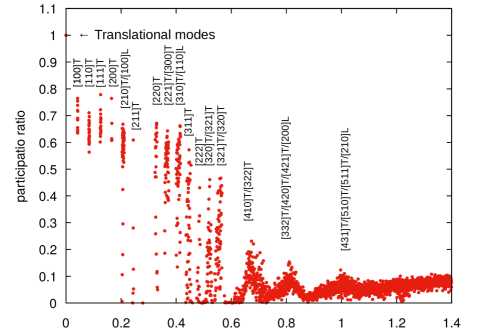
Figure 4: The participation ratio (24) as a function of eigenvalue $\lambda$. At $\lambda=0$, three uniform translational modes exist, having a PR equal to unity. For increasing values of $\lambda$, a bunching of eigenvalues is observed, all of which initially have a PR=2/3, and correspond to eigenmodes which are well described by the plane wave representation $[m,n,l]\Leftrightarrow\bm{k}_{mnl}=2\pi/L(m,n,l)$ of either transverse (T) or longitudinal (L) polarization.

Via Fig. 4, both an eigenvalue and wave-vector magnitude regime can be identified at which the participation ratio rapidly decreases. The large system size presently considered allows us to study this regime in detail, suggesting that a crossover to more heterogeneous modes occurs over a broad range of eigenvalues. This corresponds to length scales of the order of $2\pi/|\bm{k}_{410}|$ to $2\pi/|\bm{k}_{332}|$ and length scales ranging between 20 and 25 bond lengths. Such a length-scale is compatible with amorphous elastic heterogeneity – a length scale which is believed to play a defining role in the break up of sound [32, 24]. Larger system sizes will be needed to investigate whether this cross-over limits to a sharp transition at a distinct length-scale and particular eigenvalue that may be finally identified as the boson peak frequency. It is in such future simulations, that the true power of the current method will become evident since all computational resources can now be focused to the actual eigenvalue region of interest centered around the boson peak frequency.

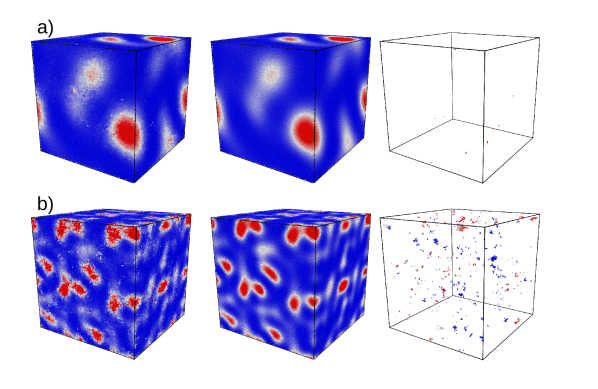
Figure 5: Plots of the amorphous configuration consisting of 1372000 atoms, where each atom is colored according to its value of $|\bm{q}_{i}|^{4}$. The left most panels derive its value from the calculated eigenmode and central panels from the plane wave decomposition. The right-most panels show only those atoms whose oscillator strength significantly deviates from the plane wave decomposition. a) shows a $[110]$ transverse mode, and b) a $[311]$ transverse mode.

5 Conclusions

We have discussed a highly parallel implementation of a polynomial filtered Krylov space-based method for solving large-scale symmetric eigenvalue problems arising in the investigation of amorphous materials. The algorithm enables us to compute hundreds or thousands of eigenvalues of matrices of size in the millions. It the number of eigenvalues is too large to compute at once (e.g. for memory requirement) then the interval of interest can be split in subintervals that contain a reasonable number of eigenvalues whose associated eigenvectors can be accommodated by the available memory.

The polynomial filter is designed to enhance the eigenvalues of the interval of interest. Polynomials of very high degrees result. Therefore, our algorithm is based almost completely on matrix-vector multiplications. The work to keep the basis vectors of the Krylov space orthogonal is negligible. This entails a high potential for parallelization which is confirmed by our experiments.

We plan to apply our solver to problems of size $49^{\prime}152^{\prime}000$ and larger. The use of larger matrices and correspondingly larger simulation cell sizes will give information on how the vibrational modes of the Boson peak regime observed in the present work evolve to the bulk limit. Indeed, the treatment of larger system sizes will result in a transition to a spectrum free of eigenvalue bunching, where the effect of disorder smears the allowed sound-waves into an effectively continuous eigenvalue spectrum. In this experimentally relevant limit, the bulk nature of the Boson peak regime should become manifest from an entirely atomistic description of a model amorphous system.

We will also work on optimizing the evaluation of matrix polynomials, in particular, if the matrix polynomials are applied to multivectors. As noted in (1), $\bm{A}$ is a matrix formed of symmetric $3\times 3$ blocks. In an efficient implementation of the eigensolver this should be taken into account. Doing so, the arithmetic intensity is more than doubled relative to the standard elementwise CRS storage format [7] and execution times can be reduced by about the same factor. Finally, let us note that the abundance of matrix-vector multiplications makes our code amenable to GPU computing.

Appendix A Useful integrals

Here we collect some definite integrals that are needed to compute the coefficients $\gamma_{j}$ in (12) with the function $p$ given in (22). Note that $p$ is a piecewise quadratic polynomial. The integral (25) below has to be evaluated for each of the three subintervals $[a,b]=[\xi-\varepsilon,\xi]$, $[\xi,\eta]$, and $[\eta,\eta+\varepsilon]$, individually.

With $1=T_{0}(x)$, $x=T_{1}(x)$, $2x^{2}=T_{2}(x)+T_{0}(x)$, and the equality [1, eq.(22.7.24)]

$$2T_{m}(x)T_{n}(x)=T_{m+n}(x)+T_{m-n}(x),\qquad m\geq n,$$ (25)

we get

$$\int_{a}^{b}(\alpha+\beta x +\gamma x^{2})T_{j}(x)\frac{dx}{\sqrt{1-x^{2}}}$$ (26)

$$=\int_{a}^{b}\left[(\alpha+\frac{\gamma}{2})T_{0}(x)+\beta T_{1}(x)+\frac{\gamma}{2}T_{2}(x)\right]T_{j}(x)\frac{dx}{\sqrt{1-x^{2}}}$$

$$=\begin{cases}\displaystyle\int_{a}^{b}\left[(\alpha+\frac{\gamma}{2})T_{0}(x)+\beta T_{1}(x)+\frac{\gamma}{2}T_{2}(x)\right]\frac{dx}{\sqrt{1-x^{2}}},&j=0,\\[8.53581pt] \displaystyle\int_{a}^{b}\left[(\alpha+\frac{\gamma}{2})T_{1}(x)+\frac{\beta}{2}(T_{2}(x)+T_{0}(x))+\frac{\gamma}{4}(T_{3}(x)+T_{1}(x))\right]\frac{dx}{\sqrt{1-x^{2}}},&j=1,\\[8.53581pt] \displaystyle\int_{a}^{b}\left[(\alpha+\frac{\gamma}{2})T_{j}(x)+\frac{\beta}{2}(T_{j+1}(x)+T_{j-1}(x))+\frac{\gamma}{4}(T_{j+2}(x)+T_{j-2}(x))\right]\frac{dx}{\sqrt{1-x^{2}}},&j\geq 2.\end{cases}$$

Furthermore, we have

$$\int_{a}^{b}T_{j}(x)\frac{dx}{\sqrt{1-x^{2}}}=-\!\!\int\limits_{\arccos(a)}^{\arccos(b)}\!\!\cos j\vartheta\,d\vartheta=\begin{cases}\arccos(a)-\arccos(b),&j=0,\\[5.69054pt] \frac{\displaystyle\sin(j\arccos(a))-\sin(j\arccos(b))}{\displaystyle j},&j>0.\end{cases}$$ (27)

References

- [1] M. Abramowitz and I. A. Stegun. Handbook of Mathematical Functions. National Bureau of Standards, Washingthon, DC, 10th printing, 1972. Available from http://people.maths.ox.ac.uk/~macdonald/aands/.
- [2] G. Accaputo. Solving large scale eigenvalue problems in amorphous materials. Master’s thesis, ETH Zurich, Computer Science Department, September 2017. doi:10.3929/ethz-b-000221499.
- [3] P. Arbenz, U. L. Hetmaniuk, R. B. Lehoucq, and R. Tuminaro. A comparison of eigensolvers for large-scale 3D modal analysis using AMG-preconditioned iterative methods. Internat. J. Numer. Methods Eng., 64(2):204–236, 2005.
- [4] H. Avron and S. Toledo. Randomized algorithms for estimating the trace of an implicit symmetric positive semi-definite matrix. J. ACM, 58(2):8:1–8:34, 2011.
- [5] C. G. Baker, U. L. Hetmaniuk, R. B. Lehoucq, and H. K. Thornquist. Anasazi software for the numerical solution of large-scale eigenvalue problems. ACM Trans. Math. Softw., 36(3):1–23, 2009.
- [6] M. van Barel. Designing rational filter functions for solving eigenvalue problems by contour integration. Linear Algebra Appl., 502:346–365, 2016.
- [7] R. Barrett, M. Berry, T. F. Chan, J. Demmel, J. Donato, J. Dongarra, V. Eijkhout, R. Pozo, C. Romine, and H. van der Vorst. Templates for the Solution of Linear Systems: Building Blocks for Iterative Methods. SIAM, Philadelphia, PA, 1994. (Available from Netlib at URL http://www.netlib.org/templates).
- [8] C. Bekas, E. Kokiopoulou, and Y. Saad. Polynomial filtered Lanczos iterations with applications in density functional theory. SIAM J. Matrix Anal. Appl., 30(1):397–418, 2008.
- [9] R. J. Bell and P. Dean. Atomic vibrations in vitreous silica. Discuss. Faraday Soc., 50:55–61, 1970.
- [10] L. Berthier, P. Charbonneau, Y. Jin, G. Parisi, B. Seoane, and F. Zamponi. Growing timescales and lengthscales characterizing vibrations of amorphous solids. Proc. Nat. Acad. Sci., 113(30):8397–8401, 2016.
- [11] P. M. Derlet and R. Maaß. Thermal processing and enthalpy storage of a binary amorphous solid: A molecular dynamics study. J. Mater. Res., 32(14):2668–2679, 2017.
- [12] P. M. Derlet and R. Maaß. Local volume as a robust structural measure and its connection to icosahedral content in a model binary amorphous system. Materialia, 3:97–106, 2018.
- [13] P. M. Derlet and R. Maaß. Thermally-activated stress relaxation in a model amorphous solid and the formation of a system-spanning shear event. Acta Mater., 143:205–213, 2018.
- [14] P. M. Derlet, R. Maaß, and J. F. Löffler. The Boson peak of model glass systems and its relation to atomic structure. Eur. Phys. J. B, 85(5):1–20, 2012.
- [15] H.-R. Fang and Y. Saad. A filtered Lanczos procedure for extreme and interior eigenvalue problems. SIAM J. Sci. Comput., 34(4):A2220–A2246, 2012.
- [16] M. Galgon, L. Krämer, B. Lang, A. Alvermann, H. Fehske, A. Pieper, G. Hager, M. Kreutzer, F. Shahzad, G. Wellein, A. Basermann, M. Röhrig-Zöllner, and J. Thies. Improved coefficients for polynomial filtering in ESSEX. In T. Sakurai, S.-L. Zhang, T. Imamura, Y. Yamamoto, Y. Kuramashi, and T. Hoshi, editors, Eigenvalue Problems: Algorithms, Software and Applications in Petascale Computing, pages 63–79. Springer, 2017.
- [17] M. F. Hutchinson. A stochastic estimator of the trace of the influence matrix for Laplacian smoothing splines. Commun. Stat. – Simul. Comput., 19(2):433–450, 1990.
- [18] L. O. Jay, H. Kim, Y. Saad, and J. R. Chelikowsky. Electronic structure calculations for plane-wave codes without diagonalization. Comput. Phys. Comm., 118(1):21 – 30, 1999.
- [19] L. Krämer, E. Di Napoli, M. Galgon, B. Lang, and P. Bientinesi. Dissecting the FEAST algorithm for generalized eigenproblems. J. Comput. Appl. Math., 244:1–9, 2013.
- [20] C. Lanczos. Applied Analysis. Prentice-Hall, Englewood Cliffs, NJ, 1956. (Reprinted by Dover, New York, 1988.).
- [21] R. Li, Y. Xi, E. Vecharynski, C. Yang, and Y. Saad. A thick-restart Lanczos algorithm with polynomial filtering for Hermitian eigenvalue problems. SIAM J. Sci. Comput., 38(4):A2512–A2534, 2016.
- [22] Z. Liang and P. Keblinski. Sound attenuation in amorphous silica at frequencies near the boson peak. Phys. Rev. B, 93(5), 2016.
- [23] L. Lin, Y. Saad, and C. Yang. Approximating spectral densities of large matrices. SIAM Rev., 58(1):34–65, 2016.
- [24] A. Marruzzo, W. Schirmacher, A. Fratalocchi, and G. Ruocco. Heterogeneous shear elasticity of glasses: the origin of the boson peak. Sci. Rep., 3(1407), 2013.
- [25] G. Monaco and S. Mossa. Anomalous properties of the acoustic excitations in glasses on the mesoscopic length scale. Proc. Nat. Acad. Sci., 106(40):16907–16912, 2009.
- [26] E. di Napoli, E. Polizzi, and Y. Saad. Efficient estimation of eigenvalue counts in an interval. Numer. Linear Algebra Appl., 23(4):674–692, 2016.
- [27] B. N. Parlett. The Symmetric Eigenvalue Problem. Prentice Hall, Englewood Cliffs, NJ, 1980. (Republished by SIAM, Philadelphia, 1998.).
- [28] T. J. Rivlin. An Introduction to the Approximation of Functions. Dover, New York, NY, 1981.
- [29] H. Rutishauser. Computational aspects of F. L. Bauer’s simultaneous iteration method. Numer. Math., 13:4–13, 1969.
- [30] Y. Saad. Numerical Methods for Large Eigenvalue Problems. SIAM, Philadelphia, PA, 2nd edition, 2011. (Classics in Applied Mathematics; 66).
- [31] S. Schaffner. Using Trilinos to solve large scale eigenvalue problems in amorphous materials. Master’s thesis, ETH Zurich, Computer Science Department, April 2015.
- [32] W. Schirmacher. The boson peak. Phys. Status Solidi B, 250(5):937–943, 2013.
- [33] W. Schirmacher, G. Ruocco, and T. Scopigno. Acoustic attenuation in glasses and its relation with the boson peak. Phys. Rev. Lett., 98(2), 2007.
- [34] W. Schirmacher, T. Scopigno, and G. Ruocco. Theory of vibrational anomalies in glasses. J. Non-Cryst. Solids, 407:133–140, 2015.
- [35] G. Schofield, J. R. Chelikowsky, and Y. Saad. A spectrum slicing method for the Kohn–Sham problem. Comput. Phys. Comm., 183(3):497–505, 2012.
- [36] H. Shintani and H. Tanaka. Universal link between the boson peak and transverse phonons in glass. Nat. Mat., 7(11):870–877, 2008.
- [37] R. N. Silver and H. Röder. Calculation of densities of states and spectral functions by Chebyshev recursion and maximum entropy. Phys. Rev. E, 56(4):4822–4829, 1997.
- [38] R. N. Silver, H. Röder, A. F. Voter, and J. D. Kress. Kernel polynomial approximations for densities of states and spectral functions. J. Comput. Phys., 124(1):115–130, 1996.
- [39] G. L. G. Sleijpen and J. van den Eshof. On the use of harmonic Ritz pairs in approximating internal eigenpairs. Linear Algebra Appl., 358(1-3):115–137, 2003.
- [40] G. L. G. Sleijpen and H. A. van der Vorst. A Jacobi–Davidson iteration method for linear eigenvalue problems. SIAM J. Matrix Anal. Appl., 17(2):401–425, 1996.
- [41] G. L. G. Sleijpen and H. A. van der Vorst. Jacobi–Davidson method. In Z. Bai, J. Demmel, J. Dongarra, A. Ruhe, and H. van der Vorst, editors, Templates for the solution of Algebraic Eigenvalue Problems: A Practical Guide, pages 238–246. SIAM, Philadelphia, PA, 2000.
- [42] L. N. Trefethen. Approximation Theory and Approximation Practice. SIAM, Philadelphia, PA, 2013.
- [43] The Trilinos Project Home Page. http://trilinos.org/.
- [44] G. Wahnström. Molecular-dynamics study of a supercooled 2-component Lennard–Jones system. Phys. Rev. A, 44(6):3752–3764, 1991.
- [45] A. Weiße, G. Wellein, A. Alvermann, and H. Fehske. The kernel polynomial method. Rev. Mod. Phys., 78:275–306, 2006.
- [46] K. Wu and H. D. Simon. Thick-restart Lanczos method for large symmetric eigenvalue problems. SIAM J. Matrix Anal. Appl., 22(2):602–616, 2000.
- [47] N. Xu, M. Wyart, A. J. Liu, and S. R. Nagel. Excess vibrational modes and the Boson peak in model glasses. Phys. Rev. Lett., 98(17), 2007.
- [48] I. Yamazaki, H. Tadano, T. Sakurai, and T. Ikegami. Performance comparison of parallel eigensolvers based on a contour integral method and a Lanczos method. Parallel Comput., 39(6):280–290, 2013.
- [49] Y. Zhou, Y. Saad, M. L. Tiago, and J. R. Chelikowsky. Self-consistent field calculations using Chebyshev-filtered subspace iteration. J. Comput. Phys., 219(1):172–184, 2006.