Employing latent variable models to improve efficiency in composite endpoint analysis

Abstract

Composite endpoints that combine multiple outcomes on different scales are common in clinical trials, particularly in chronic conditions. In many of these cases, patients will have to cross a predefined responder threshold in each of the outcomes to be classed as a responder overall. One instance of this occurs in systemic lupus erythematosus (SLE), where the responder endpoint combines two continuous, one ordinal and one binary measure. The overall binary responder endpoint is typically analysed using logistic regression, resulting in a substantial loss of information. We propose a latent variable model for the SLE endpoint, which assumes that the discrete outcomes are manifestations of latent continuous measures and can proceed to jointly model the components of the composite. We perform a simulation study and find the method to offer large efficiency gains over the standard analysis. We find that the magnitude of the precision gains are highly dependent on which components are driving response. Bias is introduced when joint normality assumptions are not satisfied, which we correct for using a bootstrap procedure. The method is applied to the Phase IIb MUSE trial in patients with moderate to severe SLE. We show that it estimates the treatment effect 2.5 times more precisely, offering a 60% reduction in required sample size. Latent variable models; Composite endpoints; Responder analysis; Systemic lupus erythematosus

1 Introduction

Composite endpoints combine multiple outcomes in order to determine the effectiveness or efficacy of a treatment for a given disease. They are typically recommended when a disease is complex or multi-system and meaningful improvement cannot be captured in a single outcome. Furthermore, the endpoint may be a combination of continuous and discrete outcomes which are collapsed in to a single binary responder index.
Table 1 shows examples of diseases that use composite endpoints combining multiple continuous and discrete components. Responders in fibromyalgia must respond in two continuous and one ordinal component however responders in trials for frailty or soft tissue infections must respond in a total of five continuous and discrete components. Generally, these composite responder endpoints will be treated as a single binary outcome and analysed using a logistic regression model, which we term the standard binary method. This solves problems with multiplicity however results in large losses in efficiency (Wason and Seaman (2013)). The aim of this paper is to propose a joint modelling framework within which we can model the components of the composite, retaining the information on the original scales of the outcomes, hence increasing efficiency.

Table 1: Examples of diseases that use complex composite endpoints combining multiple discrete and continuous measures to determine effectiveness of a treatment including criteria for response and how each component is measured

Disease	Responder endpoint	Measured by
Fibromyalgia	•  achieved a 30% improvement in	Electronic diary
	pain
	•  30% improvement in functional	Subscale of Fibromyalgia Impact
	status	Questionnaire (FIQ)
	•  improved, much improved, or	7-point Patient Global Impression of
	very much improved	Change (PGIC) scale
Frailty	•  BMI$<$18.5 kg/m2 OR $>$10%	weight and height
	weight loss since last wave
	•  One positive answer to exhaustion	CES-D questionnaire
	questions
	•  Low grip strength (M $<$ 31.12 kg,	Eg. Jamar hand dynamometer
	F $<$ 17.60 kg)
	•  Gait speed (M $<$ 0.691 m/s,	Distance/time
	F $<$ 0.619 m/s)
	•  Low activity (M $<$ 16.5 activity	Activity units derived using intensity
	units, F $<$ 13.5 activity units)	vs. frequency
Necrotizing	•  Alive until day 28	yes/no
Soft Tissue	•  Day 14 debridements $\leq$ 3	surface area
Infections	•  No amputation if debridement	yes/no
	•  Day 14 mSOFA score $\leq$ 1	mSOFA score - composite additively
		combining scores in different systems
	•  Reduction of at least 3 score	mSOFA score - composite additively
	points in mSOFA score	combining scores in different systems
Systemic lupus	•  Change in SLEDAI $\leq$ -4	SLE Disease Activity Index
erythematosus	•  Change in PGA $<$ 0.3	Physicians Global Assessment
	•  No Grade A or more than one	British Isles Lupus Assessment Group
	Grade B in BILAG
	•  Reduction in oral corticosteroids	Notes

One likelihood based method for handling mixed data is the factorisation model. The objective is to factorise the joint distribution and fit a univariate model to each component of the factorisation (de Leon and Carriere (2013)). This accounts for correlations between the outcomes by including one response as a covariate in the model for the other response. In the graphical modelling literature this has been termed the ‘Conditional Gaussian Distribution’ (Whittaker (1990); Lauritzen and Wermuth (1989)). An advantage of these methods in relation to the composite endpoint problem is that we may account for correlations between measurements whilst making inference directly on the outcomes that we have measured, hence they fall within a broader class of ‘direct methods’. Examples of applications of these ideas, which build on the work of Olkin and Tate (1961), include developmental toxicity studies by Fitzmaurice and Laird (1995) and in the longitudinal setting, the augmented binary method was developed for application to composite endpoints in clinical trials where the composite is formed of one continuous and one binary outcome (Wason and Seaman (2013); Wason and Jenkins (2016); McMenamin and others (2018)). One difficulty with these methods beyond the bivariate scenario is the range of possibilities for the factorisations, with no consensus on how this should be determined. In the case of the SLE responder endpoint with four components, this amounts to 24 possible factorisations, each of which may result in different conclusions (Verbeke and others (2014); de Leon and Carriere (2013)).
Another family of models used to model mixed outcome types which feature frequently in economics and finance are copulas. These are functions that join or couple multivariate distribution functions to their uniform one-dimensional marginal distribution functions as discussed by Nelsen (1999). Copulas offer a flexible framework in this setting, as the marginal distribution functions need not come from the same parametric family. While the construction of copulas is considered to be mathematically elegant and the flexibility with which we can model appealing, they are not without their shortcomings. Extensions beyond the bivariate setting are difficult and have failed to perform well in many applications (de Leon and Carriere (2013)). Other practical implications include poor out-of-sample predictions due to the wide variety of copulas available. These restrictions, along with difficulties in longitudinal settings with unbalanced data structures, have seen few applications of copulas for mixed outcome types in the medical statistics literature (Verbeke and others (2014)). Applications of copulas in mixed outcome settings include de Leon and Wu (2010) and Wu and de Leon. A.R. (2014).
Another likelihood based method that allows for more flexibility when modelling the correlations between outcomes falls within the framework of latent variable models (Skrondal and Rabe-Hesketh (2004)). The multiple outcomes are assumed to be physical manifestations of some underlying latent process. This is modelled by including the same latent variable in each of the models for the observed responses. The outcomes are then assumed to be independent conditional on this latent variable. This solves the problem of deciding the order of factorisations in previously discussed methods however this formulation results in the inclusion of some covariance parameters in the mean structure, leaving the model sensitive to misspecification of the correlation structure (Sammel and Ryan (2002)). One example of these models is introduced by Sammel and others (1997), where effects of covariates of interest are modelled through this shared latent variable. Although these models have the intuitive interpretation that each outcome is attempting to capture underlying disease activity, the correlation matrix is restricted to allow for the same correlation between each pair of outcomes, which is unlikely in practice. This structure is relaxed in work by Dunson (2000), where the effects of covariates are included in the model separately from the latent variable. The correlation structure can be further relaxed to allow for a different latent variable for each outcome, meaning that pairs of outcomes are not assumed to have the same correlation. However these models would require integrating out each of the latent variables in order to obtain the joint distribution of interest (McCulloch (2008)). Furthermore, they are relevant in applications with multiple time points however less so for a single time point, as is the case for the composite endpoint problem.
Latent variables have also been used in the setting of mixed continuous and discrete variables to a different end. Namely, the outcomes adopt a correlated Gaussian distribution by assuming that the discrete outcomes are coarsely measured manifestations of underlying continuous variables subject to some threshold specifications, as seen in Ashford and Sowden (1970) and Chib and Greenberg (1998). Specifying discrete variables in terms of a partitioning of the latent variable space into non-overlapping intervals dates back to Pearson (1904) in relation to his generalised theory of alternative inheritance and has received much consideration in the literature since. Terminology surrounding these models is inconsistent but they are often referred to as multivariate probit models (Ashford and Sowden (1970)). This theory can also be found to underpin conditional grouped continuous models (Poon and Lee (1987)). By formulating the distribution in this way, we can correlate the error terms between models and work within the familiar paradigm of Gaussian distributions and maximum likelihood theory. The theory and application of these ideas for a mixture of continuous and binary outcomes has featured in the statistics literature, see for example work by Tate (1955), Cox and Wermuth (1992) and Catalano and Ryan (1992). Generalisations of these ideas, which appear less frequently in the literature, lead to methods for modelling continuous and ordinal variables, with applications in developmental toxicology (Catalano (1997); Samani and Ganjali (2008); Arminger and Kusters (1988); Regan and Catalano (2000); Faes and others (2002)). Despite the advantages, the multivariate probit model has not realised its full potential in the applied biostatistics literature. This was noted by Lessafre and Molenberghs (1991) and we believe it still to be the case today. The few applications that do appear tend to demonstrate bivariate scenarios or those that mix continuous and binary or continuous and ordinal, rather than all three. Furthermore, these models have not been considered specifically to address challenges with modelling composite endpoints. Other work has combined thresholding the response variables and introducing latent variables in the model, examples include work by Gueorguieva and Agresti (2001), de Leon and Carriere (2013), Gueorguieva and Sanacora (2003) and Gueorguieva and Sanacora (2006), however these ideas are most applicable in the longitudinal setting. We will therefore employ the latent outcome framework and investigate its use for the composite endpoint problem.
The paper proceeds as follows. In Section 2 we discuss systemic lupus erythematosus (SLE), the motivating example for the methods. In Section 3 we introduce the latent variable model and discuss how we conduct estimation and inference. In Section 4 we compare the behaviour of the latent variable model with the augmented binary and standard binary methods, including the case when the key assumptions are not satisfied. In Section 5 we apply the methods to the Phase IIb MUSE trial in patients with moderate to severe SLE. Finally, in Section 6 we discuss our findings and make some recommendations.

2 Motivating example

In what follows we will focus specifically on systemic lupus erythematosus (SLE), however the methods introduced will be relevant to other diseases using endpoints with a similar structure. The SLE endpoint is shown in Figure 1. It combines a continuous PGA measure, a continuous SLEDAI measure, an ordinal BILAG measure and a binary corticosteroids measure, where patients must meet the response criteria in all components in order to be classed as a responder overall. Note that the SLEDAI and BILAG measures are themselves composite scores deriving from a combination of items, however this will not be considered in the analysis.
The real data underpinning this motivation comes from the MUSE study (Furie and others (2017)). It was a Phase IIb, randomised, double-blind, placebo-controlled study investigating the efficacy and safety of anifrolumab in adults with moderate to severe SLE. Patients (n=305) were randomised to receive anifrolumab (300mg or 1000mg) or placebo, in addition to standard therapy every 4 weeks for 48 weeks. The primary end point was the percentage of patients achieving an SRI response at week 24 with sustained reduction of oral corticosteroids ($<$10mg/day and less than or equal to the dose at week 1 from week 12 through 24). The methods discussed will make inference at one time point, as this is the case in the trial, although they can be easily extended for the longitudinal case.

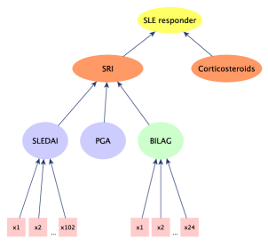
Figure 1: Structure of the composite endpoint use in trials of systemic lupus erythematosus. The continuous SLEDAI, continuous PGA and ordinal BILAG measures are dichotomised and combined to form the binary SRI indicator which is then combined with the binary taper variable to form the overall binary SLE responder index

3 Methods

3.1 Notation

Let $\mathbf{Y}_{i}=(Y_{i1},Y_{i2},Y_{i3}^{*},Y_{i4}^{*})$ represent the vector of observed and latent continuous measures for patient i. $Y_{i1}$ and $Y_{i2}$ are the observed continuous SLEDAI and PGA measures. Let $Y_{i3}$ denote BILAG, the observed ordinal manifestation of $Y_{i3}^{*}$ and $Y_{i4}$ the observed binary taper variable for $Y_{i4}^{*}$. $T_{i}$ represents the treatment indicator for patient i, $y_{i10}$ and $y_{i20}$ are the baseline measures for $Y_{i1}$ and $Y_{i2}$ respectively.

3.2 Model

The mean structure for the outcomes is shown in (1). The baseline measures $y_{10}$ and $y_{20}$ are included in the model for $Y_{1}$ and $Y_{2}$ respectively.

$$\begin{split}Y_{i1}&=\alpha_{0}+\alpha_{1}T_{i}+\alpha_{2}y_{i10}+\varepsilon_{i1}\\ Y_{i2}&=\beta_{0}+\beta_{1}T_{i}+\beta_{2}y_{i20}+\varepsilon_{i2}\\ Y_{i3}^{*}&=\gamma_{1}T_{i}+\varepsilon_{i3}^{*}\\ Y_{i4}^{*}&=\psi_{0}+\psi_{1}T_{i}+\varepsilon_{i4}^{*}\end{split}$$ (1)

The observed discrete variables are related to the latent continuous variables by partitioning the latent variable space, as shown in (2). The lower and upper thresholds for both discrete variables are set at $\tau_{03}=\tau_{04}=-\infty,\tau_{53}=\tau_{24}=\infty$. The intercept term for the ordinal variable in (1) is set at $\gamma_{0}=0$ so that the cut-points $\tau_{13},\tau_{23},\tau_{33},\tau_{43}$ may be estimated. The intercept for the binary outcome $\psi_{0}$ may be estimated, as $\tau_{14}=0$.

$$Y_{i3}=\begin{cases}$ Grade E$&\text{if }\tau_{03}\leq Y_{i3}^{*}<\tau_{13},\\ $ Grade D $&\text{if }\tau_{13}\leq Y_{i3}^{*}<\tau_{23},\\ $ Grade C$&\text{if }\tau_{23}\leq Y_{i3}^{*}<\tau_{33},\\ $ Grade B $&\text{if }\tau_{33}\leq Y_{i3}^{*}<\tau_{43},\\ $ Non-responder$&\text{if }\tau_{43}\leq Y_{i3}^{*}<\tau_{53}\end{cases} Y_{i4}=\begin{cases}0,&\text{if }\tau_{04}\leq Y_{i4}^{*}<\tau_{14},\\ 1,&\text{if }\tau_{14}\leq Y_{i4}^{*}<\tau_{24}\end{cases}$$ (2)

Following these assumptions, we can model the error terms in (1) as multivariate normal with zero mean and variance-covariance matrix $\Sigma$, as shown in (3). Note that the error variances for $\varepsilon_{3}^{*},\varepsilon_{4}^{*}$ are $\sigma_{3}=1$ and $\sigma_{4}=1$. This does not represent a constraint on the model but rather a rescaling required for identifiability.

$$(\varepsilon_{i1},\varepsilon_{i2},\varepsilon_{i3}^{*},\varepsilon_{i4}^{*})\sim N(0,\Sigma) \Sigma=\begin{pmatrix}\sigma_{1}^{2}&\rho_{12}\sigma_{1}\sigma_{2}&\rho_{13}\sigma_{1}&\rho_{14}\sigma_{1}\\ \rho_{12}\sigma_{1}\sigma_{2}&\sigma_{2}^{2}&\rho_{23}\sigma_{2}&\rho_{24}\sigma_{2}\\ \rho_{13}\sigma_{1}&\rho_{23}\sigma_{2}&1&\rho_{34}\\ \rho_{14}\sigma_{1}&\rho_{24}\sigma_{2}&\rho_{34}&1\end{pmatrix}$$ (3)

Subsequently, we may factorise the joint likelihood contribution for patient i as shown below.

$$l(\boldsymbol{\theta};\mathbf{Y})=f(Y_{i1},Y_{i2};\boldsymbol{\theta})f(Y_{i3}^{*},Y_{i4}^{*}|Y_{i1},Y_{i2};\boldsymbol{\theta})$$ (4)

where $\boldsymbol{\theta}$ is a vector which contains all model parameters. The observed likelihood can then be expressed as in (5).

$$l(\boldsymbol{\theta};\mathbf{Y})=\prod_{i=1}^{n}\prod_{w=1}^{5}\prod_{k=1}^{2}f(Y_{i1},Y_{i2};\boldsymbol{\theta})\left[pr\left(Y_{i3}=w,Y_{i4}=k|Y_{i1}=y_{i1},Y_{i2}=y_{i2};\boldsymbol{\theta}\right)\right]^{I\{Y_{i3}=w,Y_{i4}=k\}}$$ (5)

The joint probability of patients having discrete measurements $Y_{i3}=w$ and $Y_{i4}=k$ must be multiplied over the five ordinal levels and two binary levels resulting in ten combinations of the probabilities in (6) to be calculated. We discuss the intuition for (6) in Appendix A.

$$pr\left(Y_{i3}=w,Y_{i4}=k|Y_{i1}=Y_{i1},Y_{i2}=Y_{i2};\boldsymbol{\theta}\right)=\\ \Phi_{2}\left(\tau_{w3}-\mu_{3|1,2},\tau_{k4}-\mu_{4|1,2};\Sigma_{3,4|1,2}\right)-\Phi_{2}\left(\tau_{(w-1)3}-\mu_{3|1,2},\tau_{k4}-\mu_{4|1,2};\Sigma_{3,4|1,2}\right)-\\ \Phi_{2}\left(\tau_{w3}-\mu_{3|1,2},\tau_{(k-1)4}-\mu_{4|1,2};\Sigma_{3,4|1,2}\right)+\Phi_{2}\left(\tau_{(w-1)3}-\mu_{3|1,2},\tau_{(k-1)4}-\mu_{4|1,2};\Sigma_{3,4|1,2}\right)$$ (6)

where $\Phi_{2}$ is the bivariate standard normal distribution function and $\mu_{3|1,2},\mu_{4|1,2}$ and $\Sigma_{3,4|1,2}$ are derived using the rules of conditional multivariate normality, resulting in (7).

$$\begin{split}\mu_{3|1,2}=&\mu_{3}+\tfrac{\left(\rho_{13}-\rho_{12}\rho_{23}\right)}{\sigma_{1}\left(1-\rho_{12}^{2}\right)}\left(Y_{i1}-\mu_{1}\right)+\tfrac{\left(\rho_{23}-\rho_{12}\rho_{13}\right)}{\sigma_{2}\left(1-\rho_{12}^{2}\right)}\left(Y_{i2}-\mu_{2}\right)\\ \mu_{4|1,2}=&\mu_{4}+\tfrac{\left(\rho_{14}-\rho_{12}\rho_{24}\right)}{\sigma_{1}\left(1-\rho_{12}^{2}\right)}\left(Y_{i1}-\mu_{1}\right)+\tfrac{\left(\rho_{24}-\rho_{12}\rho_{14}\right)}{\sigma_{2}\left(1-\rho_{12}^{2}\right)}\left(Y_{i2}-\mu_{2}\right)\end{split}$$ (7)

$$\Sigma_{3,4|1,2}=\begin{pmatrix}1-\frac{\rho_{13}^{2}-2\rho_{12}\rho_{13}\rho_{23}+\rho_{23}^{2}}{1-\rho_{12}^{2}}&\rho_{34}-\frac{\rho_{13}\rho_{14}-\rho_{12}\rho_{13}\rho_{24}-\rho_{12}\rho_{14}\rho_{23}+\rho_{23}\rho_{24}}{1-\rho_{12}^{2}}\\ \rho_{34}-\frac{\rho_{13}\rho_{14}-\rho_{12}\rho_{13}\rho_{24}-\rho_{12}\rho_{14}\rho_{23}+\rho_{23}\rho_{24}}{1-\rho_{12}^{2}}&1-\frac{\rho_{14}^{2}-2\rho_{12}\rho_{14}\rho_{24}+\rho_{24}^{2}}{1-\rho_{12}^{2}}\end{pmatrix}$$

3.3 Estimation

As the variance parameters $(\sigma_{1},\sigma_{2})$ are required to be greater than 0, we introduce parameters $(\delta_{1},\delta_{2})$ such that $\sigma_{1}=exp(\delta_{1})$ and $\sigma_{2}=exp(\delta_{2})$. This transformation ensures that the variance is above 0 whilst allowing the parameter we estimate to take any real value. We must also ensure that the correlation parameters $(\rho_{12},\rho_{13},\rho_{14},\rho_{23},\rho_{24},\rho_{34})$ are estimated within (-1,1) by introducing $(\delta_{12},\delta_{13},\delta_{14},\delta_{23},\delta_{24},\delta_{34})$, where $\rho_{12}=2expit(\delta_{12})-1,\rho_{13}=2expit(\delta_{13})-1,\rho_{14}=2expit(\delta_{14})-1,\rho_{23}=2expit(\delta_{23})-1,\rho_{24}=2expit(\delta_{24})-1,\rho_{34}=2expit(\delta_{34})-1$.
We fit the model in R by coding the likelihood function, probability of response and using the delta method to obtain standard errors. The bivariate distribution functions in (6) are estimated using ‘pmvnorm’, using the method of Genz (1992). The likelihood maximisation is conducted using the ‘nlminb’ function in the ‘optimx’ package, which is the best performing method in terms of accuracy and convergence rate, however is the slowest. We use the ‘Hessian’ function in the ‘numDeriv’ package to obtain the Hessian matrix and invert this to get the covariance matrix of the model parameters. In a small number of cases the Hessian is not positive definite because of computational error, meaning that it cannot be inverted. This is rectified in these cases by using the ‘near PD’ function in the ‘Matrix’ package, which computes the nearest positive definite matrix.

3.4 Inference

We wish to make inference on the probability of response. Let $S_{i}$ be an indicator for patient i denoting whether or not they achieved response defined by $S_{i}$=1 if $Y_{i1}\leq\theta_{1},Y_{i2}\leq\theta_{2},Y_{i3}^{*}\leq\theta_{3},Y_{i4}^{*}\leq\theta_{4}$. Therefore,

$$P(S_{i}=1\mid T_{i},y_{i10},y_{i20})=\int_{-\infty}^{\theta_{1}}\int_{-\infty}^{\theta_{2}}\int_{-\infty}^{\theta_{3}}\int_{-\infty}^{\theta_{4}}f_{\mathbf{Y}}(\mathbf{Y};T_{i},y_{i10},y_{i20})dy_{i4}^{*}dy_{i3}^{*}dy_{i2}dy_{i1}$$ (8)

We obtain the integrand in (8) by using the fitted values of the parameters in the conditional mean and conditional covariance matrix in (7). Parameter estimates from these methods are maximum likelihood estimates and so we avail of asymptotic maximum likelihood theory. The integral in (8) is evaluated using the ‘R2Cuba’ package to obtain estimates for each patient, assuming they were treated $\tilde{p_{i1}}$ and not treated $\tilde{p_{i0}}$. The odds ratio treatment effect is then defined as shown in (9).

$$\tilde{\delta}=\dfrac{\left(\dfrac{\sum_{i=1}^{N}{\tilde{p_{i1}}}}{N-\sum_{i=1}^{N}{\tilde{p_{i1}}}}\right)}{\left(\dfrac{\sum_{i=1}^{N}{\tilde{p_{i0}}}}{N-\sum_{i=1}^{N}{\tilde{p_{i0}}}}\right)}$$ (9)

Note that we can easily define a risk difference or risk ratio using these quantities but in what follows we consider $\tilde{\delta}$ to be the effect of interest. The standard error estimates are obtained using the delta method. This requires the covariance matrix of the maximum likelihood estimates Cov($\boldsymbol{\hat{\theta}}$) and ${}^{\prime\prime}\tilde{\boldsymbol{\delta}}$, the vector of partial derivatives of $\tilde{\delta}$ with respect to each of the parameter estimates. The variance of $\tilde{\delta}$ is obtained as shown in (10).

$$Var(\tilde{\delta})=(^{\prime\prime}\tilde{\boldsymbol{\delta}})^{T}Cov(\boldsymbol{\hat{\theta}})(^{\prime\prime}\tilde{\boldsymbol{\delta}})$$ (10)

Alternatively, the quantity in (8) can also be considered to be a multivariate Gaussian hidden truncation distribution, from which we can obtain a closed form solution, and proceed as detailed by Arnold (2009).
Another important consideration for the model is how to assess goodness-of-fit. We propose an extension to an existing method for application in this case, which is detailed in Appendix B in the supplementary material.

4 Simulation study

We are interested in comparing the performance of the latent variable, augmented binary and standard binary methods through simulation. The models for the augmented binary and standard binary methods are included in Appendix C in the supplementary material.

4.1 Data generating model

Initially, we investigate the properties of the methods when the assumptions of the latent variable model are satisfied. The parameter values in the ‘baseline’ scenario are chosen to simulate a scenario where composite endpoints are typically recommended for use. Namely, that all four components drive response and items are correlated but not so highly that the composite becomes redundant. The parameter values have been informed by the MUSE trial dataset, in particular the correlation structure. The response probability in the control arm is 0.275 and in the treatment arm is 0.381, resulting in an odds ratio equal to 1.6, values typically observed in trials requiring response in all four components. The parameter values selected for the model in (1) are shown in Table 2. From this baseline case, we vary parameters to determine how the methods behave under various scenarios of interest. In particular, under varying treatment effect, varying responder threshold and varying drivers of response. The parameter values for these data generating models are included in Appendix D in the supplementary material.

Table 2: Parameter values for the data generating model in the baseline simulation scenario comparing the performance of the latent variable, augmented binary and standard binary methods for analysing a composite endpoint, where the values correspond to a treatment effect in all components and all components drive response

Purpose	Values
Total sample size	N=300
Intercept	$\alpha_{0}=-4.9,\beta_{0}=-1.2,\psi_{0}=-0.2$
Treatment	$\alpha_{1}=-0.28,\beta_{1}=-0.35,\gamma_{1}=-0.24,\psi_{1}=-0.18$
Baseline value	$\alpha_{2}=-0.5,\beta_{2}=-0.5$
Variance	$\sigma_{1}=\sigma_{2}=1$
Correlation	$\rho_{12}=0.5,\rho_{13}=\rho_{24}=0.35,\rho_{14}=0.25,\rho_{23}=0.4,\rho_{34}=0.3$
Discrete cut-point	$\tau_{13}=-1,\tau_{23}=-0.1,\tau_{33}=0.45,\tau_{43}=1.3$
Responder threshold	$\theta_{1}=-4,\theta_{2}=-0.6,\theta_{3}=0.45,\theta_{4}=0$

4.2 Results

The methods are evaluated against a range of performance criteria, which are included with their Monte Carlo standard errors in Appendix E of the supplementary material. For further details see Morris and others (2017).

4.2.1 Varying treatment effect

Figure 2 shows the bias of the methods as the treatment effect varies. The standard binary method is unbiased, as we would expect for a logistic regression in a large sample. The latent variable method is unbiased for smaller treatment effects but a small bias towards the null is introduced as the treatment effect increases. The augmented binary method is biased away from the null in this setting and the bias increases as the treatment effect increases. Given that this performance is worse than is suggested from previous applications of the augmented binary method in Wason and Seaman (2013) and Wason and Jenkins (2016), this would suggest that the treatment effect from the augmented binary method may be biased if the model is misspecified.

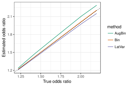
Figure 2: Bias reported from the latent variable method, augmented binary method and standard binary method when $n_{sim}$=5000, total sample size N=300 for true log-odds treatment effect between 1.2 and 2.2. The composite endpoint of interest contains four components: two continuous, one ordinal, one binary and treatment effects are present in all four components

The coverage of the methods is shown in Figure 3. The binary method has approximately nominal coverage. The latent variable method has nominal coverage for smaller treatment effects, however the coverage probability decreases as the treatment effect increases. The augmented binary method has coverage of approximately 0.91, which also decreases when the treatment effect increases.

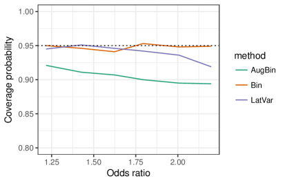
Figure 3: Coverage probability reported from the latent variable method, augmented binary method and standard binary method for $n_{sim}$=5000, total sample size N=300 for true log-odds treatment effect between 1.2 and 2.2. The composite endpoint of interest contains four components: two continuous, one ordinal, one binary and treatment effects are present in all four components

In order to diagnose this under-coverage in the joint modelling methods we can look at bias-corrected coverage, as recommended in Morris and others (2017). Figure 4 shows both the coverage and bias-corrected coverage for the three methods. The properties of the standard binary method remain unchanged. The bias-corrected coverage of the latent variable method is 0.95, which indicates that any under-coverage is due to the bias present. This is not true for the augmented binary method which shows small improvements in bias-corrected coverage, indicating that under-coverage is present in this method due to reasons other than bias. Again, this may be down to model misspecification.

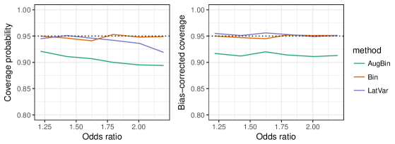
Figure 4: Coverage probability (left) and bias-corrected coverage probability (right) reported from the latent variable method, augmented binary method and standard binary method for $n_{sim}$=5000, total sample size N=300 for true log-odds treatment effect between 1.2 and 2.2. The composite endpoint of interest contains four components: two continuous, one ordinal, one binary and treatment effects are present in all four components

The power of the three methods is shown in Figure 5. The performance of the binary and augmented binary methods are as we would expect based on previous findings in Wason and Seaman (2013) and Wason and Jenkins (2016). The latent variable method offers much higher power. In this setting it has close to 100% power for odds ratios larger than 1.6, an effect that is plausible to observe in a trial.

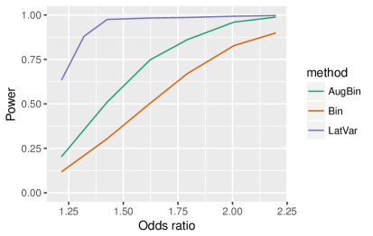
Figure 5: Statistical power reported from the latent variable method, augmented binary method and standard binary method for $n_{sim}$=5000, total sample size N=300 for true log-odds treatment effect between 1.2 and 2.2. The composite endpoint of interest contains four components: two continuous, one ordinal, one binary and treatment effects are present in all four components

These findings have indicated that the standard binary method has the smallest bias and that the latent variable method has the smallest variance. The mean squared error (MSE) provides a combined measure of bias and variance. Figure 6 shows the MSE of the three methods as the treatment effect varies. The MSE for the standard and augmented binary methods is approximately 6.5 times that of the latent variable method. However, this measure should be interpreted with care due to the fact that the MSE is more sensitive to the sample size than comparisons of bias or empirical SE alone (Morris and others (2017)).

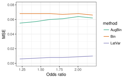
Figure 6: Mean Squared Error (MSE) reported from the latent variable method, augmented binary method and standard binary method for $n_{sim}$=5000, total sample size N=300 for true log-odds treatment effect between 1.2 and 2.2. The composite endpoint of interest contains four components: two continuous, one ordinal, one binary and treatment effects are present in all four components

4.2.2 Varying $\theta_{1}$

To understand more about the precision performance of the augmented binary method in particular, we vary the responder threshold $\theta_{1}$ to change the proportion of responders in that outcome. Figure 7 shows the density of the $Y_{1}$ variable and the relative precision of the methods, as the responder threshold varies. The precision gains from the augmented binary method diminish as the threshold increases. This is intuitive, as improvements in efficiency fall as the continuous component becomes less responsible for driving response. It is interesting to note that all precision gains are lost for any thresholds above -4. Therefore, even when 20% of patients are non-responders, all efficiency gains are lost. The percentage of responders needed to improve efficiency using the augmented binary method will of course depend on the correlation structure employed. Due to the additional information in the other components, the latent variable method is still five times as precise as the other methods.

Figure 7: Density of continuous $Y_{1}$ variable (left) and estimated relative precision of augmented binary versus standard binary method, latent variable versus augmented binary method and latent variable versus standard binary method as the $Y_{1}$ responder threshold $\theta_{1}$ varies between $\theta_{1}=-6$ and $\theta_{1}=-2$ (right) for $n_{sim}$=5000 and total sample size N=300. The composite endpoint of interest contains four components: two continuous, one ordinal, one binary and treatment effects are present in all four components

4.2.3 Components contributing to response

An important consideration when investigating performance is how the precision changes when different combinations of outcomes are responsible for driving response. Figure 8 shows boxplots of the relative precision for the methods for four different response combinations, namely when response is driven by $(Y_{1},Y_{2},Y_{3},Y_{4}),(Y_{1},Y_{2},Y_{3}),(Y_{1},Y_{4})$ and $(Y_{4})$, where $Y_{1}$ and $Y_{2}$ are observed as continuous variables, $Y_{3}$ is ordinal and $Y_{4}$ is binary.

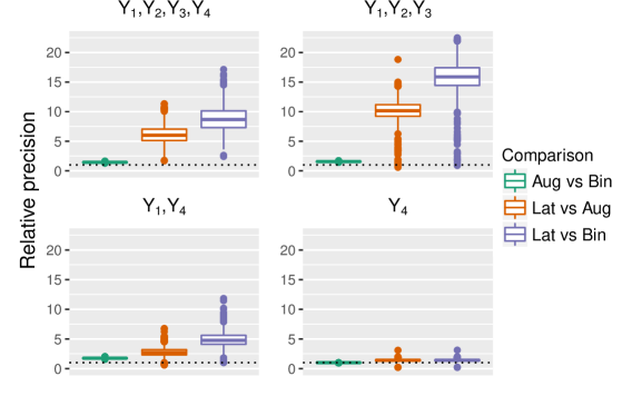
Figure 8: Estimated relative precision gains from augmented binary versus standard binary method, latent variable versus augmented binary method and latent variable versus standard binary method when different combinations of components driving response. Response driven by $Y_{1},Y_{2},Y_{3},Y_{4}$ (top left), $Y_{1},Y_{2},Y_{3}$ (top right), $Y_{1},Y_{4}$ (bottom left) and $Y_{4}$ (bottom right) where $Y_{1},Y_{2}$ are continuous, $Y_{3}$ is ordinal, $Y_{4}$ is binary for $n_{sim}$=5000 and total sample size N=300. The composite endpoint of interest contains four components: two continuous, one ordinal, one binary and treatment effects are present in all four components

When all four components contribute to response, the latent variable method outperforms the other methods, offering large precision gains. The variability in the magnitude of these gains is large, with the median result showing that the latent variable method reports the treatment effect 8 times more precisely than the binary method and 6 times more precisely than the augmented binary method. If response is driven by $(Y_{1},Y_{2},Y_{3})$ then the relative median gains for the latent variable method are larger, however note that in less that 2% of cases the treatment effect is reported equally or less precisely than from both of the other methods. The findings are similar when response is driven by $(Y_{1},Y_{4})$, however the median gains are much smaller. The treatment effect is reported 5 times more precisely from the latent variable method than the binary method in this setting. Note that as the augmented binary method models the relevant components it still performs well and again better than the latent variable method in a very small number of cases. When binary $Y_{4}$ determines response, the augmented binary method offers no improvement in precision whereas the latent variable method is approximately 1.5 times more precise. It is clear from the results that the magnitude of the precision gains from the latent variable method is highly dependent on the structure of the data.

4.3 Sensitivity analysis

The key assumptions in this model are that of joint normality of the four components and that the discrete variables are realisations of latent continuous variables. Although it is not possible to test these assumptions in real data, we can investigate how robust the latent variable method is to deviations from these conditions. We can do this by drawing from the multivariate skew-normal distribution with different degrees of skew in each of the components. The first scenario investigated considers when all four components are skewed. Scenarios 2-3 consider different magnitudes of skew in the latent continuous components only. This tests the robustness of the method to the assumption that the observed discrete variables manifest from a true normal continuous variable. Scenario 4 is the null case for scenario 3. The results are shown in Appendix F of the supplementary material.

In summary, scenarios 1-3 have increased bias resulting in under-coverage as the bias-corrected coverage is close to nominal for all scenarios. The coverage of the latent variable method is nominal in the null case. This is consistent with our previous findings however the magnitude of the bias is much smaller when the assumptions are satisfied. The latent variable method still offers large power gains over the other methods. The MSE is smallest for the latent variable method across all scenarios investigated, indicating that the large reduction in variance is useful despite the introduction of bias. The latent variable method estimates the probability of response in the control arm well however underestimates the probability of response in the treatment arm. The magnitude of this underestimation is unaffected by the degree of skew or whether the skew is present in the observed continuous components. The relative precision of the methods are consistent with our previous findings indicating that the violation of joint normality only affects the bias and not the variance. The augmented binary and standard binary methods behave similarly to when the joint normality assumptions are satisfied, which is expected given that the assumptions of those models are violated in both contexts.

5 Case study

5.1 Data structure

Due to data sharing policy, we conduct the analysis for a subset of the patients, N=278 rather than N=305 reported in the paper, so the results will differ from the original paper. Furthermore, only the anifrolumab 300mg arm (n=95) and the placebo arm (n=87) will be used to illustrate the methods.
The simulation results have suggested that the structure of the data is important for how the methods will perform, in particular the magnitude of the precision gains depends highly on which components drive response. Table 3 shows the criteria for response in each component and the rates of response in each by treatment arm. This suggests that the components responsible for responder discrimination are the continuous SLEDAI measurement and the binary taper measure.

Table 3: Observed response rates in each of the SLE responder index components in the anifrolmab 300mg arm and placebo arm of the Phase IIb MUSE trial. SLE index is comprised of a continuous SLEDAI outcome, continuous PGA outcome, ordinal BILAG outcome and binary taper outcome where response in each component is achieved when the patient meets the criteria shown

Components	Response criteria	Treatment arm
		Anifrolumab 300mg	Placebo
SLEDAI	Change in SLEDAI $\leq$ -4	58/89	41/76
PGA	Change in PGA $<$ 0.3	87/89	75/76
BILAG	No Grade A or more than	86/89	72/76
	one Grade B
Taper	Sustained reduction in	53/95	37/87
	oral corticosteroids
SLE responder index	Responder in all four components	34/95	18/87

We can further explore the structure of the data by visualising the 4-D endpoint. Figure 9 shows a plot of the four components in the SLE index. The two panels show taper responders and non-responders, the levels in BILAG are denoted using colours where any coloured data points representing Grade B - Grade E are responders. The response thresholds for the continuous measurements are included, where a patient must be below the threshold to be considered a responder. We can conclude that response is entirely driven by SLEDAI and the taper variable, as there are no PGA non-responders not already accounted for by SLEDAI and no purple data points in the responder quadrant.

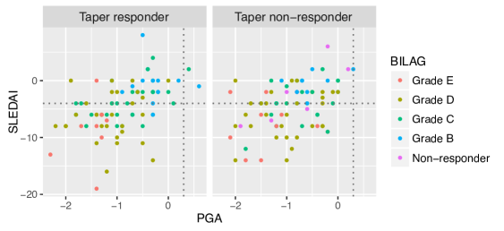
Figure 9: Observed response rates in each of the SLE responder index components in the Phase IIb MUSE trial. SLEDAI is plotted on the y-axis and PGA on the x-axis, along with their corresponding dichotomisation thresholds. Levels of BILAG are represented by different colours and taper responders and non-responders are split across two panels.

5.2 Results

The probability of response in the placebo arm is estimated as 0.199 by the latent variable method, 0.211 by the augmented binary method and 0.224 by the standard binary method. A much larger discrepancy between the methods is shown in the treatment arm, where the probability of response is estimated at 0.311, 0.324 and 0.382 in the latent variable, augmented binary and standard binary methods respectively.

The log-odds treatment effect point estimates and confidence intervals for the MUSE trial are shown in Table 4. Both joint modelling methods estimate the treatment effect more precisely. Although there may be bias present in the point estimates for the joint modelling methods, the confidence intervals entirely overlap with that of the binary method. All three methods indicate that anifrolumab 300mg performs better than placebo, as in the original findings. The latent variable model fits the data well according to the modified Pearson residuals, see Appendix G.

The simulation results indicated that the latent variable method may report the treatment effect with bias and have problems with bias related under-coverage when the treatment effect is large and when the assumption of joint normality is not satisfied. As the problems with the performance are bias related, we suggest implementing a bootstrap procedure to correct for this. In this scenario N=182 and $n_{boot}$=1000, therefore the procedure is as follows:

1. Sample with replacement N=182 patients from the MUSE trial

2. Compute the treatment effect using the latent variable, augmented binary and standard binary methods

3. Repeat step 1 and 2 $n_{boot}$=1000 times

4. Obtain an estimate of the bias using the difference between the treatment effect in the MUSE trial and the mean of the bootstrap treatment effects

A 95% bootstrap confidence interval for the treatment effect estimate can be obtained by ordering the 1000 bootstrap estimates of the treatment effect and taking the $25^{th}$ and $975^{th}$ estimate. The point estimates and 95% confidence intervals from the MUSE trial and from the bootstrap re-sampling are shown in Table 4.

Table 4: Log-odds treatment effect estimates and 95% confidence intervals from the latent variable method, augmented binary method and standard binary method in the Phase IIb MUSE trial and the bootstrap sample when N=182 and $n_{boot}=1000$

Method	Log-odds treatment effect
	MUSE trial estimate	Bootstrap estimate
Latent Variable	0.641 (0.217, 1.072)	0.682 (0.275, 1.137)
Augmented binary	0.580 (0.139, 1.021)	0.608 (0.096, 1.111)
Binary	0.763 (0.078, 1.449)	0.809 (0.112, 1.561)

The log-odds point estimate from the latent variable method has been shifted away from the null by approximately 0.04. This is the magnitude of bias that the simulation results suggested for this treatment effect. The width of the confidence interval hasn’t changed much from the original estimate in the bootstrap sample, indicating that the variance is well estimated in the trial dataset. The point estimate for the binary method has also been shifted substantially, despite the simulations showing this method to be unbiased. This is likely due to the large imprecision in the treatment effect reported by the binary method.

In terms of estimated precision, it is interesting to determine where the trial data set lies in the distribution of datasets generated in the simulation study. The latent variable method reports the treatment effect 2.5 times more precisely than the standard binary method in this setting, whilst the augmented binary method is 2.4 times more precise. We would have expected this similar performance as the augmented binary method models the SLEDAI and taper variables - the only components driving response. This increase in precision from the latent variable method compared with the binary method amounts to a 60% reduction in required sample size.

6 Discussion

In this paper we addressed the issue of substantial losses of information when modelling complex composite endpoints. By employing concepts of partitioning latent variable outcome spaces we could model the observed structure of the composite endpoint, which resulted in large gains in efficiency. Sensitivity analyses showed that a bias is introduced when the assumptions of joint normality were not satisfied, however similar reductions in variance were observed. When applying the methods to the MUSE trial, we implemented a bootstrap procedure to correct for the presumed bias, as joint normality could not be assessed. The treatment effect was reported 2.5 times more precisely than that reported from the standard binary method.
Bias correction appears to perform well in the real data, where the crucial assumptions cannot be tested. The point estimate is shifted by a magnitude that would have been expected from the simulation results and the estimate of the variance is similar to that obtained in the single trial dataset. Furthermore the bootstrap confidence interval for the treatment effect is contained within that for the binary method, which offers further reassurance for application. However, more work could be done to investigate different structures and scenarios to ensure that the bias correction is always performing as expected. Ideally, we would investigate this further across a large number of datasets however this is too computationally intensive. To perform this on one replicate, where $n_{boot}=1000$ using 200 cores on a high performance computer (HPC) currently takes 7 hours. Exploring this further through bootstrapping or employing alternative multivariate distributions is an area for future research.
The precision gains offered by the latent variable method offer justification for the additional complexity. However, the magnitude of these gains are highly dependent on the components that drive response. The baseline case in the simulations was chosen to reflect when a composite endpoint is recommended for use, i.e. when all four components determine response rates. In this scenario, the precision gains achieved resulted in the latent variable method reporting the effect 2.5 to 17.5 times more precisely than the standard binary method. However, in practice in SLE trials, this has not been found to be the case. A review of two phase 3 trials (N= 2262) using the SRI-5 index found the SRI-5 response rate at week 52 for all patients was 32.8% (Kalunian and others (2018)). Non-response due to a lack of SLEDAI improvement, concomitant medication non-compliance or dropout was 31, 16.5 and 19.1%, respectively. Non-response due to deterioration in BILAG or Physician’s Global Assessment after SLEDAI improvement, concomitant medication compliance and trial completion was 0.5%. This is in agreement with our findings from the MUSE trial data, which suggests that the precision gains in the baseline case are optimistic. The simulation results show that when one continuous and one binary component drive response, the latent variable method may be anywhere between 1 and 12 times as precise as the binary method and up to 7 times as precise as the augmented binary method. In a very small number of cases ($<$2%) there are no efficiency gains from using the latent variable method in this scenario. However the potential gains available in 98% of cases ensures that implementing the latent variable method is still very much a worthwhile endeavour, for all stakeholders in a clinical trial.
In addition to SLE, we have identified other disease areas that have a similar complex composite structure, meaning the potential to improve efficiency extends well beyond SLE. However, it must be acknowledged that the exact structure of the endpoint may offer different magnitudes of bias and precision, and may require longer computational time. Furthermore, in conditions where longitudinal data is required to sufficiently capture disease activity, trials may include multiple follow-up times and the method will need to be extended to include latent variables in the mean structure to account for this. In terms of scalability to more complex endpoints, the computational time depends on many things, in particular the number of outcomes, the outcome scale and the number of levels in the ordinal variable. In our case, we find the number of ordinal levels to be the most influential factor in computational time. This is due to the fact that 5 levels in the ordinal variable leads to 10 probability calculations in (6), however 3 levels would require the computation of 6 joint probabilities. Consequently, the run time will be substantially increased if there are multiple ordinal levels and decreased if the discrete variables are binary. If the computational time for a particular endpoint is deemed to be too large, then we may reduce the complexity of the endpoint by collapsing the least informative components in to a single binary variable. It must be acknowledged that as we have coded the likelihood, with no package available to do this, the likelihood and probability of response code will have to be tailored specifically to each endpoint. The potential gains in efficiency justify this additional complexity.
We have shown that the latent variable method is a powerful tool in composite endpoint analysis and should be considered as a primary analysis method in a trial using these endpoints. In order for implementation in the general case, where the composite contains any number of continuous and discrete outcomes and to ensure the uptake of the method in clinical trials, we will need to develop a software package. Furthermore, if patients and investigators are to benefit from the efficiency gains, we will need a method to calculate the required sample size in a given trial. We are currently working on addressing these issues to aid in the application of the method.

Supplementary material

Appendix A

The joint probability below expresses, for patient i with $Y_{1}=y_{i1}$ and $Y_{2}=y_{i2}$, the probability that they will have a $Y_{3}$ score $w$ and a $Y_{4}$ score $k$.

$$pr\left(Y_{i3}=w,Y_{i4}=k|Y_{i1}=Y_{i1},y_{i2}=y_{i2};\boldsymbol{\theta}\right)=\\ \Phi_{2}\left(\tau_{w3}-\mu_{3|1,2},\tau_{k4}-\mu_{4|1,2};\Sigma_{3,4|1,2}\right)-\Phi_{2}\left(\tau_{(w-1)3}-\mu_{3|1,2},\tau_{k4}-\mu_{4|1,2};\Sigma_{3,4|1,2}\right)-\\ \Phi_{2}\left(\tau_{w3}-\mu_{3|1,2},\tau_{(k-1)4}-\mu_{4|1,2};\Sigma_{3,4|1,2}\right)+\Phi_{2}\left(\tau_{(w-1)3}-\mu_{3|1,2},\tau_{(k-1)4}-\mu_{4|1,2};\Sigma_{3,4|1,2}\right)$$ (10)

The intuition for the joint probability can be seen below in Figure 10, specifically for the SLE endpoint, where $w=5$ and $k=2$.

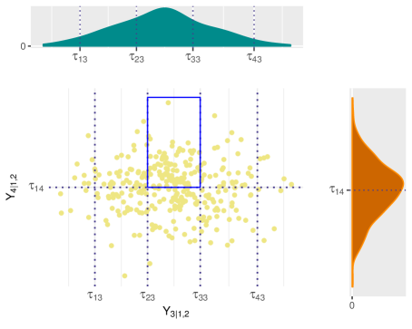
Figure 10: The figure shows the conditional outcome $Y_{3|1,2}$ on the x-axis and $Y_{4|1,2}$ on the y-axis with their corresponding underlying continuous densities and partitioning thresholds. The area where $w=3$ and $k=2$ is highlighted for illustration

The blue box indicates the region where $w=3$ and $k=2$. As $\tau_{03}=\tau_{04}=-\infty$ and $\tau_{53}=\tau_{24}=\infty$, the corresponding probability is shown in (11).

$$pr\left(Y_{i3}=3,Y_{i4}=2|Y_{i1}=y_{i1},Y_{i2}=y_{i2};\boldsymbol{\theta}\right)=\\ \Phi_{2}\left(\tau_{33}-\mu_{3|1,2},\infty-\mu_{4|1,2};\Sigma_{3,4|1,2}\right)-\Phi_{2}\left(\tau_{23}-\mu_{3|1,2},\infty-\mu_{4|1,2};\Sigma_{3,4|1,2}\right)-\\ \Phi_{2}\left(\tau_{33}-\mu_{3|1,2},\tau_{(14}-\mu_{4|1,2};\Sigma_{3,4|1,2}\right)+\Phi_{2}\left(\tau_{23}-\mu_{3|1,2},\tau_{14}-\mu_{4|1,2};\Sigma_{3,4|1,2}\right)$$ (11)

Appendix B

One suggestion in the literature for assessing goodness-of-fit in latent variable models is introduced by Samani and Ganjali (2008) for the case when there is one continuous and one ordinal variable. This may be extended to allow for two continuous, one ordinal and one binary outcome for application in SLE, as shown below.
As before, let $\mathbf{Y}_{i}=(Y_{i1},Y_{i2},Y_{i3},Y_{i4})^{\prime}$ be the vector of observed responses for patient i. Then, partitioning the observed and latent continuous measures, we let $\mathbf{Y_{cts}}=(Y_{1},Y_{2})$ and $\mathbf{Y_{dis}}=(Y_{3},Y_{4})$. Then, $\hat{\Sigma}_{11}=\hat{Var}(\mathbf{Y_{cts}}),\hat{\Sigma}_{22}=\hat{Var}(\mathbf{Y_{dis}}),\hat{\Sigma}_{12}=\hat{\Sigma}_{21}=\hat{Cov}(\mathbf{Y_{cts}},\mathbf{Y_{dis}})$.
The modified Pearson residuals, taking in to account the correlation between responses are shown below.

$$r_{i}^{p}=\hat{\Sigma}^{-\frac{1}{2}}(Y_{i}-\hat{\mu_{i}})$$ (B.1)

where,

$$\boldsymbol{\hat{\mu_{i}}}=(\hat{E}(Y_{i1},Y_{i2}\mid X_{i1},X_{i2}),\hat{E}(Y_{i3},Y_{i4}\mid X_{i3},X_{i4}))^{\prime}$$ (B.2)

and

$$\hat{\Sigma}=\begin{pmatrix}\hat{\Sigma}_{11}&\hat{\Sigma}_{12}\\ \hat{\Sigma}_{21}&\hat{\Sigma}_{22}\\ \end{pmatrix}$$ (B.3)

A Cholesky decomposition may be used to obtain $\hat{\Sigma}^{-\frac{1}{2}}$ in (B.1). The covariance between the vector of observed continuous and observed discrete responses is shown below.

$$\Sigma_{12}= E(\mathbf{Y_{cts}Y_{dis}})-E(\mathbf{Y_{cts}})E(\mathbf{Y_{dis}})$$

$$= E(\mathbf{Y_{cts}}E(\mathbf{Y_{dis}}\mid\mathbf{Y_{cts}}))-E(\mathbf{Y_{cts}})E(\mathbf{Y_{dis}})$$

$$= E(Y_{1}Y_{2}E(Y_{3},Y_{4}\mid Y_{1},Y_{2}))-E(\mathbf{Y_{cts}})E(\mathbf{Y_{dis}})$$

$$= \int_{y_{1}}\int_{y_{2}}y_{1}y_{2}\sum_{y_{3}}\sum_{y_{4}}y_{3}y_{4}P\left(Y_{3}=w,Y_{4}=k|Y_{1}=y_{1},Y_{2}=y_{2}\right)f_{Y_{1},Y_{2}}(y_{1},y_{2})dy_{1}dy_{2}$$

$$\hskip 264.61063pt-E(\mathbf{Y_{cts}})E(\mathbf{Y_{dis}})$$

Where,

$$P\left(Y_{3}=w,Y_{4}=k|Y_{1}=y_{1},Y_{2}=y_{2}\right)=\\ \Phi\left(\tau_{w3}-\mu_{3|1,2},\tau_{k4}-\mu_{4|1,2};\Sigma_{3,4|1,2}\right)-\Phi\left(\tau_{(w-1)3}-\mu_{3|1,2},\tau_{k4}-\mu_{4|1,2};\Sigma_{3,4|1,2}\right)-\\ \Phi\left(\tau_{w3}-\mu_{3|1,2},\tau_{(k-1)4}-\mu_{4|1,2};\Sigma_{3,4|1,2}\right)+\Phi\left(\tau_{(w-1)3}-\mu_{3|1,2},\tau_{(k-1)4}-\mu_{4|1,2};\Sigma_{3,4|1,2}\right)$$

$$E(\mathbf{Y_{cts}})=\int_{y_{1}}\int_{y_{2}}y_{1}y_{2}f_{Y_{1},Y_{2}}(y_{1},y_{2})dy_{1}dy_{2}$$

$$E(\mathbf{Y_{dis}})=\sum_{y_{3}}\sum_{y_{4}}y_{3}y_{4}P\left(Y_{3}=w,Y_{4}=k\right)$$

and

$$P(Y_{3}=w,Y_{4}=k)=\Phi( \tau_{w3}-\mu_{3},\tau_{k4}-\mu_{4};\rho_{3,4})-\Phi(\tau_{(w-1)3}-\mu_{3},\tau_{k4}-\mu_{4};\rho_{3,4})-$$

$$\Phi( \tau_{w3}-\mu_{3},\tau_{(k-1)4}-\mu_{4};\rho_{3,4})+\Phi(\tau_{(w-1)3}-\mu_{3},\tau_{(k-1)4}-\mu_{4};\rho_{3,4})$$

The Pearson residual is based on the Pearson goodness-of-fit statistics

$$\chi_{p}^{2}=\sum_{i=1}^{n}\chi_{p}^{2}(Y_{i},\hat{\mu_{i}})$$ (B.4)

with ith component

$$\chi_{p}^{2}(Y_{i},\hat{\mu_{i}})=(Y_{i}-\hat{\mu_{i}})^{\prime}\hat{\Sigma}^{-1}(Y_{i}-\hat{\mu_{i}})$$ (B.5)

The distribution of the residuals should follow a chi-squared distribution with p degrees of freedom. Comparing the residuals to the chi-squared value allows us to identify observations which the model does not fit well. If there are many observations unexplained by the model then it could indicate a poor choice of model. This may be due to the covariance structure $\hat{\Sigma}$ and its assumed distribution. The model may be refitted with various covariance structures and to obtain a model which is found to satisfactorily explain the observed data. If this is not achieved then joint normality of the error terms may be an unreasonable assumption indicating that the latent variable model may not be appropriate. It is possible to fit latent variable models which assume a different multivariate distribution for the error terms, however this is not considered here.

Appendix C

Augmented binary method

The augmented binary model is shown below. The baseline measures for $Y_{i1}$ and $Y_{i2}$ are included for comparison, as they are accounted for in the mean structure of the latent variable method. As one time point is modelled we can use a linear model for $Y_{i1}$ as shown in (C.1). Note that $Y_{i1}$ or $Y_{i2}$ may be chosen as the continuous measure to retain and should always be determined by which is the most informative.

$$Y_{i1}=\delta_{0}+\delta_{1}T{i}+\delta_{2}y_{i10}+\delta_{3}y_{i20}+\varepsilon_{i}$$ (C.1)

where $\varepsilon_{i}|T_{i},y_{i10},y_{i20}\sim N(0,\sigma)$. In this case, the failure time binary indicator will contain information from the remaining three components. $F_{i}$ is set to equal 0 if $Y_{i2}\leq\theta_{2},Y_{i3}$ is Grade B-E and $Y_{i4}=0$, otherwise the patient is labelled a non-responder in these components and $F_{i1}=1$. $F_{i}$ is modelled using the logistic regression model in (C.2).

$$logit(Pr(F_{i}=1|T_{i},y_{i10},y_{i20})=\alpha_{F}+\beta_{F}T_{i}+\gamma_{F}y_{i10}+\psi_{F}y_{i20}$$ (C.2)

Maximum likelihood estimates for the parameters are obtained from fitting models (C.1) and (C.2). The probability of response is shown in (C.3).

$$P(Y_{i1}\leqslant\theta_{1},F_{i1}=0|T_{i},y_{i10},y_{i20})\\ =\int_{-\infty}^{\theta_{1}}P(F_{i1}=0|T_{i},y_{i10},y_{i20})f_{Y_{1}}(y_{i1};T_{i},y_{i10},y_{i20})dy_{i1}$$ (C.3)

As in the latent variable method, (C.3) is used to obtain probability of response estimates for each patient, assuming they were treated $\tilde{p_{i1}}$ and not treated $\tilde{p_{i1}}$, which are used to define an odds ratio, risk ratio or risk difference.

Standard binary method

The standard binary method is a logistic regression on the overall responder index, as shown in (C.4).

$$logit(Pr(S_{i}=1|T_{i},y_{i10})=\alpha+\beta T_{i}+\gamma y_{i10}+\psi y_{i20}$$ (C.4)

The odds ratio and standard error estimates can be obtained directly.

Appendix D

Table 5: Performance measures and Monte Carlo standard errors used to assess the behaviour of the latent variable, augmented binary and binary methods in a simulation study for the systemic lupus erythematosus composite endpoint

Performance measure	Estimate	MCSE
Bias	$\frac{1}{n_{sim}}\sum\limits_{j=1}^{n_{sim}}\hat{\theta}_{j}-\theta$	$\sqrt{\frac{1}{n_{sim}(n_{sim}-1)}\sum\limits_{j=1}^{n_{sim}}(\hat{\theta}_{j}-\bar{\theta})^{2}}$
Coverage	$\frac{1}{n_{sim}}\sum\limits_{j=1}^{n_{sim}}1(\hat{\theta}_{low,j}\leq\theta\leq\hat{\theta}_{upp,j})$	$\sqrt{\frac{\hat{cov.}(1-\hat{cov.})}{n_{sim}}}$
Bias-corrected coverage	$\frac{1}{n_{sim}}\sum\limits_{j=1}^{n_{sim}}1(\hat{\theta}_{low,j}\leq\bar{\theta}\leq\hat{\theta}_{upp,j})$	$\sqrt{\frac{\hat{BEcov.}(1-\hat{BEcov.})}{n_{sim}}}$
Power	$\frac{1}{n_{sim}}\sum\limits_{j=1}^{n_{sim}}1(p_{j}<\alpha)$	$\sqrt{\frac{\hat{Power}(1-\hat{Power})}{n_{sim}}}$
MSE	$\sum\limits_{j=1}^{n_{sim}}(\hat{\theta}_{j}-\theta)^{2}$	$\sqrt{\frac{\sum\limits_{j=1}^{n_{sim}}[(\hat{\theta}_{j}-\theta)^{2}-\hat{MSE}]^{2}}{n_{sim}(n_{sim}-1)}}$
Empirical SE	$\sqrt{\frac{1}{n_{sim}-1}\sum\limits_{j=1}^{n_{sim}}(\hat{\theta}_{i}-\bar{\theta})^{2}}$	$\frac{\hat{EmpSE}}{\sqrt{2(n_{sim}-1)}}$
Model SE	$\sqrt{\frac{1}{n_{sim}-1}\sum\limits_{j=1}^{n_{sim}}\hat{Var}(\hat{\theta}_{j})}$	$\sqrt{\frac{\hat{Var}[\hat{Var}(\hat{\theta})]}{4n_{sim}\hat{ModSE}^{2}}}\dagger$
Relative precision A vs. B	$\frac{\hat{Var}(\hat{\theta}_{j})_{B}}{\hat{Var}(\hat{\theta}_{j})_{A}}$	-

• $\hat{\theta}_{j}:$ estimated log-odds treatment effect in simulated data j

• $\bar{\theta}$: mean log-odds treatment effect over $n_{sim}$ datasets

• $\hat{\theta}_{low,j},\hat{\theta}_{upp,j}$ lower and upper limit of confidence interval for iteration j

• $\hat{Var}[\hat{Var}(\hat{\theta})]=\frac{1}{n_{sim}-1}\sum_{j=1}^{n_{sim}}\{\hat{Var}(\hat{\theta}_{i})-\frac{1}{n_{sim}}\sum_{j=1}^{n_{sim}}\hat{Var}(\hat{\theta}_{j})\}^{2}$

Appendix E

Table 6: Parameter values for the simulated scenarios which investigate the effect of varying responder threshold $\theta_{1}$, changing the components driving response and differing treatment effects on the performance of the latent variable, augmented binary and standard binary methods for the systemic lupus erythematosus composite endpoint

Scenario	Parameters	Investigates
$\theta_{1}=-2$	$\theta_{1}=-2$	100% of patients respond in $Y_{1}$
$\theta_{1}=-3$	$\theta_{1}=-3$	96% of patients respond in $Y_{1}$
$\theta_{1}=-4$	$\theta_{1}=-4$	82% of patients respond in $Y_{1}$
$\theta_{1}=-5$	$\theta_{1}=-5$	52% of patients respond in $Y_{1}$
$\theta_{1}=-6$	$\theta_{1}=-6$	20% patients respond in $Y_{1}$
$Y_{1},Y_{4}$	$\theta_{1}=-5,\theta_{2}=2,\theta_{3}=2$	Continuous and binary variable driving response
$Y_{4}$	$\theta_{1}=-2,\theta_{2}=2,\theta_{3}=2$	Binary variable driving response
$Y_{1},Y_{2},Y_{3}$	$\theta_{4}=2$	Two continuous and ordinal drive response
Treat case 1	$\alpha_{0}=-4.9,\alpha_{1}=-0.09,\beta_{0}=-1.2,$ $\beta_{1}=-0.11,\gamma_{1}=-0.145,\psi_{0}=-0.2,$ $\psi_{1}=-0.07$	Odds ratio = 1.217
Treat case 2	$\alpha_{0}=-4.9,\alpha_{1}=-0.20,\beta_{0}=-1.2,$ $\beta_{1}=-0.25,\gamma_{1}=-0.2,\psi_{0}=-0.2,$ $\psi_{1}=-0.12$	Odds ratio = 1.426
Treat case 3	$\alpha_{0}=-4.9,\alpha_{1}=-0.30,\beta_{0}=-1.2,$ $\beta_{1}=-0.50,\gamma_{1}=-0.3,\psi_{0}=-0.2,$ $\psi_{1}=-0.22$	Odds ratio = 1.794
Treat case 4	$\alpha_{0}=-4.9,\alpha_{1}=-0.32,\beta_{0}=-1.2,$ $\beta_{1}=-0.65,\gamma_{1}=-0.39,\psi_{0}=-0.2,$ $\psi_{1}=-0.27$	Odds ratio = 2.007
Treat case 5	$\alpha_{0}=-4.9,\alpha_{1}=-0.33,\beta_{0}=-1.2,$ $\beta_{1}=-0.72,\gamma_{1}=-0.45,\psi_{0}=-0.2,$ $\psi_{1}=-0.33$	Odds ratio = 2.198

Appendix F

Multivariate skew-normal distribution

To test the robustness of the latent variable method to deviations from joint normality of the components, we can generate the data so that the components are drawn from a multivariate skew-normal. The multivariate skew-normal is an extension of the univariate skew-normal distribution introduced by multskew. They define it as follows. A random vector Y=$(Y_{1},...,_{k})^{T}$ has k-variate skew-normal distribution, if its density function is

$$f_{k}(\mathbf{y})=2\phi_{k}(\mathbf{y;\Omega})\Phi(\boldsymbol{\alpha}^{T}\mathbf{y}),\mathbf{y}\in\mathbf{R}^{k}$$ (F.1)

where $\phi_{k}(\mathbf{y;\Omega})$ is the probability density function of the k-variate normal distribution with standardised marginals and correlation matrix $\mathbf{\Omega}$. The shape parameter $\boldsymbol{\alpha}$ determines the skewness, where $\boldsymbol{\alpha}=\mathbf{0}$ reduces the density in (F.1) to the N($\mathbf{0},\boldsymbol{\Omega}$) density.
Scenarios of interest are shown in Table 7. The first scenario considers when all four components are skewed. Scenarios 2-3 consider different magnitudes of skew in the latent continuous components only. This tests the robustness of the method to the assumption that the observed discrete variables manifest from continuous variables. Scenario 4 is the null case for scenario 3.

Table 7: Simulation scenarios considered to investigate deviations from joint normality for the components of the systemic lupus erythematosus composite endpoint based on the multivariate skew-normal distribution where $\boldsymbol{\alpha}$ determines the magnitude of the skew in each component

Scenario	$\boldsymbol{\alpha}$	Purpose
skew1	(0.1, 0.1, 0.1, 0.1)	Skew in all four components
skew2	(0, 0, 0.1, 0.1)	Skew in discrete components only
skew3	(0, 0, 0.05, 0.05)	Smaller skew in discrete components only
skew4	(0, 0, 0.05, 0.05)	Smaller skew in discrete components only in the null case

Results

The bias, coverage, bias-corrected coverage and power are shown in Table 8 for all four scenarios. In scenarios 1-3, the non-normality introduces bias which results under-coverage. The bias-corrected coverage is close to nominal for all scenarios however the coverage of the latent variable method is nominal in the null case. This is consistent with our findings when the joint normality assumption is satisfied in that bias is introduced in the estimation of the treatment arm, however the magnitude of this bias is much smaller when the assumptions are satisfied. The augmented binary and standard binary methods behave similarly to when the joint normality assumptions are satisfied, which is expected given that the assumptions of those models are violated in both contexts. The latent variable method still offers large power gains over the other methods.

Table 8: Operating characteristics of the latent variable, augmented binary and binary methods when the components of the systemic lupus erythematosus endpoint are drawn from a multivariate skew-normal, N=300 and $n_{sim}=1000$

Performance measure	Scenario	Method
		Latent Variable	Augmented Binary	Binary
Bias	skew1	-0.173 (0.012)	0.041 (0.252)	-0.015 (0.258)
	skew2	-0.103 (0.008)	0.036 (0.251)	-0.020 (0.255)
	skew3	-0.068 (0.008)	0.038 (0.244)	-0.016 (0.245)
	skew4	-0.033 (0.008)	0.007 (0.254)	0.001 (0.255)
Coverage	skew1	0.556 (0.018)	0.933 (0.009)	0.939 (0.009)
	skew2	0.811 (0.013)	0.928 (0.008)	0.941 (0.008)
	skew3	0.884 (0.010)	0.934 (0.008)	0.950 (0.007)
	skew4	0.933 (0.009)	0.923 (0.009)	0.950 (0.008)
Bias-corrected	skew1	0.962 (0.007)	0.929 (0.009)	0.943 (0.008)
coverage	skew2	0.936 (0.008)	0.930 (0.008)	0.943 (0.007)
	skew3	0.940 (0.008)	0.929 (0.008)	0.954 (0.007)
	skew4	0.948 (0.008)	0.926 (0.009)	0.950 (0.008)
Power	skew1	0.897 (0.011)	0.646 (0.017)	0.487 (0.018)
	skew2	0.959 (0.006)	0.637 (0.015)	0.471 (0.016)
	skew3	0.982 (0.004)	0.641 (0.015)	0.495 (0.016)
	skew4	-	-	-

Table 9 shows the MSE, empirical SE and model SE of the three methods. The latent variable method performs best consistently across these performance measures. The augmented binary and standard binary methods have an MSE across all scenarios of approximately 0.06 whilst the MSE of the latent variable method is between 0.01 and 0.04. This indicates that the large reduction in variance is useful despite the introduction of bias. We acknowledge however that this may not hold across all sample sizes (Morris and others (2017)).

Table 9: Operating characteristics (Monte Carlo standard errors in parentheses) of the latent variable, augmented binary and binary methods when the components of the systemic lupus erythematosus endpoint are drawn from a multivariate skew-normal, N=300 and $n_{sim}=1000$

Performance measure	Scenario	Method
		Latent Variable	Augmented Binary	Binary
MSE	skew1	0.039 (0.001)	0.063 (0.003)	0.066 (0.003)
	skew2	0.021 (0.001)	0.063 (0.003)	0.065 (0.003)
	skew3	0.014 (0.001)	0.060 (0.003)	0.060 (0.003)
	skew4	0.010 (0.001)	0.064 (0.004)	0.065 (0.003)
EmpSE	skew1	0.097 (0.003)	0.248 (0.006)	0.257 (0.007)
	skew2	0.102 (0.002)	0.249 (0.006)	0.254 (0.006)
	skew3	0.099 (0.002)	0.241 (0.005)	0.245 (0.006)
	skew4	0.094 (0.002)	0.254 (0.006)	0.255 (0.006)
ModSE	skew1	0.010 (0.006)	0.052 (0.001)	0.064 (0.001)
	skew2	0.010 (0.003)	0.050 (0.001)	0.060 (0.001)
	skew3	0.010 (0.015)	0.048 (0.001)	0.059 (0.001)
	skew4	0.009 (0.004)	0.051 (0.001)	0.063 (0.001)

Table 10 shows the probability of response in each arm for each of the methods. The findings are consistent with when the assumptions are satisfied. Namely, the latent variable method estimates the probability of response in the control arm well however underestimates the probability of response in the treatment arm. The magnitude of this underestimation is unaffected by the degree of skew or whether the skew is present in the observed continuous components.

Table 10: Estimated probability of response in the treatment and placebo arms from the latent variable model (Lat Var), augmented binary method (Aug Bin) and standard binary method (Bin) when the components of the systemic lupus erythematosus endpoint are drawn from a multivariate skew-normal, N=300 and $n_{sim}=1000$

	$Pr(resp\mid T=0)$				$Pr(resp\mid T=1)$
Scenario	True	Lat Var	Aug Bin	Bin	True	Lat Var	Aug Bin	Bin
skew1	0.259	0.263	0.221	0.258	0.365	0.330	0.326	0.359
skew2	0.290	0.287	0.253	0.290	0.398	0.370	0.361	0.392
skew3	0.309	0.302	0.271	0.308	0.418	0.394	0.382	0.413
skew4	0.309	0.299	0.269	0.307	0.309	0.292	0.270	0.307

The odds ratio treatment effect estimate from each method is shown in Table 11. The latent variable method is biased towards the null, the augmented binary method is biased away from the null. The binary method slightly underestimates the treatment effect in this setting however all are close to true for the null case.

Table 11: Estimated odds ratio treatment effect from the latent variable model (Lat Var), augmented binary method (Aug Bin) and standard binary method (Bin) when the components of the systemic lupus erythematosus endpoint are drawn from a multivariate skew-normal, N=300 and $n_{sim}=1000$

	Treatment effect
Scenario	True	Lat Var	Aug Bin	Bin
skew1	1.640	1.379 (1.140, 1.668)	1.708 (1.093, 2.668)	1.616 (0.985, 2.651)
skew2	1.617	1.459 (1.203, 1.770)	1.676 (1.083, 2.594)	1.586 (0.980, 2.565)
skew3	1.611	1.505 (1.243, 1.822)	1.674 (1.089, 2.572)	1.585 (0.987, 2.548)
skew4	1.000	0.967 (0.807, 1.160)	1.007 (0.647, 1.566)	1.001 (0.613, 1.634)

The median relative precision of the methods are shown in Table 12, with the 10th centile and 90th centile values. These are consistent with our previous findings indicating that the violation of joint normality only affects the bias and not the variance.

Table 12: Estimated relative precision from the latent variable model (Lat Var), augmented binary method (Aug Bin) and standard binary method (Bin) when the components of the systemic lupus erythematosus endpoint are drawn from a multivariate skew-normal, N=300 and $n_{sim}=1000$

	Treatment effect
Scenario	Lat Var vs Bin	Lat Var vs Aug Bin	Aug Bin vs Bin
skew1	6.903 [5.336, 8.972]	5.579 [4.376, 7.313]	1.231 [1.189, 1.275]
skew2	6.263 [5.013, 7.917]	5.177 [4.096, 6.518]	1.213 [1.178, 1.252]
skew3	6.326 [5.016, 7.995]	5.192 [4.098, 6.548]	1.219 [1.184, 1.257]
skew4	7.384 [5.729, 9.343]	5.985 [4.655, 7.629]	1.231 [1.192, 1.273]

Appendix G

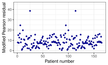
Figure 11: Plot of the modified Pearson residuals from the latent variable model for each patient in the MUSE trial. The residuals highlight that two patients observations are poorly explained by the model but that the model is a good fit for the remaining patients.

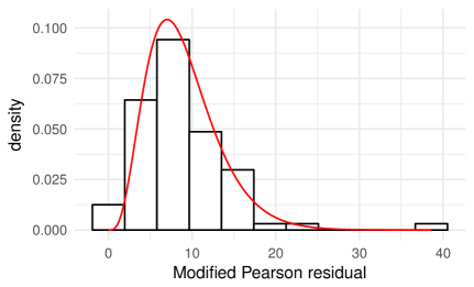
Figure 12: Histogram of the modified Pearson residuals from the latent variable model in the MUSE trial dataset with the corresponding $\chi^{2}$ density. The modified Pearson residuals should follow the distribution of the $\chi^{2}$ density shown if the model fits well.

References

- Arminger and Kusters (1988) Arminger, G. and Kusters, U. (1988). Latent trait and latent class models, Chapter Latent trait models with indicators of mixed measurement level. Plenum, pp. 51–73.
- Arnold (2009) Arnold, B.C. (2009). Flexible univariate and multivariate models based on hidden truncation. Journal of Statistical Planning and Inference 139, 3741–3749.
- Ashford and Sowden (1970) Ashford, J.R. and Sowden, R.R. (1970). Multivariate probit analysis. Biometrics 26, 535–46.
- Catalano (1997) Catalano, P.J. (1997). Bivariate modelling of clustered continuous and ordered categorical outcomes. Statistics in Medicine 16, 883–900.
- Catalano and Ryan (1992) Catalano, P.J. and Ryan, L.M. (1992). Bivariate latent variable models for clustered discrete and continuous outcomes. Journal of the American Statistical Association 87(419), 651–658.
- Chib and Greenberg (1998) Chib, Siddhartha and Greenberg, Edward. (1998). Analysis of multivariate probit models. Biometrika 85(2), 347–361.
- Cox and Wermuth (1992) Cox, D.R. and Wermuth, N. (1992). Response models for mixed binary and quantitative variables. Biometrika 79(3), 441–61.
- de Leon and Carriere (2013) de Leon, A.R. and Carriere, K.C. (editors). (2013). Analysis of Mixed Data Methods and Applications. Chapman and Hall/CRC.
- de Leon and Wu (2010) de Leon, A.R and Wu, B. (2010). Copula based regression models for a bivariate mixed discrete and continuous outcome. Statistics in Medicine 30, 175–185.
- Dunson (2000) Dunson, D.B. (2000). Bayesian latent variable models for clustered mixed outcomes. Journal of the Royal Statistical Society: Series B (Statistical Methodology) 62(2), 355–366.
- Faes and others (2002) Faes, C., Geys, H., Aerts, M., Catalano, P.J. and Molenberghs, G. (2002). Modelling combined continuous and ordinal outcomes from developmental toxicity studies. In: Stasinopoulos, M. and Touloumi, G. (editors), In Proceedings of the 17th International Workshop on Statistical Modelling. Chania, Crete.
- Fitzmaurice and Laird (1995) Fitzmaurice, G.M. and Laird, N.M. (1995). Regression models for a bivariate discrete and continuous outcome with clustering. Journal of the American Statistical Association 90, 845–852.
- Furie and others (2017) Furie, R., Khamashta, M., Merrill, J.T., Werth, V.P., Kalunian, K., Brohawn, P., Illei, G. G., Drappa, J., Wang, L., Yoo, S. and others. (2017). Anifrolumab, an anti interferon alpha receptor monoclonal antibody, in moderate-to-severe systemic lupus erythematosus. Arthritis and Rheumatology 69(2), 376–386.
- Genz (1992) Genz, A. (1992). Numerical computation of multivariate normal probabilities. Journal of Computational and Graphical Statistics 1, 141–150.
- Gueorguieva and Agresti (2001) Gueorguieva, R.V. and Agresti, A. (2001). A correlated probit model for joint modeling of clustered binary and continuous responses. Journal of the American Statistical Association 96(455), 1102–1112.
- Gueorguieva and Sanacora (2003) Gueorguieva, R.V. and Sanacora, G. (2003). A latent variable model for joint analysis of repeatedly measured ordinal and continuous outcomes. In: Verbeke, G., Molenberghs, G., Aerts, M. and Fiews, S. (editors), In Proceedings of the 18th International Workshop on Statistical Modelling. Katholieke Universiteit Leuven: Leuven. pp. 171–176.
- Gueorguieva and Sanacora (2006) Gueorguieva, R.V. and Sanacora, G. (2006). Joint analysis of repeatedly observed continuous and ordinal measures of disease severity. Statistics in Medicine.
- Kalunian and others (2018) Kalunian, Kenneth C, Urowitz, Murray B, Isenberg, David, Merrill, Joan T, Petri, Michelle, Furie, Richard A, Morgan-Cox, Mary-Ann, Taha, Rebecca, Watts, Steven, Silk, Maria and others. (2018). Clinical trial parameters that influence outcomes in lupus trials that use the systemic lupus erythematosus responder index. Rheumatology 57(1), 125–133.
- Lauritzen and Wermuth (1989) Lauritzen, S.L. and Wermuth, N. (1989). Graphical models for association between variables, some of which are qualitative and some quantitative. Annals of Statistics 17, 31–54.
- Lessafre and Molenberghs (1991) Lessafre, E. and Molenberghs, G. (1991). Multivariate probit analysis: A neglected procedure in medical statistics. Statistics in Medicine 10(9), 1391–1403.
- McCulloch (2008) McCulloch, C. (2008). Joint modelling of mixed outcome types using latent variables. Statistical Methods in Medical Research 17, 53–73.
- McMenamin and others (2018) McMenamin, M., A., Berglind and Wason, J.M.S. (2018). Improving the analysis of composite endpoints in rare disease trials. Orphanet Journal of Rare Diseases 13, 81.
- Morris and others (2017) Morris, T.P., White, I.R. and Crowther, M.J. (2017). Using simulation studies to evaluate statistical methods. arXiv:1712.03198.
- Nelsen (1999) Nelsen, R.B. (1999). An Introduction to Copulas: Definitions and Basic Properties. New York, NY: Springer New York.
- Olkin and Tate (1961) Olkin, I. and Tate, R.F. (1961). Multivariate correction models with mixed discrete and continuous variables. Annals of Mathematical Statistics 32, 448–465.
- Pearson (1904) Pearson, K. (1904). Mathematical contributions to the theory of evolution. xii. on a generalised theory of alternative inheritance, with special reference to mendel’s laws. Philosophical Transactions of the Royal Society of London. Series A, Containing Papers of a Mathematical or Physical Character 203, 53–86.
- Poon and Lee (1987) Poon, W.Y. and Lee, S.Y. (1987). Maximum likelihood estimation of multivariate polyserial and polychoric correlation coefficients. Psychometrika 52(3), 409–430.
- Regan and Catalano (2000) Regan, M.M. and Catalano, P.J. (2000). Regression models and risk estimation for mixed discrete and continuous outcomes in developmental toxicology. Risk Analysis 20, 363–376.
- Samani and Ganjali (2008) Samani, E.B. and Ganjali, M. (2008). A multivariate latent variable model for mixed continuous and ordinal responses. World Applied Sciences Journal 3(2), 294–299.
- Sammel and Ryan (2002) Sammel, M.D. and Ryan, L.M. (2002). Effects of covariance misspecification in a latent variable model for multiple outcomes. Statistica Sinica 12, 1207–1222.
- Sammel and others (1997) Sammel, M.D., Ryan, L.M. and Leger, J.M. (1997). Latent variable models for mixed discrete and continuous outcomes. J. R. Statist. Soc. B 59(3), 667–678.
- Skrondal and Rabe-Hesketh (2004) Skrondal, A. and Rabe-Hesketh, S. (2004). Generalized Latent Variable Modeling: Multilevel, Longitudinal and Structural Equation Models. Chapman and Hall/CRC.
- Tate (1955) Tate, R.F. (1955). The theory of correlation between two continuous variables when one is dichotomised. Biometrika 42(1-2), 205–216.
- Verbeke and others (2014) Verbeke, G., Fieuws, S. and Molenberghs, G. (2014). The analysis of multivariate longitudinal data: A review. Statistical Methods in Medical Research 23(1), 42–59.
- Wason and Jenkins (2016) Wason, J. and Jenkins, M. (2016). Improving the power of clinical trials of rheumatoid arthritis by using data on continuous scales when analysing response rates: an application of the augmented binary method. Rheumatology 55(10), 1796–1802.
- Wason and Seaman (2013) Wason, J. and Seaman, S. R. (2013). Using continuous data on tumour measurements to improve inference in phase ii cancer studies. Statistics in Medicine 32(26), 4639–4650.
- Whittaker (1990) Whittaker, J. (1990). Graphical Models in Applied Multivariate Statistics. Wiley and Sons.
- Wu and de Leon. A.R. (2014) Wu, B. and de Leon. A.R. (2014). Gaussian copula mixed models for clustered mixed outcomes, with application in developmental toxicology. JABES 19(1), 39–56.