Spatial modulation of the electromagnetic energy transfer by excitation of graphene waveguide surface plasmons

Abstract

We theoretically study the electromagnetic energy transfer between donor and acceptor molecules near a graphene waveguide. The surface plasmons (SPs) supported by the structure provide decay channels which lead to an improvement in the energy transfer rate when the donor and acceptor are localized on the same side or even on opposite sides of the waveguide. The modification of the energy transfer rate compared to its value in absence of the waveguide are calculated by deforming the integration path into a suitable path in the complex plane. Our results show that this modification is dramatically enhanced when the symmetric and antisymmetric SPs are excited. Notable effects on the spatial dependence of the energy transfer due to the coherent interference between these SP channels, which can be tuned by chemical potential variations, are highlighted and discussed in terms of SP propagation characteristics.

Keywords: Electromagnetic energy transfer, graphene, surface plasmons

1 Introduction

The electromagnetic resonance energy transfer (RET) between pairs of quantum emitters, such as atoms, molecules or quantum dots, can be largely altered by excitation of electromagnetic eigenmodes. By coupling these emitters to a designed wave guiding or surface plasmon (SP) mode environments, a significant directional control and RET enhancement has been achieved [1, 2, 3, 4, 5, 6] allowing energy transfer over distances larger than the Förster energy transfer range [7]. New avenues have emerged with the advent of graphene, a monolayer of carbon atoms arranged in a hexagonal lattice, which has motivated an extensive wealth of theoretical analysis concerning the shift of molecular interplay control via metal SPs, currently working in the visible range, to the mid–infrarred and terahertz frequencies [8, 9, 10].

Key representatives of SPs on doped graphene are those with $p$ polarization, existing below a critical frequency depending of the chemical potential on graphene, which offer high confinement, relatively low loss and good tunability of its spectrum through electrical or chemical modification of the carrier density [11, 12].

Because of their fundamental properties as well as their potential applications, the knowledge about the interaction between graphene and electromagnetic radiation via SP mechanism is a topic of continuously increasing interest, opening the route towards a wide spectrum of studies ranging from photonic devices capable to achieve invisibility [13, 14] and THz antennas [15, 16, 17, 18] to graphene SP structures capable to control the spontaneous emission as well as the RET between quantum emitters [19, 20, 21, 22, 23, 24, 25].

In this paper we study the energy transfer process between a donor and acceptor placed in close proximity to a waveguide formed by two parallel graphene sheets with an insulator spacer layer. Particular interest is paid to the role of the SPs of the structure in modifying the energy transfer rate with respect to the rate in absence of the waveguide. This issue has been addressed for a single graphene sheet [19, 26, 27], where the main results have shown a broadband and long–range energy transfer enhanced beyond four even reaching six orders of magnitude relative to its value without graphene sheet. Even though we expect similar features when the SP modes of the graphene waveguide are excited, one of the interesting differences with a single graphene monolayer structure, which motivate the present work, is that the graphene waveguide under study has two conducting interfaces, each of which may carry SP modes, and the fields of these modes can overlap through the gap dielectric layer, leading SPs into separated branches. Depending on the molecular location and orientation, these modes can be excited with distinct strength and, as a consequence the coherent interference between SP branches leads to a strong modulation on the energy transfer rate. Although an oscillatory behavior due to interference between different modes excited into the intermolecular spacing has been reported for metallic structures, like wires [28] and waveguides [3], here the separation between the SP branches may be large enough [30] to produce a high frequency spatial modulation and, such separation and thus the modulation period can be controlled with the help of a gate voltage on the graphene sheets.

This paper is organized as follows. In section 2, we develop an analytical method based on the separation of variables approach and obtain a solution for the electromagnetic field that is emitted by an oscillating dipole and is scattered by a graphene waveguide. By virtue of the translational invariance of the system along a plane parallel to graphene sheets, we reduce the solution of the original vectorial problem to the treatment of two scalar problems corresponding to the basic modes of polarization $p$ (magnetic field parallel to the waveguide) and $s$ (electric field parallel to the waveguide) for which we derive integral expressions for the scattered electric fields. We then include a second oscillating dipole and deal with the problem of the coupled system, providing an expression to calculate the energy transfer between the existing two dipoles. By using contour integration in the complex plane, we have developed two methods to perform the field integration: i) the residues method, which enables to calculate the contribution of each one of the SP branches to the energy transfer rate and, ii) the direct integration method, in which a suitable path deformation in the complex plane enables an accurately evaluation of the integral. In section 3 we present numerical results obtained under different dipole moment configurations. Concluding remarks are provided in Section 4. The Gaussian system of units is used and an $\mbox{exp}(-i\,\omega\,t)$ time–dependence is implicit throughout the paper, where $\omega$ is the angular frequency, $t$ is the time coordinate, and $i=\sqrt{-1}$. The symbols Re and Im are used for denoting the real and imaginary parts of a complex quantity, respectively.

2 Theory

2.1 Electromagnetic energy transfer between two dipole emitters

We consider the energy transfer rate between a donor D and an acceptor A electric dipoles placed close to a planar graphene waveguide, as illustrated in Figure 1. In accordance with Poynting theorem the time–average power transferred from the dipole $p_{D}$ to dipole $p_{A}$ can be calculated by means of

$$P_{ET}=-\frac{1}{2}\int_{V_{A}}{\rm Re\mit}\left\{\textbf{j}_{A}^{*}(\textbf{x})\cdot\textbf{E}_{D}(\textbf{x})\right\}d^{3}x,$$ (1)

where $V_{A}$ encloses the acceptor dipole $p_{A}$, $\textbf{j}_{A}$ represents the source density current associated with the dipole $p_{A}$ and $\textbf{E}_{D}$ is the electric field generated by the donor dipole $p_{D}$ [31].

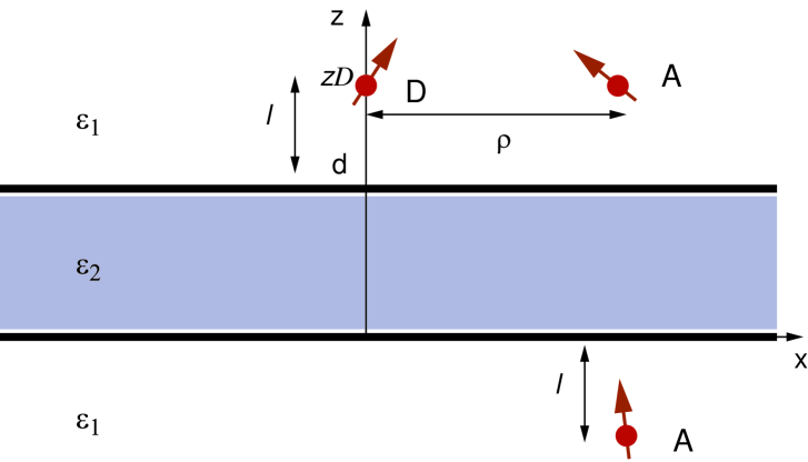
Figure 1: Schematic illustration of the system. Two graphene encapsulation layers of surface conductivity $\sigma$ are deposited on an embedded dielectric slab at $z=0$ and $z=d$. The donor D is located at $\textbf{x}=z_{D}\hat{z}$ ($z_{D}=d+l$) and acceptor A is located at $\textbf{x}=\rho\hat{\rho}+z_{D}\hat{z}$ (above the waveguide) or $\textbf{x}=\rho\hat{\rho}-l\hat{z}$ (below the waveguide).

In this approximation, the current density $\textbf{j}_{A}(\textbf{x})=-i\omega\textbf{p}_{A}\,\delta(\textbf{x}-\textbf{x}_{A})$ and, taking into account that the dipole moment $p_{A}$ is the induced dipole by the electric field $\textbf{E}_{D}$ generated by $p_{D}$, in the linear regime, Eq. (1) can be written as [31]

$$P_{ET}=\frac{\omega}{2}{\rm Im\mit}\left\{\alpha_{A}\right\}|\hat{n}_{A}\cdot\textbf{E}_{D}(\textbf{x}_{A})|^{2},$$ (2)

where $\alpha_{A}$ is the polarizability of the aceptor and $\hat{n}_{A}$ is a unit vector along the induced polarization of the acceptor (whose direction is supposedly to be fixed). The energy transfer rate normalized with respect to the power emitted in absence of the waveguide, $P_{0}=\frac{\omega p^{2}_{D}k_{1}^{3}}{3\varepsilon_{1}}$, is written as

$$\frac{P_{ET}}{P_{0}}={\rm Im\mit}\left\{\alpha_{A}\right\}T(\omega),$$ (3)

where

$$T(\omega)=\frac{3\varepsilon_{1}}{2k_{1}^{3}p_{D}^{2}}|\hat{n}_{A}\cdot\textbf{E}_{D}(\textbf{x}_{A})|^{2}$$ (4)

is the energy transfer function. The energy transfer in the presence of the graphene waveguide normalized to that in an unbounded medium 1 (without graphene waveguide), is given by

$$F_{ET}=\frac{T(\omega)}{T_{0}(\omega)},$$ (5)

with

$$T_{0}(\omega)=\frac{3\varepsilon_{1}}{2k_{1}^{3}p_{D}^{2}}|\hat{n}_{A}\cdot\textbf{E}_{0}(\textbf{x}_{A})|^{2},$$ (6)

where $\textbf{E}_{0}(\textbf{x}_{A})$ is the field generated by the donor at the acceptor position in the absence of the graphene waveguide.

The expression of the electric field $\textbf{E}_{0}(\textbf{x})$ due to an electric dipole in an unbounded medium is given in A, and a detailed sketch to obtain integral expressions for the electric field $\textbf{E}_{D}(\textbf{x})$ in the presence of a graphene waveguide is presented in B.

2.2 Case $\textbf{p}_{D}=p\hat{z}$

Firstly, we consider the case in which the donor dipole moment is oriented in the $\hat{z}$ direction. From Eq. (B18), it can be seen that $d_{p}=p$ and $d_{s}=0$ and, as a consequence, $A^{(1)}_{s}=B^{(3)}_{s}=0$. Even though Eqs. (B) and (B) give the electric field outside the waveguide straightforwardly, it is convenient to carry out their transformation to polar coordinates,

$$\alpha=k_{||}\cos\phi_{k},$$ (7)

$$\beta=k_{||}\sin\phi_{k}.$$ (8)

Taking into account the integral definition of the $0$th order of Bessel function

$$J_{0}(x)=\frac{1}{2\pi}\int_{0}^{2\pi}due^{ix\cos u},$$ (9)

and the recurrence relation

$$J^{\prime}_{m}(x)=\frac{1}{2}(J_{m-1}(x)-J_{m+1}(x)),$$ (10)

Eqs. (B) and (B) which give the scattered electric field expressions in medium 1 (above the waveguide) and in medium 2 (below the waveguide) can be rewritten as

$$\textbf{E}^{(1)}(\textbf{x})|_{scatt}=$$

$$\frac{ik_{0}^{2}}{k_{1}^{2}}\int_{0}^{+\infty}\left[\gamma^{(1)}\frac{J_{1}(k_{||}\rho)}{i}\hat{\rho}+k_{||}J_{0}(k_{||}\rho)\hat{z}\right]A^{(1)}_{p}e^{i\gamma^{(1)}z}k_{||}^{2}dk_{||},$$ (11)

and

$$\textbf{E}^{(3)}(\textbf{x})=$$

$$\frac{ik_{0}^{2}}{k_{1}^{2}}\int_{0}^{+\infty}\left[\gamma^{(1)}\frac{J_{1}(k_{||}\rho)}{i}\hat{\rho}+k_{||}J_{0}(k_{||}\rho)\hat{z}\right]B^{(3)}_{p}e^{-i\gamma^{(1)}z}k_{||}^{2}dk_{||}.$$ (12)

An integral of this kind represents a challenge due to the uncomfortable behavior of the integrand. To avoid this difficulty we have developed two methods to perform such integration. The first method requires the application of the residues theorem to extract each pole contribution of the integrals (2.2) and (2.2). The second method is carried out by using the Cauchy’s integral theorem in order to deform the path of integration into a suitable path in the complex $k_{||}$ plane. Then we use a Gauss–Legendre quadrature to evaluate the integrals along the deformed path.

2.2.1 Calculation of the graphene eigenmodes contribution

The integration path in Eqs. (2.2) and (2.2) is set along the real and positive $k_{||}$ axis, so that the integral will be strongly affected by singularities that are close to that axis. Pole singularities, i.e., zeroes of the denominator in $A_{p}^{(1)}$ and $B_{p}^{(3)}$ coefficients, occur at generally complex locations ($k_{||}$ is a complex magnitude) and they represent the propagation constant of the eigenmodes supported by the graphene waveguide, like waveguide (WG) or surface plasmon (SP) modes. The WG modes refer to modes which are evanescent waves in the two semi infinite regions (regions 1 and 3) and standing waves in the insulator spacer layer (region 2), and SPs refer to modes which propagate along the waveguide with their electric and magnetic fields decaying exponentially away from the graphene sheets in all three regions. These eigenmodes (especially SP modes) provide new decay channels for the electromagnetic energy transfer between single emitters placed close to the waveguide. For this reason, close attention must be paid to the calculation of their contribution to the field integrals (2.2) and (2.2) as well as to the resonance energy transfer (5). The integration method described in the present subsection makes use of the symmetry properties of the Bessel and Hankel functions [32] given by

$$J_{n}(x)=\frac{1}{2\pi}[H_{n}^{(1)}(x)+H_{n}^{(2)}(x)],$$

$$H_{n}^{(1)}(xe^{i\pi})=-e^{-in\pi}H_{n}^{(2)}(x).$$ (13)

Application of the symmetry properties (2.2.1) to the functions that form our integrands in (2.2) and (2.2), results in the following identities:

$$\int_{0}^{+\infty}f_{odd}(x)J_{0}(x)dx=\frac{1}{2}\int_{-\infty}^{+\infty}f_{odd}(x)H_{0}^{(1)}(x)dx,$$

$$\int_{0}^{+\infty}f_{even}(x)J_{1}(x)dx=\frac{1}{2}\int_{-\infty}^{+\infty}f_{even}(x)H_{1}^{(1)}(x)dx,$$ (14)

with

$$f_{odd}(x)=\frac{i}{\varepsilon_{1}}O\,k_{||}^{3},$$

$$f_{even}(x)=\frac{1}{\varepsilon_{1}}O\,\gamma^{(1)}k_{||}^{2}$$ (15)

where $O=A^{(1)}_{p}\,e^{i\gamma^{(1)}z}$ for the field components in Eq. (2.2) or $O=B^{(3)}_{p}\,e^{-i\gamma^{(1)}z}$ for the field components in Eq. (2.2). Therefore, Eqs. (2.2) and (2.2) can be rewritten as

$$\textbf{E}^{(1)}(\textbf{x})|_{scatt}=\frac{1}{2\varepsilon_{1}}\int_{-\infty}^{+\infty}\left[\gamma^{(1)}H_{1}^{(1)}(k_{||}\rho)\hat{\rho}+ik_{||}H_{0}^{(1)}(k_{||}\rho)\hat{z}\right]A^{(1)}_{p}$$

$$\times e^{i\gamma^{(1)}z}k_{||}^{2}dk_{||},$$ (16)

and

$$\textbf{E}^{(3)}(\textbf{x})=\frac{1}{2\varepsilon_{1}}\int_{-\infty}^{+\infty}\left[\gamma^{(1)}H_{1}^{(1)}(k_{||}\rho)\hat{\rho}+ik_{||}H_{0}^{(1)}(k_{||}\rho)\hat{z}\right]B^{(3)}_{p}$$

$$\times e^{-i\gamma^{(1)}z}k_{||}^{2}dk_{||}.$$ (17)

We now deform the integration path in (2.2.1) and (2.2.1) into a semicircle of large radius ($|k_{||}|\rightarrow\infty$) in the positive imaginary half–plane ${\rm Im\mit}k_{||}>0$, avoiding the branch point and pole singularities, as indicated in Figure 2a. The vertical lines drawn from the branch point $k_{1}=\sqrt{\varepsilon_{1}}$ to $+i\infty$ ($-k_{1}$ to $-i\infty$) are the branch cut lines. Since, $H_{n}(k_{||}\rho)\approx e^{ik_{||}\rho}/\sqrt{k_{||}\rho}$ for $k_{||}\rho$ large enough, the contribution along that semicircle vanishes. The integration along the branch cut $B_{1}$ results in a volume wave [33, 34], which consist of a continuous spectrum of radiation modes. On the contrary, the residue contributions correspond to eigenmodes propagating in the radial direction and with a discrete spectrum. In particular, we focus on distances between emitters smaller or of the same order than the propagation length of the waveguide eigenmodes. As a consequency, the intensity of the electric field reached by the excitation of these modes are orders of magnitude larger than that corresponding to the excitation of the volume wave modes. At these distances the energy transfer rate though eigenmodes is dominant and the volume wave mode contribution, which is in the order of the free space wave contribution, can be neglected. Then, the residues theorem gives

$$\textbf{E}^{(1)}(\textbf{x})|_{scatt}=\sum_{j}\textbf{E}^{(1)}_{j}(\textbf{x}),$$ (18)

where

$$\textbf{E}_{j}^{(1)}(\textbf{x})=\frac{1}{2\varepsilon_{1}}\left[\gamma_{j}^{(1)}H_{1}^{(1)}(k_{||,j}\rho)\hat{\rho}+ik_{||,j}H_{0}^{(1)}(k_{||,j}\rho)\hat{z}\right]e^{i\gamma_{j}^{(1)}z}k_{||,j}^{2}$$

$$\times 2\pi i\,\mbox{Res}A^{(1)}_{p}.$$ (19)

Similarly, the application of the residues theorem in Eq (2.2.1) gives

$$\textbf{E}^{(3)}(\textbf{x})=\sum_{j}\textbf{E}^{(3)}_{j},$$ (20)

$$\textbf{E}_{j}^{(3)}(\textbf{x})=\frac{1}{2\varepsilon_{1}}\left[\gamma_{j}^{(1)}H_{1}^{(1)}(k_{||,j}\rho)\hat{\rho}+ik_{||,j}H_{0}^{(1)}(k_{||,j}\rho)\hat{z}\right]e^{-i\gamma_{j}^{(1)}z}k_{||,j}^{2}$$

$$\times 2\pi i\,\mbox{Res}B^{(3)}_{p},$$ (21)

where $k_{||,j}$ is the propagation constant of a particular eigenmode, $j=$sp for SPs (ASPs or SSPs) or $j=$wg for WG modes (both quantities higher than the modulus of the photon wave vector in media 1 and 3), and Res is the residue of the integrand in (2.2.1) and (2.2.1) at the pole $k_{||,j}$.

$$\mbox{Res}A_{p}^{(1)}=\lim_{k_{||}\to k_{||,j}}(k_{||}-k_{||,j})A_{p}^{(1)},$$

$$\mbox{Res}B_{p}^{(3)}=\lim_{k_{||}\to k_{||,j}}(k_{||}-k_{||,j})B_{p}^{(3)}.$$

Inserting the expressions for $\textbf{E}^{(1)}(\textbf{x})|_{scatt}$ and $\textbf{E}^{(3)}(\textbf{x})$ given by Eqs. (18) and (20) into Eq. (5) we obtain the following expression for the normalized energy transfer rate,

$$F_{ET}=\sum_{lj}F_{lj}=\sum_{lj}\frac{T_{lj}(\omega)}{T_{0}(\omega)},$$ (23)

where

$$F_{lj}=\frac{T_{lj}(\omega)}{T_{0}(\omega)}=\frac{\hat{n}_{A}\cdot\textbf{E}_{l}(\textbf{x}_{A})\,\hat{n}_{A}\cdot\textbf{E}_{j}^{*}(\textbf{x}_{A})}{|\hat{n}_{A}\cdot\textbf{E}_{0}(\textbf{x}_{A})|^{2}}.$$ (24)

Note that $F_{jj}$ is the contribution of the $j$ eigenmode channel to the normalized energy transfer rate whereas $F_{l\not=j}$ corresponds to interference terms between $l$ and $j$ channels.

2.2.2 Direct integration. Numerical quadrature

In this subsection we transform the original oscillatory integrand function into one to avoid the complex singularities which lie near the real $k_{||}$ axis and then we apply a numerical quadrature to calculate the field integrals. This procedure does not require to determine the location of each pole, i.e., the determination of the complex propagation constant of the graphene waveguide. Unlike the method described in section 2.2.1 which allows to calculate separately the contribution of each one of the eigenmodes to the electric field, the present method only allows to calculate the total electric field scattered by the graphene waveguide. To do this, we follow a procedure similar to one developed in [35]. We surround the pole singularities by deforming the integration path into the complex plane as shown in Figure 2. The path I is an elliptical path starting at $k_{||}=0$ with the major semi–axis $k_{||}=a$ and the minor semi–axis $k_{||}=b$. In the region between path I and the real axis the integrand function is analytical, thus the Cauchy’s integral theorem implies that an integration on path I will be equal to the integral on the real axis from 0 to $2a$. The $a$ value should be chosen large enough to surround all pole singularities, thus $2a>\alpha_{\mbox{\tiny{ssp}}}$ must be fulfilled. Unlike the dielectric or metallic waveguides, the propagation constant of the symmetric surface plasmon $\alpha_{\mbox{\tiny{ssp}}}$ on a graphene waveguide can reach values up to two orders of magnitude greater than that corresponding to a photon of the same frequency. Therefore, in a first step it is necessary to divide the integration interval into several subintervals and then to apply the numerical quadrature in each subinterval.

Taking into account the symmetry properties (2.2.1) and the fact that the Hankel funtions of the first kind $H_{n}^{(1)}(z)$ and the second kind $H_{n}^{(2)}(z)$ decrease faster as long as $|{\rm Im\mit}z|$ increases in the sector ${\rm Im\mit}z>0$ and ${\rm Im\mit}z<0$, respectively, the remaining integration is carried out by deflecting the integration path from the real axis to a path parallel to the imaginary $k_{||}$ axis as shown in Figure 1, with ${\rm Im\mit}k_{||}>0$ for $H_{n}^{(1)}(k_{||}\rho)$ (path II) and with ${\rm Im\mit}k_{||}<0$ for $H_{n}^{(2)}(k_{||}\rho)$ (path III). In the region between path II and the real axis the integrand has no pole singularities, thus Cauchy’s integral theorem implies that the integral on a closed path in this region will be zero.Therefore, the integral over path II in the direction shown in Figure 1 is equal to that from $2a$ to$+\infty$ over the real axis. In a similar way, one can demonstrate that the integral over path III in the direction shown in Figure 1 is equal to that from $2a$ to$+\infty$ over the real axis. In our implementation, we have used a 32 point Gauss Legendre quadrature to calculate the field integrals on paths I, II and III.

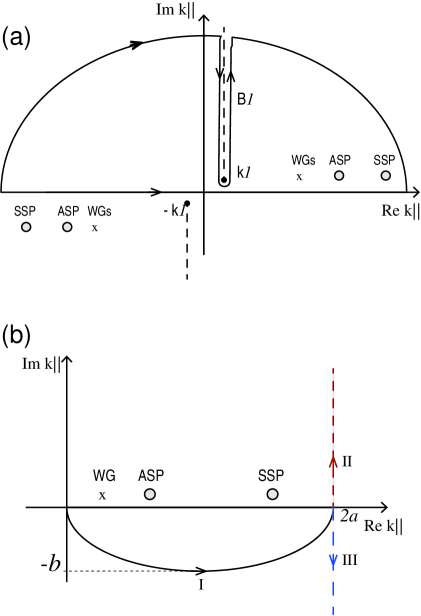
Figure 2: Singularities and path of integration in the complex plane $k_{||}={\rm Re\mit}k_{||}+i{\rm Im\mit}{k_{||}}$ for the electromagnetic fields. (a) Integration path, vertical branch cuts and poles captured. (b) The original path, along the positive semi–axis, is deformed along an elliptical path (I) surrounding the singularities, together with the paths (II) and (III) parallel to the imaginary $k_{||}$ axis using Hankel functions.

2.3 Case $\textbf{p}_{D}=p\hat{\rho}$

We next consider the case in which the donor dipole moment is oriented parallely to the graphene waveguide. Without loss of generality, we suppose this orientation in the $x$ axis. From Eq. (B18), results,

$$d_{p}^{-}=\frac{\alpha\gamma^{(1)}}{\alpha^{2}+\beta^{2}}p$$

$$d_{s}^{-}=-\frac{k_{0}\gamma^{(1)}}{\alpha^{2}+\beta^{2}}p.$$ (25)

Following a similar way to that used to obtain Eqs. (B) and (B), we obtain the follow expressions for the electric field components below to the waveguide

$$E^{(3)}(\textbf{x})|_{\rho}=\frac{i}{2\varepsilon_{1}}\int_{-\infty}^{+\infty}\left[-H_{0}^{(1)}(k_{||}\rho)+\frac{H_{1}^{(1)}(k_{||}\rho)}{\rho}\right]\cos\phi\,B^{(3)}_{p}$$

$$\times e^{-i\gamma^{(1)}z}(\gamma^{(1)})^{2}\,k_{||}dk_{||},$$ (26)

$$E^{(3)}(\textbf{x})|_{\phi}=\frac{i}{2\varepsilon_{1}}\int_{-\infty}^{+\infty}[(\gamma^{(1)})^{2}\frac{H_{1}^{(1)}(k_{||}\rho)}{\rho}\,\sin\phi\,B^{(3)}_{p}$$

$$+\frac{k_{1}^{2}}{i}H_{1}^{(1)}(k_{||}\rho)\,B^{(3)}_{s}]\,e^{-i\gamma^{(1)}z}\,k_{||}dk_{||},$$ (27)

$$E^{(3)}(\textbf{x})|_{z}=-\frac{1}{2\varepsilon_{1}}\int_{-\infty}^{+\infty}H_{1}^{(1)}(k_{||}\rho)\,B^{(3)}_{p}\cos\phi e^{-i\gamma^{(1)}z}\gamma^{(1)}k_{||}^{2}dk_{||},$$ (28)

with similar expressions for the scattered electric field on the region located above the waveguide (medium 1). The residues theorem applied to these field components gives

$$\textbf{E}^{(3)}(\textbf{x})=\sum_{j}\textbf{E}^{(3)}_{j},$$ (29)

$$\begin{array}[]{ll}\textbf{E}_{j}^{(3)}(\textbf{x})=\frac{i}{2\varepsilon_{1}}[\gamma_{j}^{(1)}\left(-H_{0}^{(1)}(k_{||,j}\rho)+\frac{H_{1}^{(1)}(k_{||,j}\rho)}{\rho}\right)\cos\phi\,\hat{\rho}\\ +\gamma_{j}^{(1)}\frac{H_{1}^{(1)}(k_{||,j}\rho)}{\rho}\,\sin\phi\,\hat{\phi}+i\,k_{||,j}H_{1}^{(1)}(k_{||,j}\rho)\cos\phi\,\hat{z}]\\ \times e^{-i\gamma_{j}^{(1)}z}k_{||,j}\gamma_{j}^{(1)}\,2\pi i\,\mbox{Res}B^{(3)}_{p},\end{array}$$

where $k_{||,j}$ is the propagation constant of SPs, $j=$ASP, SSP. Note that, for this dipole orientation, there are $s$ and $p$ polarized decay channels involved in the first and in the second term in Eq. (2.3), respectively. However, only $p$ polarized SPs exist in the graphene waveguide at the considered frequency range, and as a consequence only the first term contribute to the SP field. On the other hand, as in the vertical dipole orientation, we have neglected the contribution of the volume wave electric field in Eq. (29) to the energy transfer rate.

3 Results

In this section we apply the formalism developed in previous sections to calculate the energy transfer rate between two emitters localized close to a graphene waveguide. In order to obtain separate contributions of different eigenmodes, firstly we obtain the propagation constant of these modes by requiring the denominator in the amplitudes $A_{p}^{(1)}$ and $B_{p}^{(3)}$ to be zero [30]. Due to the high spatial confinement of SPs in comparison with that of the WG modes, the energy transfer through the graphene waveguide due to excitation of SPs is much greater than the corresponding energy transfer through the excitation of WG modes [20, 30]. Thus, as we have verified, the ASP and SSP contributions dominate the energy transfer process on the frequency region presented in Figure 3 (where the SPs are well defined) and consequently the WG contributions can be neglected in Eq. (23). Since the imaginary part of the graphene conductivity (see C) ${\rm Im\mit}\sigma$ changes sign from positive to negative at $\omega/\mu_{c}\approx 1.667$, due to the presence of the interband term in the conductivity, $p$–polarized SPs are well defined on the frequency range below such frequency.

Figure 3 shows the propagation constant $k_{||}$ of the antisymmetric surface plasmon (ASPs) and symmetric surface plasmon (SSPs) as a function of the frequency $\omega/c$ for $\mu_{c}=0.4$eV and $d=0.02\mu$m. With this value of $\mu_{c}$, $p$–polarized SPs are supported by the structure for frequency values less than $\approx 3\mu$m^-1. To appreciate the details of the dispersion SP curves, they are plotted in the range $\omega/c<2\mu$m^-1. Since the fields of these modes strongly overlap inside the thin layer (medium 2), the dispersion curves result in two well separated branches. The upper branch corresponds to the ASP mode and the lower branch corresponds to the SSP mode. At high frequencies, $\omega/c>2\mu$m^-1, SPs of the two graphene sheets are essentially uncoupled from each other and both the symmetric and the antisymmetric branches merge into the dispersion curve of the single SP mode supported by a graphene sheet.

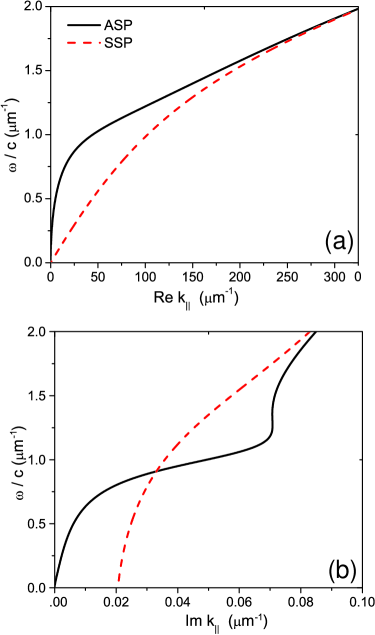
Figure 3: Dispersion curves for SSP and ASP modes, calculated for $\mu_{c}=0.4$eV, $T=300$ K, $\gamma_{c}=0.1$meV, $\varepsilon_{1}=1$ and $\varepsilon_{2}=3.9$. (a) ${\rm Re\mit}k_{||}$ and (b) ${\rm Im\mit}k_{||}$ as a function of $\omega/c$.

Once the propagation constants are determined, the contribution of each SP modes to the total energy transfer rate has been calculated by the residues method (18). Firstly, we briefly consider the case when the pair of donor and acceptor dipoles are on the same side of the graphene waveguide, and located at a distance $l$ from this one. Then, we consider the more realistic case when the donor and acceptor are placed on opposite sides on the waveguide. We focus on three configurations: the dipole moments are oriented perpendicular to the waveguide, the dipole moment of the donor is perpendicular to the waveguide and that of the acceptor is parallel to the waveguide, both dipole moments of donor and acceptor are parallel to the waveguide and parallel to each other, and both dipole moments of donor and acceptor are parallel to the waveguide and perpendicular to each other.

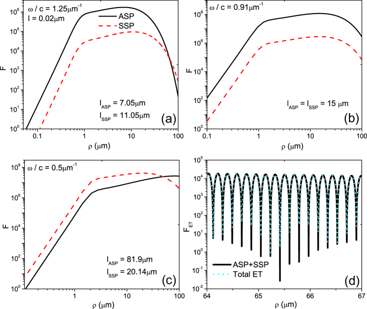
Figure 4: Contribution of the ASP and the SSP, $F_{\mbox{\tiny{ASP,ASP}}}$ and $F_{\mbox{\tiny{SSP,SSP}}}$, to the normalized energy transfer rate between two dipoles, both placed at the same $z=0.04\mu$m axis (at a distance $l=z_{D}-d=0.02\mu$m from the surface of the graphene waveguide), as a function of the in–plane separation $\rho$. The frequency $\omega/c=1.25\mu$m^-1 (a), $\omega/c=0.91\mu$m^-1 (b) and $\omega/c=0.5\mu$m^-1 (c), and the dipole moments are oriented along the $z$ axis. (d) Normalized total energy transfer rate and the superposition of the ASP and SSP as a function of the in–plane distance between the donor and acceptor. The waveguide parameters are the same as in Figure 3.

In Figure 4 we have plotted the contribution of the SP modes to the normalized energy transfer rate, i.e., the energy transfer terms in (24) with $l=j=$ASP and $l=j=$SSP ($F_{\mbox{\tiny{ASP,ASP}}}$ and $F_{\mbox{\tiny{SSP,SSP}}}$), as a function of the in–plane separation between the donor and acceptor and for several $\omega/c=1.25,\,0.91,\,\mbox{and}\,0.5\mu$m^-1 frequency transition values. The donor and acceptor are localized on the same side of the waveguide (medium 1), at $\textbf{x}_{D}=0.04\mu$m$\hat{z}$ and $\textbf{x}_{A}=\rho\hat{\rho}+0.04\mu$m$\hat{z}$, respectively, and with their dipole moments aligned along the $z$ axis. In all the cases, the normalized energy transfer contributions is larger than 10, pointing out that SP excitations dominate the energy transfer process in the distance range considered in Figure 4. At larger distances the imaginary part of the SPs propagation constant turns out an exponentially decaying field and, as a consequence the energy transfer begins to be dominated by the free–space radiation [not shown in Figure 4]. As in the single graphene sheet case, we have verified that the crossover distance occurs at $\approx 10L-20L$ [29] where $L=\frac{1}{2{\rm Im\mit}\,\alpha_{\mbox{\tiny{SP}}}}$ is the propagation length of SPs.

In Figure 4a, we observe that the maximum value of the normalized energy transfer rate for the SSP falls at $\rho_{max}\approx 11\mu$m, a value that is larger than that corresponding to the ASP, $\rho_{max}\approx 7\mu$m. On the other hand, by using the calculated ${\rm Im\mit}\,\alpha_{\mbox{\tiny{SP}}}$ values plotted in Figure 3b for $\omega/c=1.25\mu$m^-1, we have obtained $L_{\mbox{\tiny{SSP}}}=11.05\mu$m and $L_{\mbox{\tiny{ASP}}}=7.05\mu$m for the SSP and the ASP, respectively, which agree well with $\rho$ values where the energy transfer reaches its maximum value. The correspondence between the position of these maxima and the propagation length of SPs, which has been reported in [26] for the case of single graphene sheet, can be understood as follows: since the $\hat{z}$–component of the SP electric field (2.2.1) depends on the $\rho$ distance as $E_{\mbox{\tiny{sp}},z}(\rho)\approx H_{0}^{(1)}(\alpha_{\mbox{\tiny{SP}}}\rho)$, for argument values large enough, $\alpha_{\mbox{\tiny{SP}}}\rho>>1$, it follows that

$$E_{\mbox{\tiny{SP}},z}(\rho)\approx\frac{e^{i\alpha_{\mbox{\tiny{SP}}}\,\rho}}{\sqrt{\rho}}=\frac{e^{i{\rm Re\mit}\alpha_{\mbox{\tiny{SP}}}\,\rho-{\rm Im\mit}\alpha_{\mbox{\tiny{SP}}}\,\rho}}{\sqrt{\rho}}.$$ (30)

Taking into account that, in the absence the graphene waveguide, the field of the donor is written as (refer to A for its derivation)

$$E_{0,z}(\rho)=\frac{e^{ik_{1}\rho}}{\rho},$$ (31)

it follows that the energy transfer contribution of either of the two SP channels (2.2.1) can be written as

$$F_{\mbox{\tiny{SP}}}=|\frac{E_{\mbox{\tiny{SP}},z}(\rho)}{E_{0,z}(\rho)}|^{2}=\rho e^{-2{\rm Im\mit}\alpha_{\mbox{\tiny{SP}}}\,\rho},$$ (32)

which reaches its maximum value at $\rho=\frac{1}{2{\rm Im\mit}\alpha_{\mbox{\tiny{SP}}}}$. From this fact and taking into account the values of ${\rm Im\mit}\alpha_{\mbox{\tiny{SP}}}$ calculated in Figure 3b, we conclude that for frequency values less (greater) than $0.91\mu$m^-1, the curve of $F_{\mbox{\tiny{ASP,ASP}}}$ reaches its maximum value at a distance greater (less) than that corresponding to the curve of $F_{\mbox{\tiny{SSP,SSP}}}$. Figures 4a–c confirm such behavior.

It is worth noting that the energy transfer rate between the donor and acceptor arises from a coherent superposition of the ASP and the SSP contributions (both calculated in Figures 4a–c) into Eq. (23), leading to a spatial modulation due to interference terms $F_{lj}$ with $l=\mbox{ASP},\,j=\mbox{SSP}$ and $l=\mbox{SSP},\,j=\mbox{ASP}$. This fact is illustrated in Figure 4d where we have plotted the normalized energy transfer rate for $\omega/c=1.25\mu$m^-1 by considering only the SP terms in Eq. (23), on the one hand, and by direct integration, i.e., by using Eq. (2.2.1) as explained in subsection 2.2.2, on the other hand. We see that both curves match, confirming that the energy transfer rate is well approximated by the coherent superposition of both ASP and SSP mode channels provided that the in–plane separation between the donor and acceptor is comparable or even lower than the SP propagation length. In order to visualize a strong interference effect, in Figure 4c we have plotted the energy transfer curve for a distance range close to $65\mu$m in which the ASP and the SPP energy transfer contributions are approximately equals to each other, as can be seen in Figure 4a. We observe a pronounced spatial oscillation whose period $\Lambda\approx 0.185\mu$m, a value that can be calculated within the framework of the model in Eq. (23), where the interference term between the SSP and ASP is written as

$$I=F_{\mbox{\tiny{SSP}},\mbox{\tiny{ASP}}}+F_{\mbox{\tiny{ASP}},\mbox{\tiny{SSP}}}\approx\cos[({\rm Re\mit}\alpha_{\mbox{\tiny{SSP}}}-{\rm Re\mit}\alpha_{\mbox{\tiny{ASP}}})\rho].$$ (33)

Equation (33) shows a periodic spatial dependence along $\rho$ direction with a period $\Lambda=2\pi/({\rm Re\mit}\alpha_{\mbox{\tiny{SSP}}}-{\rm Re\mit}\alpha_{\mbox{\tiny{ASP}}})=2\pi/(142.2\mu\mbox{m}^{-1}-108.2\mu\mbox{m}^{-1})\approx 0.1847\mu$m, where we have used the values of the SP propagation constants calculated in Figure 3a for $\omega/c=1.25\mu$m^-1.

We now consider the SP coupling efficiency supporting the energy transfer between donor and acceptor on opposite sides of the graphene waveguide. As in the metallic slab case [1, 3], we expect that the electromagnetic field extending between the two graphene layers of the waveguide being able to facilitate the energy transfer between dipoles placed on opposite sides of the waveguide.

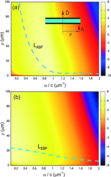
Figure 5: Map of the SP contributions $F_{\mbox{\tiny{ASP,ASP}}}$ (a) and $F_{\mbox{\tiny{SSP,SSP}}}$ (b) as a function of frequency and the in–plane distance between the donor and acceptor. The dashed line curves correspond to the propagation lengths of SPs. The donor and acceptor are localized on opposite sides of the waveguide, $z_{D}=0.04\mu$m (at a distance $l=0.02\mu$m from the top of the waveguide) and $z_{A}=-0.02\mu$m (at a distance $l=0.02\mu$m from the bottom of the waveguide), with their dipole moments along the $z$ axis. The waveguide parameters are the same as in Figure 3.

Our calculations confirm this expectation, as can be seen in Figure 5 where we show plots of the SP contributions to the normalized energy transfer rate, $F_{\mbox{\tiny{ASP,ASP}}}$ and $F_{\mbox{\tiny{SSP,SSP}}}$, as a function of the in–plane distance $\rho$ and $\omega/c$ frequency for the case where the donor is placed at $\textbf{x}_{D}=0.04\mu$m $\hat{z}$ (above the waveguide) and the acceptor is placed at $\textbf{x}_{A}=\rho\hat{\rho}-0.02\mu$m$\hat{z}$ (below the waveguide). The electric dipole of the donor and acceptor are oriented along the $z$ axis. As in the previously presented case where the donor and acceptor were localized on the same side of the waveguide, we also observe that the maximum normalized energy transfer rate is obtained for a value of the in–plane separation close to the propagation length of the SP.

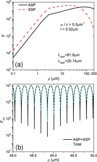
Figure 6: Contribution of the ASP and the SSP, $F_{\mbox{\tiny{ASP,ASP}}}$ and $F_{\mbox{\tiny{SSP,SSP}}}$ (a), to the normalized energy transfer rate between D and A placed on opposite sides of the waveguide as a function of the $\rho$ distance between them. (b) Normalized total energy transfer rate and the superposition of the ASP and SSP as a function of the distance between D and A dipoles. The transition frequency $\omega/c=0.5\mu$m^-1 and the dipole moments are oriented along the $z$ axis. The waveguide parameters and the location of D and A are the same as in Figure 5.

To appreciate the spatial details of the SP energy transfer from donor to acceptor, in Figure 6a we have plotted the ASP and SSP contributions as a function of the in–plane $\rho$ separation for $\omega/c=0.5\mu$m^-1. Since the frequency value $\omega/c<1\mu$m^-1, the ASP contribution curve exhibits its maximum value at an in–plane separation greater than that corresponding to the SSP contribution curve ($\rho_{max,\mbox{\tiny{ASP}}}=81.9\mu$m and $\rho_{max,\mbox{\tiny{SSP}}}=20.14\mu$m). Figure 6b shows the normalized total energy transfer rate $F_{ET}$ calculated by direct integration as it has been described in section 2.2.2, and by the coherent superposition of the ASP and SSP channels to the normalized energy transfer (23), for distance values close to $49\mu$m (where the ASP and SSP energy transfer contributions are approximately the same). We observe a great spatial modulation due to the interference effect between the ASP and SSP whose period $\Lambda\approx 0.16\mu$m, a value that can be obtained by using the propagation constant values shown in Figure 3a for $\omega/c=0.5\mu$m^-1, $\Lambda=2\pi/({\rm Re\mit}\alpha_{\mbox{\tiny{SSP}}}-{\rm Re\mit}\alpha_{\mbox{\tiny{ASP}}})=2\pi/(44.055\mu$m${}^{-1}-5.085\mu$m${}^{-1})\approx 0.1612\mu$m^-1.

To further investigate the effect that the variation of the chemical potential has on the energy transfer rate, we specify the in–plane separation between the donor and acceptor and vary the chemical potential $\mu_{c}$. Even though $\mu_{c}$ variations are manifested as a significant energy transfer modification in the whole range of the donor–acceptor separation considered in Figure 6, for the sake of clarity we have chosen $\rho=48.85\mu$m, a value for which the total energy transfer rate exhibits an absolute minimum value (Figure 6b). Figure 7 shows a plot of the normalized total energy transfer $F_{ET}$ as a function of the chemical potential $\mu_{c}$ for the same configuration as in Figure 6.

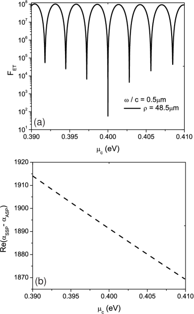
Figure 7: (a) Total energy transfer rate $F_{ET}$ between donor and acceptor placed on opposite sides of the waveguide as a function of the chemical potential $\mu_{c}$. (b) $\Delta\alpha_{\mbox{\tiny{SP}}}(\mu_{c})$ for $\mu_{c}$ values near to $\mu_{c}=0.4$eV. The frequency $\omega/c=0.5\mu$m^-1, the dipole moments are oriented along the $z$ axis and the in–plane separation is set at $\rho=48.5\mu$m. The waveguide parameters are the same as in Figure 6.

We observe that, by varying the chemical potential from $0.4$eV, the normalized energy transfer rate notably increases, near six orders of magnitude, towards values close to $10^{8}$. Then, $F_{ET}$ decreases towards another minimum and follows the same behavior, almost periodically, as the chemical potential modulus is increased. The period of the oscillations, determined by the distance between two consecutive minima in Figure 7a, is $\Lambda_{\mu}\approx 0.0028$eV. The origin of this periodic behavior is explained by Eq. (33) where the argument of the interference term $\varphi(\mu_{c})=\Delta\alpha_{\mbox{\tiny{SP}}}(\mu_{c})\,\rho$ ($\Delta\alpha_{\mbox{\tiny{SP}}}={\rm Re\mit}\alpha_{\mbox{\tiny{SSP}}}(\mu_{c})-{\rm Re\mit}\alpha_{\mbox{\tiny{ASP}}}(\mu_{c})$) is a function of $\mu_{c}$. In Figure 7b we have plotted $\Delta\alpha_{\mbox{\tiny{SP}}}$ as a function of $\mu_{c}$ in the range $0.39$eV$<\mu_{c}<0.41$eV. In this range, $\Delta\alpha_{\mbox{\tiny{SP}}}$ is a linear function of $\mu_{c}$ and as a consequence the argument can be approximated by $\varphi(\mu_{c})=\varphi(\mu^{(0)}_{c})+\Delta\alpha_{\mbox{\tiny{SP}}}^{\prime}(\mu^{(0)}_{c})\,(\mu_{c}-\mu^{(0)}_{c})\,\rho$, where $\mu^{(0)}_{c}=0.4$eV, $\Delta\alpha_{\mbox{\tiny{SP}}}^{\prime}(\mu^{(0)}_{c})=\Delta\alpha_{\mbox{\tiny{SP}}}^{\prime}(0.4$eV$)$ is the derivative with respect to $\mu_{c}$ and $\varphi(\mu^{(0)}_{c})=\Delta\alpha_{\mbox{\tiny{SP}}}(0.4$eV$)\,\rho$. Therefore, the period of the interference function (33) is $\Lambda_{\mu}=2\pi/[\Delta\alpha_{\mbox{\tiny{SP}}}^{\prime}(0.4$eV$)\,\rho]$. From Figure 7b we determine $\Delta\alpha_{\mbox{\tiny{SP}}}^{\prime}(0.4$eV$)=-46.125\mu$m^-1eV^-1, thus for $\rho=48.853\mu$m it follows that $\Lambda_{\mu}=2\pi/2253.23\,$eV$\approx 0.002788$eV, a value that agrees well with that previously determined value.

We next consider the configuration in which the orientation of the acceptor dipole is along the $\rho$ axis as it is shown in the inset of Figure 8a. We observe that both $F_{\mbox{\tiny{ASP,ASP}}}$ and $F_{\mbox{\tiny{SSP,SSP}}}$ curves exhibit a maximum value at approximately the same in–plane separation $\rho$ when frequency is $\omega/c=1\mu$m^-1.

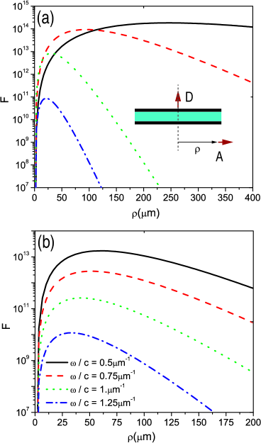
Figure 8: ASP and SSP contributions, $F_{\mbox{\tiny{ASP,ASP}}}$ (a) and $F_{\mbox{\tiny{SSP,SSP}}}$ (b), to the normalized energy transfer rate between D and A placed on opposite sides of the waveguide as a function of the $\rho$ distance between them. The dipole moments are oriented along the $z$ axis (donor) and along the $x$ axis (acceptor). The waveguide parameters and the location of D and A are the same as in Figure 5.

However, unlike the previous configuration (both donor and acceptor dipole moments aligned along the $z$ axis), the distance $\rho_{max}(1\mu$m${}^{-1})\approx 35\mu$m, a value representing threefold the SP propagation length ($L(1\mu$m${}^{-1})\approx 12\mu$m). In addition, we have verified the same behavior for all frequencies. This fact can be understood by taking into account that, in the absence of the graphene waveguide, the $\hat{x}$–component of the donor electric field is written as (see A)

$$E_{0,x}(\rho)=\frac{e^{ik_{1}\rho}}{\rho^{2}},$$ (34)

while the $\hat{x}$–component of the SP electric field is as in Eq. (30), $E_{\mbox{\tiny{SP}},x}(\rho)\approx E_{\mbox{\tiny{SP}},z}$. Thus, the energy transfer contribution of the SP channel (2.2.1) can be written as

$$F_{\mbox{\tiny{SP}}}=|\frac{E_{\mbox{\tiny{SP}},x}(\rho)}{E_{0,x}(\rho)}|^{2}=\rho^{3}e^{-2{\rm Im\mit}\alpha_{\mbox{\tiny{SP}}}\,\rho},$$ (35)

which reaches its maximum value at $\rho=\frac{3}{2{\rm Im\mit}\alpha_{\mbox{\tiny{SP}}}}=3L_{\mbox{\tiny{SP}}}$.

In addition to considering the energy transfer rate for the donor dipole moment aligned along the $z$ axis, another useful configuration is that in which the donor electric dipole lies parallel to the graphene waveguide. The acceptor is placed at the $z=-0.02\mu$m^-1 plane (below the waveguide). The position of the donor is fixed at $\textbf{x}_{D}=0.04\mu$m$\hat{z}$ (above the waveguide) and its projection on the acceptor plane is indicated with an arrow in Figure 9. Without loss of generality we have chosen the donor orientation along the $x$ axis ($\textbf{p}_{D}=p\hat{x}$). Figure 9 shows the spatial distribution of the ASP contribution to the energy transfer function $T$ as a function of the acceptor position $(x,\,y)$ on $z=-0.02\mu$m^-1 plane. The frequency transition of the donor is chosen to be $\omega/c=1\mu$m^-1. The color map is calculated for the acceptor placed in each point of the plot. Unlike the case that we previously studied (when the donor orientation is parallel to the $z$ axis) for which both the transfer function $T$ and the unbounded transfer function $T_{0}$ are invariant under rotation around the $z$ axis, in the present case neither $T$ nor $T_{0}$ are invariant under rotation around the $z$ axis, although the $T/T_{0}$ rate (and as a consequence also $F$) is itself invariant. For this reason, and to highlight the symmetry of the energy transfer in the acceptor plane, we believe that the calculation of $T$ is particularly appropriate.

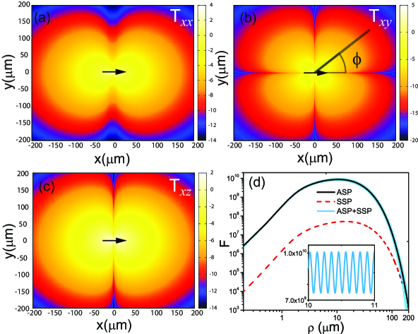
Figure 9: ASP contribution, $F_{\mbox{\tiny{ASP,ASP}}}$, to the energy transfer function $T$ (in logarithmic scale) between D and A placed on opposite sides of the waveguide ($\textbf{x}_{D}=0.04\mu$m$\hat{z}$ and $\textbf{x}_{A}=x\hat{x}+y\hat{y}-0.02\mu$m$\hat{z}$) as a function of the $x$ and $y$ axis on the $z=-0.02\mu$m plane (where A is placed). The dipole moment of D is along the $x$ axis and the dipole moment of A is along the $x$ axis (a), the $y$ axis (b) and the $z$ axis (c). (d) ASP and SSP contributions to the normalized energy transfer rate as a function of the distance $\rho$ along the line at $\phi=45^{\circ}$ in Figure 9b. The waveguide parameters and the location of D and A are the same as in Figure 5.

From Figure 9 we can see that the energy transfer rate presents a strongly angular dependence. For instance, Figure 9b shows four zones on the $z=-0.02\mu$m plane in which the energy transfer rate is enhanced. These zones appear limited by two lines $x=0$ and $y=0$ where the component of the donor electric field that lies parallel to the acceptor plane is in the $\hat{x}$ direction. As a consequence the energy transfer to the acceptor positioned at these lines with its dipole moment along the $\hat{y}$ direction is zero as can be seen in Figure 9b. On the other hand, the energy transfer to the acceptor oriented in the $z$ axis presents two enhanced zones limited by the $x=0$ line (Figure 9c), where the $\hat{z}$ component of the donor electric field is zero.

Since the imaginary part of the propagation constant value of the SSP at $\omega/c=1\mu$m^-1 is approximately the same as the ASP, the map corresponding to the SSP [not shown in Figure 9] is similar to that in Figure 9 for the ASP.

In order to highlight the role of SPs in the energy transfer rate, we calculate the ASP and the SSP contributions to the normalized energy transfer $F_{ET}$ along the line in Figure 9b with $\phi=45^{\circ}$. The acceptor dipole moment lies parallel to the $y$ axis. Figure 9d shows that the maximum value of the ASP contribution curve is near three orders of magnitude larger than the value obtained for the SSP contribution, a fact occurring in the whole acceptor plane regardless the $\phi$ angle. Both ASP and SSP curves exhibit their maximum values almost at the same $\rho_{max}$ distance, a fact that follows from the similarity between the imaginary parts of the ASP and SSP propagation constant at $\omega/c=1\mu$m^-1. Furthermore, this value is $\rho_{max}\approx 12\mu$m, which agrees well with that of the SP propagation length at this frequency. This is true because the $\hat{y}$ component of the SP electric field (ASP or SSP) given by Eq. (2.3) for $\phi=45^{\circ}$ and for long argument is $E_{\mbox{\tiny{SP}},y}(\rho)\approx\frac{e^{i\alpha_{\mbox{\tiny{SP}}}\,\rho}}{\sqrt{\rho}}$, whereas the $\hat{y}$ component of the electric field for the same dipole in an unbounded medium is $E_{0,y}(\rho)\approx\frac{e^{ik_{1}\rho}}{\rho}$. Therefore, $F=\frac{|E_{\mbox{\tiny{SP}},y}|^{2}}{|E_{0,y}(\rho)|^{2}}\approx\rho e^{-2{\rm Im\mit}\alpha_{\mbox{\tiny{SP}}}\,\rho}$ which reaches its maximum value at $\rho=\frac{1}{2{\rm Im\mit}\alpha_{\mbox{\tiny{SP}}}}=L_{\mbox{\tiny{SP}}}$. We have verified [not shown in Figure 9] that in the case that the electric dipole of the acceptor is set along the $z$ axis both ASP and SSP contribution curves exhibit their maximun values at $\rho_{max}\approx 35\mu$m, a value threefold larger than the SP propagation length $L(1\mu$m$)=12\mu$m. This fact can be explained by taking into account that the $\hat{z}$ component of the SP electric field (ASP or SSP) given by Eq. (2.3) for $\phi=45^{\circ}$ and for long argument is $E_{\mbox{\tiny{SP}},z}(\rho)\approx\frac{e^{i\alpha_{\mbox{\tiny{SP}}}\,\rho}}{\sqrt{\rho}}$, whereas the $\hat{z}$ component of the electric field for the same dipole in an unbounded medium is $E_{0,z}(\rho)\approx\frac{e^{ik_{1}\rho}}{\rho^{2}}$. Thus, $F=\frac{|E_{\mbox{\tiny{SP}},z}|^{2}}{|E_{0,z}(\rho)|^{2}}\approx\rho^{3}e^{-2{\rm Im\mit}\alpha_{\mbox{\tiny{SP}}}\,\rho}$ which reaches its maximum value at $\rho=\frac{3}{2{\rm Im\mit}\alpha_{\mbox{\tiny{SP}}}}=3L_{\mbox{\tiny{SP}}}$. We also observe interference oscillations in the total energy transfer curve, which agree well with the curve obtained by the coherent superposition between ASP and SSP modes. At low distances, where the main contribution to the energy transfer rate comes from the ASP, the interference effects are less pronounced than the corresponding effects at large distances, where the ASP and SSP contributions are similar. To appreciate the details of the interference between SP channels, in the inset of Figure 9d we have enlarged the horizontal scale of such figure. In the inset it is clearly shown that the oscillations present a spatial period $\Lambda\approx 0.11\mu$m, a value that agrees well with that calculated by using the real parts of SPs obtained in Figure 3a for $\omega/c=1\mu$m^-1, $\Lambda=2\pi/({\rm Re\mit}\alpha_{\mbox{\tiny{SSP}}}-{\rm Re\mit}\alpha_{\mbox{\tiny{SSP}}})\approx 2\pi/(102.4\mu\mbox{m}^{-1}-44.4\mu\mbox{m}^{-1})=0.108\mu$m.

4 Conclusions

The energy transfer rate from a donor to an acceptor close to a planar graphene waveguide has been studied by applying an analytical classical method enabling to obtain a rigorous solution in a closed integral form. We have developed two methods to perform the field integration. With the first method (method i) we have extracted SP contributions to the electromagnetic field of the integral solutions, whereas with the the second method (method ii) we have numerically solved the field integrals by deforming the path of integration into a suitable path in the complex plane.

We have considered the donor and acceptor pair on the same side of the graphene waveguide as well as the case when the donor and acceptor are placed on opposite sides on the waveguide. By using the method i we separately calculated the contribution of symmetric and antisymmetric SPs to the total energy transfer rate. On the other hand, we have calculated the normalized energy transfer rate by direct integration (by using the method ii) and we have verified that the total energy transfer rate is successfully approximated by a coherent superposition of the two symmetric and antisymmetric mode channels for distances of the same order as that of the SP propagation lengths.

In the presented examples, we have varied the distance between donor and acceptor as well as their dipole moment orientations. Our calculations show that the symmetric and antisymmetric maximum contributions to the total normalized energy transfer are reached as the donor–acceptor distance approaches one of the SP propagation lengths for the configuration when both dipole moments are oriented perpendicular or parallel to the waveguide. On the other hand, for the configuration where the dipole moment of the donor (acceptor) is perpendicular to the waveguide and that of the acceptor (donor) is parallel to the waveguide these maximum contributions are reached at a distance three times larger than the SP propagation lengths.

The possibility of varying the chemical potential of the graphene sheets constitutes a degree of freedom allowing to modify symmetric or antisymmetric SP branches, and their influence on the energy transfer rate. Our calculations have shown strong spatial variations with the chemical potential, with a modulation period being inversely proportional to the derivative of the difference between the symmetric and antisymmetric SP propagation constants. It has been an objective of the present paper the determination of the SP propagation constant, which is usually considered as a tedious task, to provide a comprehensive analysis about the role that such modes play in the modification of the normalized energy transfer rate from donor to acceptor.

Appendix A Electric field of a dipole in an unbounding medium

We consider an electric dipole at position $\textbf{x}_{D}$ oriented along $\hat{z}$ direction, $\textbf{p}=p\hat{z}$. The vector potential $\textbf{A}_{e}(\textbf{x})$ in spherical coordinates is given by [31]

$$\textbf{A}_{e}(\textbf{x})=\frac{k_{0}\,e^{ik_{1}R}}{iR}p\hat{z},$$ (A1)

where $R=|\textbf{x}-\textbf{x}_{D}|$. By using Eq. (B4), we obtain the follow components for the electric field in cartesian coordinates

$$\begin{array}[]{cc}E_{x}(\textbf{x})=\frac{e^{ik_{1}R}}{\varepsilon_{1}R}\left[\left(ik_{1}-\frac{1}{R}\right)^{2}+\left(-\frac{ik_{1}}{R}+\frac{2}{R^{2}}\right)\right]\frac{z-z_{D}}{R}\frac{x-x_{D}}{R},\\ E_{y}(\textbf{x})=\frac{e^{ik_{1}R}}{\varepsilon_{1}R}\left[\left(ik_{1}-\frac{1}{R}\right)^{2}+\left(-\frac{ik_{1}}{R}+\frac{2}{R^{2}}\right)\right]\frac{z-z_{D}}{R}\frac{y-y_{D}}{R},\\ E_{z}(\textbf{x})=\frac{e^{ik_{1}R}}{\varepsilon_{1}R}\\ \times\left\{\left[\left(ik_{1}-\frac{1}{R}\right)^{2}+\left(-\frac{ik_{1}}{R}+\frac{2}{R^{2}}\right)\right]\frac{(z-z_{D})^{2}}{R^{2}}+\left(ik_{1}-\frac{1}{R}\right)\frac{1}{R}\right\}\\ +k_{0}^{2}\frac{e^{ik_{1}R}}{R}.\end{array}$$ (A7)

For the electric dipole orientation along the $\hat{x}$ direction, $\textbf{p}=p\hat{x}$, the field components can be obtained from Eqs. (A7) by replacing $E_{x}\rightarrow E_{z}$, $E_{z}\rightarrow E_{x}$, $x\rightarrow-z$ and $z\rightarrow x$.

Appendix B Electric field of a dipole in presence of a graphene waveguide

Taking into account the infinitesimal translational invariance in the $x$ and $y$ directions, the field of the electric dipole $p_{D}$ can be represented as a superposition of two basic polarization modes: $p$ polarization mode, for which the magnetic field is parallel to the $x-y$ plane in Figure 1, and $s$ polarization mode, for which the electric field is parallel to the $x-y$ plane. From the mathematical point of view, the electromagnetic field can be represented by two scalar functions $a_{p}(\textbf{x})$ and $a_{s}(\textbf{x})$ which are, respectively, the $\hat{z}$ component electric and magnetic vector potentials [30, 31],

$$\textbf{A}_{e}(\textbf{x})=a_{p}(\textbf{x})\,\hat{z},$$

$$\textbf{A}_{h}(\textbf{x})=a_{s}(\textbf{x})\,\hat{z}.$$ (B1)

The electric field $\textbf{E}=\textbf{E}_{p}(\textbf{x})+\textbf{E}_{s}(\textbf{x})$ and the magnetic field $\textbf{H}=\textbf{H}_{p}(\textbf{x})+\textbf{H}_{s}(\textbf{x})$ can be derived according to

$$\begin{array}[]{cc}\textbf{E}_{p}(\textbf{x})=ik_{0}[\frac{1}{k_{1}^{2}}\frac{\partial}{\partial z}\frac{\partial a_{p}}{\partial x}\hat{x}+\frac{1}{k_{1}^{2}}\frac{\partial}{\partial z}\frac{\partial a_{p}}{\partial y}\hat{y}+(1+\frac{1}{k_{1}^{2}}\frac{\partial^{2}}{\partial z^{2}})a_{p}\hat{z}],\\ \textbf{H}_{p}(\textbf{x})=\frac{\partial a_{p}}{\partial y}\hat{x}-\frac{\partial a_{p}}{\partial x}\hat{y}\end{array}$$ (B4)

$$\begin{array}[]{cc}\textbf{E}_{s}(\textbf{x})=-\frac{\partial a_{s}}{\partial y}\hat{x}+\frac{\partial a_{s}}{\partial x}\hat{y},\\ \textbf{H}_{s}(\textbf{x})=ik_{0}\varepsilon_{1}[\frac{1}{k_{1}^{2}}\frac{\partial}{\partial z}\frac{\partial a_{s}}{\partial x}\hat{x}+\frac{1}{k_{1}^{2}}\frac{\partial}{\partial z}\frac{\partial a_{s}}{\partial y}\hat{y}(1+\frac{1}{k_{1}^{2}}\frac{\partial^{2}}{\partial z^{2}})a_{s}\hat{z}]\end{array}$$ (B7)

The Fourier representation of scalar potentials $a_{p}(\textbf{x})$ and $a_{s}(\textbf{x})$ is

$$\begin{array}[]{l}a_{\tau}^{(m)}(\textbf{x})=\frac{k_{0}}{2\pi}\int_{-\infty}^{\infty}d\alpha\,d\beta\,f^{(m)}_{\tau}(\alpha,\beta,z,z_{D})e^{i(\alpha x+\beta y)}\end{array}$$ (B9)

where functions $f_{\tau}^{(m)}(\alpha,\beta,z,z_{D})$ ($m=1,\,2,\,3$) depend on the location of the source and of the polarization mode $\tau=p,s$. The integrand in (B9) is written as

$$\begin{array}[]{l}f_{\tau}^{(1)}(\alpha,\beta,z,z_{D})=\frac{1}{\gamma^{(1)}}d_{\tau}\,e^{i\gamma^{(1)}|z-z_{D}|}+A^{(1)}_{\tau}\,d_{\tau}\,e^{i\gamma^{(1)}z},\end{array}$$ (B11)

$$\begin{array}[]{l}f_{\tau}^{(2)}(\alpha,\beta,z,z_{D})=A^{(2)}_{\tau}\,d_{\tau}\,e^{i\gamma^{(2)}z}+B^{(2)}_{\tau}\,d_{\tau}\,e^{-i\gamma^{(2)}z},\end{array}$$ (B13)

$$\begin{array}[]{l}f_{\tau}^{(3)}(\alpha,\beta,z,z_{D})=B^{(3)}_{\tau}\,d_{\tau}\,e^{-i\gamma^{(1)}z},\end{array}$$ (B15)

where the superscript $m=1,\,2,\,3$ denotes medium 1 ($z>d$), medium 2 ($0<z<d$) or medium 3 ($z<0$), and $\gamma^{(j)}=\sqrt{k_{j}^{2}-(\alpha^{2}+\beta^{2})}$, with $k_{j}^{2}=k_{0}^{2}\varepsilon_{j}$ ($j=1,\,2$), is the normal component of the wave vector in each homogeneous region, $k_{0}=\omega/c$ is the modulus of the photon wave vector in vacuum, $\omega$ is the angular frequency, $c$ is the vacuum speed of light. The former term in Eq. (B11) corresponds to the direct field emitted by the dipole placed at $\textbf{x}=\textbf{x}_{D}=z_{D}\hat{z}$ [30, 31] and the spectral functions $d_{\tau}$ are given by [30, 31]

$$\begin{array}[]{l}d_{s}=\frac{k_{1}^{2}}{k_{0}\varepsilon}\left[-\frac{\beta}{\alpha^{2}+\beta^{2}}p_{x}+\frac{\alpha}{\alpha^{2}+\beta^{2}}p_{y}\right]\\ d_{p}^{\pm}=\mp\frac{\alpha\gamma^{(1)}}{\alpha^{2}+\beta^{2}}p_{x}\mp\frac{\beta\gamma^{(1)}}{\alpha^{2}+\beta^{2}}p_{y}+p_{z}.\end{array}$$ (B18)

The complex coefficients $A^{(m)}_{\tau}$ and $B^{(m)}_{\tau}$ in Eqs. (B11) to (B15) correspond to the amplitude of upgoing ($+z$ propagation direction) and downgoing ($-z$ propagation direction) plane waves, respectively, and they are solutions of Helmholtz equation. There are two types of boundary conditions which must fulfill the solutions given by Eqs. (B9) to (B15), boundary conditions at $z=\pm\infty$ and boundary conditions at interfaces $z=0$ and $z=d$. The former requires either outgoing waves at infinity or exponentially decaying waves at infinity, depending on the values of $\alpha$, $\beta$ and $\omega$.

The boundary conditions on interfaces $z=0$ and $z=d$ impose that

$$\frac{1}{\varepsilon_{m}}\frac{\partial a_{p}^{(m)}}{\partial z}|_{z=d_{m}}=\frac{1}{\varepsilon_{m+1}}\frac{\partial a_{p}^{(m+1)}}{\partial z}|_{z=d_{m}},$$

$$a_{p}^{(m)}|_{z=d_{m}}-a_{p}^{(m+1)}|_{z=d_{m}}=\frac{4\pi\sigma}{c}\frac{i}{k_{0}\varepsilon_{m+1}}\frac{\partial a_{p}^{(m)}}{\partial z}|_{z=d_{m}}$$ (B19)

for $p$ polarization, and

$$a_{s}^{(m)}|_{z=d_{m}}=a_{s}^{(m+1)}|_{z=d_{m}},$$

$$\frac{1}{\mu_{m}}\frac{\partial a_{s}^{(m)}}{\partial z}|_{z=d_{m}}-\frac{1}{\mu_{m+1}}\frac{\partial a_{s}^{(m+1)}}{\partial z}|_{z=d_{m}}=-\frac{4\pi}{c}ik_{0}a_{s}^{(m)}|_{z=d_{m}}$$ (B20)

for $s$ polarization, where $\sigma$ is the graphene conductivity, $d_{1}=d$ and $d_{2}=0$. To obtain the complex amplitudes $A^{(m)}_{\tau}$ and $B^{(m)}_{\tau}$ we must combine Eq. (B9), with $f_{\tau}^{(m)}$ given by Eqs. (B11) to (B15), with conditions (B) and (B) for $\tau=p$ and $\tau=s$ polarization, respectively.

The amplitudes corresponding to region outside the waveguide (region with $m=1$ and $m=3$) are

$$A^{(1)}_{\tau}=\frac{1}{\gamma^{1}}r_{\tau}^{(1,3)}e^{i\gamma^{(1)}(z_{D}-2d)},$$ (B21)

$$B^{(3)}_{\tau}=\frac{1}{\gamma^{1}}t_{\tau}^{(1,3)}e^{i\gamma^{(1)}(z_{D}-d)},$$ (B22)

where

$$r_{\tau}^{(1,3)}=\frac{r^{(1,2)}_{\tau}+r^{(2,1)}_{\tau}F_{\tau}e^{i\gamma^{(2)}2d}}{1-(r^{(2,1)}_{\tau})^{2}e^{i\gamma^{(2)}2d}},$$ (B23)

$$t_{\tau}^{(1,3)}=\frac{t^{(1,2)}_{\tau}t^{(2,1)}_{\tau}e^{i\gamma^{(2)}d}}{1-(r^{(2,1)}_{\tau})^{2}e^{i\gamma^{(2)}2d}},$$ (B24)

and

$$F_{\tau}=t^{(1,2)}_{\tau}t^{(2,1)}_{\tau}-r^{(1,2)}_{\tau}r^{(2,1)}_{\tau}.$$ (B25)

The complex amplitudes

$$r^{(i,j)}_{p}=\frac{\frac{\gamma^{(i)}}{\varepsilon_{i}}-\frac{\gamma^{(j)}}{\varepsilon_{j}}+\frac{4\pi\sigma}{ck_{0}}\frac{\gamma^{(i)}}{\varepsilon_{i}}\frac{\gamma^{(j)}}{\varepsilon_{j}}}{\frac{\gamma^{(i)}}{\varepsilon_{i}}+\frac{\gamma^{(j)}}{\varepsilon_{j}}+\frac{4\pi\sigma}{ck_{0}}\frac{\gamma^{(i)}}{\varepsilon_{i}}\frac{\gamma^{(j)}}{\varepsilon_{j}}},$$ (B26)

$$t^{(i,j)}_{p}=\frac{2\frac{\gamma^{(i)}}{\varepsilon_{i}}}{\frac{\gamma^{(i)}}{\varepsilon_{i}}+\frac{\gamma^{(j)}}{\varepsilon_{j}}+\frac{4\pi\sigma}{ck_{0}}\frac{\gamma^{(i)}}{\varepsilon_{i}}\frac{\gamma^{(j)}}{\varepsilon_{j}}},$$ (B27)

are the Fresnel reflection and transmission coefficients, respectively, for $p$ polarization, whereas

$$r^{(i,j)}_{s}=\frac{\frac{\gamma^{(i)}}{\mu_{i}}-\frac{\gamma^{(j)}}{\mu_{j}}-\frac{4\pi k_{0}\sigma}{c}}{\frac{\gamma^{(i)}}{\mu_{i}}+\frac{\gamma^{(j)}}{\mu_{j}}+\frac{4\pi\sigma k_{0}}{c}},$$ (B28)

$$t^{(i,j)}_{s}=\frac{2\frac{\gamma^{(i)}}{\mu_{i}}}{\frac{\gamma^{(i)}}{\mu_{i}}+\frac{\gamma^{(j)}}{\mu_{j}}+\frac{4\pi\sigma k_{0}}{c}},$$ (B29)

are the Fresnel reflection and transmission coefficients, respectively, for $s$ polarization.

The potential of the scattered field in the medium $m=1$ can be obtained subtracting the first term in Eq. (B11) corresponding to the primary dipole field,

$$\begin{array}[]{l}f_{\tau}^{(1)}(\alpha,\beta,z,z_{D})|_{\,scatt}=f_{\tau}^{(1)}(\alpha,\beta,z,z_{D})-\\ \frac{1}{\gamma^{(1)}}d_{\tau}\,e^{i\gamma^{(1)|z-z_{D}|}}.\end{array}$$ (B32)

Introducing Eq. (B32) into Eq. (B9), and using Eqs. (B4) and (B7) we obtain an expression for the scattered electric field on region $z>d$

$$\textbf{E}^{(1)}(\textbf{x})|_{scatt}=\frac{ik_{0}^{2}}{2\pi k_{1}^{2}}\int_{-\infty}^{+\infty}\Bigg{\{}\left[-\alpha\gamma^{(1)}\hat{x}-\beta\gamma^{(1)}\hat{y}+(\alpha^{2}+\beta^{2})\hat{z}\right]$$

$$\times A^{(1)}_{p}\,d_{p}^{-}+\frac{k_{1}^{2}}{k_{0}}\left[-\beta\hat{x}+\alpha\hat{y}\right]A^{(1)}_{s}\,d_{s}^{-}\Bigg{\}}e^{i\gamma^{(1)}z}e^{i[\alpha x+\beta y]}d\alpha d\beta,$$ (B33)

where $A^{(1)}_{p}$ and $A^{(1)}_{s}$ are given by Eq. (B21). In a similar way, we obtain an expression for the electric field on region $z<0$

$$\textbf{E}^{(3)}(\textbf{x})=\frac{ik_{0}^{2}}{2\pi k_{1}^{2}}\int_{-\infty}^{+\infty}\Bigg{\{}\left[-\alpha\gamma^{(1)}\hat{x}-\beta\gamma^{(1)}\hat{y}+(\alpha^{2}+\beta^{2})\hat{z}\right]B^{(3)}_{p}\,d_{p}^{-}$$

$$+\frac{k_{1}^{2}}{k_{0}}\left[-\beta\hat{x}+\alpha\hat{y}\right]B^{(3)}_{s}\,d_{s}^{-}\Bigg{\}}\times e^{-i\gamma^{(1)}z}e^{i[\alpha x+\beta y]}d\alpha d\beta,$$ (B34)

where $B^{(3)}_{p}$ and $B^{(3)}_{s}$ are given by Eq. (B22).

Appendix C Graphene conductivity

We consider the graphene layer as an infinitesimally thin, local and isotropic two–sided layer with frequency–dependent surface conductivity $\sigma(\omega)$ given by the Kubo formula [36, 37], which can be read as $\sigma=\sigma^{intra}+\sigma^{inter}$, with the intraband and interband contributions being

$$\sigma^{intra}(\omega)=\frac{2ie^{2}k_{B}T}{\pi\hbar(\omega+i\gamma_{c})}\mbox{ln}\left[2\mbox{cosh}(\mu_{c}/2k_{B}T)\right],$$ (C1)

$$\sigma^{inter}(\omega)=\frac{e^{2}}{\hbar}\Bigg{\{}\frac{1}{2}+\frac{1}{\pi}\mbox{arctan}\left[(\omega-2\mu_{c})/2k_{B}T\right]-$$

$$\frac{i}{2\pi}\mbox{ln}\left[\frac{(\omega+2\mu_{c})^{2}}{(\omega-2\mu_{c})^{2}+(2k_{B}T)^{2}}\right]\Bigg{\}},$$ (C2)

where $\mu_{c}$ is the chemical potential (controlled with the help of a gate voltage), $\gamma_{c}$ the carriers scattering rate, $e$ the electron charge, $k_{B}$ the Boltzmann constant and $\hbar$ the reduced Planck constant.

References

- [1] Andrew P. and Barnes W. L. 2004 Energy Transfer Across a Metal Film Mediated by Surface Plasmon Polaritons Science 306 1002
- [2] Arruda T. J., Bachelard R., Weiner J., Slama S., and Courteille P. W. 2017 Fano resonances and fluorescence enhancement of a dipole emitter near a plasmonic nanoshell Phys. Rev. A 96 043869
- [3] Marocico C. A. and Knoester J. 2011 Effect of surface–plasmon polaritons on spontaneous emission and intermolecular energy–transfer rates in multilayered geometries,” Phys. Rev. A 84 053824
- [4] Pustovit V. N., and Shahbazyan T. V. 2011 Resonance energy transfer near metal nanostructures mediated by surface plasmons,” Phys. Rev. B 83 085427
- [5] Tame M S, McEnery K R, Ozdemir K, Lee J, Maier S A and Kim M S 2013 Quantum plasmonics Nat. Phys. 9 329–340
- [6] Wubs M. and Vos W. L. 2016 Förster resonance energy transfer rate in any dielectric nanophotonic medium with weak dispersion New J. Phys. 18 053037
- [7] Medintz I.L., Hildebrandt N., Eds. FRET–Förster Resonance Energy Transfer. From Theory to Applications (Wiley–VCH, Weinheim, Germany 2013)
- [8] Huidobro P. A., Nikitin A. Y., Gonzalez–Ballestero C., Martín–Moreno L., and García–Vidal F. J. 2012 Superradiance mediated by graphene surface plasmons Phys. Rev. B 85 155438
- [9] Koppens F. H. L., Chang D. E. and García de Abajo F. J. 2011 Graphene plasmonics: A platform for strong light–matter interactions Nano Lett. 11 3370–3377
- [10] Karanikolas V. and Paspalakis E. 2018 Plasmon–Induced Quantum Interference near Carbon Nanostructures J. Phys. Chem. C 122 14788–14795
- [11] Jablan J., Soljacic M., Buljan H. 2013 Plasmons in graphene: fundamental properties and potential applications Proc. IEEE 101 1689–1704
- [12] Rana F. 2008 Graphene terahertz plasmon oscillators IEEE Trans Nano–technol 7 91–99
- [13] Naserpour M., Zapata–Rodríguez C. J., Vukovic S. M., Pashaeiadl H. and Belic M. R. 2017 Tunable invisibility cloaking by using isolated graphene-coated nanowires and dimers Sci. Rep. 7 12186
- [14] Chen P.Y. and Alu A. 2011 Atomically thin surface cloak using graphene monolayers ACS Nano 5 5855–5863
- [15] Filter R., Farhat M., Steglich M., Alaee R., Rockstuhl R. and Lederer F. 2013 Tunable graphene antennas for selective enhancement of THz–emission Opt. Exp. 21 3737
- [16] Tamagnone M., Gómez–Díaz J. S., Mosig J. R. and Perruisseau–Carrier J. 2012 Reconfigurable terahertz plasmonic antenna concept using a graphene stack Appl. Phys. Lett. 101 214102
- [17] Llatser I., Kremers C., Cabellos–Aparicio A., Jornet J. M., Alarcón E., Chigrin D. N, Graphene–based nano–patch antenna for terahertz radiation 2012 Photonics and Nanostructures–Fundamentals and Applications 10 353–358
- [18] Cuevas M. 2018 Theoretical investigation of the spontaneous emission on graphene plasmonic antenna in THz regime Superlattices and Microstructures 122 216–227
- [19] Karanikolas V. D., Marocico C. A., and Bradley A. L. 2015 Dynamical tuning of energy transfer efficiency on a graphene monolayer Phys. Rev. B 91 125422
- [20] Arruda T. J., Bachelard R., Weiner J., Courteille P. W. 2018 Tunable Fano resonances in the decay rates of a point–like emitter near a graphene-coated nanowire arXiv:1809.05208
- [21] Christensen T, Jauho A–P, Wubs M and Mortensen N 2015 Localized plasmons in graphene–coated nanospheres Phys. Rev. B 91 125414
- [22] Kort–Kamp W. J. M., Amorim B., Bastos G., Pinheiro F. A., Rosa F. S. S., Peres N. M. R., and Farina C. 2015 Active magneto–optical control of spontaneous emission in graphene Phys. Rev. B 92 205415
- [23] Cuevas M. Spontaneous emission in plasmonic graphene subwavelength wires of arbitrary sections 2018 Journal of Quantitative Spectroscopy and Radiative Transfer 206 157–162
- [24] Cuevas M. 2017 Graphene coated subwavelength wires: a theoretical investigation of emission and radiation properties Journal of Quantitative Spectroscopy and Radiative Transfer 200 190–197
- [25] Cuevas M. 2018 Enhancement, suppression of the emission and the energy transfer by using a graphene subwavelength wire Journal of Quantitative Spectroscopy and Radiative Transfer 214 8–17
- [26] Biehs S.A., and Agarwal G. S. 2013 Large enhancement of Förster resonance energy transfer on graphene platforms Appl. Phys. Lett. 103 243112
- [27] Velizhanin K. A., Shahbazyan T. V. 2012 Long–range plasmon-assisted energy transfer over doped graphene Phys. Rev. B 86 245432
- [28] Hua X. M., and Gersten J. I. 1989 Enhanced energy transfer between donor and acceptor molecules near a long wire or fiber The Journal of Chemical Physics 91 1279
- [29] Nikitin A. Yu., Guinea F., Garcia–Vidal F. J., and Martin–Moreno L. 2011 Fields radiated by a nanoemitter in a graphene sheet Phys. Rev. B 84 195446
- [30] Cuevas M. 2016 Surface plasmon enhancement of spontaneous emission in graphene waveguides J. Opt. 18 105003
- [31] Novotny L, and Hecht B Principles of Nano–Optics, (Cambridge University Press: New York, 2006).
- [32] Abramowitz M. and Stegun I. A., Handbook of Mathematical Functions (Dover New York, 1965)
- [33] Wait J. R. 1967 Asymptotic Theory for Dipole Radiation in the Presence of a Lossy Slab Lying on a Conducting Half-space IEEE Transactions on Antennas and Propagation 15 645–648
- [34] Michalski K.A. and Mosig J.R. 2016 The Sommerfeld half–space problem revisited: from radio frequencies and Zenneck waves to visible light and Fano modes Journal of Electromagnetic Waves and Applications 30 1–42
- [35] Paulus M., Gay–Balmaz P., and Martin O. J. F. 2000 Accurate and efficient computation of the Green’s tensor for stratified media,” Phys. Rev. E 62 5797–5807
- [36] Falkovsky FA 2008 Optical properties of graphene and IV–VI semiconductors Phys. Usp. 51 887–897
- [37] Milkhailov SA and Siegler K (2007) New electromagnetic mode in graphene Phys. Rev. Lett. 99 016803